Nucleosynthesis in the Hot Convective Bubble in Core-Collapse Supernovae

Abstract

As an explosion develops in the collapsed core of a massive star, neutrino emission drives convection in a hot bubble of radiation, nucleons, and pairs just outside a proto-neutron star. Shortly thereafter, neutrinos drive a wind-like outflow from the neutron star. In both the convective bubble and the early wind, weak interactions temporarily cause a proton excess (${Y_{\mathrm{e}}}\lower 0.43057pt\hbox{\hbox to0.0pt{\raise 2.58334pt\hbox{\hskip 1.29167pt{{$\scriptscriptstyle>$}}}\hss} \kern-1.72218pt{{$\scriptscriptstyle\sim$}}}0.50$) to develop in the ejected matter. This situation lasts for at least the first second, and the approximately 0.05 - 0.1 ${\mathrm{M}_{\odot}}$ that is ejected has an unusual composition that may be important for nucleosynthesis. Using tracer particles to follow the conditions in a two-dimensional model of a successful supernova explosion calculated by Janka, Buras, & Rampp (2003), we determine the composition of this material. Most of it is helium and ⁵⁶Ni. The rest is relatively rare species produced by the decay of proton-rich isotopes unstable to positron emission. In the absence of pronounced charged-current neutrino capture, nuclear flow will be held up by long-lived waiting point nuclei in the vicinity of ${}^{64}{\rm Ge}$. The resulting abundance pattern can be modestly rich in a few interesting rare isotopes like ${}^{45}{\rm Sc}$, ${}^{49}{\rm Ti}$, and ${}^{64}{\rm Zn}$. The present calculations imply yields that, when compared with the production of major species in the rest of the supernova, are about those needed to account for the solar abundance of ${}^{45}{\rm Sc}$ and ${}^{49}{\rm Ti}$. Since the synthesis will be nearly the same in stars of high and low metallicity, the primary production of these species may have discernible signatures in the abundances of low metallicity stars. We also discuss uncertainties in the nuclear physics and early supernova evolution to which abundances of interesting nuclei are sensitive.

1 INTRODUCTION

When the iron core of a massive star collapses to a neutron star, a hot proto-neutron star is formed which radiates away its final binding energy as neutrinos. Interaction of these neutrinos with the infalling matter has long been thought to be the mechanism responsible for exploding that part of the progenitor external to the neutron star and making a supernova (e.g., Janka 2001; Woosley, Heger, & Weaver 2002, and references therein). During the few tenths of a second when the explosion is developing, a convective bubble of photo-disintegrated matter (nucleons), radiation, and pairs lies above the neutron star but beneath an accretion shock. Neutrino interactions in this bubble power its expansion, drive convective overturn, and determine its composition. Since baryons exist in the bubble only as nucleons, the critical quantity for nucleosynthesis is the proton mass fraction (${Y_{\mathrm{e}}}$). Initially, in part because of an excess of electron neutrinos over antineutrinos, ${Y_{\mathrm{e}}}\lower 0.43057pt\hbox{\hbox to0.0pt{\raise 2.58334pt\hbox{\hskip 1.29167pt{{$\scriptscriptstyle>$}}}\hss} \kern-1.72218pt{{$\scriptscriptstyle\sim$}}}0.5$ (Qian & Woosley, 1996). As time passes, however, the fluxes of the different neutrino flavors and their spectra change so that ${Y_{\mathrm{e}}}$ evolves and becomes considerably less than 0.5. This epoch, also known as the “neutrino-powered wind”, has been explored extensively as a possible site for the r-process (Qian & Woosley, 1996; Hoffman, Woosley, & Qian, 1997; Woosley et al., 1994; Cardall & Fuller, 1997; Qian & Wasserburg, 2000; Takahashi, Witti, & Janka, 1994; Otsuki et al., 2000; Sumiyoshi et al., 2000; Thompson, Burrows, & Meyer, 2001) as well as ⁶⁴Zn and some light p-process nuclei (Hoffman et al., 1996).

In this paper we consider nucleosynthesis during the earlier epoch when ${Y_{\mathrm{e}}}$ is still greater than 0.5. This results in a novel situation in which the alpha-rich freeze out occurs in the presence of a non-trivial abundance of free protons. The resulting nuclear flows thus have characteristics of both the alpha-rich freeze out (Woosley, Arnett, & Clayton, 1973; Woosley & Hoffman, 1992) and the rp-process (Wallace & Woosley, 1981). Several proton-rich nuclei, e.g., ⁶⁴Ge and ⁴⁵Cr, are produced in such great abundance that, after ejection and decay, they contribute a significant fraction of the solar inventory of such species.

2 Supernova Model and Nuclear Physics Employed

2.1 Explosion Model for a 15 M_⊙ Star

The nucleosynthesis calculations in this paper are based on a simulation of the neutrino-driven explosion of a nonrotating 15${\mathrm{M}_{\odot}}$ star (Model S15A of Woosley & Weaver 1995) by Janka, Buras, & Rampp (2003) (see also Janka et al. 2004). The post-bounce evolution of the model was followed in two dimensions (2D) with a polar coordinate grid of 400 (nonequidistant) radial zones and 32 lateral zones (2.7 degrees resolution), assuming azimuthal symmetry and using periodic conditions at the boundaries of the lateral wedge at $\pm 43.2^{\mathrm{o}}$ above and below the equatorial plane. Convection was seeded in this simulation by velocity perturbations of order $10^{-3}$, imposed randomly on the spherical post-bounce core.

The neutrino transport was decribed by solving the energy-dependent neutrino number, energy, and momentum equations in radial direction in all angular bins of the grid, using closure relations from a model Boltzmann equation (Rampp & Janka, 2002). Neutrino pressure gradients and neutrino advection in lateral direction were taken into account (for details, see Buras et al. 2004). General relativistic effects were approximately included as described by Rampp & Janka (2002).

Although convective activity develops in the neutrino-heating layer behind the supernova (SN) shock on a time scale of several ten milliseconds after bounce, no explosions were obtained with the described setup until $\sim$250 ms (Buras et al., 2003), at which time the very CPU-intense simulations usually had to be terminated. The explosion in the simulation discussed here was a consequence of omitting the velocity-dependent terms from the neutrino momentum equation. This manipulation increased the neutrino-energy density und thus the neutrino energy deposition in the heating region by $\sim$20–30% and was sufficient to convert a failed model into an exploding one (see also Janka et al. 2004, Buras et al. 2004). This sensitivity of the outcome of the simulation to only modest changes of the transport treatment demonstrates how close the convecting, 2D models of Buras et al. (2003) with energy-dependent neutrino transport are to ultimate success.

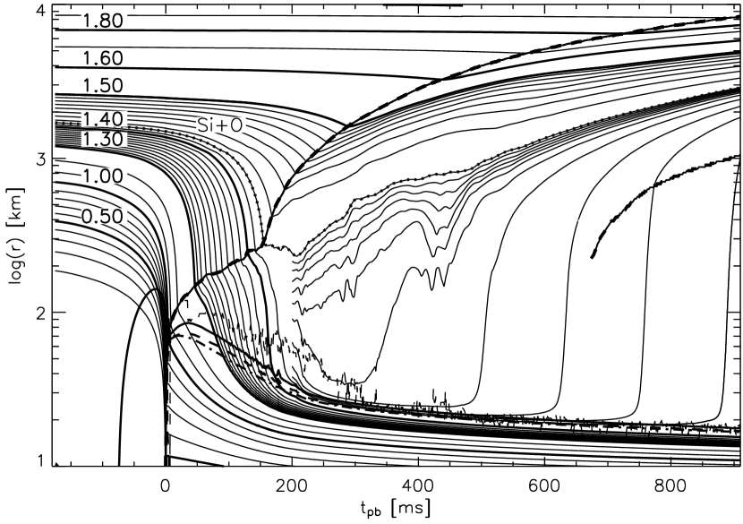
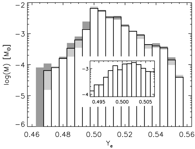
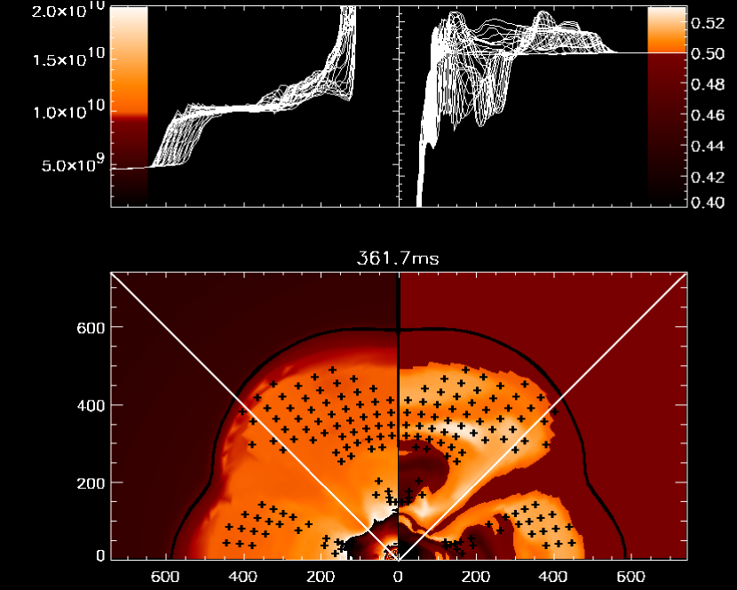
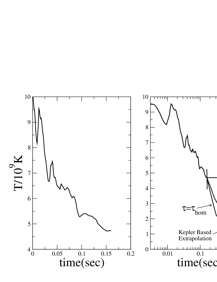
The evolution from the onset of core collapse (at about $-175\,$ms) through core bounce and convective phase to explosion is shown in terms of mass shell trajectories in Fig. 1. The explosion sets in when the infalling interface between Si layer and oxygen-enriched Si layer reaches the shock at about 160 ms post bounce. The corresponding steep drop of the density and mass accretion rate, associated with an entropy increase by a factor of $\sim\,$2, allow the shock to expand and convection to become more violent, thus establishing runaway conditions. The calculation was performed in 2D for following the ejection of the convective shell until 470 ms after bounce. While matter is channeled in narrow downflows towards the gain radius, where it is heated by neutrinos and some of it starts expanding again in high-entropy bubbles, its neutron-to-proton ratio is set by weak interactions with electron neutrinos and antineutrinos as well as electron and positron captures on free nucleons. The final value of ${Y_{\mathrm{e}}}$ is a crucial parameter for the subsequent nucleosynthesis. The mass distribution of neutrino-heated and -processed ejecta from the convective bubble is plotted in Fig. 2.

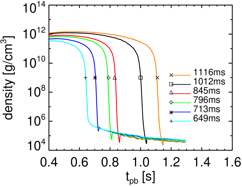
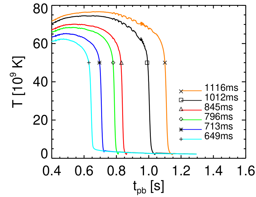
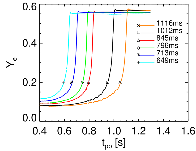
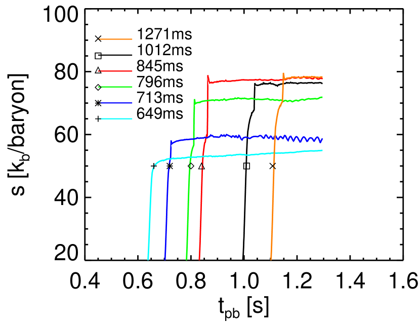
At 470 ms after bounce the model was mapped to a 1D grid and the subsequent evolution was simulated until 1300 ms after bounce. With accretion flows to the neutron star having ceased, this phase is characterized by an essentially spherically symmetric outflow of matter from the nascent neutron star, which is driven by neutrino-energy deposition outside the neutrinosphere (Woosley & Baron, 1992; Duncan, Shapiro, & Wasserman, 1986). This neutrino-powered wind is visible in Fig. 1 after $\sim$500 ms. The fast wind collides with the dense shell of slower ejecta behind the shock and is decelerated again. The corresponding negative velocity gradient steepens to a reverse shock when the wind expansion becomes supersonic (Fig. 1; Janka & Müller 1995). Characteristic parameters for some mass shells in this early wind phase are shown in Fig. 3. Six representative shells are sufficient, because the differences between the shells evolve slowly with time according to the slow variation of the conditions (neutron star radius, gravitational potential, neutrino luminosities and spectra) in the driving region of the wind near the neutron star surface. In Table 3 the masses associated with the different shells are listed.

At the end of the simulated evolution the model has accumulated an explosion energy of approximately $0.6\times 10^{51}\,$erg. The mass cut and thus initial baryonic mass of the neutron star is 1.41 M_⊙. The model fulfills fundamental constraints for Type II SN nucleosynthesis (Hoffman et al., 1996) because the ejected mass having ${Y_{\mathrm{e}}}\lesssim 0.47$ is $\lesssim$10${}^{-4}\,$M_⊙ (see Fig. 2) and thus the overproduction of N=50 (closed neutron shell) nuclei of previous explosion models does not occur. More than 83% of the ejected mass in the convective bubble and early wind phase (in total 0.03 M_⊙ in this rather low-energetic explosion) have ${Y_{\mathrm{e}}}>0.5$. The ejection of mostly p-rich matter is in agreement with 1D general relativistic SN simulations with Boltzmann neutrino transport in which the explosion was launched by artificially enhancing the neutrino energy deposition in the gain layer (Thielemann et al., 2003; Fröhlich et al., 2004). The reason for the proton excess is the capture of electron neutrinos and positrons on neutrons, which is favored relative to the inverse reactions because of the mass difference between neutrons and protons and because electron degeneracy becomes negligible in the neutrino-heated ejecta (Fröhlich et al., 2004; Qian & Woosley, 1996).

Although the explosion in the considered SN model of Janka, Buras, & Rampp (2003) was obtained by a regression from the most accurate treatment of the neutrino transport, it not only demonstrates the proximity of such accurate models to explosions, but also provides a consistent description of the onset of the SN explosion due to the convectively supported neutrino-heating mechanism, and of the early SN evolution. The properties of the resulting explosion are very interesting, including the conditions for nucleosynthesis. The ${Y_{\mathrm{e}}}$ values of the ejecta should be rather insensitive to the manipulation which enabled the explosion. On the one hand the expansion velocities of the high-entropy ejecta are still fairly low (less than a few $10^{8}\,$cm s^-1) when weak interactions freeze out, and on the other hand the omitted velocity-dependent effects affect neutrinos and antineutrinos in the same way.

2.2 Outflows in the Convective Bubble

In order to calculate the nucleosynthesis it is necessary to have a starting composition and the temperature-density ($T-\rho$) history of the matter as it expands and is ejected from the supernova. Because the matter is initially in nuclear statistical equilibrium, the initial values of ${Y_{\mathrm{e}}}$, $T$, and $\rho$ determine the composition which is just protons with a mass fraction ${Y_{\mathrm{e}}}$ and neutrons. We are most interested in the innermost few hundredths to one tenth of a solar mass to be ejected. This matter has an interesting history. It was initially part of the silicon shell of the star, but fell in when the core collapsed, passed through the SN shock and was photodisintegrated to nucleons. Neutrino heating then raised the entropy and energy of the matter causing it to convect. Eventually some portion of this matter gained enough energy to expand and escape from the neutron star, pushing ahead of it the rest of the star. As it cooled, the nucleons reassembled first into helium and then into heavy elements.

The temperature-density history of such matter is thus not given by the simple ansatz often employed in explosive nucleosynthesis — “adiabatic expansion on a hydrodynamic time scale”. In fact, owing to convection, the temperature history may not even be monotonic. Here we rely on tracer particles embedded in the so called “hot convective bubble” of the 15 ${\mathrm{M}_{\odot}}$ SN model calculated by Janka, Buras, & Rampp (2003) (Fig. 4). These tracer particles were not distributed uniformly in mass, but chosen to represent a range of ${Y_{\mathrm{e}}}$ in the ejecta.

The proton-rich outflows of interest here begin at about 190 ms after core bounce (Fig. 1). Entropies and electron fractions characteristic of a few different trajectories are given in Table 2. Each trajectory represents a different mass element in the convective bubble. As is seen, ${Y_{\mathrm{e}}}$ for the different trajectories lies in the range from $0.5-0.546$, and the entropies per nucleon are modest, $s/k_{b}\sim 30-50$. Figure 2 shows the ejected mass versus ${Y_{\mathrm{e}}}$ during the convective phase of the SN explosion.

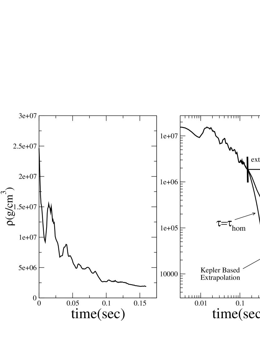
At the end of the 2D calculation of Janka, Buras, & Rampp (2003), the mass element in a typical trajectory had reached a radius of about $2000$ $\mathrm{km}$ (corresponding to the time when the SN model was mapped from 2D to 1D and thus detailed information for the mass elements was lost). Temperatures at this radius were typically $T_{9}\equiv T/10^{9}\,{\rm K}\approx 4$–5, which is still hot enough that nuclei have not yet completely re-assembled. To follow the nucleosynthesis until all nuclear reactions had frozen out it was necessary to extrapolate the trajectories to low temperature. In doing so, we assumed that the electron fraction and entropy were constant during the extrapolated portion of the trajectory. This should be valid because the number of neutrino captures suffered by nuclei beyond $\sim 2000$ $\mathrm{km}$ is small.

We considered two approximations to the expansion which should bracket the actual behavior. The first assumes homologous expansion at a velocity given by the Janka et al. calculation between 10 billion and 4 billion K. This ignores any deceleration experienced as the hot bubble encounters the overlying star and is surely an underestimate of the actual cooling time (though perhaps realistic for the accretion-induced collapse of a bare white dwarf). In particular, we estimated the homologous expansion time scale for each trajectory as $\tau_{\rm hom}=(t_{\mathrm{f}}-t_{\mathrm{i}})/\ln(\rho_{\mathrm{i}}/\rho_{\mathrm{f}})$ where the subscript $\mathrm{i}$ denotes the value of a quantity when $T_{9}=10$ and the subscript $\mathrm{f}$ denotes the value of a quantity at the last time given for the tracer particle history ($t_{\mathrm{f}}\approx 436\,{\rm ms},\,T_{9,{\mathrm{f}}}\approx 4$–5). Values of $\tau_{\rm hom}$ for different trajectories are given in Table 2.

The second approximation was an attempt to realistically represent material catching up with the supernova shock. This extrapolation is based on smoothly merging the trajectories found in the calculations of Janka et al. with those calculated for the inner zone of the same 15 ${\mathrm{M}_{\odot}}$ supernova by Woosley & Weaver (1995). There are some differences. The earlier study was in one dimension and the shock was launched artificially using a piston. The kinetic energy at infinity of the Woosley-Weaver model was $1.2\times 10^{51}$ erg; that of the Janka et al. model was $0.6\times 10^{51}$ erg. Still the calculations agreed roughly in the temperature and density at the time when the evaluation of tracer particles in the current 2D simulation was stopped. In order not to have discontinuities in the entropy at the time when the two calculations are matched, the density in the previous 1D calculation is changed slightly. This merging of the late time trajectories is expected to be reasonable because the shock evolution at several seconds post core bounce is determined mostly by the explosion energy.

We shall see in Sect. 3 that abundances of key nuclei are particularly sensitive to the time it takes the flow to cool from $2\cdot 10^{9}\,$K to $1\cdot 10^{9}\,$K. The homologous expansion approximation gives this time as about 100–200 ms, while the Kepler based estimate gives this time as about 1 sec. Both estimates are rough and should be viewed as representing upper and lowed bounds to the time scale.

Figure 5 shows the evolution of density in a representative trajectory for each of the two approximations to the flow at large radii. The temperature history in these trajectories is shown in Fig. 6. Note the irregular and non-monotonic evolution of the thermodynamic quantities at early times.

2.3 Outflows in the Early Wind

While the shock sweeps through and expels the stellar mantle, matter is still being continuously ablated from the surface of the cooling neutron star. Neutrino heating, principally via charged current neutrino capture, acts to maintain pressure-driven outflow in the tenuous atmosphere formed by the ablated material. This outflow has a higher entropy and is less irregular than the convective bubble.

The evolution of material at radii smaller than a few hundred km is set by characteristics of the cooling neutron star. It is at these small radii that the asymptotic entropy $s$ and electron fraction ${Y_{\mathrm{e}}}$ are set. At early times the neutron star has yet to radiate away the bulk of its gravitational energy and so has a relatively large radius. Material escaping the star during this period only needs to gain a little energy through heating to escape the still shallow gravitational potential. Consequently, the entropy of the asymptotic outflow is about a factor of two smaller than the entropy of winds leaving the neutron star $\sim$10 seconds post core-bounce. This can be seen from the analytic estimate provided by Qian & Woosley (1996)

$$s\approx 235(L_{{\bar{\nu}}_{e},51}\epsilon_{{\bar{\nu}}_{e},{\rm MeV}}^{2})^{-1/6}\left(\frac{10^{6}\,{\mathrm{cm}}}{R}\right)^{2/3}.$$ (1)

Here $L_{{\bar{\nu}}_{e},51}=L_{\bar{\nu}_{e}}/10^{51}{\rm erg/sec}$ , $\epsilon_{{\bar{\nu}}_{e},{\rm MeV}}$ approximately the mean energy of electron anti-neutrinos and $R$ is the neutron star radius. A lower entropy implies a higher density and therefore faster particle capture rates at a given temperature. For proton-rich outflows this typically results in synthesis of heavier elements.

The electron fraction in the outflow is set by a competition between different lepton capture processes on free nucleons:

$$\nu_{e}+{\rm n} \longleftrightarrow {\rm p}+e^{-}\,,$$ (2)

$$e^{+}+{\rm n} \longleftrightarrow {\rm p}+\bar{\nu}_{e}\,.$$ (3)

Because the neutron star is still deleptonizing at early times, the $\nu_{e}$ and $\bar{\nu}_{e}$ spectra can be quite similar. Also, once heating raises the entropy of material leaving the neutron star, the number densities and spectra of electrons and positrons within the material become similar. Under these circumstances the 1.29 MeV threshold for ${\rm p\rightarrow n}$ results in $\bar{\nu}_{e}/e^{-}$ capture rates which are slower than the inverse $\nu_{e}/e^{+}$ capture rates. Weak processes then drive the outflow proton rich. The electron fraction in the wind is mostly set by the competition between $\nu_{e}$ and $\bar{\nu}_{e}$ capture (because $e^{\pm}$ captures freeze out when the density and temperature in the outflow become low, whereas high-energy neutrinos streaming out from the neutrinosphere still continue to react with nucleons). When the composition comes to equilibrium with the neutrino fluxes,

$${Y_{\mathrm{e}}}\,\approx\,\frac{\lambda_{\nu_{e}n}}{\lambda_{\nu_{e}n}+\lambda_{\bar{\nu}_{e}p}}\ .$$ (4)

Here $\lambda_{\nu}$ represents the electron neutrino or antineutrino capture rate on neutrons or protons. Because the star is still deleptonizing at early times, the $\nu_{e}$ and $\bar{\nu}_{e}$ spectra can be quite similar. The 1.29 MeV threshold for $\bar{\nu}_{e}$ capture then leads to $\lambda_{\nu_{e}n}>\lambda_{\bar{\nu}_{e}p}$, and proton-richness is established in the outflow. Finally also the neutrino reactions cease because of the $1/r^{2}$ dilution of the neutrino density with growing distance $r$ from the neutron star.

Table 3 gives characteristics of the early wind found in the simulations of Janka, Buras, & Rampp (2003). As expected, the wind is proton rich at early times. Eventually, the hardening of the $\bar{\nu}_{e}$ spectrum relative to the $\nu_{e}$ spectrum will cause ${Y_{\mathrm{e}}}$ to fall below 1/2. This turnover has not yet occurred when the hydrodynamic simulation was stopped. It should take place at a later time when the wind properties (mass loss rate, entropy) have changed such that the nucleosynthesis constraints for the amount of ${Y_{\mathrm{e}}}<0.47$ ejecta (Hoffman et al., 1996) will not be violated. At 1.3 s after bounce the mass loss rate of about $3\times 10^{-3}\,$M${}_{\odot}\,$s^-1 and wind entropy of $\sim\,$80$\,k_{b}$ per nucleon in the Janka et al. model are likely to still cause an overproduction of N=50 nuclei if ${Y_{\mathrm{e}}}$ went significantly below 0.5.

The temperature in the wind at the end of the traced shell expansion is $T_{9}\approx 2$ (Fig. 3). Approximations for the wind evolution at lower temperatures are the same as those discussed above.

2.4 Nuclear Physics Employed

The reaction network used for the present calculations is given in Table 1. Estimates of reaction rates and nuclear properties used in our calculations are the same as those used in the study of X-ray bursts by Woosley et al. (2004). Briefly, reaction rates were taken from experiment whenever possible, from detailed shell-model based calculations (Fisker et al., 2001) for a few key $({\rm p,\gamma})$ rates, and from Hauser-Feshbach calculations (Rauscher & Thielemann, 2000) otherwise. Proton separation energies, which are crucial determinants of nucleosynthesis in flows with ${{Y_{\mathrm{e}}}>1/2}$, were taken from a combination of experiment (Audi & Wapstra, 1995), the Hartree-Fock Coulomb displacement calculations of Brown et al. (2002) for many important nuclei with Z$>$N, and theoretical estimates (Möller et al., 1995). Choosing the best nuclear binding energies is somewhat involved and we refer the reader to the discussion in Brown et al. (2002) and Fig. 1 of Woosley et al. (2004). Ground-state weak lifetimes are experimentally well determined for the nuclei important in this paper. At temperatures larger than $10^{9}$ K the influence of thermal effects on weak decays was estimated from the compilation of Fuller, Fowler, & Newman (1982) where available. Table 7 gives the nuclei for which the Fuller et al. rates were used. A test calculation in which we switched thermal rates off and used only experimentally determined ground-state rates showed little effect on the important abundances. Section 3.1 contains a discussion of the influence of nuclear uncertainties on yields of some interesting nuclei.

3 Nucleosynthesis Results

Table 2 gives the major calculated production factors for a number of trajectories in the convective bubble and for our two different estimates of the material expansion rate at low temperatures. Table 3 gives production factors for nuclei synthesized in different mass elements comprising the early wind. Here the production factor for nuclide $i$ is defined as

$$P_{i}={M\over M^{\mathrm{ej}}}{X_{i}\over X_{\odot,i}},$$ (5)

where $M$ is the total mass in a given trajectory, $M^{\mathrm{ej}}=13.5\,{\mathrm{M}_{\odot}}$ is the total mass ejected in the SN explosion, $X_{i}$ is the mass fraction of nuclide $i$ in the trajectory, and $X_{\odot,i}$ is the mass fraction of nuclide $i$ in the sun. To aid in interpreting the tables we show in Fig. 7 plots of $X_{i}/X_{\odot,i}$ characterizing the nucleosynthesis in two representative hot-bubble trajectories.

Production factors integrated over the different bubble trajectories are given in Table 4. If one assumes rapid expansion, production factors of ⁴⁵Sc, ⁶³Cu, ⁴⁹Ti, and ⁵⁹Co are all above 1.5. For the slower expansion time scale below $4\times 10^{9}$ K, which we regard as more realistic, a different set of nuclei are produced, especially ⁴⁹Ti and ⁶⁴Zn. Depending upon mass and metallicity, ⁴⁹Ti may already be well produced in other regions of the same supernova (Woosley & Weaver, 1995; Rauscher, Heger, Hoffman, & Woosley, 2002), but ⁶⁴Zn is not. The synthesis here thus represents a new way of making ⁶⁴Zn and this same process will function as well in zero and low metallicity stars as in supernovae today. However, ⁶⁴Zn was already known to be produced, probably in greater quantities, by the neutrino-powered wind (Hoffman et al., 1996).

Production factors integrated over the different wind trajectories are given in Table 5. The somewhat high-entropy wind synthesizes ⁴⁵Sc, ⁴⁹Ti and ⁴⁶Ti more efficiently than the bubble. Typical values of $X/X_{\sun}$ for these three nuclei are approximately $10^{4}$ in the wind and approximately $2\cdot 10^{3}$ in the bubble. In the present calculations the integrated production factor for Sc in the wind is between about 1.5 and 4.7 depending on the time scale describing the wind expansion at $T_{9}\lesssim 2$.

For comparison, in the 15 ${\mathrm{M}_{\odot}}$ supernova of Rauscher, Heger, Hoffman, & Woosley (2002), this production factor was about 7 for many major species, including oxygen. This is close to the combined wind/bubble production factors of Sc and ^46,49Ti in the present calculations. The other most abundant productions in Tables 4 and 5 fall short of this - but not by much. The bulk production factors in a 25 ${\mathrm{M}_{\odot}}$ supernova are about twice those in a 15, but our explosion model is not easily extrapolable to stars of other masses. If 25 ${\mathrm{M}_{\odot}}$ stars explode with a similar kinetic energy it will probably take a more powerful central engine to overcome their greater binding energy and accretion rate during the explosion. Probably this requires more mass in the convective bubble. In fact, the energy of the 15 ${\mathrm{M}_{\odot}}$ supernova used here, $0.6\times 10^{51}$ erg, would be regarded by many as low. It may be that the mass here should be doubled too.

It is important to note that the species listed in Tables 4 and 5 are not made as themselves but as proton-rich radioactive progenitors. Major progenitors of important product nuclei are given in the far right column of Table 4. Typical progenitors of important nuclei are 3–4 charge units from stability. This can be understood through consideration of the Saha equation. Before charged particle reactions freeze out at $T_{9}\approx 1.5-2$, nuclear abundances along an isotonic chain are well approximated as being in local statistical equilibrium:

$$\frac{X({\rm Z+1,N})}{X({\rm Z,N})}\approx 10^{-5}\exp(S_{p}/T)\frac{\rho_{5}}{T_{9}^{3/2}}\frac{G_{\rm Z+1,N}}{G_{\rm Z,N}}.$$ (6)

Here $S_{p}$ is the proton separation energy of the Z+1,N nuclide, $G$ represents the partition function, $\rho_{5}=\rho/10^{5}{{{\mathrm{g}}\,{\mathrm{cm}}^{-3}}}$, $T_{9}=T/10^{9}{\rm K}$, and A=Z+N. Equation (6) predicts that the abundances of nuclei with $S_{p}\lesssim 500$ keV are very small.

Perhaps the most notable feature of the proton-rich trajectories is their inefficiency at synthesizing elements with A$\,\gtrsim\,$60. Neutron-rich outflows, by contrast, readily synthesize nuclides with mass A$\,\sim\,$100. This is shown in Table 6 which gives production factors characterizing nucleosynthesis in somewhat neutron-rich winds occurring in the SN. The Kepler-based extrapolation of the first trajectory in Table 2 is used for these ${Y_{\mathrm{e}}}<0.5$ calculations. Estimates of the mass in each ${Y_{\mathrm{e}}}$ bin for the calculations of Janka, Buras, & Rampp (2003) are shown in Fig. 2.

Termination of the nuclear flow at low mass number in proton-rich outflows has a simple explanation. Unlike nuclei at the neutron drip lines, proton-rich waiting point nuclei have lifetimes much longer than the time scales characterizing expansion of neutrino-driven outflows. In addition, proton capture from waiting point nuclei to more rapidly decaying nuclei is inefficient. To illustrate the difficulty with rapidly assembling heavier proton-rich nuclei, consider nuclear flow through ${}^{64}{\rm Ge}$. This waiting point nucleus has a lifetime of approximately 64 sec. The ratio of the amount of flow leaving ${}^{65}{\rm As}$ to that leaving ${}^{64}{\rm Ge}$ is found from application of the Saha equation above,

$$\frac{\lambda_{+}(^{65}{\rm As})Y(^{65}{\rm As})}{\lambda_{+}(^{64}{\rm Ge})Y(^{64}{\rm Ge})}\approx 10^{-2}\frac{\rho_{5}}{T_{9}^{3/2}}\exp(S_{p}/T).$$ (7)

Here $\lambda_{+}$ represents the $\beta^{+}$ decay rate and $S_{p}$ is the proton separation energy of As. For ${}^{65}{\rm As}$, $\lambda_{+}\approx\ln(2)/0.1\sec$ and for ${}^{64}{\rm Ge}$, $\lambda_{+}\approx\ln(2)/64\sec$. By definition, proton capture daughters of waiting point nuclei are characterized by small proton separation energies. The binding energy of ${}^{65}{\rm As}$ still has large uncertainties, though is known to be less than about 200keV (Brown et al., 2002). Positron decay out of the proton capture daughter of the waiting point nuclei is negligible for such small proton separation energies. These considerations do not hold for X-ray bursts, where time scales characterizing nuclear burning can be tens or hundreds of seconds.

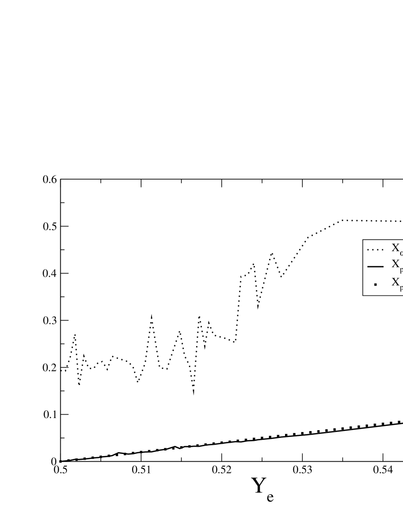
The difficulty with rapid assembly of heavy proton-rich nuclei is also evident in the final free proton and alpha particle mass fractions. The trend of $X_{p}$ and $X_{\alpha}$ with ${Y_{\mathrm{e}}}$ is shown in Fig. 8 for the different Kepler extrapolated bubble trajectories. Also shown in this figure is the proton mass fraction calculated under the assumption that all available nucleons are bound into alpha particles. This is an approximate measure of the mass fraction of available protons. Note that the mass fraction of protons in the two calculations are nearly identical. This is because assembly of proton-rich nuclei occurs on a very slow time scale set by a few $\beta^{+}$ rates.

Because nucleosynthesis past A$\,\sim\,$60 is inefficient these proton-rich flows do not produce N=50 closed shell nuclei. Historically, overproduction of N=50 nuclei has plagued calculations of supernova nucleosynthesis (Howard et al., 1993; Witti et al., 1993; Woosley et al., 1994). The influence of weak interactions in driving some of the outflow to ${{Y_{\mathrm{e}}}>1/2}$ ameliorates this problem.

3.1 Details of the Nucleosynthesis and Critical Nuclear Physics

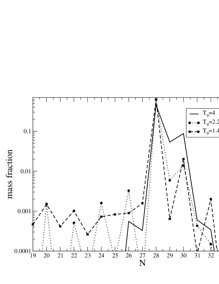
To aid in understanding the general character of these proton-rich flows we show in Fig. 9 the evolution of nuclear mass fractions as a function of the neutron number. At $T_{9}\approx 4$, $\alpha$ captures have led to efficient synthesis of tightly bound species with N=28 and N=30. As temperature decreases $\alpha$ capture becomes less efficient and $\beta^{+}$ decay drives flow to higher neutron number. From Table 4 it is seen that the nuclei we are most interested in arise from decay of nuclei with N=21, 24, 31 and 32. From Fig. 9 it is clear that synthesis of nuclei with these neutron numbers represents a minor perturbation on the nucleosynthesis as a whole.

Tables 4 and 5 show that ${}^{45}{\rm Sc}$, the only stable scandium isotope, has a combined wind/bubble production factor of about 6 if freeze-out is rapid and a combined production factor about 50$\%$ smaller in the slower Kepler extrapolated trajectories. Efficient synthesis of scandium in proton rich outflows associated with Gamma Ray Bursts has been noted previously by Pruet et al. (2004), while Maeda & Nomoto (2003) found that scandium may also be synthesized explosively in shocks exploding anomalously energetic supernovae. Indeed, values presented here for ${{Y_{\mathrm{e}}}}$, $s/k_{b}$, and $\tau$ in the early SN wind are very close to estimates of these quantities in winds leaving the inner regions of accretion disks powering collapsars (MacFadyen & Woosley, 1999; Pruet et al., 2004). The origin of Sc is currently uncertain and it may be quite abundant in low metallicity stars (Cayrel et al., 2004) suggesting a primary origin. In the present calculations the yields of this element are close to those needed to explain the current inventory of Sc.

To understand how synthesis of scandium depends on the outflow parameters and nuclear physics, note that Sc arises mostly from $\beta^{+}$ decay originating with the quasi waiting-point nucleus ${}^{45}{\rm Cr}$. In turn, N=21 isotones of ${}^{45}{\rm Cr}$ originate from $\beta^{+}$ decay out of isotones of ${}^{40}{\rm Ca}$. The doubly magic nucleus ${}^{40}{\rm Ca}$ is efficiently synthesized through a sequence of alpha captures. At temperatures larger than about $2\cdot 10^{9}$ K statistical equilibrium keeps almost all N=20 nuclei locked into ${}^{40}{\rm Ca}$. This nucleus is $\beta$ stable and has a first excited state at 3.3 MeV, too high to be thermally populated. Flow out of N=20 can only proceed when the temperature drops to approximately 1.5 billion degrees and statistical equilibrium favors population of ${}^{42}{\rm Ti}$ over ${}^{40}{\rm Ca}$. The proton capture daughter of ${}^{40}{\rm Ca}$ (${}^{41}{\rm Sc}$) has a proton separation energy of only 1.7 MeV and is not appreciably abundant. Decay out of ${}^{42}{\rm Ti}$ is then responsible for allowing flow to N=21. ${}^{42}{\rm Ti}$ has a well determined $\beta^{+}$ half life of 199$\pm$6 ms, a proton separation energy which is uncertain only by about 5 keV, and a first excited state too high in excitation energy to play a role in allowing flow to N=21. In short, nuclear properties are well determined for important N=20 nuclei. Once nuclei make their way to N=21 at $T_{9}\approx 1.5$, their abundances are divided between the tightly bound ${}^{45}{\rm Cr}$ and ${}^{43}{\rm Ti}$. Here uncertainties in nuclear physics may be more important. For ${}^{45}{\rm Cr}$ the proton separation energy is uncertain to about 100 keV and the spin of the ground state is uncertain. To the extent that the relative abundances are set by the Saha equation, these uncertainties could imply an uncertainty of a factor of several in the relative abundances of ${}^{45}{\rm Cr}$ and ${}^{45}{\rm Ti}$ at $T_{9}\approx 1.5$. In turn, this implies appreciable uncertainty in the estimated Sc yield.

Whether or not Sc is efficiently synthesized following decay of ⁴⁵Cr depends on the expansion time scale at low temperatures. This is because the $\beta^{+}$ daughter of ⁴⁵Cr is ⁴⁵V, which has a relatively small proton separation energy of 1.6 MeV. At low temperatures the Saha equation favors proton capture to ⁴⁶Cr. If the expansion is slow enough that most ⁴⁵Cr decays at temperatures where ${}^{45}{\rm V(p,\gamma)^{46}Cr}$ is still rapid, then flow out of the N=22 nuclei occurs via $\beta^{+}$ decay out of ⁴⁶Cr. In this case ⁴⁶Ti is synthesized rather than ⁴⁵Sc.

${}^{49}{\rm Ti}$ originates from the the N=24 nuclide ${}^{49}{\rm Mn}$. At $T_{9}\approx 1.4$ nuclei with N=24 are divided roughly equally between ${}^{49}{\rm Mn}$ and ${}^{50}{\rm Fe}$. Uncertainties in the proton separation energies and lifetimes of these nuclei are small. ${}^{49}{\rm Mn}$ does have a low lying excited state at 382 keV which is thermally populated at low temperatures. However, ${}^{49}{\rm Mn}$ is a nucleus with Z=N+1 that is expected to have ground and excited state decay rates that are dominated by super-allowed Fermi transitions which are almost independent of excitation energy.

Lastly, we turn our attention to flow out of the N=32 isotones which are progenitors of ${}^{60}{\rm Zn}$ and ${}^{63}{\rm Cu}$. Proton-rich nucleosynthesis near ${}^{64}{\rm Ge}$ has been extensively discussed in the X-Ray Burst literature (e.g. Brown et al. 2002). Uncertainties in basic nuclear properties important for synthesis of ${}^{60}{\rm Zn}$ are small. This is not true for ${}^{63}{\rm Cu}$, which is formed directly by the decay of ${}^{63}{\rm Ga}$. ${}^{63}{\rm Ga}$ has a $J^{\pi}=(5/2)^{-}$excited state at 75.4 keV which dominates the partition function at $T_{9}\approx 1.5$ since the ground state has $J=3/2$. The weak lifetime of this excited state is experimentally undetermined (as are the weak lifetimes of all short lived excited states) and could easily be a factor of five longer or shorter than the quite long ground state lifetime of $\sim 32$ sec. This translates into an uncertainty of a factor of several in the inferred ${}^{63}{\rm Cu}$ yield.

The influence of possible uncertainties in the time scale, entropy, and electron fraction characterizing the different trajectories can be seen from the results in Table 2. Modest changes in the outflow parameters result in factors of $\sim 2$ changes in yields of the most important isotopes. This is evident by the quite different efficiencies with which the lower entropy bubble and higher entropy wind synthesize ⁴⁵Sc and ⁴⁹Ti.

So far we have not considered the influence of neutrino interactions, except implicitly through the setting of ${Y_{\mathrm{e}}}$. If matter remains close to the neutron star, neutrino capture and neutrino-induced spallation may compete with positron decay, even on a dynamic time scale. However, neutrino capture alone cannot act to accelerate nuclear flow past waiting point nuclei and allow synthesis of the heavier proton-rich elements. The reason is that the neutrino capture rates on the waiting point nuclei are about the same as the rate of neutrino capture on a free proton (Woosley et al., 1990). Every capture of a neutrino by a heavy nucleus is accompanied by a capture onto a free proton. The electron fraction is then rapidly driven to $1/2$ since the neutron produced in this way immediately goes into the formation of an $\alpha$-particle. This is analogous to the “$\alpha$-effect” discussed in the context of late-time winds (Fuller & Meyer, 1995; Meyer et al., 1998).

4 Conclusions and Implications

The important news is that, unlike simulations of a few years ago, there is no poisonous overproduction of neutron-rich nuclei in the vicinity of the N = 50 closed shell (Woosley et al., 1994). When followed in more detail (i.e. mainly with a better, spectral treatment of the neutrino transport), weak interactions in the hot convective bubble drive ${Y_{\mathrm{e}}}$ back to 0.5 and above so that most of the mass comes out as ⁵⁶Ni and ⁴He. Since ⁵⁶Fe and helium are abundant in nature, this poses no problem.

Beyond this it is also interesting that the proton-rich environment of the hot convective bubble and early neutrino-driven wind can synthesize interesting amounts of some comparatively rare intermediate mass elements. If the total mass of SN ejecta with ${Y_{\mathrm{e}}}\gtrsim 0.5$ is larger than a few hundredths of a solar mass, these proton-rich outflows may be responsible for a significant fraction of the solar abundances of ${}^{45}{\rm Sc}$, ${}^{64}{\rm Zn}$, and some Ti isotopes, especially ⁴⁹Ti.

However, these ejecta do not appear to be implicated in the synthesis of elements that do not have other known astrophysical production sites. For example, ${\rm Sc}$ can be produced explosively, while ${}^{64}{\rm Zn}$ can be synthesized in a slightly neutron-rich wind. It seems unlikely that consideration of nucleosynthesis in proton-rich outflows will lead to meaningful constraints on conditions during the early SN.

Since the conditions in the hot convective bubble resemble in some ways those of Type I X-ray bursts (high temperature and proton mass fraction), we initially hoped that the nuclear flows would go higher, perhaps producing the $p$-process isotopes of Mo and Ru. Such species have proven difficult to produce elsewhere and the $rp$-process in X-ray bursts can go up as high as tellurium (Schatz et al., 2001). Unfortunately the density is much less here than in the neutron star and the time scale shorter. Proton-induced flows are weaker and the leakage through critical waiting point nuclei is smaller. Using the present nuclear physics, significant production above A = 64 is unlikely. However, heavier nuclei can be produced in ejecta that are right next to these zones but with values of ${Y_{\mathrm{e}}}$ considerably less than 0.50 (Hoffman et al., 1996).

Table 1: Reaction Network Used for the Present Calculations

Element	${\rm N_{\rm min}}$	${\rm N_{\rm max}}$	Element	${\rm N_{\rm min}}$	${\rm N_{\rm max}}$	Element	${\rm N_{\rm min}}$	${\rm N_{\rm max}}$
H	1	2	He	1	4	Li	3	6
Be	3	8	B	3	9	C	3	12
N	4	14	O	5	14	F	5	17
Ne	6	21	Na	6	33	Mg	6	35
Al	7	38	Si	8	40	P	8	42
S	8	44	Cl	8	46	Ar	9	49
K	11	51	Ca	10	53	Sc	13	55
Ti	12	58	V	15	60	Cr	14	62
Mn	17	64	Fe	16	66	Co	19	69
Ni	18	71	Cu	21	73	Zn	21	75
Ga	24	77	Ge	23	80	As	26	82
Se	25	84	Br	28	86	Kr	27	88
Rb	31	91	Sr	30	93	Y	33	95
Zr	32	97	Nb	35	99	Mo	35	102
Tc	38	104	Ru	37	106	Rh	40	108
Pd	40	110	Ag	41	113	Cd	42	115
In	43	117	Sn	44	119	Sb	46	120
Te	47	121

Table 2: Characteristics of nucleosynthesis in some representative bubble trajectories

Trajectory	${Y_{\mathrm{e}}}$	$s/k_{b}$	${\tau_{\rm hom}}$ (sec)	$m/{\mathrm{M}_{\odot}}$	Production ($\tau_{\rm dyn}={\tau_{\rm hom}}$)	Production (Kepler Based Extrapolation)
1	0.500	18.4	0.086	9.25e-04	${}^{59}{\rm Co}$(0.33)	${}^{64}{\rm Zn}$(0.17)
					${}^{64}{\rm Zn}$(0.12)	${}^{59}{\rm Co}$(0.17)
					${}^{49}{\rm Ti}$(0.10)	${}^{49}{\rm Ti}$(0.16)
5	0.502	15.9	0.066	7.05e-04	${}^{59}{\rm Co}$(0.17)	${}^{64}{\rm Zn}$(0.30)
					${}^{63}{\rm Cu}$(0.15)	${}^{49}{\rm Ti}$(0.14)
					${}^{49}{\rm Ti}$(0.12)	${}^{60}{\rm Ni}$(0.09)
10	0.505	21.7	0.062	3.58e-04	${}^{59}{\rm Co}$(0.07)	${}^{64}{\rm Zn}$(0.10)
					${}^{63}{\rm Cu}$(0.05)	${}^{49}{\rm Ti}$(0.09)
					${}^{49}{\rm Ti}$(0.05)	${}^{46}{\rm Ti}$(0.04)
20	0.513	17.8	0.104	4.63e-04	${}^{45}{\rm Sc}$(0.14)	${}^{49}{\rm Ti}$(0.19)
					${}^{46}{\rm Ti}$(0.06)	${}^{64}{\rm Zn}$(0.07)
					${}^{42}{\rm Ca}$(0.05)	${}^{60}{\rm Ni}$(0.05)
30	0.521	26.2	0.047	2.67e-04	${}^{59}{\rm Co}$(0.03)	${}^{49}{\rm Ti}$(0.08)
					${}^{45}{\rm Sc}$(0.02)	${}^{64}{\rm Zn}$(0.03)
					${}^{63}{\rm Cu}$(0.02)	${}^{60}{\rm Ni}$(0.02)
35	0.524	26.9	0.062	2.28e-04	${}^{45}{\rm Sc}$(0.07)	${}^{49}{\rm Ti}$(0.13)
					${}^{42}{\rm Ca}$(0.04)	${}^{46}{\rm Ti}$(0.03)
					${}^{46}{\rm Ti}$(0.03)	${}^{64}{\rm Zn}$(0.03)
40	0.545	40.6	0.024	3.12e-04	${}^{42}{\rm Ca}$(0.04)	${}^{49}{\rm Ti}$(0.25)
					${}^{45}{\rm Sc}$(0.04)	${}^{46}{\rm Ti}$(0.06)
					${}^{46}{\rm Ti}$(0.03)	${}^{45}{\rm Sc}$(0.04)

Table 3: Production factors in the early wind

${Y_{\mathrm{e}}}$	$s/k_{b}$	${\tau_{\rm hom}}$ (sec)	$m/{\mathrm{M}_{\odot}}$	Production ($\tau_{\rm dyn}={\tau_{\rm hom}}$)	Production (Kepler Based Extrapolation)
0.551	54.8	0.131	1.53e-03	${}^{45}{\rm Sc}$(1.73)	${}^{49}{\rm Ti}$(2.02)
				${}^{49}{\rm Ti}$(0.97)	${}^{46}{\rm Ti}$(0.70)
				${}^{46}{\rm Ti}$(0.87)	${}^{45}{\rm Sc}$(0.36)
0.558	58.0	0.127	6.40e-04	${}^{45}{\rm Sc}$(0.95)	${}^{49}{\rm Ti}$(1.09)
				${}^{49}{\rm Ti}$(0.52)	${}^{46}{\rm Ti}$(0.38)
				${}^{46}{\rm Ti}$(0.48)	${}^{45}{\rm Sc}$(0.20)
0.559	76.7	0.099	6.80e-04	${}^{45}{\rm Sc}$(0.60)	${}^{49}{\rm Ti}$(1.07)
				${}^{49}{\rm Ti}$(0.38)	${}^{46}{\rm Ti}$(0.41)
				${}^{46}{\rm Ti}$(0.31)	${}^{45}{\rm Sc}$(0.22)
0.560	71.0	0.112	4.80e-04	${}^{45}{\rm Sc}$(0.55)	${}^{49}{\rm Ti}$(0.79)
				${}^{49}{\rm Ti}$(0.31)	${}^{46}{\rm Ti}$(0.29)
				${}^{46}{\rm Ti}$(0.27)	${}^{45}{\rm Sc}$(0.15)
0.568	74.9	0.059	8.00e-04	${}^{45}{\rm Sc}$(0.55)	${}^{49}{\rm Ti}$(1.25)
				${}^{46}{\rm Ti}$(0.35)	${}^{46}{\rm Ti}$(0.47)
				${}^{49}{\rm Ti}$(0.35)	${}^{45}{\rm Sc}$(0.25)
0.570	76.9	0.034	1.04e-03	${}^{46}{\rm Ti}$(0.38)	${}^{49}{\rm Ti}$(1.49)
				${}^{45}{\rm Sc}$(0.35)	${}^{46}{\rm Ti}$(0.57)
				${}^{42}{\rm Ca}$(0.31)	${}^{45}{\rm Sc}$(0.31)

Table 4: Production factors integrated over the different bubble trajectories

nucleus	Production ($\tau_{\rm dyn}={\tau_{\rm hom}}$)	Production (Kepler Based Extrapolation)	Major Progenitor(s)
${}^{59}{\rm Co}$	2.81	0.37	${}^{59}{\rm Cu},^{59}{\rm Zn}$
${}^{49}{\rm Ti}$	2.00	6.53	${}^{49}{\rm Mn}$
${}^{63}{\rm Cu}$	1.91	0.28	${}^{63}{\rm Ga},^{63}{\rm Ge}$
${}^{45}{\rm Sc}$	1.65	1.33	${}^{45}{\rm Cr}$
${}^{64}{\rm Zn}$	1.28	3.61	${}^{64}{\rm Ge}$
${}^{46}{\rm Ti}$	1.22	1.97	${}^{46}{\rm Cr}$
${}^{60}{\rm Ni}$	1.10	1.81	${}^{60}{\rm Zn}$
${}^{42}{\rm Ca}$	1.04	0.46	${}^{42}{\rm Ti}$

Table 5: Integrated production factors for the early wind

nucleus	Production ($\tau_{\rm dyn}={\tau_{\rm hom}}$)	Production (Kepler Based Extrapolation)
${}^{45}{\rm Sc}$	4.74	1.50
${}^{49}{\rm Ti}$	2.83	7.70
${}^{46}{\rm Ti}$	2.66	2.81
${}^{42}{\rm Ca}$	2.16	0.46
${}^{51}{\rm V\ }$	1.09	0.90
${}^{50}{\rm Cr}$	0.56	0.09

Table 6: Characteristics of Nucleosynthesis in Neutron Rich Trajectories

${Y_{\mathrm{e}}}$	$m/{\mathrm{M}_{\odot}}$	Production
0.470	6.40e-05	${}^{74}{\rm Se}$(6.59)
		${}^{78}{\rm Kr}$(4.25)
		${}^{64}{\rm Zn}$(1.35)
0.475	7.98e-05	${}^{64}{\rm Zn}$(1.36)
		${}^{74}{\rm Se}$(0.85)
		${}^{78}{\rm Kr}$(0.78)
0.480	1.59e-04	${}^{64}{\rm Zn}$(1.49)
		${}^{78}{\rm Kr}$(0.34)
		${}^{68}{\rm Zn}$(0.30)
0.485	3.36e-04	${}^{62}{\rm Ni}$(0.92)
		${}^{58}{\rm Ni}$(0.35)
		${}^{64}{\rm Zn}$(0.23)
0.490	6.24e-04	${}^{62}{\rm Ni}$(1.21)
		${}^{58}{\rm Ni}$(0.42)
		${}^{66}{\rm Zn}$(0.13)
0.495	1.36e-03	${}^{62}{\rm Ni}$(1.30)
		${}^{58}{\rm Ni}$(0.41)
		${}^{61}{\rm Ni}$(0.23)

Table 7: Nuclei for which thermal weak rates are included

Atomic mass	Elements
21	F, Mg, Na, Ne, O
22	Mg, Na, Ne
23	F, Mg, Na, Ne
24	Mg, Na, Ne, Si
25	Mg, Na, Ne, Si
26	Mg, Na, Si
27	Mg, Na, P, Si
28	Mg, Na, P, S, Si
29	Mg, Na, P, S, Si
30	P, S, Si
31	Cl, P, S, Si
32	Cl, P, S, Si
33	Cl, P, S, Si
34	Cl, P, S, Si
35	Cl, K, P, S
36	Ca, Cl, K, S
37	Ca, Cl, K, S
38	Ca, Cl, K, S
39	Ca, Cl, K
40	Ca, Cl, K, Sc, Ti
41	Ca, Cl, K, Sc, Ti
42	Ca, K, Sc, Ti
43	Ca, Cl, K, Sc, Ti
44	Ca, K, Sc, Ti, V
45	Cr, K, Sc, Ti, V
46	Cr, K, Sc, Ti, V
47	Cr, K, Sc, Ti, V
48	Cr, K, Sc, Ti, V
49	Cr, Fe, K, Mn, Sc, Ti, V
50	Cr, Mn, Sc, Ti, V
51	Mn, Sc, Ti, V
52	Fe, Mn, Ti, V
53	Cr, Fe, Mn, Ti, V
54	Cr, Fe, Mn, V
55	Cr, Fe, Mn, Ti, V
56	Cr, Fe, Mn, Ni, Sc, Ti, V
57	Cr, Cu, Fe, Mn, Ni, Ti, V, Zn
58	Cr, Cu, Fe, Mn, Ni, Ti, V
59	Cr, Cu, Fe, Mn, Ni, V
60	Cr, Cu, Fe, Mn, Ni, Ti, V, Zn

Figure 1: Radius versus post-bounce time for selected “mass shells” in the exploding SN model of Janka, Buras, & Rampp (2003), spaced with intervals between 0.001 M_⊙ and 0.1 M_⊙. The simulation was carried out in two dimensions until about 470 ms after bounce, and was continued in spherical symmetry thereafter. During the 2D period the lines do not trace the trajectories of Lagrangian mass elements but correspond to the radii of spheres enclosing certain values of the integrated rest mass. The expanding dashed lines mark the positions of forward shock and wind termination shock, respectively, and the thin dashed, wiggled line represents the angularly averaged position of the gain radius. The neutrinosphere positions of electron neutrinos (solid), electron antineutrinos (dashed), and muon and tau neutrinos and antineutrinos (dash-dotted) are also indicated. The explosion sets in when the shock passes the infalling interface between the Si layer and the oxygen-enriched Si layer (given by the trajectory marked with dots) at which the density begins to drop steeply and the entropy increases from about 2.5 to nearly 5$\,k_{b}$ per nucleon.

Figure 2: Ejecta mass versus ${Y_{\mathrm{e}}}$ of neutrino-heated and -processed matter during the convective phase until $\sim$470 ms post bounce. The insert shows the region around ${Y_{\mathrm{e}}}\sim 0.5$ in higher resolution. The grey shading indicates estimated errors due to the limited spatial resolution of the two-dimensional simulation (for details, see Buras et al. 2004).

Figure 3: Density, temperature, ${Y_{\mathrm{e}}}$, and entropy as functions of post-bounce time along the trajectories of mass elements around an enclosed baryonic mass of 1.41 M_⊙. The elements first follow the rise of temperature and density in the outer layers of the contracting neutron star and then enter a phase of very rapid expansion when they are ejected in the neutrino-driven wind. The curves are labeled by the time the mass elements cross a radius of 100 km. The collision with the slower preceding ejecta occurs through a wind termination shock and is visible as a non-monotonicity of the density and temperature, associated with an entropy increase of 10–15$\,k_{b}$ per nucleon.

Figure 4: Convective bubble around the central neutron star in the two-dimensional SN model of Janka, Buras, & Rampp (2003). Time in this figure is measured from the onset of collapse, core bounce was at 175 ms, the length scale is in km. The panels on the left show the temperature in Kelvin, those on the right ${Y_{\mathrm{e}}}$. The upper plots give radial profiles for all angular bins of the polar coordinate grid of the simulation, which was carried out in a lateral wedge of $\pm 43.2^{\mathrm{o}}$ (with periodic boundary conditions) around the equatorial plane. The latter is indicated by white diagonal lines. The positions of the tracer particles at the onset of the explosion are marked by crosses in the lower panels. Their positions were chosen (by post-processing the finished simulation) such that the ${Y_{\mathrm{e}}}$ distribution of the final ejecta was appropriately represented.

Figure 5: Illustration of the density evolution for hot-bubble trajectory 10 in the two-dimensional SN model of Janka, Buras, & Rampp (2003) (left panel) and as extrapolated for the present nucleosynthesis calculations (right panel).

Figure 6: Evolution of temperature in the trajectory displayed in Fig. 5.

Figure 7: Overproduction plot for nucleosynthesis in some of the tracer particle trajectories in the convective bubble of the SN model of Janka, Buras, & Rampp (2003). Results for two assumptions about the dynamic time scale are shown for each trajectory.

Figure 8: Final proton and $\alpha$ particle mass fractions as a function of ${Y_{\mathrm{e}}}$ for the different Kepler extrapolated trajectories. The line labeled with $X_{p}({\rm theory})$ is the proton mass fraction calculated under the assumption that all available nucleons are locked into alpha particles or other nuclei with equal and even numbers of protons and neutrons.

Figure 9: Evolution of nuclear abundances as a function of neutron number in the Kepler based extrapolation for the hot-bubble trajectory 26 (${Y_{\mathrm{e}}}=0.5172$).

References

- Audi & Wapstra (1995) Audi, G. & Wapstra, A.H. 1995, Nucl. Phys. A, 595, 409
- Brown et al. (2002) Brown, B.A., Clement, R.R., Schatz, H., Volya, A. & Richter, W.A. 2002, Phys. Rev. C, 65, 5802
- Buras et al. (2003) Buras, R., Rampp, M., Janka, H.-T., & Kifonidis, K. 2003, PRL, 90, 241101
- Buras et al. (2004) Buras, R., Rampp, M., Janka, H.-T., Kifonidis, K., Takahashi, K., & Horowitz, C.J. 2004, in preparation
- Cardall & Fuller (1997) Cardall, C. Y. & Fuller, G. M. 1997, ApJL, 486, 111
- Cayrel et al. (2004) Cayrel, R., et al. 2004, A&A, 416, 1117
- Duncan, Shapiro, & Wasserman (1986) Duncan, R.C., Shapiro, S.L., & Wasserman, I. 1986, ApJ, 309, 141
- Fisker et al. (2001) Fisker, J.L., Barnard, V., Gorres, J., Langanke, K., Mártinez-Pinedo, G. & Wiescher, M.C. 2001, At. Data Nucl. Data Tables, 79, 241
- Fröhlich et al. (2004) Fröhlich, C., et al. 2004, Nucl. Phys. A, submitted (astro-ph/0408067)
- Fuller, Fowler, & Newman (1982) Fuller, G.M., Fowler, W.A., & Newman, M.J. 1982, ApJ, 252, 715
- Fuller & Meyer (1995) Fuller, G.M. & Meyer, B.S. 1995, ApJ, 453, 792
- Hoffman et al. (1996) Hoffman, R. D., Woosley, S. E., Fuller, G. M., & Meyer, B. S. 1996, ApJ, 460, 478
- Hoffman, Woosley, & Qian (1997) Hoffman, R. D., Woosley, S. E., & Qian, Y.-Z. 1997, ApJ, 482, 951
- Howard et al. (1993) Howard, W.M., Goriely, S., Rayet, M., & Arnould, M. 1993, ApJ, 417, 713
- Janka (2001) Janka, H.-T. 2001, A&A, 368, 527
- Janka & Müller (1995) Janka, H.-T. & Müller, E. 1995, ApJ, 448, L109
- Janka, Buras, & Rampp (2003) Janka, H.-T., Buras, R., & Rampp, M. 2003, Nucl. Phys. A, 718, 269
- Janka et al. (2004) Janka, H.-T., Buras, R., Kifonidis, K., Rampp, M., & Plewa, T. 2004, in Stellar Collapse, ed. C.L. Fryer, Kluwer, Dordrecht, p. 65
- MacFadyen & Woosley (1999) MacFadyen, A.I. & Woosley, S.E. 1999, ApJ, 524, 262
- Maeda & Nomoto (2003) Maeda, K. & Nomoto, K. 2003, ApJ, 598, 1163
- Meyer et al. (1998) Meyer, B.S., McLaughlin, G.C., & Fuller, G.M. 1998, Phys. Rev. C, 58, 3696
- Möller et al. (1995) Möller, P., Nix, J.R., Myers, W.D., & Swiatecki, W.J. 1995, At. Data Nucl. Data Tables, 59, 185
- Otsuki et al. (2000) Otsuki, K., Tagoshi, H., Kajino, T., & Wanajo, S.-Y. 2000, ApJ, 533, 424
- Pruet et al. (2004) Pruet, J., Surman, R. & McLaughlin, G.C. 2004, ApJ, 602, L101
- Pruet et al. (2004) Pruet, J., Thompson, T.A., & Hoffman, R.D. 2004, 606, 1006
- Qian & Wasserburg (2000) Qian, Y.-Z. & Wasserburg, G. J. 2000, Phys. Reps., 333, 77
- Qian & Woosley (1996) Qian, Y.-Z. & Woosley, S.E. 1996, ApJ, 471, 331
- Rampp & Janka (2002) Rampp, M. & Janka, H.-T. 2002, A&A, 396, 361
- Rauscher & Thielemann (2000) Rauscher, T. & Thielemann, F.-K. 200, At. Data Nucl. Data Tables, 75, 1
- Rauscher, Heger, Hoffman, & Woosley (2002) Rauscher, T., Heger, A., Hoffman, R. D., & Woosley, S. E. 2002, ApJ, 576, 323
- Schatz et al. (2001) Schatz, H., et al. 2001, Physical Review Letters, 86, 3471
- Sumiyoshi et al. (2000) Sumiyoshi, K., Suzuki, H., Otsuki, K., Teresawa, M., & Yamada, S. 2000, PASJ, 52, 601
- Takahashi, Witti, & Janka (1994) Takahashi, K., Witti, J., & Janka, H.-T. 1994, A&A, 286, 857
- Thielemann et al. (2003) Thielemann, F.-K., et al. 2003, Nucl. Phys. A, 718, 139
- Thompson, Burrows, & Meyer (2001) Thompson, T. A., Burrows, A., & Meyer, B. S. 2001, ApJ, 562, 887
- Wallace & Woosley (1981) Wallace, R. K. & Woosley, S. E. 1981, ApJS, 45, 389
- Witti et al. (1993) Witti, J., Janka, T.-H., & Takahashi, K. 1993, A&A, 286, 841
- Woosley & Baron (1992) Woosley, S.E. & Baron, E. 1992, ApJ, 391, 228
- Woosley, Arnett, & Clayton (1973) Woosley, S.E., Arnett, W.D., & Clayton, D.D. 1973, ApJS, 26, 231
- Woosley et al. (1990) Woosley, S.E., Hartmann, D.H., Hoffman, R.D. & Haxton, W.C. 1990, ApJ, 356, 272
- Woosley & Hoffman (1992) Woosley, S.E. & Hoffman, R.D. 1992, ApJ, 395, 202
- Woosley & Weaver (1995) Woosley, S.E. & Weaver, T.A. 1995, ApJS, 101, 181
- Woosley, Heger, & Weaver (2002) Woosley, S.E., Heger, A., & Weaver, T.A. 2002, Reviews of Modern Physics, 74, 1015
- Woosley et al. (1994) Woosley, S.E., Wilson, J.R., Mathews G.J., Hoffman, R.D., & Meyer, B.S. 1994, ApJ, 433, 209
- Woosley et al. (2004) Woosley, S.E., et al. 2004, ApJS, 151, 75