Baryon Oscillations and Dark-Energy Constraints from Imaging Surveys

Abstract

Baryonic oscillations in the galaxy power spectrum have been studied as a way of probing dark-energy models. While most studies have focused on spectroscopic surveys at high redshift, large multi-color imaging surveys have already been planned for the near future. In view of this, we study the prospects for measuring baryonic oscillations from angular statistics of galaxies binned using photometric redshifts. We use the galaxy bispectrum in addition to the power spectrum; this allows us to measure and marginalize over possibly complex galaxy bias mechanisms to get robust cosmological constraints. In our parameter estimation we allow for a weakly nonlinear biasing scheme that may evolve with redshift by two bias parameters in each of ten redshift bins. We find that a multi-color imaging survey that probes redshifts beyond one can give interesting constraints on dark-energy parameters. In addition, the shape of the primordial power spectrum can be measured to better accuracy than with the CMB alone. We explore the impact of survey depth, area, and calibration errors in the photometric redshifts on dark-energy constraints.

1 Introduction

Recent cosmological observations have provided strong evidence that a dark-energy component, such as the cosmological constant, comprises as much as 70 per cent of the total energy density of the universe (Perlmutter et al. 1999; Riess et al. 1998, 2001; Tonry et al. 2003; Spergel et al. 2003). Characterizing the nature of the dark energy and its possible evolution has become a central goal of empirical work in cosmology.

Galaxy surveys measure the clustering statistics of galaxies as a function of scale and redshift. The galaxy power spectrum can be compared to the CMB power spectrum to constrain the growth of structure. However the amplitude of the galaxy power spectrum depends on the biasing of the particular galaxy sample; one therefore needs to exercise care in using the full power spectrum for cosmological inferences (e.g. Tegmark et al. 2004; Pope et al. 2004). The shape of the power spectrum has been regarded as more robust to biasing effects.

The baryon oscillations in the galaxy power spectrum are imprints from acoustic oscillations in the early universe, prior to recombination. The same physics produces the dramatic peaks and troughs seen in the CMB power spectrum. Their physical scale is set by the sound horizon at recombination, which has been determined accurately from CMB data (Spergel et al. 2003). The baryon oscillations in the matter and galaxy power spectra are much weaker features because the dark matter which dominates the mass density did not participate in the acoustic oscillations. The oscillations are at the level of a few tens of a percent variation about the smoothed power spectrum. With a survey of sufficient size, these features can be measured accurately. Since the physical length scale of the baryon oscillations is known from the CMB measurement of the sound horizon, a measurement of their apparent size in redshift or angle space leads to a measurement of purely geometric quantities: the Hubble parameter and the angular diameter distance, respectively. We will be concerned with the relation between physical size and angular diameter distance: $r_{\mathrm{physical}}=d_{\mathrm{A}}(z)\Delta\theta$, where $d_{\mathrm{A}}$ is the angular diameter distance and $\Delta\theta$ is the measured angular scale. This relation can be used for a statistical quantity as well; for the power spectrum it means that a measurement of an angular wavenumber $l$ and its relation to the physical wavenumber $k$ yields $d_{\mathrm{A}}(z)$. We describe in the next section how $d_{\mathrm{A}}$ constrains models of dark energy.

To measure baryon oscillations, many authors have considered galaxy surveys over different redshift ranges (Eisenstein 2003; Blake & Glazebrook 2003; Linder 2003; Hu & Haiman 2003; Seo & Eisenstein 2003; Matsubara & Szalay 2003). For spectroscopic redshift surveys, the tangential and radial components are considered separately since the latter is subject to redshift distortions. Current redshift surveys can map large enough volumes at redshifts well below 0.5. It is a great advantage to probe higher redshifts since additional baryon oscillations can then be measured within the linear regime of clustering (the linear regime extends to smaller physical scales at high redshifts). With future redshift surveys, such as the proposed KAOS survey, such a measurement would be possible.

Multi-color imaging surveys are already in progress, e.g. the SDSS, the CFH Legacy survey, and deeper surveys are proposed for the future, e.g. PANSTARRS, LSST, SNAP and others. These surveys offer the possibility of photometric redshifts as crude redshift estimators. With the SDSS providing a large sample of relatively nearby galaxies, and the Hubble Deep Fields and the GOODS survey providing deep samples of galaxies beyond $z=1$, many multi-color samples of galaxies have been studied and used to estimate photometric redshifts. With good photometry in 4–5 optical filters, it is expected that a statistical accuracy characterized by an rms of $\sigma_{z}\simeq 0.02-0.04$ in $1+z$ is achievable for galaxies below $z=1$. For special samples such as the Large Red Galaxy (LRG) sample of the SDSS, one can do significantly better. Similarly it is expected that with more filters and experience with estimating photo-$z$’s, the accuracy will improve and extend to higher redshifts. This is an area of ongoing study (e.g. Connolly et al. 2002; Budavari et al. 2003; Mobasher et al. 2004).

The accuracy of photometric redshifts determines the bin width in redshift within which angular power spectra can be measured and regarded as being independent of neighboring bins (i.e. the overlap in the galaxy distribution between neighboring bins is small). This is important because wide bins would cause the baryon wiggle features to be smeared out. Following Seo & Eisenstein (2003) we will assume that $\sigma_{z}<0.04$ in $1+z$. Note that this is not a very stringent requirement; at $z=1$, it means the rms error in the photometric redshift is below $0.08$. Given a large number $N$ of galaxies with photo-$z$’s, the mean redshift is measured accurately since the error in it is suppressed by $\sqrt{N}$, which can be very small even per redshift bin for surveys of several 100 or 1000 square degrees. However, when the photo-$z$’s are estimated in terms of a probability distribution over redshift per galaxy, often the result is bi-modal or worse. Thus there are sometimes large errors in the estimated photo-$z$, and for certain redshift ranges they lead to systematic biases. While calibration with spectroscopic redshifts of some fraction of the galaxies can be used to limit such a bias, we will explore the sensitivity of our dark-energy constraints to possible biases in the mean bin redshift.

Our focus will be on the question: can subtle effects in the biasing of galaxies compromise the dark-energy constraints obtained from them? We will use the bispectrum, the Fourier transform of the three-point function, as an independent measure of the biasing of galaxies. The idea of using the bispectrum in addition to the power spectrum on large scales to constrain both the amplitude of the mass power spectrum and bias has been suggested and implemented (Fry 1999; Frieman & Gaztanaga 1999; Feldman et al. 2001; Verde et al. 2002). In this study we will examine whether it can help constrain a possibly redshift dependent bias that could mimic effects of the cosmological model we are trying to constrain. We will also compute the gain in signal to noise that the bispectrum provides. We will use perturbation theory, valid in the weakly nonlinear regime of clustering.

2 Theory

2.1 Dark-Energy Cosmology

The expansion history of the universe is given by the scale factor $a(t)$ in a homogeneous and isotropic universe. For cosmological purposes, dark energy is associated with a density field, possibly weakly evolving over cosmic time, that affects the expansion rate of the universe, $H(a)$. The expansion rate at late cosmic times depends on contributions from the density of non-relativistic matter, $\Omega_{\mathrm{m}}$ (cold dark matter plus baryons), and the dark-energy density, $\Omega_{\mathrm{de}}$. Our notation is such that $\Omega_{\mathrm{m}}$ and $\Omega_{\mathrm{de}}$ denote the present day values in units of the critical density, $3H_{0}^{2}/(8\pi G)$. The dark-energy formalism introduces a new, time-dependent density described by the dark-energy equation of state:

$$w(a):=\frac{p_{\mathrm{de}}}{\rho_{\mathrm{de}}}=-\frac{1}{3}\frac{\mathrm{d}\ln\rho_{\mathrm{de}}}{\mathrm{d}\ln a}-1.$$ (1)

This density component is allowed to have an arbitrary time dependence; it must be constrained by theory and observation. Due to lack of compelling theoretical models for the dark energy, it is typical to introduce a parameterization for $w(a)$ to be determined empirically. We follow Linder (2003) and parameterize the equation of state as

$$w(a)=w_{0}+w_{a}(1-a).$$ (2)

Note that setting $w=-1$, i.e., $w_{0}=-1$ and $w_{a}=0$, corresponds to the equation of state for a cosmological constant.

We assume a flat universe throughout this paper. The expansion rate for a flat universe with dark energy is given by

$$H^{2}(a)=H_{0}^{2}\left\{\Omega_{\mathrm{m}}a^{-3}+\Omega_{\mathrm{de}}e^{-3\int_{1}^{a}\mathrm{d}\ln a^{\prime}\left[1+w(a^{\prime})\right]}\right\}.$$ (3)

The modification in the expansion rate of the universe by a dynamically evolving dark-energy component, as opposed to a cosmological constant for example, alters distance measurements on cosmological scales. The (comoving) distance, $\chi(a)$, from an observer at redshift zero to a source at scale factor $a=1/(1+z)$ is given by:

$$\chi(a)=\int_{a}^{1}\frac{\mathrm{d}a^{\prime}}{H(a^{\prime})a^{\prime 2}}.$$ (4)

Hence, given a cosmological standard ruler, such as the length scale associated with one of the peaks of baryon-induced oscillations in the power spectrum at a given redshift, one may obtain dark-energy constraints via constraints on the distance function.

Dark energy that has negative pressure, i.e., $\rho_{\mathrm{de}}+3p_{\mathrm{de}}<0$ as observed today, leads to repulsive gravity and therefore does not cluster significantly. True, we are interested in clustering on large scales in this paper, yet spatial fluctuations in the dark energy are not expected to be significant below the present horizon scale (Caldwell et al. 1999; Ma et al. 2000; Hu 2002), which we do not approach. We thus treat dark energy as a function only of epoch.

However, since the expansion rate is altered, time-dependent dark energy does modify the redshift evolution of mass clustering. In linear theory, all Fourier modes of the mass density perturbation, $\delta:=\delta\rho_{\mathrm{m}}/\bar{\rho}_{\mathrm{m}}$ (relative to the average $\bar{\rho}_{\mathrm{m}}$), grow independently and at the same rate, so $\delta_{\mn@boldsymbol{k}}(a)=:D(a)\delta_{\mn@boldsymbol{k}}(a=1)$ defines the growth factor, $D(a)$. The growth factor is obtained by solving the linearized perturbation equation: $\ddot{\delta}_{\mn@boldsymbol{k}}+2H\dot{\delta}_{\mn@boldsymbol{k}}=4\pi G\bar{\rho}_{\mathrm{m}}\delta_{\mn@boldsymbol{k}}$, where the dot denotes derivative with respect to physical time. This equation can be manipulated to obtain a differential equation for the growth factor or, alternatively, the growth rate relative to that for a flat, matter-dominated universe, $g(a):=D(a)/a$ (Wang & Steinhardt 1998, Linder & Jenkins 2003):

$$\frac{\mathrm{d}^{2}g}{\mathrm{d}a^{2}}+\frac{1}{2}\left[7-3w(a)\Omega_{\mathrm{de}}(a)\right]\frac{1}{a}\frac{\mathrm{d}g}{\mathrm{d}a}=\frac{3}{2}\left[w(a)-1\right]\Omega_{\mathrm{de}}(a)\frac{g}{a^{2}}.$$ (5)

The dark-energy density parameter at epoch $a$ is denoted $\Omega_{\mathrm{de}}(a)$, and is obtained from the relations

$$\Omega_{\mathrm{de}}(a)=\frac{1}{1+X(a)},\quad\textrm{and}$$ (6)

$$X(a)=\frac{\Omega_{\mathrm{m}}}{1-\Omega_{\mathrm{m}}}e^{-3\int_{a}^{1}\mathrm{d}\ln a^{\prime}w(a^{\prime})}.$$ (7)

We restrict our attention to the quasi-linear regime and expand the matter density contrast perturbatively as (e.g., Bernardeau et al. 2002):

$$\delta=D\delta_{1}+D^{2}\delta_{2}+O(\delta^{3}).$$ (8)

We suppose a biasing prescription to obtain the galaxy density contrast from the matter density:

$$\delta_{\mathrm{g}} := \frac{\delta n_{\mathrm{g}}}{\bar{n}_{\mathrm{g}}}$$ (9)

$$= b_{1}\delta+\frac{1}{2}b_{2}\delta^{2}+O(\delta^{3}).$$ (10)

We allow for primordial tilt and run in the linear power spectrum by introducing the spectral index, $n_{\mathrm{s}}$, and run, $\alpha:=\mathrm{d}\ln n_{\mathrm{s}}/\mathrm{d}\ln k$, parameters defined at $k_{0}=0.05/\mathrm{Mpc}$, as in Kosowsky & Turner (1995):

$$P_{\mathrm{L}}(k)=A\left(\frac{k}{k_{0}}\right)^{n_{\mathrm{s}}+\frac{1}{2}\alpha\ln(k/k_{0})}T^{2}(k).$$ (11)

For $T(k)$, we use the transfer function of Eisenstein & Hu (1998) that includes baryon oscillations. We determine $A$ by CMB normalization using the relation

$$A=\frac{4}{25}\delta_{\zeta}^{2}\left(\frac{H_{0}}{k_{0}}\right)^{-4}\left[\frac{a_{\star}}{D(z_{\star})}\right]^{2}\Omega_{\mathrm{m}}^{-2}\left(\frac{k_{0}^{3}}{2\pi^{2}}\right)^{-1}.$$ (12)

That is, the normalization is determined by normalizing the density perturbation amplitude at $k_{0}=0.05/\mathrm{Mpc}$ from the primordial curvature fluctuation contrast, $\delta_{\zeta}$. The epoch $z_{\star}$ should be representative of the matter-dominated regime. The normalization is quite insensitive to this choice. We take $z_{\star}=1088$. We will employ the CMB scalar fluctuation amplitude parameter, $A_{\mathrm{s}}$, whose relation to $\delta_{\zeta}$ is

$$A_{\mathrm{s}}=(1.84\delta_{\zeta}\times 10^{4})^{2}.$$ (13)

2.2 Galaxy Statistics

We calculate the projected galaxy power spectrum using the Limber approximation:

$$P(l)=\frac{1}{\bar{n}_{\mathrm{g}}^{2}}\int\mathrm{d}\chi\,p_{\mathrm{g}}^{2}(\chi)\frac{1}{\chi^{2}}P_{\mathrm{g}}\left(\frac{l}{\chi},\ a\right),$$ (14)

where $a=1/(1+z)$ is the scale factor,

$$P_{\mathrm{g}}(k,a)=b_{1}^{2}D^{2}(a)P_{\mathrm{L}}(k),$$ (15)

and $D(a)$ is growth factor of the previous section.

For the distribution of sample galaxies, $p_{\mathrm{g}}(\chi)$, we use the source distribution of Huterer (2002):

$$p_{\mathrm{g}}(z)=\bar{n}_{\mathrm{g}}\frac{z^{2}}{2z_{0}^{3}}e^{-z/z_{0}},$$ (16)

with $z_{0}=0.5$. We separate this distribution into 10 bins over the redshift range from $z$ = 0.3 to 1.3. All bins have equal width (0.1 in redshift), as indicated in Fig. 1. We project the galaxy distribution for each bin of galaxies separately using Eq. 14. A more rigorous treatment would convolve the galaxy distribution with an appropriate selection function for a galaxy catalog with photo-$z$ information. Our approach is a bit more crude, but we attempt to account for redshift uncertainties by adding a nuisance parameter for the mean redshift of each bin to our Fisher matrix, as described in the next section.

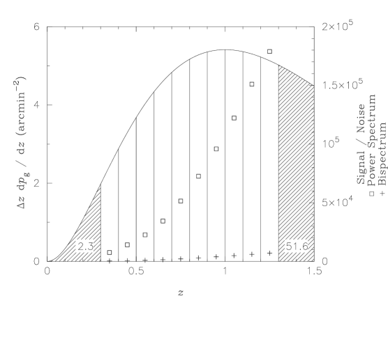
Figure 1: Galaxy redshift distribution and binning scheme employed in our analysis. The $y$-axis gives the number density of galaxies per redshift bin of width $\Delta z=0.1$. The numbers in the shaded regions indicate the unused galaxy number density in the low-$z$ and high-$z$ regions. The square symbols show the signal-to-noise for the power spectrum and the crosses for the bispectrum (see right side of the $y$-axis)

Since galaxy number is conserved, we may write

$$p_{\mathrm{g}}(\chi)\,\mathrm{d}\chi=p_{\mathrm{g}}(z)\,\mathrm{d}z.$$ (17)

Finally, we rewrite Eq. 14 as

$$P^{i}(l)=\frac{1}{(\bar{n}_{\mathrm{g}}^{i})^{2}}\int_{i}\mathrm{d}\chi\,\left[p_{\mathrm{g}}(z)\frac{\mathrm{d}z}{\mathrm{d}\chi}\right]^{2}\frac{1}{\chi^{2}}P_{\mathrm{g}}\left(\frac{l}{\chi},\ a\right),$$ (18)

where we have introduced the index $i$ to label the different redshift bins.

We calculate the full-sky bispectrum from the flat-sky bispectrum as

$$B_{l_{1}l_{2}l_{3}}\approx\left(\begin{array}[]{ccc}l_{1}&l_{2}&l_{3}\\ 0&0&0\end{array}\right)\sqrt{\frac{(2l_{1}+1)(2l_{2}+1)(2l_{3}+1)}{4\pi}}B(l_{1},l_{2},l_{3}),$$ (19)

with the flat-sky bispectrum likewise given by a Limber-style projection:

$$B^{i}(l_{1},l_{2},l_{3})=\frac{1}{(\bar{n}_{\mathrm{g}}^{i})^{3}}\int_{i}\mathrm{d}\chi\,\left[p_{\mathrm{g}}(z)\frac{\mathrm{d}z}{\mathrm{d}\chi}\right]^{3}\frac{1}{\chi^{4}}B_{\mathrm{g}}\left(\frac{l_{1}}{\chi},\frac{l_{2}}{\chi},\frac{l_{3}}{\chi},\ a\right).$$ (20)

To $O(\delta^{4})$, the galaxy bispectrum is given by the sum of two terms:

$$B_{\mathrm{g}}(k_{1},k_{2},k_{3},a) = b_{1}^{3}D^{4}(a)\left[2F_{2}(k_{1},k_{2})P(k_{1})P(k_{2})+\mathrm{cyclic}\ k_{i}\ \mathrm{permutations}\right]$$ (21)

$$+ \frac{1}{2}b_{1}^{2}b_{2}D^{4}(a)\left[2P(k_{1})P(k_{2})+\mathrm{cyclic}\ k_{i}\ \mathrm{permutations}\right],$$

where

$$F_{2}(k_{1},k_{2})=\frac{5}{7}+\frac{1}{2}\frac{\mn@boldsymbol{k}_{1}\cdot\mn@boldsymbol{k}_{2}}{k_{1}k_{2}}\left(\frac{k_{1}}{k_{2}}+\frac{k_{2}}{k_{1}}\right)+\frac{2}{7}\left(\frac{\mn@boldsymbol{k}_{1}\cdot\mn@boldsymbol{k}_{2}}{k_{1}k_{2}}\right)^{2}$$ (22)

is the second-order perturbation theory kernel. Note that the two terms have different triangle configuration dependence, and different dependence on $b_{1}$ and $b_{2}$.

2.3 Covariance and Fisher Matrix Formalism

The power spectrum covariance for redshift bin $i$ ignores the contribution from the trispectrum, which should be small in the linear regime:

$$C_{l,l^{\prime}}^{i}=\frac{1}{f_{\mathrm{sky}}}\frac{2}{2l+1}\left[P^{i}(l)+\frac{1}{\bar{n}_{\mathrm{g}}^{i}}\right]^{2}\delta_{ll^{\prime}}.$$ (23)

Here $f_{\mathrm{sky}}$ is the fraction of sky coverage for the survey, for which we use the value 0.1. $\bar{n}_{\mathrm{g}}^{i}$ is the galaxy density for redshift bin $i$. In our galaxy distribution (Fig. 1) it is 2.4 galaxies per arcmin² for the lowest redshift bin, and 5.4 galaxies per arcmin² at the peak of the galaxy distribution.

The bispectrum covariance ignores contributions from 3-, 4-, and 6-point functions, which are also expected to be small:

$$\begin{split}C_{l_{1}l_{2}l_{3},l^{\prime}_{1}l^{\prime}_{2}l^{\prime}_{3}}^{i}=&\frac{1}{f_{\mathrm{sky}}}\left[P(l_{1})+\frac{1}{\bar{n}_{\mathrm{g}}^{i}}\right]\left[P(l_{2})+\frac{1}{\bar{n}_{\mathrm{g}}^{i}}\right]\left[P(l_{3})+\frac{1}{\bar{n}_{\mathrm{g}}^{i}}\right]\\ &\times\big{(}\delta_{l_{1},l^{\prime}_{1}}\delta_{l_{2},l^{\prime}_{2}}\delta_{l_{3},l^{\prime}_{3}}+\delta_{l_{1},l^{\prime}_{1}}\delta_{l_{2},l^{\prime}_{3}}\delta_{l_{3},l^{\prime}_{2}}+\delta_{l_{1},l^{\prime}_{2}}\delta_{l_{2},l^{\prime}_{1}}\delta_{l_{3},l^{\prime}_{3}}+\delta_{l_{1},l^{\prime}_{2}}\delta_{l_{2},l^{\prime}_{3}}\delta_{l_{3},l^{\prime}_{1}}+\delta_{l_{1},l^{\prime}_{3}}\delta_{l_{2},l^{\prime}_{1}}\delta_{l_{3},l^{\prime}_{2}}+\delta_{l_{1},l^{\prime}_{3}}\delta_{l_{2},l^{\prime}_{2}}\delta_{l_{3},l^{\prime}_{1}}\big{)}.\end{split}$$ (24)

We assume that the likelihood function for the galaxy power spectrum and galaxy bispectrum is Gaussian, and employ a Fisher matrix analysis to approximate the likelihood near the fiducial cosmological model defined by the parameters in Table 1.

Parameter	Fiducial Value	Description	Calculated As
$\omega_{\mathrm{b}}$	0.023	Baryon Physical Density
$\omega_{\mathrm{d}}$	0.112	Dark-Matter Physical Density
$\Omega_{\mathrm{de}}$	0.69	Dark-Energy Density Parameter (Eq. 3)
$w_{0}$	-1	Equation of State Parameter (Eq. 2)
$w_{a}$	0	Equation of State Parameter (Eq. 2)
$A_{\mathrm{s}}$	0.82	Scalar Fluctuation Amplitude at $k=0.05/\mathrm{Mpc}$
$n_{\mathrm{s}}$	0.979	Primordial Spectral Index at $k=0.05/\mathrm{Mpc}$ (Eq. 11)
$\alpha$	0	Primordial Run ($=d\ln n_{\mathrm{s}}/d\ln k$) at $k=0.05/\mathrm{Mpc}$
$b_{1}$	0.998	First Order Galaxy Bias Factor (Eq. 10)
$b_{2}$	0	Second Order Galaxy Bias Factor (Eq. 10)
$\tau$	0.143	Optical Depth
$\Omega_{\mathrm{m}}$	0.31	Matter Density	$(\omega_{\mathrm{b}}+\omega_{\mathrm{d}})/h^{2}$
$\Omega_{\mathrm{b}}$	0.053	Baryon Density	$\omega_{\mathrm{b}}/h^{2}$
$\Omega_{\mathrm{tot}}$	1	Total Density (Assume Flat Cosmology)
$h$	0.66	Current Hubble Parameter in Units of 100 km / s / Mpc	$\sqrt{(\omega_{\mathrm{b}}+\omega_{\mathrm{d}})/(1-\Omega_{\mathrm{de}})}$
$\sigma_{8}$	0.88	Galaxy-Scale Fluctuation Amplitude

Table 1: The fiducial cosmological model used throughout this paper.

The Fisher matrix elements are given by

$$F_{\alpha\beta}^{P}=\sum_{i}\sum_{l_{\mathrm{min}}\leq l\leq l_{\mathrm{max}}}\frac{\partial P(l)}{\partial p_{\alpha}}(C_{l,l}^{i})^{-1}\frac{\partial P(l)}{\partial p_{\beta}}$$ (25)

for the power spectrum, and

$$F_{\alpha\beta}^{B}=\sum_{i}\sum_{l_{\mathrm{min}}\leq l_{1}\leq l_{2}\leq l_{3}\leq l_{\mathrm{max}}}\frac{\partial B_{l_{1}l_{2}l_{3}}}{\partial p_{\alpha}}(C_{l_{1}l_{2}l_{3},l_{1}l_{2}l_{3}}^{i})^{-1}\frac{\partial B_{l_{1}l_{2}l_{3}}}{\partial p_{\beta}}$$ (26)

for the bispectrum. The derivatives are evaluated at the fiducial model.

The large-scale limit, $l_{\mathrm{min}}$, is introduced because the Limber approximation fails when probing scales larger than the line-of-sight width of the given bin of galaxies. So we let $l_{\mathrm{min}}$ be the wavenumber that corresponds to the width of the bin. Since the information from baryon oscillations is contained at significantly larger $l$ in any case, this choice has little impact on our results.

The small-scale limit, $l_{\mathrm{max}}$, is meant to represent the scale beyond which perturbation theory is unacceptable. Nonlinear effects tend to smooth out the high-$l$ baryon oscillations in any case (Meiksin, White & Peacock Meiksin et al.1999). We define this (redshift-dependent) scale as $l_{\mathrm{max}}=k_{\mathrm{max}}/\chi(z)$, where $k_{\mathrm{max}}$ is defined by

$$\sigma^{2}=\int_{0}^{k_{\mathrm{max}}}\mathrm{d}^{3}k\,P(k)=1.$$ (27)

The values of $l_{\mathrm{max}}$ are plotted as the upper dotted line in Fig. 2. We will test below the sensitivity of our results to the choice of $l_{\mathrm{max}}$ by repeating our calculations for $l_{\mathrm{max}}/2$.

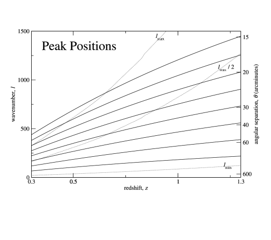
Figure 2: Angular separation and wavenumber of the first five peaks in the galaxy power spectrum induced by baryon oscillations as a function of galaxy redshift. The dotted lines correspond to our cutoff values $l_{\mathrm{max}}$ and $l_{\mathrm{min}}$. The $l(\theta)$ relation is approximate—we use $l=2\pi/\theta$.

We neglect the cross covariance between the power spectrum and bispectrum, which is proportional to the 5-point function, so that the Fisher information matrix for the power spectrum and bispectrum combined is simply the sum

$$F_{\alpha\beta}\approx F_{\alpha\beta}^{P}+F_{\alpha\beta}^{B}.$$ (28)

Finally, for a pair of parameters $p_{\alpha}$ and $p_{\beta}$, we calculate $\chi^{2}$ as

$$\chi_{p_{\alpha},p_{\beta}}^{2}=\left(\begin{array}[]{c}\Delta p_{\alpha}\\ \Delta p_{\beta}\end{array}\right)\left[\begin{array}[]{cc}\left(\mathbf{F}^{-1}\right)_{\alpha\alpha}&\left(\mathbf{F}^{-1}\right)_{\alpha\beta}\\ \left(\mathbf{F}^{-1}\right)_{\beta\alpha}&\left(\mathbf{F}^{-1}\right)_{\beta\beta}\end{array}\right]^{-1}\left(\begin{array}[]{c}\Delta p_{\alpha}\\ \Delta p_{\beta}\end{array}\right),$$ (29)

and identify the one-sigma contour as that contour defined by $\chi^{2}=2.3$.

For a flux-limited sample of galaxies, one should allow for a dependence of the galaxy bias on redshift. Hence we include an independent $b_{1}^{i}$ and $b_{2}^{i}$ for each redshift bin in our Fisher matrix.

We allow for biases in photometric redshifts by including the mean redshift of each galaxy bin as a nuisance parameter in the Fisher matrix. We set the rms in the mean redshift to be $0.01$ in $1+z$ for each redshift bin. This is conservative, since samples of spectroscopic redshifts will likely be available for calibration and the residual bias should be significantly smaller.

3 Results

3.1 Small Parameter Set

Since we are most interested in constraining the dark energy and galaxy bias, we first consider a restricted set of cosmological parameters: the dark-energy parameters, the overall amplitude normalization, and the bias parameters: $\{w_{0},w_{a},A_{s},b_{1},b_{2}\}$. We will impose no external priors on these parameters, but all other parameters are fixed to the fiducial values in Table 1 with the exception of $\Omega_{\mathrm{de}}$, which we marginalize over after applying a prior of 0.05. It is important to constrain $\Omega_{\mathrm{de}}$ to be able to extract information about the other parameters. Fortunately, CMB information can be used to constrain $\Omega_{\mathrm{de}}$ well. In the next subsection, we use a more complete set of parameters and combine our results with information from the CMB, and further allow for a possibly redshift-dependent galaxy bias by giving each redshift bin an independent $b_{1}^{i}$ and $b_{2}^{i}$.

Since the dark-energy parameters affect the angular diameter distances, they shift the position of the peaks in the projected galaxy power spectrum and bispectrum. In Fig. 3, we plot the angular galaxy power spectrum for our highest redshift bin: $1.2\leq z\leq 1.3$. Notice that, in addition to peak shifting, the overall amplitude of the fluctuations is also changed due to the growth factor’s dependence on dark energy. Because of this, we include those parameters that affect the amplitude of the galaxy statistics in our 5-parameter model. We neglect redshift uncertainties, and any redshift dependence of the bias parameters. That is, for this case, a single $b_{1}$ and $b_{2}$ parameter are used for all 10 redshift bins. Also, we plot the galaxy bispectrum signal in Fig. 4, which shows how these parameters modify the configuration dependence of the bispectrum.

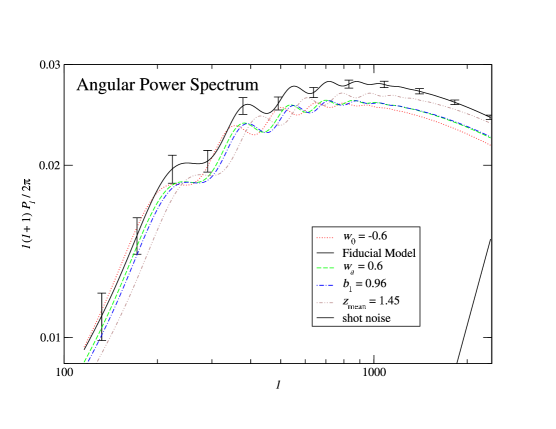
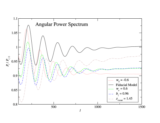
Figure 3: Effects of dark energy and other parameter variations on the projected galaxy power spectrum (Eq. 18). Except for the one labelled exception, we plot the projected power spectrum for our redshift bin with $z_{\mathrm{mean}}=1.25$. In the lower panel, we divide by a smooth spectrum corresponding to zero baryon density. This shows the differences between the models more clearly. Note that the shot noise curve for the lower redshift bins will be more than a factor of two larger than what is plotted here for $z=1.25$. Even so, it is clear that shot noise is not a significant source of error for the survey parameters we have used.

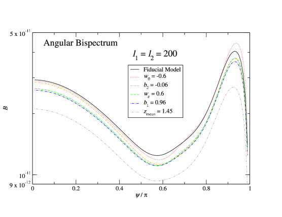
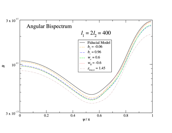
Figure 4: Configuration dependence of the projected bispectrum for various parameters choices as in Fig. 3. The upper panel uses equilateral triangles, while the lower panel uses isosceles triangles. Note that the effect of the bias parameter $b_{2}$, which leads to nonlinearity in the biasing, on the bispectrum is at the same level as that of $b_{1}$. Hence we expect that the bispectrum can be used to constrain this parameter.

The results of our Fisher matrix analysis for the 5-parameter model are presented in Fig. 5. These are two dimensional (marginalized) projections of 1-$\sigma$ contours in the 5-parameter space. Based on these contours, the addition of the bispectrum information does not appear to strengthen the dark-energy constraints substantially.

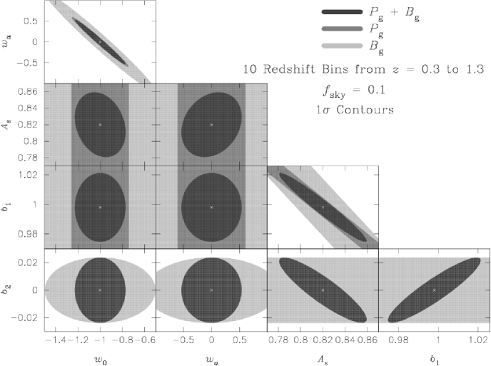
Figure 5: 1-$\sigma$ constraints from the Fisher matrix analysis of the 5-parameter cosmological model. The fiducial model is the cosmological constant model in Table 1, and is marked with an $\times$ in the figure.

However, constraints on the other three parameters are all significantly improved by the bispectrum information. This is not too surprising, for the galaxy power spectrum is proportional to $A_{\mathrm{s}}b_{1}^{2}$ (Eq. 18), and so the galaxy power spectrum alone cannot distinguish $A_{\mathrm{s}}$ and $b_{1}$. The degeneracy is broken by the bispectrum, as its dependence is $A_{\mathrm{s}}^{2}b_{1}^{3}$ (for $b_{2}=0$, Eq. 20). The degeneracy breaking is most dramatic in the $A_{\mathrm{s}}-b_{1}$ plot of Fig. 5, where the power spectrum or bispectrum information alone results in unbounded contours, but each contour comes with a different slopes, so that a tight contour is obtained when the two statistics are combined.

To lowest order in perturbation theory, the power spectrum does not depend on $b_{2}$. Dependence on $b_{2}$ enters at next order, proportional to the trispectrum. We have neglected the trispectrum contribution relative to the power spectrum, and so there are no power spectrum contours for $b_{2}$ in Fig. 18. However our formalism allows for this contribution to be included; with the bispectrum we can actually measure $b_{2}$ and then use the full power spectrum up to second order, which thus allows for a nonlinear, scale-dependent bias. The bispectrum enables constraints on $b_{2}$ because, as can be seen from Eq. 20, it contains two terms with different triangle configuration dependence. Only the second of the two terms depends on $b_{2}$, so observation of the galaxy bispectrum is useful to constrain this parameter.

3.2 Large Parameter Set

We have done the Fisher matrix analysis for a comprehensive set of cosmological parameters: $\{\omega_{\mathrm{b}},\omega_{\mathrm{d}},\Omega_{\mathrm{de}},w_{0},w_{a},A_{\mathrm{s}},n_{\mathrm{s}},\alpha,b_{1}^{i},b_{2}^{i},\tau\}$. Refer to Table 1 for a description of each parameter and its fiducial value. We use an independent pair of bias parameters for each redshift bin. We also include the mean redshift values of our redshift bins as additional nuisance parameters. We set the rms uncertainty to be $0.01$ in $1+z$ for the mean of each redshift bin.

To get a feel for the sensitivity of the power spectrum and bispectrum signals to each of these parameters, we have plotted in Fig. 6 and 7 the derivatives with respect to each parameter, evaluated at the fiducial model, as a function of $l$. The derivatives are weighted by a covariance factor, $1/\sqrt{C}$, as this is the weighting that enters the Fisher matrices (cf. Eqs. 25 and 26). Additionally, for the bispectrum signal, a sum over all triangle configurations should grant a proportionately higher sensitivity for larger $l$ values. We attempt to roughly account for this by weighting the bispectrum derivatives by a factor of $l^{2}$. Thus, squaring each weighted power spectrum and bispectrum derivative and summing is approximately (unmarginalized) $1/\sigma^{2}$ for that parameter.

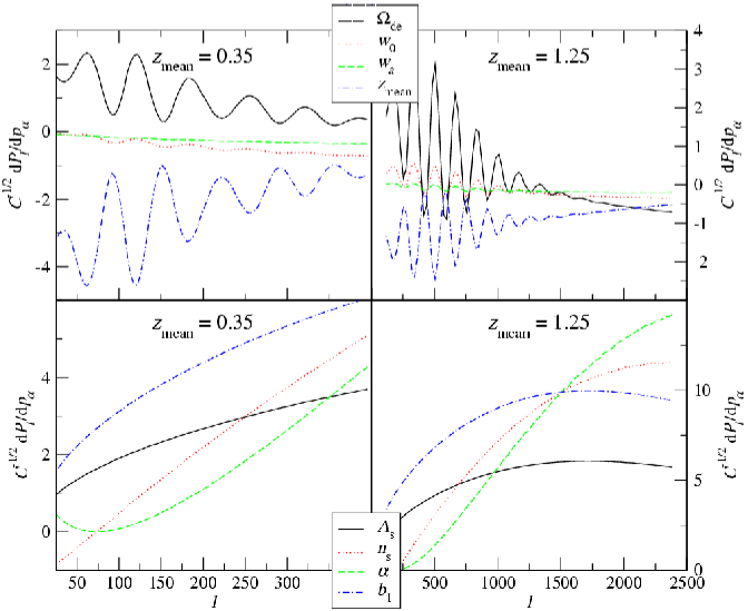
Figure 6: Plot indicating the sensitivity of the power spectrum to cosmological parameters as a function of $l$. The curves have been weighted by the covariance $1/\sqrt{C}$, as in Eq. 25.

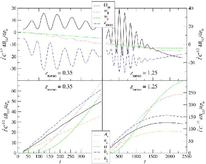
Figure 7: Plot indicating the sensitivity of the bispectrum to cosmological parameters as a function of $l$. The curves have been weighted by the covariance $1/\sqrt{C}$, as in Eq. 26, and by a factor of $l^{2}$ as an estimate of the number of triangle configurations.

With so many free parameters, it is necessary to apply some priors or to combine galaxy data with some complementary cosmological information, such as the CMB anisotropy. Galaxy information by itself suffers from strong degeneracies, like $w_{0}$-$w_{a}$ in particular. The marginalized one-sigma constraints from galaxy data alone are weak: $w_{0}$ constrained to $\pm 1$ and $w_{a}$ constrained to $\pm 4$. However, combination with the complementary CMB information gives interesting constraint ellipses, as shown in Fig. 8, or Table 2. We have not explored other possible cosmological probes with which to combine angular galaxy clustering.

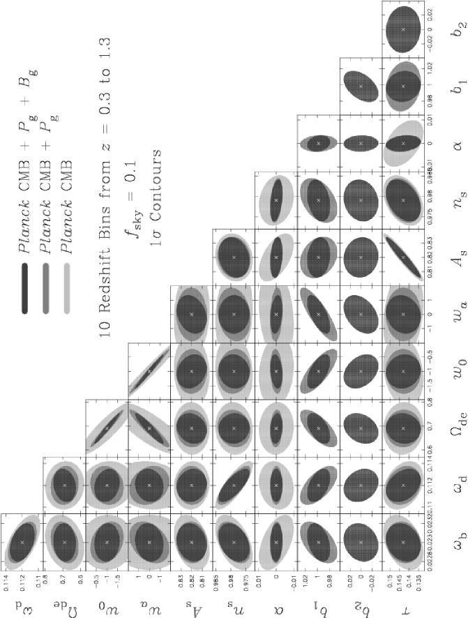
Figure 8: 1-$\sigma$ constraints from the Fisher matrix analysis of the 11-parameter cosmological model. We have combined our galaxy power spectrum and bispectrum Fisher matrices with a CMB Fisher matrix calculated using projected Planck covariances. The fiducial model is the cosmological constant model in Table 1, and is marked with an $\times$ in the figure.

We plot the one-sigma constraints obtained from our Fisher matrix analysis in Fig. 8. We calculate CMB Fisher matrices in the same way as was done for Takada & Jain (2004). CMB temperature and polarization power spectra and the cross spectrum are calculated using CMBFAST version 4.5 (Seljak & Zaldarriaga 1996). We assume the experimental specifications of the Planck 143 and 217 GHz channels with 65 per cent sky coverage. We also assume a spatially flat universe with no massive neutrinos and no gravity waves. We summarize our constraint prospects in Table 2.

parameter	$\mathrm{CMB}$		$\mathrm{CMB}+P_{\mathrm{g}}$		$\mathrm{CMB}+P_{\mathrm{g}}+B_{\mathrm{g}}$		$\mathrm{CMB}+\mathrm{SNe}$		$\mathrm{CMB}+\mathrm{SNe}+P_{\mathrm{g}}+B_{\mathrm{g}}$
$\omega_{\mathrm{b}}$	0.	00019	0.	00014	0.	00013	0.	00018	0.	00013
$\omega_{\mathrm{d}}$	0.	00145	0.	00116	0.	00099	0.	00141	0.	00096
$\Omega_{\mathrm{de}}$	0.	0727	0.	0520	0.	0421	0.	0061	0.	0044
$w_{0}$	0.	818	0.	511	0.	389	0.	077	0.	056
$w_{a}$	2.	180	1.	233	0.	881	0.	305	0.	223
$A_{\mathrm{s}}$	0.	0111	0.	0096	0.	0093	0.	0108	0.	0091
$n_{\mathrm{s}}$	0.	0041	0.	0036	0.	0034	0.	0039	0.	0034
$\alpha$	0.	0065	0.	0023	0.	0023	0.	0059	0.	0022
$b_{1}$			0.	0202	0.	0125			0.	0100
$b_{2}$					0.	021			0.	020
$\tau$	0.	0068	0.	0060	0.	0059	0.	0065	0.	0058

					SUGRA		SUGRA		SUGRA
parameter	$\mathrm{CMB}+P_{\mathrm{g}}^{z<2.3}$		$\mathrm{CMB}+P_{\mathrm{g}}^{z<2.3}+B_{\mathrm{g}}^{z<2.3}$		$\mathrm{CMB}+P_{\mathrm{g}}$		$\mathrm{CMB}+P_{\mathrm{g}}+B_{\mathrm{g}}$		$\mathrm{CMB}+\mathrm{SNe}$
$\omega_{\mathrm{b}}$	0.	00013	0.	00012	0.	00014	0.	00013	0.	00019
$\omega_{\mathrm{d}}$	0.	00094	0.	00075	0.	00123	0.	00096	0.	00150
$\Omega_{\mathrm{de}}$	0.	0439	0.	0361	0.	0064	0.	0062	0.	0061
$w_{0}$	0.	400	0.	311	0.	020	0.	020	0.	017
$w_{a}$	0.	941	0.	687	0.	038	0.	033	0.	038
$A_{\mathrm{s}}$	0.	0095	0.	0089	0.	0092	0.	0091	0.	0103
$n_{\mathrm{s}}$	0.	0033	0.	0031	0.	0038	0.	0034	0.	0041
$\alpha$	0.	0018	0.	0017	0.	0023	0.	0023	0.	0061
$b_{1}$	0.	0165	0.	0097	0.	0211	0.	0140
$b_{2}$			0.	020			0.	024
$\tau$	0.	0059	0.	0057	0.	0059	0.	0059	0.	0065

Table 2: Summary of marginalized 1-$\sigma$ prospects. Except where indicated otherwise, $P_{\mathrm{g}}$ and $B_{\mathrm{g}}$ include galaxies to redshift 1.3. The bias parameters listed here are those for the redshift bin with $0.9\leq z\leq 1.0$.

As in Fig. 5, the bispectrum helps primarily in constraining the amplitude and bias parameters. This is important because poor constraints on the $b_{1}$ and $b_{2}$ parameters mean that the dark-energy constraints may not be robust against possibly scale-dependent or nonlinear bias. The main difference in the level of accuracy achieved compared to the 5-parameter study is due to the bias parameters, since here we allow for two independent parameters in each redshift bin. Constraints on the biasing from other observations, or having some basis to reduce the parameter set from the twenty we use here, would improve dark-energy constraints by up to a factor of two.

Fig. 8 illustrates the power of a wide area multi-color survey, in that the full set of parameters gets constrained by the galaxy power spectrum and bispectrum, in conjunction with the CMB. For example, the constraints on the shape of the primordial power spectrum and on dark-energy parameters are interesting enough that increasing survey area or depth becomes appealing. We discuss these below.

We performed our analysis for a supergravity (SUGRA) inspired fiducial model, with $w_{0}=-0.82$ and $w_{a}=0.58$. A non-cosmological constant fiducial model results in stronger dark-energy constraints as a result of the redshift coverage of galaxy observations at relatively low redshift, and CMB observations at high redshift (Linder 2003). The comparison in Fig. 9 shows an improvement of over a factor of two in constraints on dark-energy parameters, though given Planck level CMB information galaxy clustering does not add much. Table 2 shows these results, as well as the use of Type Ia supernovae constraints at the level of SNAP.

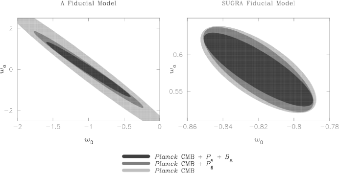
Figure 9: 1-$\sigma$ constraints from the Fisher matrix analysis of the 11-parameter cosmological model. The $\Lambda$-model is compared to the SUGRA model in the two panels. Note the difference in the range plotted for both parameters—the SUGRA model is constrained much better, though the galaxy statistics add less information to the CMB for this model.

4 Discussion

We have explored the prospects for obtaining interesting dark-energy constraints from the angular galaxy power spectrum and bispectrum. The use of the bispectrum adds some new information, though the signal-to-noise is significantly smaller than that of the power spectrum. However, its value lies in making dark-energy constraints robust against biasing features that cannot be measured with the power spectrum alone. We have shown that using the configuration dependence of the bispectrum, even a nonlinear, redshift-dependent bias characterized by 20 parameters in our study, can be measured and marginalized over.

The dark-energy constraints we obtain are weaker than those expected from Type Ia Supernovae or weak lensing. An ambitious spectroscopic survey could also do better by using three dimensional information (e.g. Seo & Eisenstein 2003; Linder 2003). However it is worth emphasising that our requirements of a multi-color imaging survey place no additional burdens over what is needed for weak lensing. Surveys such as the CFH Legacy survey are already in progress, and several larger surveys are planned for the future. We have made conservative choices of redshift binning and the maximum redshift used, to ensure that photometric redshift uncertainties would be well below the requirements. Thus we believe that, at the very least, the angular galaxy statistics would provide a useful independent check on dark-energy constraints from imaging surveys. As discussed below, it is possible to improve the constraints to levels competitive with the methods mentioned above by increasing survey area, depth and quality of photometric redshifts.

High redshift ($z\sim 1$) galaxies are important to obtain the parameter constraints at the level advertised here. This is true for several reasons. The linear regime extends to smaller scales at higher redshifts because nonlinear evolution progresses to larger scales over time. This is evident from Fig 2, which demonstrates that, at higher redshifts, a greater number of the baryon-induced peaks lie in the linear region. The three dimensional nonlinear scale, $k_{\mathrm{max}}$, is a factor of two smaller at $z=1.3$ than at $z=0.3$. Further, the two-dimensional nonlinear scale, $l_{\mathrm{max}}$, depends not only on $k_{\mathrm{max}}$, but also on the angular diameter distance, which for $z=1.3$ is a factor of 3 larger than at $z=0.3$. For ongoing and future deep imaging surveys the number density of galaxies in these higher redshifts bins is larger. This is helpful in that we can select special classes of galaxies with useful properties, such as the luminous red galaxies studied from the Sloan Digital Sky Survey. Even if they are a small fraction of the galaxy population, the shot noise contribution is not likely to be a limiting factor as discussed above and by Seo & Eisenstein (2003).

Since we wish to learn about the time dependence of the dark-energy equation of state, it is important to sample our statistics over a wide enough range in redshift. In particular, for the equation of state we have used, which is linear in the scale factor, the degeneracy between $w_{0}$ and $w_{a}$ is broken by sampling galaxies over several redshift bins across a range of redshifts. This is illustrated in Fig. 10 and Fig. 11, where the marginalized 1-$\sigma$ constraints for the dark-energy parameters are plotted as a function of survey redshift depth. The constraints from a survey that extends to $z\simeq 2$ are twice as good as one that goes to $z\simeq 0.5$.

Figure 10: The two panels show the dependence of dark-energy constraints on survey depth and area. The left panel shows constraints in the $w_{a}$-$w_{0}$ plane for different values of the maximum redshift bin used for the analysis. The right panel shows constraints for different survey areas, given by the values of the sky fraction, $f_{\mathrm{sky}}$.

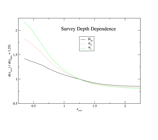
Figure 11: Dark-energy parameter constraints as a function of the depth of the galaxy survey. These use the galaxy power spectrum and bispectrum combined with CMB data at the level of Planck. The curves are normalized to the constraints expected for a survey with nominal depth of $z=1.25$.

The right panel of Fig. 10 shows the dependence of dark-energy constraints on survey area. While the errors do not scale simply with $f_{\mathrm{sky}}$ due to the use of CMB priors, there is a significant improvement with every factor of two in sky coverage. Using Fig. 10, our fiducial values can be scaled to a range of survey depths and areas.

The ability to use the deep imaging capability of future surveys to go well beyond $z\sim 1$ will depend in part on the accuracy of the photometric redshifts. With low enough scatter in these and even a very small sub-sample of spectroscopic redshifts for calibration, the methods we have explored can provide much better constraints on dark-energy models, especially models with a larger component of the dark-energy density at higher redshifts. As discussed by Seo & Eisenstein (2003), the requirements on photometric redshift scatter are not severe: an rms of $0.04$ in $1+z$ is adequate. Here we have further checked that residual biases in the mean redshift of each bin do not significantly degrade dark-energy constraints (see Fig. 12). Hence it is not unreasonable to hope that the innermost contour of Fig. 10, corresponding to the highest redshift bin at $z=2.25$, will be achievable for a high quality survey. In addition, a smaller rms in the photometric redshifts will mean that we can use effectively smaller redshift bins to improve the constraints. A rigorous analysis of redshift binning would require the use of cross-spectra and their covariances; alternatively, the galaxy distribution could be treated as three dimensional, with large errors in the redshift coordinate (Seo & Eisenstein 2003).

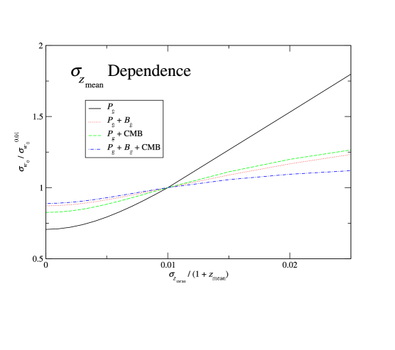
Figure 12: Dependence of the $w_{0}$ constraint on the uncertainty in the redshift bin centers. Plotted is $\sigma_{w_{0}}$ normalized to the fiducial value (rms error of $0.01$ in $1+z$). These use the galaxy power spectrum and bispectrum combined with CMB data at the level of Planck.

Besides the baryon oscillation features, dark-energy parameters affect the overall shape and amplitude of the angular power spectrum and bispectrum. To separate the effects of the oscillations, we calculated galaxy Fisher matrices using the “no-wiggles” transfer function of Eisenstein & Hu (1998). If we use just the galaxy clustering information, the constraints for the no-wiggles case are about twice as large. With CMB priors, the effect is smaller as the CMB enables the amplitude of the spectra to also provide information. We do still have a standard ruler in the no-wiggles case: the peak in the power spectrum corresponding to matter-radiation equality (Cooray et al. 2001). The physical length scale of this ruler is set at decoupling by $\omega_{m}$, which can be well constrained by the CMB. Hence the broad shape of the power spectrum adds information on angular diameter distances. The amplitude depends on the bias parameter and the growth factor, which is sensitive to the dark energy. Using both the galaxy power spectrum and bispectrum with the CMB, the scalar amplitude $A_{\mathrm{s}}$, the two bias parameters, $b_{1},b_{2}$, and the power spectrum amplitude in each redshift bin, are constrained sufficiently well.

We have tested our choices of fiducial bias parameters and the quasi-linear regime. We repeated our analysis by setting $l_{\mathrm{max}}$ to half the value used, and find that it leads to a 6–11 per cent degradation in the dark-energy constraints for galaxy plus CMB information. Thus our results are not very sensitive to the choice of cutoff of the quasi-linear regime and the neglect of non-Gaussian contributions to the covariances.

Since one of the goals of our formalism is to allow for a nontrivial biasing of the galaxies, we also performed our analysis with $b_{2}=1$ as the fiducial value, thus allowing for a nonlinear term in the biasing. It led to improved constraints on most parameters due to a larger impact of adding bispectrum information, e.g. the 1-$\sigma$ uncertainty in the dark-energy parameters was lower by 10 per cent. More importantly, we find that $b_{2}$ can be measured sufficiently well for a wide range of fiducial values, so that an effectively nonlinear, scale-dependent bias can be consistently incorporated in our analysis. This validates our conclusion that bias and dark-energy constraints can be simultaneously obtained by using the bispectrum. An alternate approach to galaxy biasing and other properties is to use the halo model, which may also enable us to probe smaller scales, as discussed in Hu & Jain (2003). The analytical models for the bispectrum need to checked and calibrated with $N$-body simulations. A large number of independent realizations would be needed since the covariances in the bispectra need to be accurately measured as well.

References

- Bernardeau et al. (2002) Bernardeau, F., Colombi, S., Gaztañaga, E., Scoccimarro, R., 2002, Phys. Rep., 367, 1.
- Blake & Glazebrook (2003) Blake, C., Glazebrook, K., 2003, ApJ, 594, 665.
- Budavari et al. (2003) Budavari, T., et al., 2003, ApJ, 595, 59.
- Caldwell et al. (1999) Caldwell, R. R., Dave, R., Steinhardt, P. J., 1999, Phys. Rev. Lett., 80, 1582.
- Cooray et al. (2001) Cooray, A., Hu, W., Huterer, D., Joffre, M., 2001, ApJ, 557, L7.
- Connolly et al. (2002) Connolly, A., et al., 2002, ApJ, 579, 48.
- Eisenstein (2003) Eisenstein, D. J., in “Wide Field Multi-Object Spectroscopy”, 2003, ASP Conference Proceedings, ed. A. Dey, 35.
- Eisenstein & Hu (1998) Eisenstein, D. J., Hu, W., 1998, ApJ, 496, 605.
- Feldman et al. (2001) Feldman, H. A., Frieman, J. A., Fry, J. N., Scoccimarro, 2001, Phys. Rev. Lett., 86, 1434.
- Frieman & Gaztanaga (1999) Frieman, J. A., Gaztanaga, E., 1999, ApJ, 521, L83.
- Fry (1999) Fry, J. N., 1994, Phys. Rev. Lett., 73, 215.
- Hu (2002) Hu, W., Phys. Rev. D., 2002, 65, 023003.
- Hu & Haiman (2003) Hu, W., Haiman, Z., Phys. Rev. D., 2003, 68, 063004.
- Hu & Jain (2003) Hu, W., Jain, B., 2003, astro-ph/0312395.
- Huterer (2002) Huterer, D., Phys. Rev. D., 2002, 65, 3001.
- Kosowsky & Turner (1995) Kosowsky, A., Turner, M. S., 1995, Phys. Rev. D, 52, 1739.
- Linder (2003) Linder, E., 2003, Phys. Rev. D, 68, 083504.
- Linder & Jenkins (2003) Linder, E., Jenkins, A., 2003, MNRAS, 346, 573.
- Ma et al. (2000) Ma, C. P., Caldwell, R. R., Bode, P., Wang, L., 1999, ApJ, 521, L1.
- Matsubara & Szalay (2003) Matsubara, T., Szalay, A., 2003, Phys. Rev. Lett., 90, 021302.
- (21) Meiksin, A., White, M., Peacock, J. A., 1999, MNRAS, 304, 851.
- Mobasher et al. (2004) Mobasher, B., et al., 2004, ApJ, 600, L167.
- Perlmutter et al. (1999) Perlmutter, S., et. al., 1999, ApJ, 517, 565.
- Pope et al. (2004) Pope, A., et. al., 2004, ApJ, 607, 655.
- Riess et al. (1998) Riess, A. G., et. al., 1998, AnJ, 116, 1009.
- Riess et al. (2001) Riess, A. G., et. al., 2001, ApJ, 560, 49.
- Seo & Eisenstein (2003) Seo, H. J., Eisenstein, D., 2003, ApJ, 598, 720.
- Seljak & Zaldarriaga (1996) Seljak, U., Zaldarriaga, M., 1996, ApJ, 469, 437.
- Spergel et al. (2003) Spergel, D. N., et al., 2003, ApJS, 148, 175.
- Takada & Jain (2004) Takada, M., Jain, B., 2004, MNRAS, 348, 897.
- Tegmark et al. (2004) Tegmark, M., et. al, 2004, Phys. Rev. D., 69, 103501.
- Tonry et al. (2003) Tonry, J. L., et. al., 2003, ApJ, 594, 1.
- Verde et al. (2002) Verde, L., et al., 2002, MNRAS, 335, 432.
- Wang & Steinhardt (1998) Wang, L., Steinhardt, P. J., 1998, ApJ, 508, 483.