Models of the giant quadruple quasar SDSS J1004+4112

Abstract

SDSS J1004+4112 is an unprecedented object. It looks much like several quadruple quasars lensed by individual galaxies, only it is $\sim 10$ times larger, and the lens is a cluster dominated by dark matter. We present free-form reconstructions of the lens using recently-developed methods. The projected cluster mass profile is consistent with being shallow, $r^{-0.3...-0.5}$, and can be fit with either an NFW or a flat-cored 3 dimensional mass distribution. However, we cannot rule out projected profiles as steep as $r^{-1.3}$. The projected mass within $100{\rm\,kpc}$ is well-constrained as $(5\pm 1)\times 10^{13}M_{\odot}$, consistent with previous simpler models. Unlike previous work, however, we are able to detect structures in the lens associated with cluster galaxies. We estimate the mass associated with these galaxies, and show that they contribute not more than about 10% of the total cluster mass within $100{\rm\,kpc}$. Typical galaxy masses, combined with typical luminosities yield a rough estimate of their mass-to-light ratio, which is in the single digits. Finally, we discuss implications for time-delay measurements in this system, and possibilities for a partial Einstein ring.

1 Introduction

At the present time about 30 quadruply imaged QSO systems are known (Kochanek et al., 2004). The majority of these are lensed by individual galaxies, sometimes aided by a nearby group or cluster. Given the typical masses of galaxies one expects that the typical image separation would be around 1 second of arc. This is borne out in the data. The exceptions, i.e. large separation lenses are rare, and have to be produced by groups or clusters, not isolated galaxies. In fact, the very first multiply imaged system, Q0957+561A,B (Walsh et al., 1979) is a cluster lens with two of its images separated by $\sim 6^{\prime\prime}$. The recently discovered SDSS J1004+4112 (hereafter J1004+411) is the first system where a galaxy cluster, $z=0.68$, splits a background QSO, $z=1.734$, into four images, producing an unprecedented image separation of $\sim 14^{\prime\prime}$ (Inada et al., 2003). While this is the first such system to be discovered, Oguri et al. (2004) estimate that the full Sloan Digital Sky Survey will yield several similar large separation QSO lenses.

The image configuration of J1004+411 is almost identical to the first-known quad PG1115+080 (if we swap NE and SW) but the scale is $\sim 10$ times larger, hence our description of J1004+411 as a giant quadruple quasar. The giantness prompts us to ask: is this cluster lens just a scaled-up version of a typical galaxy lens, or is it fundamentally different? We will answer this question by constructing and studying ensembles of pixelated mass maps for J1004+411 and comparing them with analogous mass maps for PG1115+080.

Oguri et al. (2004; hereafter O4) have modeled the system in various configurations of a main galaxy, cluster halo, and external shear. Even though a wide range of mass distributions is consistent with the lensing data, a few general conclusions apply to most mass models. For example, the mass in the vicinity of the images is elongated North-South, consistent with the distribution of visible galaxies. On larger scales, i.e. well outside the image ring, the cluster’s mass distribution must be such that it gives rise to a large shear. O4 also conclude that the cluster’s center must be offset from that of the brightest galaxy by several kiloparsec. In the rest of the paper we model the J1004+411 cluster-lens in detail. We agree with most of the general conclusions reached by O4, even though our modeling method is very different from theirs. Unlike the parametric modeling in O4, our modeling allows us to detect the mass inhomogeneities in the cluster associated with the individual galaxies.

2 Modeling the cluster

Before making any actual models, it is helpful to use lensing theory to identify qualitative features of the lens that are model independent. As argued in Saha & Williams (2003), examining the lens morphology already provides useful information. In Figure 1 we show the inferred configuration of the saddle-point contours for J1004+411, assuming the lens is centered on the dominant galaxy, called G1 in Oguri et al. (2004; hereafter O4). The images are labeled according their inferred time order. [A different configuration with the reverse time-ordering is also possible, but very unlikely. We will consider it in section 6.] As evident from the contours, images 1 and 2 are minima while 3 and 4 are saddle-points. Since time delays scale with the area of the lens (Saha, 2004) the expected time delays would be $\sim 100$ times longer than in PG1115+080. But apart from its giant size the lens appears to be a typical inclined quad. The long axis would be roughly N-S and the source somewhat SW of the lens center.

Figure 1: Expected image morphology and time-ordering of the images, assuming the center of the lens is coincident with the center of the dominant galaxy.

To reconstruct the lens we use the PixeLens code (Saha & Williams, 2004). The input to PixeLens are (i) the lensing data, which for J1004+411 are the positions of images 1–4 relative to the cluster center, and the redshifts of the lens and source, and (ii) a chosen prior, which we explain below. The output is an ensemble of pixelated mass maps, which we then preprocess in various ways. Each model in the ensemble reproduces the lens data precisely, and so does any normalized superposition of models in the ensemble. Since superposition of many individual maps reinforces common features of mass maps, and diminishes random ‘one-time’ features, the ensemble-average map can be interpreted as a smoothed map of the inner portion of the cluster. Uncertainties are readily derived from the statistics of the ensemble. Each ensemble presented in this paper has 500 models.

Earlier implementations of free-form lens reconstruction have been applied to the famous lensing clusters A370 and A2218 (AbdelSalam et al., 1998a, b) and the galaxy lenses PG1115+080, B1608+656, and B1422+231 (Saha & Williams, 1997; Williams & Saha, 2000; Raychaudhury et al., 2003). PixeLens itself was developed for galaxy lenses, but it can be used without change for J1004+411. In fact, because in J1004+411 there are a number of cluster galaxies in the vicinity of the images, making the mass distribution lumpy, free-form modeling is even more desirable than in galaxy lenses. Free-form modeling also has the advantage of not requiring that an artificial (and unphysical) distinction be made between individual galaxies and cluster halo, before modeling.

If only the primary constraints from lensing are used, the ensemble will be dominated by mass maps that are highly irregular and have spurious extra images. Restricting the ensemble to lenses that could plausibly be galaxies or clusters is achieved by secondary constraints, or a prior. PixeLens priors have six kinds of constraints, as follows.

1. Mass pixels are non-negative: $\kappa\geq 0$.

2. Inversion symmetry about the lens center can be imposed as an option. Since J1004+411 appears to be an asymmetric lens we will not apply this constraint.

3. The lens must be centrally concentrated. PixeLens implements this by restricting the direction of the local density gradient, $\phi_{\scriptscriptstyle\nabla}$. The default is $\phi_{\scriptscriptstyle\nabla}\leq 45^{\circ}$, meaning that the density gradient must point within $45^{\circ}$ degrees of the center. A very small allowed range such as $\phi_{\scriptscriptstyle\nabla}\leq 8^{\circ}$ forces the average mass distribution to be more nearly circular. A very large allowed range like $\phi_{\scriptscriptstyle\nabla}\leq 80^{\circ}$ tends to result in mass “fingers” emanating from the lens center, making the mass map look nothing like a galaxy or cluster.

4. The $\kappa$ of any pixel can be at most twice the average of its neighbors: $\kappa\leq 2\,\langle\kappa_{\rm nbr}\rangle$, ensuring smoothness of mass maps. (But the central pixel is not constrained in this way, to allow for a density cusp.) This is the default setting. Weakening or removing this constraint altogether will allow for more substructure.

5. The slope of the radial mass profile, or $\alpha$ in $r^{-\alpha}$ is bounded. The default is $\alpha\geq 0.5$. Note that $\alpha$ is defined here for the projected mass profile; hence an isothermal has $\alpha=1$.

6. Finally, PixeLens has an optional constant external shear, and the prior confines its allowed directions, but not its magnitude. We denote the shear direction by $\phi_{\gamma}$. For $\phi_{\gamma}=0^{\circ}$ the shear will have PA along the north-south axis, and because of the way shear is defined in lensing theory that corresponds to external mass along the east-west direction.

In the following, we present results using four different priors.

Prior A1: $$\phi_{\scriptscriptstyle\nabla}\leq 45^{\circ},\quad 0.25\leq\alpha\leq 3,\quad\phi_{\gamma}=70^{\circ}\pm 45^{\circ}.$$

Prior A2: $$\phi_{\scriptscriptstyle\nabla}\leq 45^{\circ},\quad 0.25\leq\alpha\leq 3,\quad\phi_{\gamma}=10^{\circ}\pm 45^{\circ}.$$

Prior B1: $$\phi_{\scriptscriptstyle\nabla}\leq 8^{\circ},\quad 0.25\leq\alpha\leq 3,\quad\phi_{\gamma}=70^{\circ}\pm 45^{\circ}.$$

Prior B2: $$\phi_{\scriptscriptstyle\nabla}\leq 8^{\circ},\quad 0.25\leq\alpha\leq 3,\quad\phi_{\gamma}=10^{\circ}\pm 45^{\circ}.$$

All the above priors are somewhat different from the default PixeLens settings. The lower bound on the steepness constraint, $\alpha$ has been relaxed, since the central region of the cluster can be shallower than $\alpha=0.5$; profiles steeper than 3 are unrealistic, and have been excluded. The A and B-type priors differ in their gradient constraints, $\phi_{\scriptscriptstyle\nabla}$. In this paper we are particularly interested in recovering mass associated with cluster galaxies, and other possible substructures in the lens. These substructures are just the deviations from the smooth circularly symmetric mass profile (see Section 5). Therefore, two of our priors (B1 and B2) were chosen to have a small range of allowed $\phi_{\scriptscriptstyle\nabla}$ angles. Priors A1 and A2 adopt the default setting for $\phi_{\scriptscriptstyle\nabla}$. The smoothness constraint has been removed altogether from both types of priors. This was done to facilitate the recovery of substructure: a localized mass lump can, in principle, be more pronounced than the default smoothness constraint allows for.

Dropping the smoothness constraint produces a lot of pixel-to-pixel fluctuations, which do not completely die down even if 500 individual maps are co-added. To reduce these fluctuations we smooth the final ensemble-average map with a filter that spreads part of each pixel onto its eight neighbors with weights corresponding to a Gaussian with $\sigma=\sqrt{0.5}$ pixel, or $\approx 0.67^{\prime\prime}$.

The external shear directions, $\phi_{\gamma}$, were set as follows. A1 and B1 require the external shear to correspond roughly to the local alignment of galaxies, those within about $60^{\prime\prime}$ of the lens (see Fig. 13a of O4), while A2 and B2 have shear aligned similar to the typical shear direction in the models by O4. If A2/B2 are correct the shear would arise well outside of the central $\sim 30^{\prime\prime}$–$60^{\prime\prime}$ of the lens.

3 Maps of the total mass

The four panels of Figure 2 show reconstructions using the priors A1, A2, B1 and B2. The solid dots are the QSO images, while crosses mark the locations of cluster galaxies.

Let us consider first the top panels in Fig. 2 (i.e., A1 and A2 priors). Evidently, pre-specifying the approximate direction of external shear affects the shape of the mass distribution to some degree; the most notable difference between right and left panels is the extent of the SW elongation of isodensity contours. The presence of a mass component in the W part of the map is to some degree degenerate with external shear direction $\phi_{\gamma}=10^{\circ}$. This probably explains why the SW extension is rather pronounced in A1 ($\phi_{\gamma}=70^{\circ}$) and almost absent in A2 ($\phi_{\gamma}=10^{\circ}$).

More interestingly, we see that even though we did not tell PixeLens anything about individual galaxies, their presence is clearly reflected in the reconstructed mass distributions. (Crosses in the figure represent locations of galaxies.) The density contours encompass the northern grouping of galaxies, and also indicate the presence of mass just south east of the lens center. There are several galaxies there, inside as well as outside the image circle. The mass distribution in the very central region of the cluster, within the radius of the innermost image, is probably not well constrained and the two galaxies just west of the central one are not noticeable. The slight extension of the density contours towards SW are probably due to the 2–3 galaxies located in that area, just beyond the image circle.

The maps in the bottom panels (priors B1 and B2) also indicate the presence of the galaxy groupings in the N and SE parts of the map, however, here the distortions of the isodensity contours are very slight: one can tell that the contours are not entirely circular by comparing them to the dotted thin circles drawn through the locations of the images, to guide the eye. The near circular nature of the isodensity contours is a direct consequence of restricting the range of the direction of density gradient to a narrow cone ($\phi_{\scriptscriptstyle\nabla}\leq 8^{\circ}$). In Section  5 we will discuss, in more detail, how well B1 and B2 maps recover the presence of galaxies in the cluster.

Figure 2: Mass maps using different priors as indicated. Contours are $\kappa=0.1,0.2,0.4,\ldots,3.2$ in logarithmic steps. The reconstruction window has radius $15.2^{\prime\prime}$, the sky scale being $\simeq 7.5\rm\,kpc/arcsec$. In each panel the mass maps shown are averages from ensembles of 500; additional smoothing has been applied to the maps using $\sigma=0.67^{\prime\prime}$ (see Section 2). Crosses are galaxies with $i<24$, taken from Fig. 13a of O4. Thin dotted circles are cluster-centered circles drawn through the images, to guide the eye.

4 Gradient of the mass profile

The mass distribution in dark matter halos is of great importance in determining the nature of dark matter. In the central regions of clusters, $\sim 50$–$100{\rm\,kpc}$, the baryons are less important than in the central regions of individual galaxies, therefore one can reasonably assume that the best-fit density profile is due to dark matter alone. In fact, our analysis in Section 5 will allow us to test this assumption, at least partially: we will estimate the fraction of mass associated with individual cluster galaxies, but we cannot say anything about hot diffuse smoothly distributed gas that might be present in the cluster.

From our free-form mass maps, we derive the mass enclosed within a given radius, $M(<r)$. The four panels of Figure 3 show $M(<r)$ for the four cases shown in Fig. 2; dashed lines are 90% confidence limits obtained using the whole ensemble of individual recovered mass maps. (Note that the uncertainties at different $r$ are not independent.) As is typical of quads, the total mass within the image circle is very well constrained, and the errors are smallest where $\langle\kappa(<r)\rangle=1$. But because of the mass-disk degeneracy (Falco et al., 1985; Saha, 2000) the distribution of the mass can take on various forms. We expect that the envelope delineated by the confidence limits would look like two curves crossing at $\langle\kappa(<r)\rangle=1$, where the two intersecting curves of the envelope represent the shallowest and the steepest mass profiles possible. This is borne out in the plots.

Even though the density slopes from A-type and B-type priors are very different the mass enclosed within $\sim 60{\rm\,kpc}$, which is the average radius of the image annulus, is nearly identical in all four cases, emphasizing again the robustness of enclosed mass estimate.

Figure 3: Enclosed mass $M(<r)$ in terasol (or $10^{12}M_{\odot}$). In each panel, the thick solid line is the ensemble-median of $M(<r)$, with the dashed lines enclosing 90% of the individual models in the ensemble. The four short vertical bars at the bottom mark the image radii; the images 2 and 3 being nearly equidistant from the lens center, their positions are almost indistinguishable in this plot. The number in parenthesis is the projected double logarithmic density slope $\alpha$, while the dotted line represents the isothermal slope, $\alpha=1$. The two thin lines in the upper right panel are some specific NFW (solid) and CORE (dot-dash) fits, see Section 4 for details.

The thin dotted line in each panel of Fig. 3 corresponds to the isothermal slope, or $\alpha=1$. The actual value of $\alpha$ in the image annulus is shown in parenthesis. Comparing panels we see that the derived slope depends strongly on the secondary constraint assumptions (whether an A-type or B-type prior was used) but A1/A2 and B1/B2 give similar slopes.

Since A-type and B-type priors result in such different density slopes for J1004+411, is the derived density slope simply a consequence of the prior, with the true density slope unrecoverable? Comparison with the galaxy lens PG1115+080 indicates that the situation is not that dire. While A-type and B-type priors in the case of J1004+411 result in $\alpha\approx 1.3$ and $0.4$, respectively, the same set of priors when applied to PG1115+080 (but using $\phi_{\gamma}=-45^{\circ}\pm 45^{\circ}$ appropriate for this lens) result in $\alpha\approx 1.6$ and $1.2$. Comparing the two sets of numbers suggests that the galaxy in PG1115+080 has a steeper density profile than does the cluster in J1004+411. To test this hypothesis we apply another prior, with a narrow range of shallow density slopes: $0.3\leq\alpha\leq 0.5$. If $\phi_{\scriptscriptstyle\nabla}\leq 8^{\circ}$ PixeLens finds no mass models that satisfy this set of constraints for PG1115+080, and if $\phi_{\scriptscriptstyle\nabla}\leq 45^{\circ}$ ensemble mass maps have spurious images. It seems that shallow slopes are incompatible with PG1115+080. For J1004+411 PixeLens has no problem generating realistic mass maps using shallow density profiles, and either type of $\phi_{\scriptscriptstyle\nabla}$ constraints. We conclude that the density gradient in PG1115+080 is around $1$–$2$, while J1004+411 is shallower, possibly as shallow as $\alpha\approx 0.3$. It may be possible to improve these constraints by testing against a large number of synthetic models, analogous to the blind tests in Williams & Saha (2000) but much more detailed; we leave that for the future.

It is interesting to note that B-type priors result in much better constrained $M(<r)$ distributions (Fig. 3) than A-type priors. This is probably due to steeper density profiles (as result from A-type priors) being more vulnerable to mass disk degeneracy, and conversely, shallower profiles resulting from B-type priors leaving little room for mass disk degeneracy.

Since $M(<r)$ is a circularly averaged quantity, it can be used to constrain ‘average’ halo density profile models. To do this we fit two types of density profiles: (i) $\rho\propto(1+r/r_{c})^{-\gamma}$ having a flat density core (called ‘CORE’ models), and (ii) NFW  (Navarro, Frenk & White, 1997), with $\rho\propto[(r/r_{s})(1+r/r_{s})^{2}]^{-1}$. In the latter case, scale radius, $r_{s}$, and virial radius, $r_{200}$, are related through the concentration parameter, $c=r_{200}/r_{s}$, and take on values of about 4–5 for rich galaxy clusters.

The goodness of fit of NFW/CORE models will be ascertained using $\chi^{2}$, which requires rms values. The distribution of $M(<r)$ values for any given $r$ for an ensemble of models is not necessarily Gaussian, and is often asymmetric, but for the purposes of estimating rms of the distribution we assume that the size of the 90% error-bars (which we obtain from PixeLens) is 1.65 times the size of the 68% error-bars, the latter being $1\sigma$ for a Gaussian. We use these estimates of $\sigma$ to calculate $\chi^{2}$ for the model fits. The $\chi^{2}$ contour levels using A2 and B2 mass maps are shown in Fig. 4, but A1 and B1 maps would have produced similar results. The plotted $\chi^{2}$ contour levels are indicated in the figure caption, however, these values are not to be taken too seriously because our assumption of symmetric, Gaussian distributed errors is not always very good. The non-smoothness of some contours in these plots is partly due to that.

The top panels of Fig. 4 show the $\chi^{2}$ contours when CORE and NFW density models are fitted to the enclosed mass data of A2 prior models. These density distributions are rather steep, so neither CORE nor NFW provide very good fits. Some of the better CORE and NFW fits (marked with a cross in each of the two top panels) are plotted in the top right panel of Fig. 3 with thin dot-dash and solid lines, respectively. The CORE model requires the density outside of the central $\sim 30$ kpc to be very steep, $\alpha=4$, while NFW fit has a concentration parameter of $c\approx 30$, well outside the typical range for galaxy clusters. Thus, A2 prior mass models seem to be unrealistic.

The bottom panels of Fig. 4 show the $\chi^{2}$ contours when CORE and NFW density models are fitted to the enclosed mass data of B2 prior models. These density distributions are shallow, and could easily accommodate flat density cores as large as 100 kpc. The two crosses in the bottom left panel mark some specific models; if the corresponding models were plotted in the bottom right panel of Fig. 3 they would be indistinguishable from the actual line representing $M(<r)$; we did not overplot these. The thin lines in the bottom right panel (NFW fits) show contours of constant virial radius of NFW halos. The virial radius, and hence the mass of the best fitting halos are relatively well constrained; $r_{200}\approx$ 1–1.5 kpc. The halo marked with a cross provides an excellent fit to the data. This halo’s concentration parameter is $c=5$, and its mass is $M_{200}\approx 4.17\times 10^{14}M_{\odot}$, which is comparable to the mass estimated by O4,  3.1–4.6$\times 10^{14}h_{65}^{-1}M_{\odot}$.

Figure 4: Simple parametric fits to free-form mass maps generated using A2 (top panels) and B2 (bottom panels) priors. The fits are derived via the enclosed mass, and solid lines are contours of constant $\chi^{2}$. Left panels show CORE models of the form $\rho\propto(1+r/r_{c})^{-\gamma}$; $\chi^{2}$ contours are at 1, 3, 5, 10, 30 per dof. Right panels show NFW model fits where concentration parameter and scale radius were allowed to vary independently; $\chi^{2}$ contours are at 10, 100, 1000, 10000 per dof. The $\chi^{2}$ increase very rapidly away from the locus of best-fit NFW models; for example, the model marked with a cross in the bottom right panel has a $\chi^{2}\approx 1.5$. (The ‘islands’ are artifacts of the grid and should be disregarded.) The crosses in all four panels show models mentioned in Section 4. The thin lines in the two right panels are curves of constant virial radius, $r_{200}$ (or, equivalently constant halo mass); $r_{200}=1.5,1,0.5$ Mpc from top to bottom.

We conclude that our fits, using B2 prior models, to the circularly averaged density distribution of the cluster are very similar to those in O4. But our free-form models can be taken much further than parametric models, revealing the deviations from the average density profile, i.e., substructure in the mass distribution.

5 Detecting substructure

The term ‘substructure’ encompasses a host of different types of deviations of the lensing mass distribution from smooth. There is compact substructure, like stars or globular clusters in galaxies, and smooth substructure, like dwarf dark matter halos around galaxies. Compact substructure can result in micro- and/or milli-lensing, whereby many unresolved micro- and milli-images are produced. Micro-lensing and milli-lensing lead to a wealth of observable consequences (Wambsganss, 1990; Schechter & Wambsganss, 2002; Williams & Saha, 1995) some of which are yet to be detected.

Smooth mass lumps in the main lens do not split the macro-images into sub-images, but they can affect the fluxes, and even the positions of macro-images. Observed flux ratios of macro-images have been extensively used in the recent literature to look for smooth substructure in and around galaxies (Dalal & Kochanek, 2002; Metcalf & Zhao, 2002; Chiba, 2002; Evans & Witt, 2003).

Here, we look for substructure using positions of macro-images only. To our knowledge, this is the first work to do so. Also, our macro-lens is a cluster of galaxies, not an individual galaxy as is the case in most flux-ratio substructure investigations, hence the mass range of substructure lumps that we find (see below) is necessarily larger than that searched for in individual galaxies.

To examine the substructure in the central regions of J1004+411, at every point in the map we subtract the circularly averaged surface mass density for that radius (i.e. distance from cluster center), and thus obtain a residual mass map.

Figure 5 shows the residual mass distributions corresponding to the mass maps in Figure 2. All four reconstructions detect the main substructure components in the cluster: the galaxy group N of image 4, and the galaxy group SE of images 2 and 3. The only galaxy which is consistently under-detected is one $\sim 2^{\prime\prime}$ W of center; this is probably because the galaxy is well inside the region of lensing constraints, therefore it is not clear how much stock we should put into the central features of the map. It might at first be surprising that given the smoothness and near circular appearance of the iso-density contours in the bottom panels of Fig 2, the substructure in the bottom panels of Fig. 5 is very well delineated. The explanation lies in the shallow average density profile of B-type prior maps: it is easy to ‘hide’ substructure superimposed on a nearly flat density field.

The most obvious difference between A1 and A2, and similarly between B1 and B2 is the presence of a mass lump in the SW part of the A1 and B1 maps. This mass component does not correspond to any visible galaxies. The simplest explanation is that A1 and B1 assume the wrong external shear direction ($\phi_{\gamma}=70^{\circ}\pm 45^{\circ}$), while the shear direction incorporated into the A2 and B2 priors ($\phi_{\gamma}=10^{\circ}\pm 45^{\circ}$) is close to the true one. The latter is the same shear direction as obtained in O4. A2 and B2 maps have no extended mass features that do not correspond to visible galaxies. From now on we will concentrate mainly on the A2 and B2 prior models.

Having now a good visual match to the galaxies in the residual mass maps, we test the substructure more quantitatively. Let us define $M_{l}({\theta\kern 2.58334pt\raise 6.88889pt\hbox to0.0pt{\hss$\scriptstyle\rightarrow$}\kern-0.86108pt})$ as the residual mass within $l$ pixels of a point ${\theta\kern 2.58334pt\raise 6.88889pt\hbox to0.0pt{\hss$\scriptstyle\rightarrow$}\kern-0.86108pt}$ of the residual mass map A2 or B2. Then a choice of points $\{{\theta\kern 2.58334pt\raise 6.88889pt\hbox to0.0pt{\hss$\scriptstyle\rightarrow$}\kern-0.86108pt\!\!_{n}}\}$ will result in a distribution $\{M_{l}({\theta\kern 2.58334pt\raise 6.88889pt\hbox to0.0pt{\hss$\scriptstyle\rightarrow$}\kern-0.86108pt\!\!_{n}})\}$. If the mass residuals are uncorrelated with the galaxies (the null hypothesis), then the distribution of $\{M_{l}({\theta\kern 2.58334pt\raise 6.88889pt\hbox to0.0pt{\hss$\scriptstyle\rightarrow$}\kern-0.86108pt\!\!_{n}})\}$, where ${\theta\kern 2.58334pt\raise 6.88889pt\hbox to0.0pt{\hss$\scriptstyle\rightarrow$}\kern-0.86108pt\!\!_{n}}$ are galaxy positions should not be significantly different from the $\{M_{l}({\theta\kern 2.58334pt\raise 6.88889pt\hbox to0.0pt{\hss$\scriptstyle\rightarrow$}\kern-0.86108pt\!\!_{n}})\}$ distribution obtained using random ${\theta\kern 2.58334pt\raise 6.88889pt\hbox to0.0pt{\hss$\scriptstyle\rightarrow$}\kern-0.86108pt\!\!_{n}}$ positions. Using the 19 galaxies with $i<24$ taken from O4’s Fig. 13a, we find that a Kolmogorov-Smirnov test rejects the null hypothesis at significance levels of 99.92%, 99.91%, 99.75%, 95.8% confidence levels, for $l=2,4,6,8$ respectively, for A2 prior model. For B2, the corresponding confidence levels are 99.28%, 99.37%, 97.2%, 98.94%. Thus, we unambiguously detect mass associated with galaxies in cluster J1004+411.

It should also be possible to infer the typical size of the galaxies, but because the galaxies are heavily clustered, especially in the N part of the cluster, we can only estimate an approximate upper limit on size. We define upper limit as the size corresponding to the $l$ value above which the enclosed residual mass summed over all galaxies begins to decrease. This corresponds to 4 pixels, or $\sim 30{\rm\,kpc}$, for both A2 and B2.

We can also estimate the mass associated with the cluster galaxies, by adding up the residual mass of all pixels that lie within $l$ pixels of all 19 galaxies and then multiplying by 2 as a rough correction for the fact that residual mass can be negative or positive. For $l=1$ and $l=4$, the average mass per galaxy is $1.2\times 10^{11}\,M_{\odot}$ and $1.9\times 10^{11}\,M_{\odot}$ respectively, for A2, and $2.1\times 10^{10}\,M_{\odot}$ and $5.1\times 10^{10}\,M_{\odot}$ for B2 prior model. For a 64-fold change in galaxy volume, there is only a $\sim 2$-fold change in the derived average galaxy mass, for both priors. This small change must be partly due to the galaxies being heavily clustered, but it also indicates that the derived mass is quite robust.

From the photometry presented in O4 (see their Fig. 10) we estimate that a typical galaxy (of the 19 closest to the images), has $M_{r}\sim-20.5$, or about $1.6\times 10^{10}~{}L_{\odot}$. Taking a typical galaxy mass to correspond to the mass enclosed within the 4 pixels, we obtain M/L ratios of 11.2 and 3.2, for A2 and B2 respectively. This is compatible with the galaxies in the center of the cluster being composed entirely of stars. Since we know the total enclosed mass in the reconstructed region, and the total mass of the galaxies, we can estimate the fraction of mass contained in the galaxies; this comes to about 9%, and 2% for A2 and B2 respectively. This is also the lower limit on the baryonic content of the inner $100{\rm\,kpc}$ of the cluster; we have no means of determining the mass in hot diffuse smoothly distributed gas in the cluster.

The values of M/L ratios and mass fraction in galaxies derived using priors A2 and B2 can be interpreted as defining the range of uncertainty in these quantities. We found further PixeLens reconstructions using different sets of priors to be generally consistent with this interpretation.

Figure 5: Residuals after subtracting off the circularly averaged density profile in each panel of Figure 2. The thick contour is now $\Delta\kappa=0$, the thin solid lines are $\Delta\kappa=0.025,0.05,0.1,0.2,\ldots$ and the thin dotted lines are $\Delta\kappa=-0.025,-0.05,-0.1,-0.2,\ldots$ Crosses mark the positions of galaxies with $i<24$.

If J1004+411 is indeed a scaled-up version of a galaxy lens like PG1115+080, the implications are interesting. If the latter system has $\sim$2–10% of its mass in the same type of substructure as J1004+411, we would expect to detect a total mass of $(0.6-3)\times 10^{10}\,M_{\odot}$ distributed in several individual lumps of $\sim 10^{9}\,M_{\odot}$. Although we would not detect individual lumps, their expected mass range is typical of dwarf dark matter halos currently being searched for around individual galaxies.

Accordingly, we reconstruct PG1115+080 in a way as similar as possible to our reconstruction of J1004+411: we use an A and B-type priors (with $\phi_{\gamma}=-45^{\circ}\pm 45^{\circ}$ appropriate for PG1115+080), allow the lens to be asymmetric, and disregard the observed time delays, supplying PixeLens only the image positions. The resulting maps are shown in Fig. 6. It is clear that the mass distribution in PG1115+080 is considerably smoother than that of the corresponding maps of J1004+411, except for the central region. Also, the map is very nearly inversion-symmetric, unlike J1004+411. This result indicates that the halo of PG1115+080 is not populated with numerous dwarf dark matter halos. Comparison of the residual maps also removes any remaining concerns that our detection of substructure in J1004+411 could be an artifact.

Figure 6: Results from models of PG1115+080 using A (left panels) and B-type (right panels) priors, and $\phi_{\gamma}=-45^{\circ}\pm 45^{\circ}$. Upper: mass maps analogous to Figure 2. Lower: residual mass maps analogous to Figure 5.

6 Time delay predictions

In a model-ensemble generated by PixeLens, each model has a set of time delays. An ensemble of time delays is conveniently plotted as a histogram and immediately provides predicted time delays and uncertainties.

Nearly all the models in O4 have the time-ordering shown in Figure 1, but a few have the reverse ordering. We can reproduce the reverse time-order, and the appropriately modified version of Figure 1, if we assume the lens center is $\simeq 3^{\prime\prime}$ SW of the dominant galaxy. (We do not know whether a similar offset applies in the O4 models, but expect it is probably the case.) But shifting the lens center also tends to allow a lot of models with spurious extra images. Hence the reverse time-order seems very unlikely, and we will not consider it further.

Figure 7 shows the distribution of predicted time delays between different images for the models of the B2 prior, which give shallow mass profiles for the cluster, similar to those of O4. The possible range of time-delays is large, but the spread is similar to other quads—see e.g., Raychaudhury et al. (2003). Apart from the scale, the predicted time delays are as one would expect for galaxy lenses. The time delays for the A2 prior models (not shown) are about 4 times longer than those for B2, as would be expected for the deeper potential wells of the A2 models.

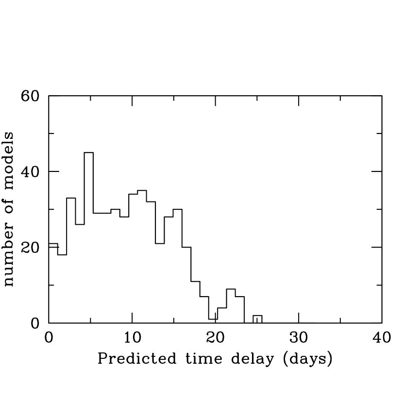
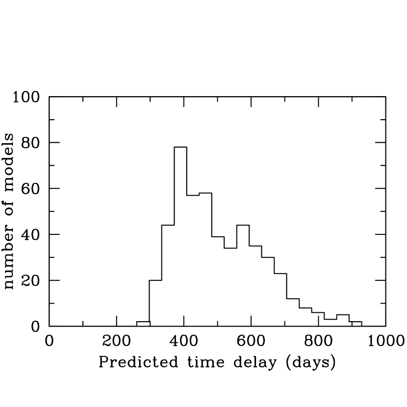
Figure 7: Predicted time delays for J1004+411, from reconstructions using a B2 prior. Upper left: images 2–3, upper right: 1–4, lower left: 1–2, lower right: 3–4.

The parametric models by O4 show a similar range of predicted time delays (see their Fig. 19), with the typical delays for 2–3 and 1–4 image pairs comparable to what we have for B-prior reconstructions of J1004+411 (upper panels of Fig. 7). Interestingly, their models also show a strong correlation between the 2–3 and 1–4 time delays (i.e., the shortest and longest). An easy way to look for such a correlation using PixeLens is simply to fix one of the time delays. Accordingly, we fixed the shortest time delay at 10 days and generated another ensemble of models. Figure 8 shows the 1–2 and 3–4 time delays with the extra constraint. We see that the spread gets smaller but not very much smaller.

Figure 8: Like the two lower panels of Figure 7, but with the 2–3 delay fixed at 10 days.

Comparing the time-delay results leads to an interesting point regarding parametric versus free-form lens models. Time delays varying over a large range while staying in the same ratio are a signature of the mass-disk degeneracy, which makes lens models steeper while lengthening all time delays uniformly—see Saha (2000) for details of this simple interpretation. Other lensing degeneracies do not necessarily share this property. Thus we conclude that the O4 models are exploring the mass-disk or steepness degeneracy very well, but are much more restricted with regard to other degeneracies. On the other hand, in PixeLens the mass-disk degeneracy, though important, is no longer dominant.

Even though it would not strongly constrain the lens, a measurement of the 2–3 time delay in J1004+411 would be very interesting for three reasons. First, it would test the inferred time-ordering. Second, time delays between close pairs of images are not normally measurable—in galaxy lenses they would be less than a day—only in J1004+411 the giant scale brings the delay to a convenient length. On the other hand, the longer time delays, which in galaxy lenses are more practical to measure, in J1004+411 would be several years and hence much more difficult to measure. Third, a 2–3 time-delay measurement would be a test of the relatively shallow mass profile. The shallow profiles from B2 priors predict a delay of $\sim 10$ days, whereas the steeper models from A2 priors give time delays of $\sim 50$ days.

7 A ring in J1004+411?

Lenses with small deviations from circular symmetry produce the best rings; B1938+666 being the best example (King et al., 1998). Asymmetric and lumpy lenses produces short ring segments only, so J1004+411 is not expected to be much of a spectacle in that regard. Nevertheless, a partial ring is possible. In Figure 9 we show partial rings such as would be produced by a source (host galaxy) with a conical light profile of radius $2^{\prime\prime}$ with the A2 and B2 priors. It is really the arrival-time surface of the QSO with closely-spaced contours, but it mimics a ring through a surprising side-effect of lensing theory (Saha & Williams, 2001). The width of the ring depends on the steepness of the density profile of the lens; for the same source, the steep profile of A2 model results in a narrow ring, while the much shallower profile of B2 gives rise to a wider ring.

Prominent partial rings such as in those in Figure 9 would require a large host galaxy. That seems unlikely, probably an incipient ring in the form of arc-like features around the QSO images is more to be expected.

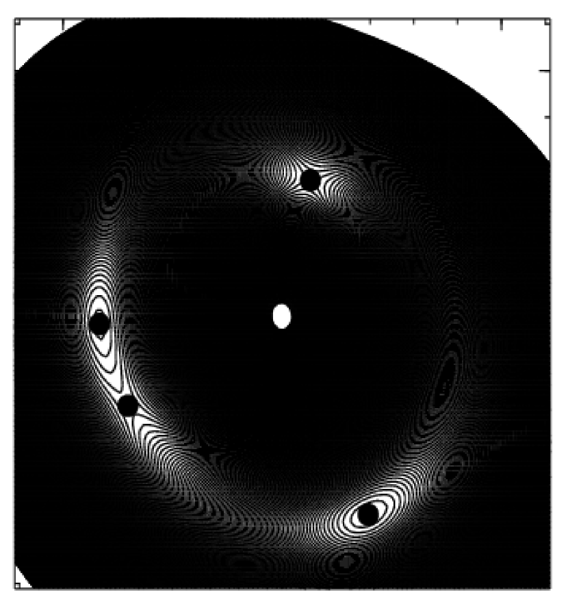
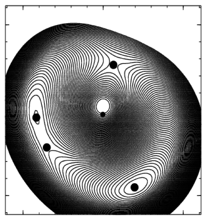
Figure 9: Predicted ring, assuming the quasar host galaxy has a conical profile of radius $\sim 2^{\prime\prime}$. Upper and lower panels are for A2 and B2 prior models, respectively.

8 Conclusions

Although physically a cluster lens, J1004+411 is very like a Brobdingnagian version of a galaxy lens like PG1115+080, with image separations $\sim 10$ larger and the expected time delays $\sim 100$ times longer. Thus the 2–3 time delay goes from hours to weeks while the 1–2 and 3–4 time delays go from weeks to years, an interesting reversal of what is observationally most accessible. We argue that unless the QSO host galaxy is rather large an Einstein ring is not expected in J1004+411, but a partial ring is very likely.

The projected mass enclosed by the lens is very well constrained as $\approx 2.5\times 10^{13}M_{\odot}$ within $60{\rm\,kpc}$, and $\approx 5.5\times 10^{13}M_{\odot}$ within $100{\rm\,kpc}$. The circularly averaged density profile is well fit by NFW halos, a virial mass of $\approx 4.2\times 10^{14}M_{\odot}$ being quite robust but the concentration parameter being uncertain. Density profiles with flat central cores of $r_{c}<100{\rm\,kpc}$ are not excluded.

Thus far our results are similar to those of O4, who used a combination of parametric descriptions of the central galaxy, cluster, and external shear to model QSO image positions.

Our most interesting new result, however, is the detection of structure in the lens, i.e. deviations of the mass distribution in the cluster from smooth. We detect the structure using image positions (not flux ratios) as model input. The structure in J1004+411 is clearly associated with cluster galaxies, as confirmed by a KS test. A “control” analysis of PG1115+080 reveals no analogous structures. Although our mass maps cannot detect individual cluster galaxies (partly because they are so heavily clustered), we can still estimate their mass content, which comprises about 2%–10% of cluster mass. This implies typical galaxy mass-to-light ratios of about $3-11$, and indicates that dark matter in the inner region of the cluster is mostly not bound to individual galaxies.

References

- AbdelSalam et al. (1998b) AbdelSalam, H.M., Saha, P., & Williams, L.L.R., 1998, AJ, 116, 1541
- AbdelSalam et al. (1998a) AbdelSalam, H.M., Saha, P., & Williams, L.L.R., 1998, MNRAS, 294, 734
- Chiba (2002) Chiba, M. 2002, ApJ, 565, 17
- Dalal & Kochanek (2002) Dalal, N., & Kochanek, C.S. 2002, ApJ, 572, 25
- Evans & Witt (2003) Evans, N.W.E, & Witt, H.J. 2003, MNRAS, 345, 1351
- Falco et al. (1985) Falco, E.E., Gorenstein, M.V. & Shapiro, I.I. 1985, ApJ, 289, L1
- Inada et al. (2003) Inada et al 2003, Nature, 426, 810
- King et al. (1998) King, L.J. et al. 1998, MNRAS, 295, L41
- Kochanek et al. (2004) Kochanek, C.S., Falco, E.E., Impey, C., Lehar, J., McLeod, B. & Rix, H.-W. 2004, CASTLES Survey, http://cfa-www.harvard.edu/glensdata/
- Metcalf & Zhao (2002) Metcalf, R.B., & Zhao, H.-S., 2002, ApJ, 567, L5
- Navarro, Frenk & White (1997) Navarro, J.F., Frenk, C.S., & White, S.D.M. 1997, ApJ, 490, 493