Evolution of the Dependence of Rest-frame Color and Morphology Distribution on Stellar Mass for Galaxies in the Hubble Deep Field North

Abstract

Using the Subaru very deep $K^{\prime}$-band imaging and HST WFPC2/NICMOS archival data of the Hubble Deep Field North, we investigate the evolution of the stellar mass, color, morphology of galaxies to $z\sim 3$. We mainly examine the rest-frame $U-V$ color distribution of galaxies as a function of stellar mass. At $0.3\lesssim z\lesssim 2$, galaxies seem to be divided into the two populations at around the stellar mass of $\sim 5\times 10^{9}$ M_⊙. The low-mass galaxies have relatively bluer rest $U-V$ color and their color does not show clear correlation with stellar mass over the range of 10⁸–5$\times$10⁹M_⊙. On the other hand, at higher mass, the more massive galaxies tend to have the redder $U-V$ color. The average $U-V$ color of the low-mass galaxies becomes bluer gradually with redshift, from $U-V\sim 0.2$ at $z\sim 0.5$ to $U-V\sim-0.2$ at $z\sim 2$. On the contrary, the correlation between the stellar mass and rest $U-V$ color of the high-mass population does not seem to change significantly between $z\sim 0.3$ and $z\sim 2$. The morphological distribution shows that at $z\lesssim 1$, the low-mass population is dominated by disk galaxies, while the fraction of early-type galaxies is larger in the high-mass population. At $1<z<2$, although the fraction of irregular galaxies increases, the similar trend is observed. At $z>2$, it is seen that more massive galaxies tend to have redder $U-V$ color over the range of $10^{9}$-$10^{10}$M_⊙, although we can only sample the galaxies with stellar mass larger than $\sim 1\times 10^{9}$M_⊙. These results suggests that the star formation history of galaxies depends on their stellar mass very much. The low-mass population is likely to have relatively long star formation timescale, and their formation redshifts do not seem to be much higher than $z\sim 2$ under the assumption of constant star formation rate. At the stellar mass larger than $\sim 5\times 10^{9}$M_⊙, there must be some mechanisms which suppress the star formation in galaxies at $0<z<2$.

1 Introduction

For the study of the galaxy formation in the framework of the structure formation of the universe, it is important to investigate the various properties of galaxies as a function of their mass. Unlike color or morphology, since the dynamical or stellar mass is relatively unaffected by recent star formation activities or the morphological transformation processes such as interactions or mergers, which increase mass at most factor of two, it can be conveniently used as independent variable for the investigation of the star formation history or the evolution of the morphology distribution of galaxies. While the dynamical mass is more directly connected to the prediction of the structure formation theory, the stellar mass can be more easily measured using the NIR luminosity with optical-NIR colors or spectral stellar population indices (e.g, Giallongo et al., 1998; Brinchmann & Ellis, 2000; Kauffmann et al., 2003). Since the stellar mass of galaxies reflects the past history of star formation, its evolution is closely related to the time when the majority of stars in those galaxies built up. Thus the investigations of the distribution of various properties of galaxies as a function of stellar mass at various epochs help our understanding of the processes of galaxy formation and evolution.

For local universe, Kauffmann et al. (2003) investigated the stellar mass dependence of the star formation history, sizes, and structural parameter of galaxies with the Sloan Digital Sky Survey data, and found that galaxies divide into two distinct families at a stellar mass of 3$\times 10^{10}$M_⊙. These families are found to have different star formation activities, morphologies, surface mass densities, and so on.

At intermediate redshifts, Giallongo et al. (1998) estimated the stellar mass of galaxies with $R^{\prime}<25$ in the field of the $z=4.7$ quasar BR 1202-0725 using the $BVrIK$ imaging data. They found that the distribution of the stellar mass of galaxies at $z=0.4$-0.8 has a median value of $\sim 5\times 10^{8}$M_⊙, but the blue galaxies with $B^{\prime}-V^{\prime}\leq 1.4$ show a narrower and peaky stellar mass distribution at $\sim 10^{8}$M_⊙, and the all galaxies with M${}_{stellar}>2\times 10^{9}$M_⊙ have $B^{\prime}-V^{\prime}>1.4$. Brinchmann & Ellis (2000) derived the stellar mass of $I<22$ galaxies with spectroscopic redshifts in the CFRS and LDSS surveys using the optical–NIR photometries, and investigated their relation with morphology or star formation rate. They found that in the range of $10.5<\log{{\rm M}_{stellar}}<11.6$, the comoving stellar mass density in irregular galaxies increases rapidly from $z\sim 0.2$ to $z\sim 1.0$, and this is complemented by the modest decrease of the mass density in spheroidal galaxies. They also pointed out that at $0.2<z<1.0$, the more massive galaxies tend to have lower specific star formation rate R$=$SFR/M_stellar.

For galaxies at $z>2$, Sawicki & Yee (1998) investigated the broad-band optical–NIR SED of Lyman break galaxies with spectroscopic redshifts in the Hubble Deep Field North (HDF-N), and found that their stellar masses are about 1/15 of a present-day L^∗ galaxy and that these galaxies are dominated by very young ($\lesssim 0.2$Gyr) stellar population. Papovich, Dickinson, & Ferguson (2001) also investigated the spectral stellar population properties of those galaxies with spectroscopic redshifts in the HDF-N, using the optical–NIR HST imaging data. They found that the Lyman break galaxies with “L${}^{*}_{\rm LBG}$” UV luminosity have the stellar mass of roughly 1/10 of a present-day L^∗ galaxy ($\sim 10^{10}$M_⊙), and they are well fitted by the model with population ages that range from 30 Myr to 1 Gyr. Fontana et al. (2003) estimated the stellar mass of $z>2$ galaxies with $K<25$ using the HDF-S optical–NIR imaging data. In addition to the star forming galaxies, they found that there are a few red galaxies at $z\gtrsim 2$, and that the fraction of older objects seems to increase at large stellar mass, although the biases against old/passive objects exist near the detection limit. Shapley et al. (2001) investigated the stellar mass of relatively bright $R<25.5$ Lyman break galaxies at $z\sim 3$, using $UGRIK$-bands photometries. They found that their $R-K$ color distribution is wide-spread, and their UV luminosity (both dust-corrected and uncorrected) is uncorrelated with the estimated stellar mass.

On the other hand, several studies indicate that the morphological sequence of galaxies seen in the present universe seems to be formed between $z\sim 1$ and $z\sim 3$ (e.g., Dickinson, 2000; Kajisawa & Yamada, 2001). The possible rapid evolution of cosmological stellar mass density at $1<z<3$ is also reported (Dickinson, Papovich, Ferguson, & Budavári, 2003; Fontana et al., 2003). Therefore it is interesting to investigate the evolution of the mass dependence of these properties of galaxies back to such an important epoch for galaxy formation.

In this paper, in order to understand the formation and evolution of field galaxies, we investigate the rest-frame color and morphological distribution of galaxies in the Hubble Deep Field North as a function of stellar mass back to $z\sim 3$, using the archival HST WFPC2/NICMOS data and the very deep Subaru/CISCO $K^{\prime}$-band imaging. Deep $U$-to-$K$ band images allow us to investigate these properties of galaxies at the rest-frame $V$-band toward $z\sim 3$, and estimate the rest $U-V$ color without extrapolation. The $U-V$ color is relatively sensitive to the average age of their stars because it covers the wavelength region where the largest features in galaxy continuum spectra at near-UV to optical wavelengths, namely, a 4000 Å break and/or the Balmer discontinuity exist. The wide wavelength coverage also help us to constrain the stellar mass of galaxies with relatively high accuracy. In section 2, we describe the data reduction and the sample selection, and the way to estimate the stellar mass, rest-frame color, and morphology of our sample. We investigate the evolution of the rest-frame $U-V$ color and morphological distribution of galaxies as a function of stellar mass in section 3. A discussion of these results is presented in section 4. In section 5, we summarize the results obtained from our analysis. We use the standard (Vega) magnitude system throughout the paper. HST filter bands refer to F300W, F450W, F606W, F814W, F110W, F160W bands as $U_{300}$, $B_{450}$, $V_{606}$, $I_{814}$, $J_{110}$, $H_{160}$, respectively.

2 Data Reduction and Sample Selection

2.1 CISCO $K^{\prime}$-band data

The HDF-N field was observed at the $K^{\prime}$-band with the Subaru telescope equipped with the Cooled Infrared Spectrograph and Camera for OHS (CISCO, Motohara et al., 2002) on 2001 April 3 and 4. The detector used was a 1024 $\times$ 1024 HgCdTe array with a pixel scale of 0.111 arcsec for the Optical Nasmyth secondary, which provides a field of view of $114^{\prime\prime}\times 114^{\prime\prime}$. A number of dis-registered images with short exposures (20 s for each frame) were taken in a circular dither pattern with a $10$ arcsec diameter. A series of twelve frames were taken at each place and the telescope was then moved to the next position. The position of each cycle (12 $\times$ 10 frames) was randomly dithered with about $10$ arcsec offset. The total exposure time was 36740 sec, about 10 hours. The weather condition was stable during the observations, and seeing was between 0.3 and 0.7 arcsec, typically $\sim$ 0.5 arcsec.

The data were reduced using the IRAF software package. There was a variation in the dark level of CISCO, which depends on the sky background level. At first, we thus performed flat-fielding using the superflat frame for CISCO $K^{\prime}$-band data (Motohara et al., 2002), and measured the background level of each frame. Then, “sky background $+$ dark” frame for each image was produced from the sample of frames with nearly same background level, and the sky $+$ dark subtraction was performed. Further we subtracted the residual background by fitting the frames with 5th-order surface function. Then source detection was done for each frame and the offsets between frames were measured. These frames were co-registered and combined. We then performed tentative source detection for this combined frame to make the mask image. Using this mask image, we masked objects in each raw frame, and remade “sky background $+$ dark” frame, which is less affected by the fluctuation due to bright objects than the first version, for each raw frame. Thereafter the same procedures were done to make the second-version combined image. From second-version combined image, the mask image was made again. Three iterations of these procedures were performed to make final combined image. Figure 1 shows the combined CISCO $K^{\prime}$-band image of the HDF-N.

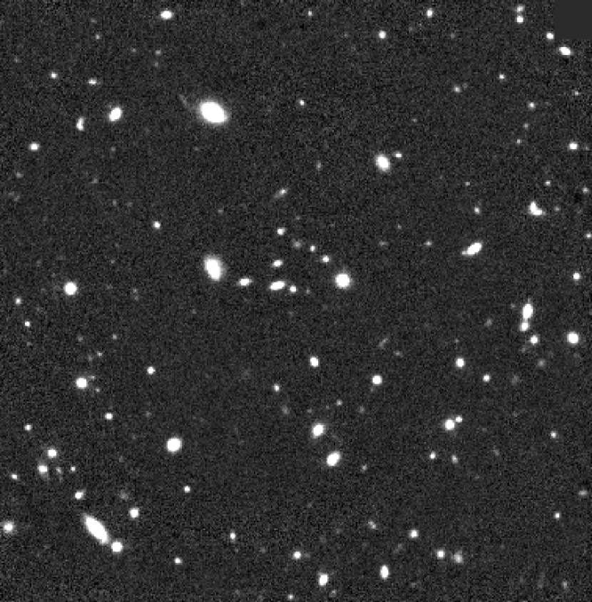
Figure 1: CISCO $K^{\prime}$-band image of the Hubble Deep Field North.

The FWHM of the point sources in the final combined image is about 0.55 arcsec. Since the field of view of the final image is about $110^{\prime\prime}\times 110^{\prime\prime}$, this $K^{\prime}$-band image is not completely covered the whole HDF-N area (Figure 2).

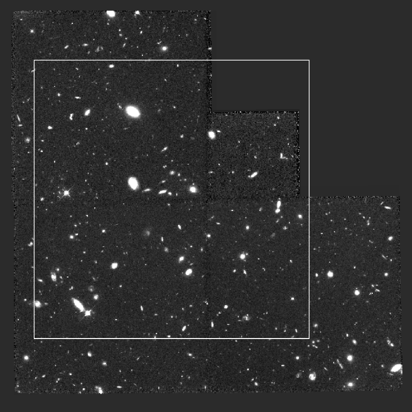
Figure 2: Field of view of CISCO $K^{\prime}$-band image relative to HST WFPC2 image.

Flux calibration to the Mauna Kea system $K$-band was carried out by observing the United Kingdon Infrared Telescope (UKIRT) faint standard stars (Hawarden et al., 2001) taken before and after the HDF-N observation.

2.2 HST WFPC2/NICMOS data

The HDF-N was observed with the HST NICMOS Camera 3 between UT 1998 June 13 and June 23 (PI:M. Dickinson; PID 7817). The complete HDF-N was mosaiced with eight sub fields in the $J_{110}$ and $H_{160}$-bands. We analyzed the calibrated data of these observations downloaded from the archival site of the Space Telescope Science Institute. Each sub field was observed through nine dithered pointings, with a net exposure of 12600s in each band, except for a few pointings that could not be used due to a guidance error of HST (Dickinson et al., 2000). We combined these data into a single mosaiced image registered to the WFPC2 image of the HDF-N, using the “drizzling” method with the $IRAF$ $DITHER$ package.

For optical data, we analyzed the public “version 2” $U_{300}$, $B_{450}$, $V_{606}$, $I_{814}$-band WFPC2 images of HDF-N produced by the STScI team. These optical and near infrared HST images were convolved with the Gaussian kernel to match the CISCO $K^{\prime}$-band point-spread function for the aperture photometry.

2.3 Source Detection and Photometry

First, we performed source detection in the CISCO $K^{\prime}$-band image using the SExtractor image analysis package (Bertin & Arnouts, 1996). A detection threshold of $\mu_{K}=22.91$ mag arcsec^-2, which corresponds to about 1.5 times pixel-to-pixel variation of the background, over 15 connected pixels was used. We adopted MAG_BEST from SExtractor as the total magnitude of each detected object. Of the sources extracted by SExtractor, objects located at the edge of WFPC2 frames and those which we identified by eye as noise peaks (mostly near the bright objects) were rejected and removed from the final catalog.

Figure 3 shows the raw number counts of the $K^{\prime}$-band frame. From this figure, we infer that the object detection is nearly complete to $K\sim$22.0. In this source detection procedure, we could not find the $K^{\prime}$-selected object which was not detected in the HST $I_{814}$, $J_{110}$, $H_{160}$-band images.

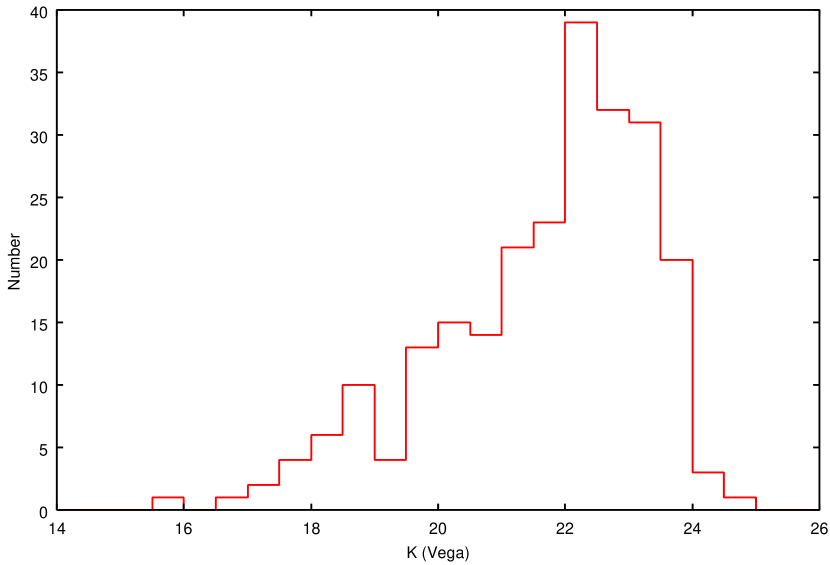
Figure 3: CISCO $K^{\prime}$-band number counts of the Hubble Deep Field North.

We cataloged the objects with $K<24.2$ (nearly all objects). To measure their color and SED, we selected the aperture size at which S/N ratio at $K^{\prime}$-band is 0.75 times that at the maximum S/N aperture. This is compromise between the highest S/N and measuring over the total lights of objects.

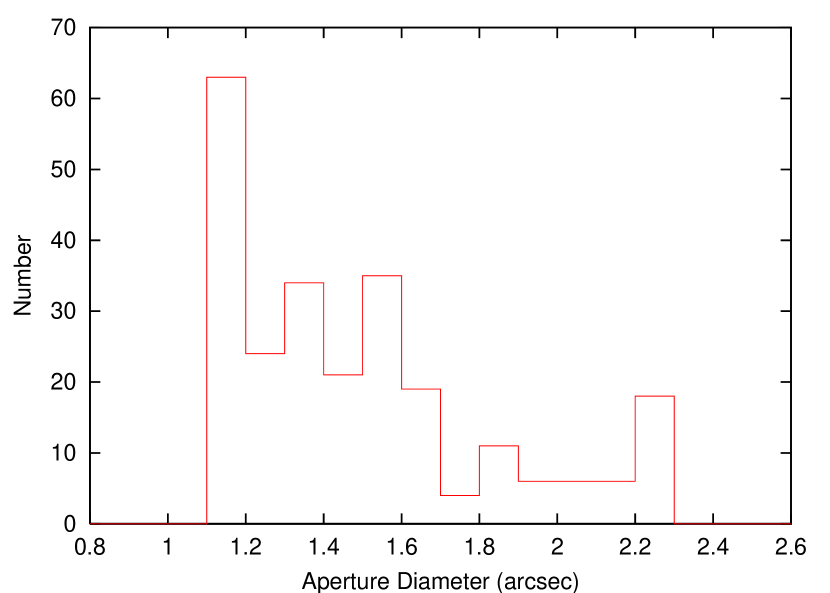
Figure 4: Adopted aperture diameter distribution for seven optical–NIR bands photometry.

The minimum aperture size is set to 1.1 arcsec diameter, which is about two times larger than the seeing size of the images, to avoid the seeing effect. The adopted aperture size was between 1.1 and 2.3 arcsec in diameter, typically $\sim$1.5 arcsec (Figure 4). With these apertures, we performed photometry for all seven $U_{300}$, $B_{450}$, $V_{606}$, $I_{814}$, $J_{110}$, $H_{160}$, $K^{\prime}$-band images. The background sky was estimated with the annulus, which has 5 arcsec inner diameter and 1 arcsec width. The aperture position for each object was fixed in order to measure the colors or broad-band SED at the same physical region of the galaxy. 247 objects were cataloged and their magnitudes were measured.

2.4 Redshift Determination and Sample Selection

Cohen et al. (2000) compiled the HDF-N galaxies with spectroscopic redshifts known by the time. We identified the corresponding objects in our $K^{\prime}$-selected catalogue by comparing the coordinates of the objects in Cohen et al.’s catalogue and ours. A few additional spectroscopic redshifts from the Team Keck Treasury Redshift Survey (Wirth et al., 2004) also could be identified in our catalogue. For 103 out of 247 objects, the spectroscopic redshifts from the literature could be used. Cohen et al.’s sample was selected mainly by the standard $R\leq 24$ mag, and limited to $z\lesssim 1.3$, except for the Lyman Break Galaxies at $z>2$ (e.g., Lowenthal et al., 1997; Dickinson, 1998). TKRS has the similar selection criterion with slightly deeper magnitude limit.

For those objects with no spectroscopic redshift, we estimated their redshifts by using the photometric redshift technique with the photometric data of the seven optical–NIR bands mentioned in the previous subsection. We computed the photometric redshifts of those objects using the public code of $hyperz$ (Bolzonella, Miralles & Pelló, 2000). The photometric redshift was calculated by $\chi^{2}$ minimization, comparing the observed magnitudes with the values expected from a set of model Spectral Energy Distribution. The free parameters involved in the fitting are the redshift, spectral type (star formation history), age, and color excess (dust extinction). We chose to use the SED model of Bruzual & Charlot synthetic library (GALAXEV; Bruzual & Charlot, 2003) and the Calzetti extinction law (Calzetti et al., 2000).

For those objects with spectroscopic redshifts, we also computed the photometric redshifts in order to test the accuracy of the photometric redshift estimate for our filter set. Figure 5 shows a comparison between the spectroscopic redshifts and photometric redshifts for those objects in our catalogue.

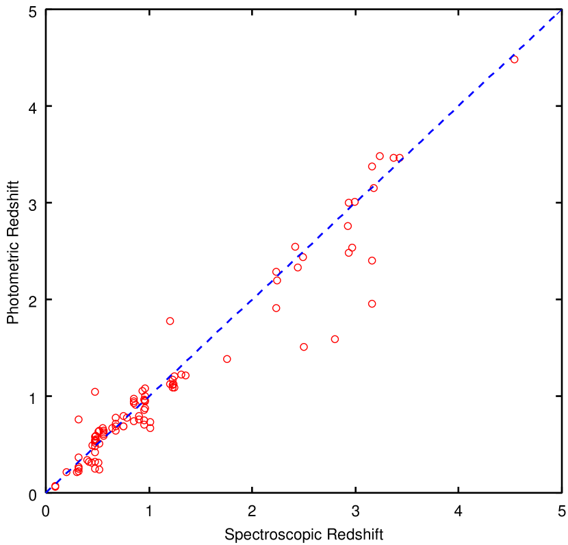
Figure 5: Comparison between the spectroscopic redshift and the photometric redshift of the $K^{\prime}$-selected galaxies with the spectroscopic redshift.

The spectroscopic and the photometric redshifts agree well within $\Delta z=0.11$ over a wide redshift range, except for several outliers.

Figure 6 shows the redshift distribution of our $K^{\prime}$-band selected galaxies. We used the spectroscopic redshifts whenever possible, and adopted the photometric redshifts for the remainder. We excluded those stars that were confirmed by spectroscopy from our sample, and did not perform any further star/galaxy discrimination for fainter objects. We use galaxies at $0.3<z<2.7$ in the following analysis.

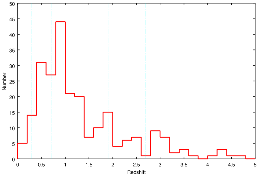
Figure 6: Redshift distribution of our $K^{\prime}$-selected galaxies. Vertical dotted-dash lines show the boundaries between the redshift bins used in the analysis.

2.5 Stellar Mass and Rest-frame Color Estimation

In addition to photometric redshift estimation, using the seven optical–NIR bands photometry, we performed the detailed SED fitting to estimate the stellar mass and rest-frame color of our sample. Like an above photometric redshift estimation, we used the GALAXEV synthetic library as the SED model. The free parameters involved in the fitting are metallicity, star formation timescale (see below), age, and color excess. The reason for varying many parameters such as metallicity in this SED fitting procedure is to investigate possible range of the stellar mass of galaxies rather than to determine each free parameter precisely. We assumed the exponentially decaying star formation rate with time (SFR $\propto e^{-t/\tau}$), and varied the characteristic timescale $\tau$ from 0.01 Gyr to 30 Gyr as a free parameter. Metallicity is changed from 0.02 solar metallicity to 2.5 solar metallicity. We assumed the Chabrier (2003)’s initial mass function (IMF) with upper and lower mass cutoffs m${}_{l}=0.1$M_⊙ and m${}_{u}=100$M_⊙, and the Calzetti extinction law. The $\chi^{2}$ value for each GALAXEV template was calculated, and the minimum $\chi^{2}$ value for each observed galaxy was found. GALAXEV code outputs the stellar mass-to-light ratio (M/L) for each template, and therefore we can estimate the stellar mass of objects from the total absolute magnitude and M/L. We calculated the (aperture) absolute $V$-band magnitude M_V, using the best-fit SED template and the redshift adopted above. The $U$-to-$K$ bands photometries allow us to measure the rest-frame $V$-band magnitude without extrapolation (use only interpolation) for galaxies at $z\lesssim 2.8$. For the objects only with photometric redshifts, we further varied redshift as a free parameter, and calculated the $\chi^{2}$ value for each GALAXEV template at various redshifts in order to investigate the effect of the photometric redshift uncertainty on the stellar mass estimate. We performed the conversion from the aperture magnitude to the total absolute magnitude by using the differences between the aperture magnitude and the MAG_BEST value at the observed $K$-band. Then the dust-extinction corrected absolute magnitude was used to calculate the stellar mass. The cosmology of $H_{0}=70$ km s^-1 Mpc^-1, $\Omega_{\rm 0}=0.3$, $\Omega_{\Lambda}=0.7$ is assumed.

As well as absolute magnitude, the rest-frame color can be estimated from the best-fit SED template. For analysis, we use the rest $U-V$ color, which is sensitive to the existence/absence of the largest features in the galaxy continuum spectra at near-UV to optical wavelengths, namely, a 4000 Å  break or the Balmer discontinuity. Since these features are sensitive to the average age of stars especially at relatively young stage, we can infer the evolution of the average age of their stars even at the region where the photometric uncertainty is relatively large. The rest-frame $U-V$ color can be estimated without extrapolation for objects at $z\lesssim 2.8$.

2.6 Morphological Classification

We performed a quantitative morphological classification for the $K^{\prime}$-selected galaxies using the HST WFPC2/NICMOS images, as described by Kajisawa & Yamada (2001). The classification method used is based on the central concentration index, $C$, and the asymmetry index, $A$ (Abraham et al., 1996). The bands used for the classification were selected so that the classification was made on the rest-frame $B$ to $V$-band image for each object ($I_{814}$-band for $z<1.0$, $J_{110}$-band for $1.0<z<2.0$, $H_{160}$-band for $z>2.0$), where various morphological studies of local galaxies have been done. Since the $C$ and $A$ indices depend on the brightness of the object, even if the intrinsic light profiles were identical, we evaluated the morphology by comparing the indices of the observed galaxy with those of a set of simulated artificial ones that have similar photometric parameters as each observed galaxy. The detail processes of the classification are described in Kajisawa & Yamada (2001).
Although some scatter exists, our quantitative $C$/$A$ classification is confirmed to correlate well with an eyeball classification by van den Bergh, Cohen, Hogg, & Blandford (2000) (Kajisawa & Yamada, 2001, Figure 8). The number of galaxies which are classified into each morphological category is 40 in bulge-dominated, 23 in intermediate, 92 in disk-dominated, 65 in irregular, respectively. The other 20 objects were cannot be classified because of their faintness.

We prefer to use a quantitative morphological classification, because it is not only more objective, but can also take into account the effect of the magnitude/surface brightness bias for classification.

3 Results

Using the very deep $U$-to-$K$ band images of the Hubble Deep Field North, we can estimate the rest-frame optical properties of galaxies to $z\sim 3$, and investigate the distribution of the stellar mass, $U-V$ color, morphology.

3.1 Stellar Mass Distribution

Figure 7 shows our estimate of the stellar mass of the sample as a function of redshift. Error bars indicate the range of 90% confidence level, which is estimated from the $\chi^{2}$ value at each position in the parameter space in the SED fitting. Circles show the objects with spectroscopic redshifts and squares represent the phot-z sample. For the phot-z sample, we took account of the uncertainty of the photometric redshift in the error estimate.

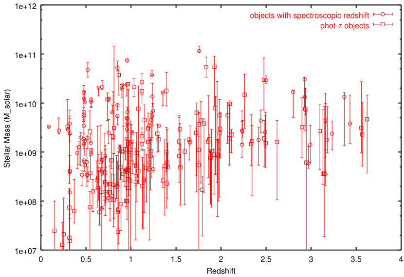
Figure 7: Stellar mass distribution of our $K^{\prime}$-selected sample of galaxies in the HDF-N as a function of redshift. Circles show objects with spectroscopic redshifts and squares represent the phot-z sample. Error bars show the range of 90% confidence level.

Because our sample is limited to $K<24.2$, only the more massive galaxies tend to be selected at the higher redshift. While we can sample galaxies to the stellar mass of $\sim 1\times 10^{8}$M_⊙ at $z\sim 1$, only galaxies with the stellar mass larger than $\sim 1\times 10^{9}$M_⊙ can be detected at $z\sim 2$. Less massive, higher redshift galaxies have fainter apparent magnitude, and therefore the constraint on the stellar mass of the galaxies tends to be weak. Furthermore, the photometries only at shorter rest-frame wavelength can be used for galaxies at higher redshift, which weakens the constraint on the stellar mass. For example, the typical 1$\sigma$ error of the mass estimate for the galaxies with stellar mass of $10^{9}-10^{10}$M_⊙ is $\sim 0.2$ dex at $z\sim 1$, and becomes $\sim 0.4$ dex at $z\sim 2$. Dickinson, Papovich, Ferguson, & Budavári (2003) estimated the stellar mass of H₁₆₀-selected galaxies in the HDF-N, using the HST WFPC2/NICMOS images and the ground-based $K$-band data with IRIM on the KPNO 4 m. Our result about the stellar mass distribution is similar with that in Dickinson et al., although the selection and the field of view are slightly different. Our stellar mass estimate with Chabrier (2003)’s IMF is about 1.8 times smaller systematically than that with Salpeter IMF, which is adopted in Dickinson, Papovich, Ferguson, & Budavári (2003).

In Figure 7, it is seen that there is few galaxies with the stellar mass larger than 1 $\times 10^{11}$ M_⊙. With small corresponding volume of the HDF-N, the expected number of galaxies with M${}_{stellar}>1\times 10^{11}$ M_⊙ is about one at $z\lesssim 1$, which is calculated from the results of 2MASS and 2df survey for local galaxies (Cole et al., 2001) assuming no evolution. At $1<z<3$, the expected number of these galaxies becomes about nine, while we detected only one galaxy with M${}_{stellar}>1\times 10^{11}$ M_⊙ in our sample. The number density of these massive galaxies seems to decrease at $z\gtrsim 1$ in the HDF-N, but the significance of such small number statistics may be relatively low, considering the field-to-field variance due to the clustering of galaxies. To investigate the number density, color, and morphology distribution of these massive galaxies with a stellar mass larger than $10^{11}$ M_⊙, the larger-volume survey is needed.

3.2 Rest $U-V$ Color vs Stellar Mass

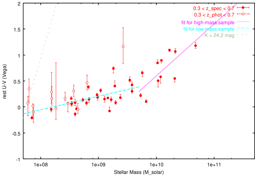
Figure 8: rest frame $U-V$ color distribution of galaxies at $0.3<z<0.7$ as a function of stellar mass. Solid circles represent the objects with spectroscopic redshifts, and open circles show the phot-z sample. Error bars represent the range of 90% confidence level. Short-dashed line shows the corresponding detection limit estimated from the various GALAXEV models with $K=24.2$. Dotted line and long-dashed line represent the fitting results for the high-mass sample and the low-mass sample.

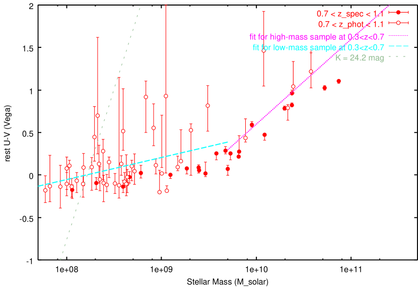
Figure 9: Same as Figure 8, but for galaxies at $0.7<z<1.1$. For comparison, the fitting results for the low-mass sample and high-mass sample at $0.3<z<0.7$ are showed.

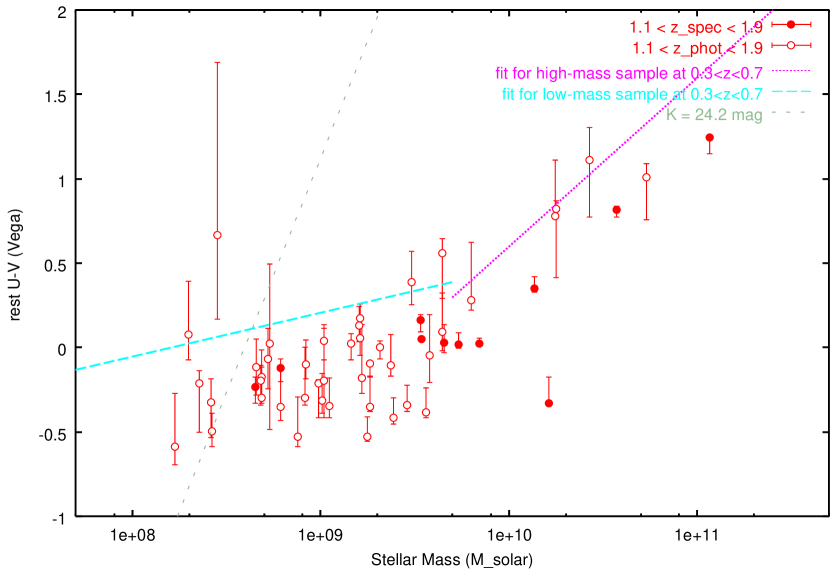
Figure 10: Same as Figure 9, but for galaxies at $1.1<z<1.9$.

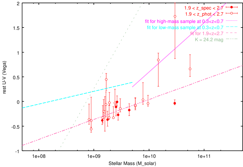
Figure 11: Same as Figure 9, but for galaxies at $1.9<z<2.7$.

Figure 8-11 show the rest $U-V$ color distribution of our $K^{\prime}$-selected galaxies in the HDF-N as a function of stellar mass for each redshift bin. For local galaxies, the $U-V$ color range is $\sim 1.2$-1.5 for E and S0 galaxies, $\sim 0.7$-1.1 for Sa-Sb galaxies, and $\sim 0$-0.6 for Sc-Irr galaxies, respectively.
The range of each redshift bin is selected such that the photometric redshift uncertainty does not affect strongly the membership in each redshift bin. In figure 6, which shows the redshift distribution of our sample, vertical dotted-dash lines represent the boundary of each redshift bin. In our assumed $H_{0}$ = 70 km s^-1 Mpc^-1, $\Omega_{\rm 0}=0.3$, $\Omega_{\Lambda}=0.7$ cosmology, the corresponding co-moving volume of each redshift bin is 1332 Mpc³ for $0.3<z<0.7$ bin, 2720 Mpc³ for $0.7<z<1.1$, 7885 Mpc³ for $1.1<z<1.9$ bin, 8948 Mpc³ for $1.9<z<2.7$, respectively. The number of objects in each redshift bin is 53 in $0.3<z<0.7$ bin, 70 in $0.7<z<1.1$ bin, 54 in $1.1<z<1.9$ bin, 28 in $1.9<z<2.7$, respectively. Solid symbols represent the objects with spectroscopic redshifts and open symbols show those with photometric redshifts. Error bars in Figure 8-11 show the $U-V$ range of 90% confidence level for the SED fitting. For the phot-z sample, the uncertainty of photometric redshift is taken into account in the confidence level.
The detection limit corresponding to $K=24.2$ was estimated from the GALAXEV models. Using the GALAXEV models with various age and star formation timescale $\tau$ (solar metallicity and no dust extinction are assumed), we calculated the stellar masses and the rest $U-V$ colors for the models with $K=24.2$ and the corresponding redshift range. We simply performed the linear fit for these calculated masses and colors, and the result is showed as the short-dashed line in Figure 8-11.

In Figure 8 and 9, it is seen that there is few galaxies with relatively blue color (e.g., $U-V<0.3$) at M${}_{stellar}>1\times 10^{10}$M_⊙. On the other hand, at M${}_{stellar}\lesssim 5\times 10^{9}$M_⊙, the number of objects with red color (e.g., $U-V>0.6$) is much smaller than the bluer galaxies. At M${}_{stellar}\sim 5\times 10^{9}$M_⊙, the transition of rest $U-V$ color distribution seems to occur. In Figure 10, the similar transition of the color is also seen at $1.1<z<1.9$. At M${}_{stellar}\lesssim 5\times 10^{9}$M_⊙, most galaxies have $U-V\lesssim 0$, while redder galaxies dominate at M${}_{stellar}\gtrsim 5\times 10^{9}$M_⊙. At $1.9<z<2.7$ (Figure 11), the number of red (e.g., $U-V\gtrsim 0.5$) or massive (e.g., $\gtrsim 10^{10}$M_⊙) galaxies is very small, and it is uncertain whether the trend seen at lower redshifts exists or not.

To contrast the transition of the rest-frame color, in Figure 12, we show the $U-V$ color histogram for galaxies with M${}_{stellar}<5\times 10^{9}$M_⊙ and M${}_{stellar}>5\times 10^{9}$M_⊙, respectively.

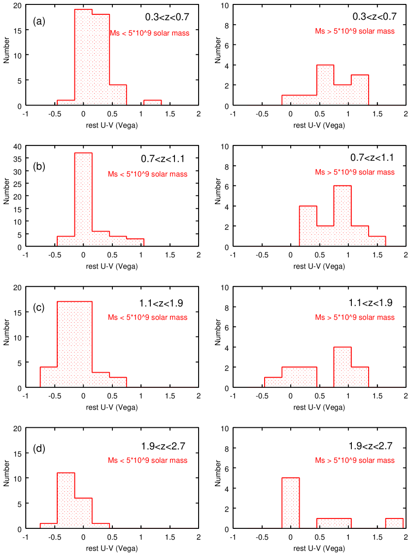
Figure 12: Rest $U-V$ color distribution of galaxies when the sample is divided into two populations at 5$\times 10^{9}$M_⊙. left:for galaxies with M${}_{stellar}<5\times 10^{9}$M_⊙, right:for galaxies with M${}_{stellar}>5\times 10^{9}$M_⊙. Each row corresponds to each redshift bin. (a):$0.3<z<0.7$, (b):$0.7<z<1.1$, (c):$1.1<z<1.9$, (d):$1.9<z<2.7$.

In the Figure 12a and 12b, the differences of the $U-V$ distributions of these low- and high-mass samples are seen. While the rest $U-V$ color distribution of the low-mass sample shows the peak at $U-V\sim$0-0.3, the high-mass sample has redder $U-V$ distribution. In figure 12c and 12d, we show the same comparison of rest $U-V$ color distribution for galaxies at $1.1<z<1.9$ and $1.9<z<2.7$. At $1.1<z<1.9$, the similar trend with that at $z<1.1$ is clearly seen. On the other hand, this trend is less secure at $1.9<z<2.7$.

In Figure 8 and 9, the low- and high-mass samples seem to have different dependences of rest $U-V$ color on their stellar mass. While the rest $U-V$ color of the high-mass galaxies is strongly correlated with the stellar mass (more massive galaxies have redder color), the correlation between the $U-V$ color and stellar mass seems to be very weak in the low-mass population. To quantify this trend, we performed the linear fit in the rest $U-V$ vs $\log{M_{stellar}}$ plane for the high-mass and the low-mass sample, respectively at each redshift bin. The result is summarized in Table 1. The estimated value of slope is 0.260$\pm$0.096 for the low-mass population, 1.002$\pm$0.269 for the high-mass population at $0.3<z<0.7$. At $0.7<z<1.1$, the slope for the low-mass sample is 0.152$\pm$0.095, and that for the high-mass sample is 0.801$\pm$ 0.196. These results confirm that the rest $U-V$ color of galaxies with M${}_{stellar}<5\times 10^{9}$M_⊙ is only weakly correlated (or not correlated) with stellar mass. At $1.1<z<1.9$, the fitted slope is 0.049$\pm$0.119 for the low-mass sample, 0.980$\pm$0.279 for the high-mass sample, which shows that the similar trend with that at $z\lesssim 1$ is maintained at this redshift range. Results for galaxies at $1.9<z<2.8$ is 0.450$\pm$0.546 for the low-mass sample, 0.425$\pm$0.437 for the high-mass one. We cannot find the difference of the $U-V$ color dependence on stellar mass between the samples divided at 5$\times 10^{9}$M_⊙ at this redshift range, as can be seen from Figure 11. Instead, over the mass range of 1$\times 10^{9}$–1$\times 10^{10}$M_⊙, the trend that galaxies with higher stellar mass have redder $U-V$ color is seen. We performed the same linear fitting as above for all (low-mass and high-mass samples) galaxies in $1.9<z<2.7$ bin, and showed the result in Figure 11. The estimated slope is 0.405$\pm$0.162.

It should be noted that our $K^{\prime}$-selected sample does not strictly correspond to the stellar mass-selected one. If we consider the same stellar mass galaxies at the same redshift, galaxies with the redder color tend to have the lower $K$-band magnitude, because they are dominated by older stellar population or are highly dust-extincted, and have higher mass-to-light ratio. Therefore, near the lower limit of stellar mass of the sample (near the detection limit of our $K^{\prime}$-band observation), there is the bias against the detection of redder galaxies in each redshift bin. At least $z\lesssim 2$, however, the rest $U-V$ distribution seen in Figure 8-10 become rather blue and the stellar mass dependence of the $U-V$ color becomes weak at the stellar mass of $\sim 5\times 10^{9}$M_⊙, which corresponds to the value much higher than the detection limit of our observation, and therefore this bias does not seem to influence significantly our results about the color distribution and their dependence on stellar mass.
At $1.9<z<2.7$, where the $K$-band detection limit corresponds to $\sim 1\times 10^{9}$M_⊙, the bias against the redder galaxies may affect the slope of the correlation between the stellar mass and the $U-V$ color (see short-dashed line in Figure 11). As seen in Figure 11, however, there is the trend that the $U-V$ color of the bluest galaxies at each stellar mass becomes bluer as the stellar mass decreases, which cannot be explained by this bias.
Furthermore, in order to investigate the stellar mass value where the change of the mass dependence of the rest $U-V$ color occurs, we retried the linear fit in the rest $U-V$ vs $\log{M_{stellar}}$ plane, varying the boundary mass between the high- and low-mass samples as a free parameter in each redshift bin. The best fit boundary stellar mass is 6.76${}^{+5.24}_{-3.29}\times 10^{9}$M_⊙ at $0.3<z<0.7$, 7.08${}^{+12.9}_{-5.26}\times 10^{9}$M_⊙ at $0.7<z<1.1$, 3.63${}^{+13.0}_{-2.19}\times 10^{9}$M_⊙ at $1.1<z<1.9$, respectively. We could not find the significant evolution of the stellar mass where the mass dependence of the rest $U-V$ color changes, although we could not constrain strongly this stellar mass in each redshift bin.

To estimate the degree of the evolution of the $U-V$ color distribution as a function of stellar mass, in Figure 9-11, we compared the $U-V$ distribution of galaxies at $0.7<z<1.1$, $1.1<z<1.9$, $1.9<z<2.7$, respectively, with the fitting result for those at $0.3<z<0.7$. From these figures, it is seen that at M${}_{stellar}<5\times 10^{9}$M_⊙, the rest $U-V$ distribution become gradually bluer with redshift. At $0.3<z<0.7$, the envelope of galaxies with the bluest $U-V$ color lies at $U-V\sim-0.1$. On the other hand, the bluest galaxies at $1.1<z<1.9$ have $U-V\sim-0.5$. For simplicity, we ignored the small slope in the $U-V$ vs stellar mass plane for the low-mass sample and calculated the average $U-V$ value of galaxies with M${}_{stellar}<5\times 10^{9}$M_⊙ at each redshift bin. The result is 0.153$\pm$0.173 at $0.3<z<0.7$, 0.019$\pm$0.142 at $0.7<z<1.1$, -0.081$\pm$0.157 at $1.1<z<1.9$, -0.241$\pm$0.186 at $1.9<z<2.7$.
On the contrary, the relation between the stellar mass and rest $U-V$ color of galaxies with M${}_{stellar}>5\times 10^{9}$M_⊙ does not seem to change significantly at $z\lesssim 2$. In fact, the rest $U-V$ distribution of the high-mass sample at $0.7<z<1.1$ and $1.1<z<1.9$ corresponds well to the fit for the high-mass galaxies at $0.3<z<0.7$, in Figure 9 and 10. We performed the fitting for the high-mass sample at $0.7<z<1.1$ and $1.1<z<1.9$, assuming the same slope as that at $0.3<z<0.7$, and compared the resultant intercept value with that at $0.3<z<0.7$. The difference of intercept is -0.115$\pm$0.274 at $0.7<z<1.1$, -0.224$\pm$0.362 at $1.1<z<1.9$, respectively, which shows the differences are less significant. At $1.9<z<2.7$, the number of galaxies with M${}_{stellar}>1\times 10^{10}$M_⊙ is very small, and the relation between the stellar mass and the rest $U-V$ seems to disappear. These results about the degree of the evolution of the rest $U-V$ color are summarized in Table 2.

The results obtained in this section are about the relation between the stellar mass and the rest-frame $U-V$ color of galaxies. Since both the stellar mass and the rest $U-V$ were calculated from the SED fitting with the population synthesis model, there can be possibility that some biases about the SED model work on the results and produce the artifacts. To check this, we estimated the rest $U-V$ color without the SED fitting procedure, using the direct linear interpolation from the observed photometries. Figure 13 shows the comparison between the rest $U-V$ colors estimated by the SED fitting with GALAXEV model and the linear interpolation. Although the estimation with SED fitting tend to over/under-estimate the rest $U-V$ color at very blue/red region, the correspondence between these two estimations is good, and the results obtained above do not change if we use the $U-V$ value calculated from the linear interpolation.

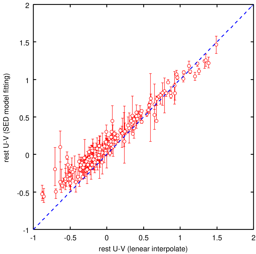
Figure 13: Comparison between the rest-frame $U-V$ colors estimated by different procedures(linear interpolation vs SED fitting with population synthesis model). Error bars represent the range of 90% confidence level.

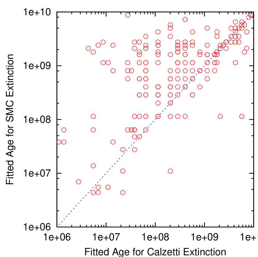
Figure 14: Comparison between the fitted ages estimated by the SED fitting with different extinction curves(Calzetti law vs SMC like extinction)

Fontana et al. (2003) pointed out that the SED fitting with the Calzetti’s extinction law yields lower fitted age than that with the Small Magellanic Cloud (SMC) like extinction curve, and that the stellar mass estimates with Calzetti law are slightly smaller. In order to check the uncertainty due to the differences of adopted extinction curves, we performed the SED fitting with SMC extinction

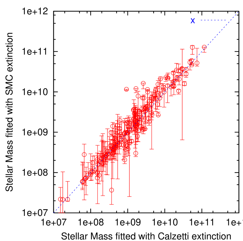
Figure 15: Comparison between the stellar masses estimated by the SED fitting with different extinction curves(Calzetti law vs SMC like extinction). Error bars represent the range of 90% confidence level.

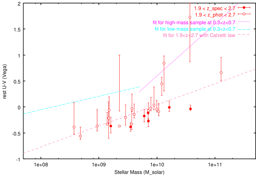
Figure 16: same as Figure 11, except that the SMC extinction curve is used in the SED fitting for the stellar mass estimation.

law (Pei, 1992), where other factors are not changed from the fitting with Calzetti law. Figure 14 shows the comparison of the fitted ages estimated with different extinction laws. As pointed out by Fontana et al. (2003), the ages estimated with SMC extinction clearly tend to have higher value than that with Calzetti law. We calculated the ratio of the stellar mass estimated with SMC extinction relative to that with Calzetti law, and found that the average of the ratio of estimated stellar masses is 0.99$\pm 0.05$. As showed in Figure 15, the stellar masses estimated from the fitting with different extinction laws seem to agree well with a few exceptions. Since the fit with SMC extinction yields higher age, estimated mass-to-luminosity ratios tend to be higher. But the degree of attenuation by dust tends to be smaller value in the fit with SMC extinction, and the estimated dust-corrected absolute magnitudes are fainter than that with Calzetti law. Because these effects tend to be canceled out, the differences in the stellar mass become smaller, especially in the case that the photometries at the long-ward wavelength constrains the rest-frame NIR flux strongly. Most of the outliers seen in Figure 15 are galaxies in the $1.9<z<2.7$ bin. We recalculated the ratio of the stellar masses of galaxies at $1.9<z<2.7$ estimated with different extinction laws, and the result is 1.41$\pm 0.17$. For these galaxies, whose observed $K$-band photometries reach only the rest-frame $V$ to $R$-band, there seems to be the trend indicated by Fontana et al. (2003) that the SED fitting with SMC extinction yields slightly larger stellar mass. For reference, we show the rest $U-V$ color distribution of galaxies at $1.9<z<2.7$ as a function of the stellar mass estimated with the SMC extinction in Figure 16. Overall trend is not changed.

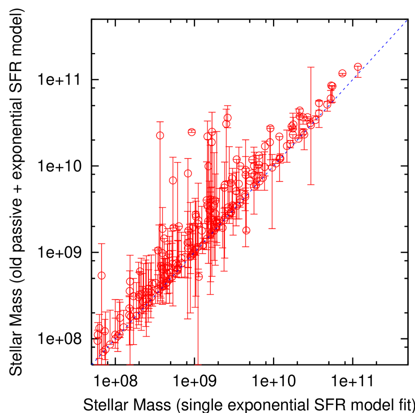
Figure 17: Comparison between the stellar masses estimated by the SED fitting with different star formation history models (single exponentially decaying SFR model vs old passive population $+$ exponential SFR model). Error bars show the range of 90% confidence level.

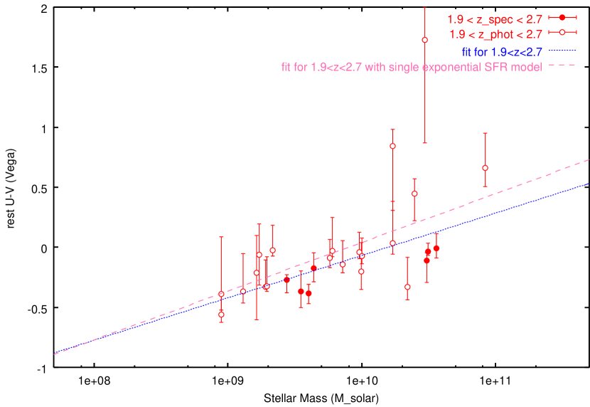
Figure 18: same as Figure 11, except that the old passive population $+$ exponential SFR model is used in the SED fitting for the stellar mass estimation.

Although we assumed simple exponentially decaying star formation rate model (characteristic timescale $\tau$ is free parameter) in the SED fitting procedure as mentioned above, we also tried to use two-component star formation history model, exponentially decaying SFR $+$ old passive-evolving population, following Papovich, Dickinson, & Ferguson (2001), in order to estimate the upper limit of the stellar mass of our sample. For the old population, we chose the single 0.01 Gyr burst model (after the burst, it evolves passively) and fix its age to the age of the Universe at the observed redshifts (formation redshift is infinity). Maximum age for the old passive population yields maximum mass-to-light ratio, and is suitable for the estimate of the upper limit mass. The relative flux ratio between exponential SFR model and old population is added as a free parameter to the SED fitting. The result is showed in Figure 17. The distribution of the best-fit stellar mass estimated with old population $+$ exponential SFR model is systematically higher than that with single exponentially decaying SFR model. The average of the ratio of those estimated with different star formation history models is 1.26$\pm 0.05$. The average ratio of the 68% upper mass limits from the two-component model relative to the best-fit stellar masses from single exponential SFR model is $2.30\pm 0.60$. Again, most of outliers in Figure 17 are galaxies in the $1.9<z<2.7$ bin. At $z\lesssim 2$, if we use the best-fit stellar mass estimated with two-component star formation history model, the overall trend about the distribution of $U-V$ color and the stellar mass is not changed. At $1.9<z<2.7$, the average ratio of the best-fit stellar masses estimated with different star formation history models becomes $1.54\pm 0.21$, and those of the 68% upper mass limits is 6.84$\pm 1.31$. For these galaxies, their faintness and relatively poor rest-frame wavelength coverage cause large uncertainty. As seen in Figure 18, however, the trend that galaxies with the higher stellar mass have the redder rest $U-V$ color is still seen, even if we use the stellar mass estimated with old population $+$ exponential SFR model. The slope of the correlation between the $U-V$ color and the stellar mass becomes $0.391\pm 0.196$.

Furthermore, in order to check the effect of our adopted aperture size (section 2.3, Figure 4), we performed the fixed aperture photometry with 1.2, 2.4, 4.0 arcsec diameter aperture, and calculated the rest $U-V$ color with the same way for

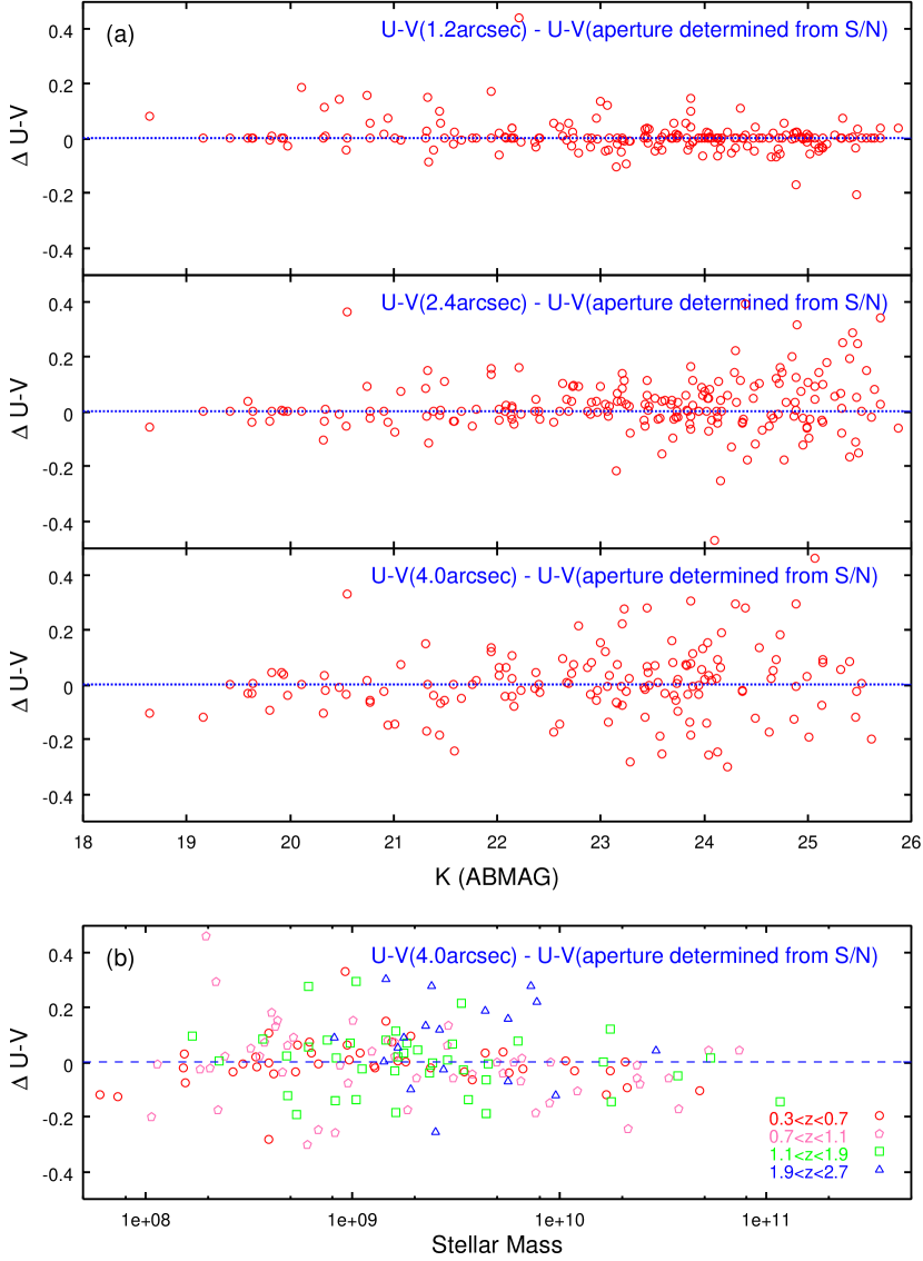
Figure 19: Differences between the rest $U-V$ colors with the apertures determined from S/N ratio and those with fixed apertures. (a): differences of $U-V$ as a function of $K$-band magnitude. top: for 1.2 arcsec diameter aperture. middle: for 2.4 arcsec diameter aperture. bottom: for 4.0 arcsec diameter aperture. (b): differences of $U-V$ as a function of stellar mass for 4.0 arcsec diameter aperture. Each symbol represents each redshift bin.

each aperture. The differences between the $U-V$ colors with our adopted aperture and those with fixed apertures are showed in Figure 19 as a function of $K$-band magnitude and stellar mass. From the Figure 19(a), it is seen that for some bright galaxies, rest $U-V$ colors become bluer as the aperture size increases. However the differences from the originally adopted aperture are at most $\sim 0.2$ mag even for a very large 4.0 arcsec diameter aperture. Further, in Figure 19(b), which show the aperture effects as a function of stellar mass, no systematic effect is seen.
The aperture effect cannot change our results about $U-V$ color distribution of galaxies as a function of stellar mass.

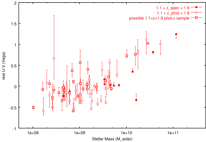
Figure 20: Same as Figure 10 except that the “possible” $1.1<z<1.9$ galaxies whose 90% confidence ranges of photometric redshifts overlap the bin range are also plotted.

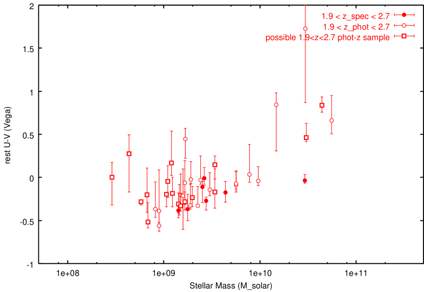
Figure 21: same as Figure 20, but for $1.9<z<2.7$.

Since our photometric redshift estimate seems to be relatively uncertain at $z\gtrsim 1.5$ (Figure 5), we checked the effects of photometric redshift uncertainty on the membership of the high-redshift bins. To do this, we picked up the objects without the spectroscopic redshift for which the best-fit photometric redshifts are not included in the considering redshift bin but the redshift ranges of their 90% confidence level in the SED fitting overlap the redshift bin as “possible sample”. Then we restricted their redshift within the considering redshift bin and evaluated the allowable ranges and the minimum $\chi^{2}$ values of the stellar mass and the rest $U-V$ color. The results for $1.1<z<1.9$ bin and $1.9<z<2.7$ bin are showed in Figure 20 and 21. In these figures, “possible sample” does not affect the distribution of galaxies in the stellar mass vs rest $U-V$ plane significantly. Some objects whose best-fit photometric redshift is included in the redshift bin could similarly escape from the bin, but such uncertainty about the photometric redshift does not seem to change the results obtained above.

3.3 Morphology vs Stellar Mass

In the previous subsection, we found that from the behavior of the rest-frame $U-V$ color distribution, galaxies at $z\lesssim 2$ can be divided into two populations at around the stellar mass of $\sim 5\times 10^{9}$M_⊙. In this section, we examine the relationship between these populations divided by stellar mass and their morphology.

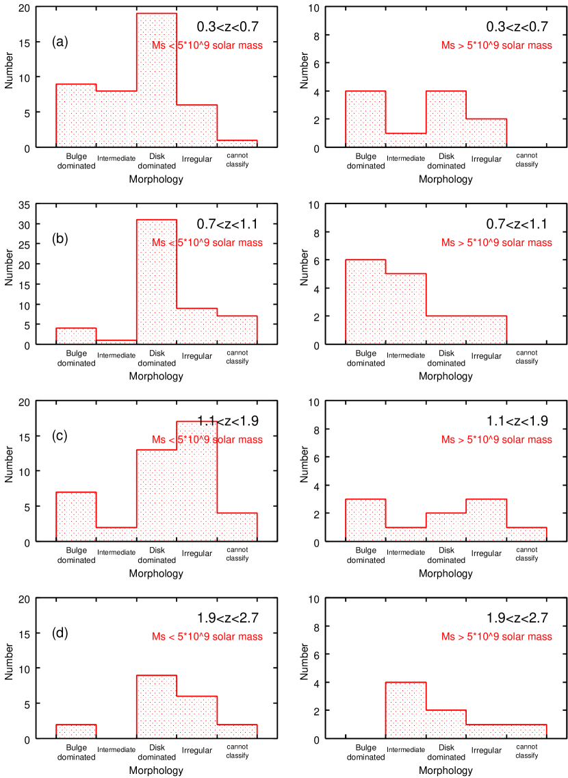
Figure 22: Morphological distribution of our $K^{\prime}$-selected galaxies at $0.3<z<2.7$ in the HDF-N. left: for galaxies with with M${}_{stellar}<5\times 10^{9}$M_⊙. right: for galaxies with M${}_{stellar}>5\times 10^{9}$M_⊙. Each row corresponds to each redshift bin. (a):$0.3<z<0.7$, (b):$0.7<z<1.1$, (c):$1.1<z<1.9$, (d):$1.9<z<2.7$.

In Figure 22, we show the morphological distribution of the $K^{\prime}$-selected galaxies in the HDF-N at each redshift bin with M${}_{stellar}<5\times 10^{9}$M_⊙ and M${}_{stellar}>5\times 10^{9}$M_⊙ separately. From Figure 22a and 22b, it is seen that disk galaxies dominate the low-mass population at $z\lesssim 1$. In the high-mass sample, the various morphological types have similar fraction, and the fraction of bulge-dominated galaxies seems to be higher than that in the low-mass sample, although the small number of the high-mass sample causes large uncertainty. At $1.1<z<1.9$, the number of irregular galaxies increases and becomes similar with that of disk-dominated galaxies in the low-mass sample, while the bulge-dominated galaxies and irregular galaxies seem to have similar number in the high-mass sample. In our morphological classification, since the galaxies classified into irregular category show the significantly high asymmetry index relative to those of artificial galaxies with similarly faint brightness, it is not the case that fainter galaxies tends to be classified into the irregular category because of the noise effect. At $1.9<z<2.7$, the similar morphological fraction with that at $1.1<z<1.9$ is seen.

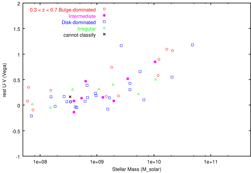
Figure 23: $U-V$ distribution of galaxies with each morphology at $0.3<z<0.7$ as a function of stellar mass. Each symbol represents morphological type. Circles:bulge-dominated galaxies, Asterisks:intermediate, Squares:disk-dominated galaxies, Triangles:irregular galaxies, crosses:galaxies cannot be classified because of their faintness.

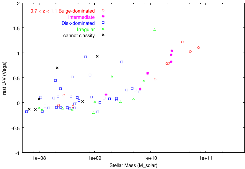
Figure 24: Same as Figure 23, but for galaxies at $0.7<z<1.1$.

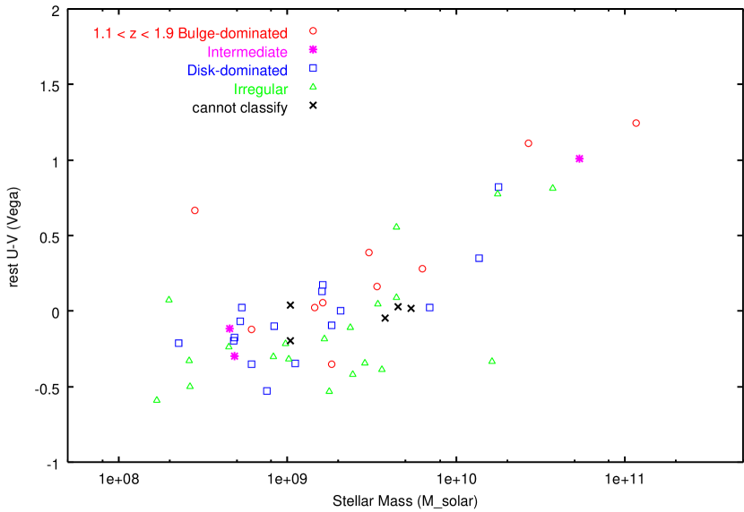
Figure 25: Same as Figure 23, but for galaxies at $1.1<z<1.9$.

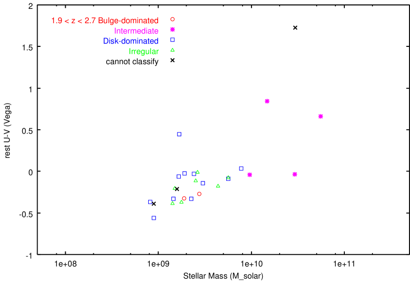
Figure 26: Same as Figure 23, but for galaxies at $1.9<z<2.7$.

Figure 23-26 show the rest $U-V$ color distribution of galaxies with each morphological type as a function of stellar mass. We also see here the trend that disk-dominated galaxies (and irregulars at $z\gtrsim 1$) dominate the low-mass population, and that in the high-mass population, the fraction of galaxies with earlier-type morphology (bulge-dominated and intermediate) is larger than that in the low-mass sample at $0.3\lesssim z\lesssim 2.7$. Furthermore, in the stellar mass range of M${}_{stellar}\gtrsim 5\times 10^{9}$M_⊙, there seems to be the trend that the more massive galaxies have the earlier morphology.

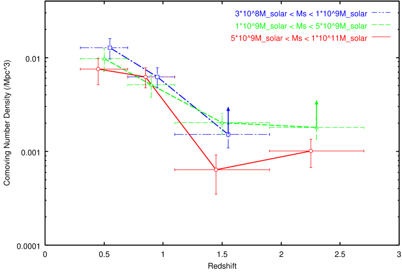
Figure 27: Comoving number density of galaxies in each stellar mass range as a function of redshift. Each symbol represents the stellar mass range. Error bars are based on the square root of the observed number. Arrows show that these bins are near the detection limit and should be regarded as lower limit considering the incompleteness.

In Kajisawa & Yamada (2001), we investigated the morphological number density evolution of galaxies with M${}_{V}<-20$ at $z<2.0$ in the HDF-N, and found that the number density and morphological fraction of bulge-dominated galaxies decreases at $z>1$. Stanford et al. (2004) also studied the properties of HST/NICMOS-selected early-type galaxies in the HDF-N and found that the number density of morphologically selected early-type galaxies decreases at $z\gtrsim 1.4$. On the other hand, in Figure 22, each morphological fraction in the high and the low-mass samples does not show significant change at $0.3\lesssim z\lesssim 2.7$, except that the fraction of irregular galaxies increases at $z\gtrsim 1$. In order to consider the consistency between these results, in Figure 27, we show the number density evolution of each range of stellar mass. In the figure, it is seen that the number density of the high-mass galaxies decreases rapidly at $z>1$ relative to that of the low-mass sample in the HDF-N, although the uncertainty is relatively large. It is noted that since we did not correct for the incompleteness in this figure, the data of $1.1<z<1.9$ bin for the stellar mass range of $3\times 10^{8}$-$1\times 10^{9}$M_⊙ and $1.9<z<2.7$ bin for $1\times 10^{9}$-$5\times 10^{9}$M_⊙, which are near the detection limit of our sample, should be considered as lower limit value (arrows in the figure), and the difference of the number density decreases at $z>1$ between for galaxies with M${}_{stellar}>5\times 10^{9}$M_⊙ and with M${}_{stellar}<5\times 10^{9}$M_⊙ could become larger than that seen in Figure 27. Since the fraction of early-type morphology is larger in the high-mass sample as mentioned above, in the overall mass range, the fraction of early-type is expected to decrease at $z>1$, and our result about the morphological distribution as a function of stellar mass is consistent with the result in Kajisawa & Yamada (2001).

4 Discussion

In the previous section, using the HST WFPC2/NICMOS archival data and very deep Subaru/CISCO $K^{\prime}$-band image of the Hubble Deep Field North, we investigated the distribution of the rest $U-V$ and morphology as a function of stellar mass back to $z\sim 3$. In the estimate of the stellar mass of each galaxy, even if each parameter such as stellar age, star-formation timescale, or dust-extinction is not constrained so strongly, since the effects of these parameters tend to be cancelled out as discussed above (see Papovich, Dickinson, & Ferguson, 2001 for detailed discussion), we can evaluate the stellar mass with relatively high accuracy. Since the rest-frame $U-V$ color and rest-optical morphology are also measured from the observed $U$ to $K$-band images without extrapolation, our results obtained in the previous section are based on the robust quantities. We here discuss some possible scenarios about galaxy formation and evolution inferred from the obtained results. We consider the change of the mass dependence of the rest-frame color at the characteristic stellar mass first, and then discuss the evolution of the low-mass and the high-mass population, respectively.

4.1 Characteristic Stellar Mass

First, we found that over $0.3<z<2$, the rest $U-V$ dependence on the stellar mass changed at M${}_{stellar}\sim 5\times 10^{9}$M_⊙; in the high-mass region, the rest $U-V$ color of galaxies is strongly correlated with the stellar mass and the trend that the more massive galaxies have the redder $U-V$ color is seen. In the low-mass region, on the other hand, the $U-V$ color does not change so much along the stellar mass. Because the $U-V$ color is sensitive to the star formation histories, this indicates that the star formation activities of galaxies are related with their stellar mass at each epoch.
In our analysis, the stellar mass at which this change of the mass dependence of the rest-frame color occurs does not change significantly to $z\sim 2$. Since most galaxies with M${}_{stellar}\lesssim 5\times 10^{9}$M_⊙ have similarly blue $U-V$ color, which indicates active star formation, therefore the characteristic stellar mass for some mechanism which suppresses the star formation activities seems to be independent of redshift at $0.3\lesssim z\lesssim 2$.

For local galaxies, Kauffmann et al. (2003) reported the similar dependence of star formation histories on the stellar mass based on the Sloan Digital Sky Survey data. In their analysis, galaxies divide into two populations at M${}_{stellar}\sim 3\times 10^{10}$M_⊙, which is higher value than that we found for galaxies in the HDF-N. As seen from their Figure 1 (D_n4000 or H$\delta$ vs stellar mass), however, while their low-mass population spreads over the range of 1$\times 10^{8}$-5$\times 10^{9}$M_⊙, the high-mass population has the peak at a stellar mass larger than $\sim 5\times 10^{11}$M_⊙, where we detected few galaxies in the HDF-N. Therefore the high-mass population in our analysis corresponds to the transition zone in Kaffumann et al.’s analysis, and the trend that the correlation between star formation activity and the stellar mass changes at $\sim 5\times 10^{9}$M_⊙ is also seen for local galaxies in the SDSS data.

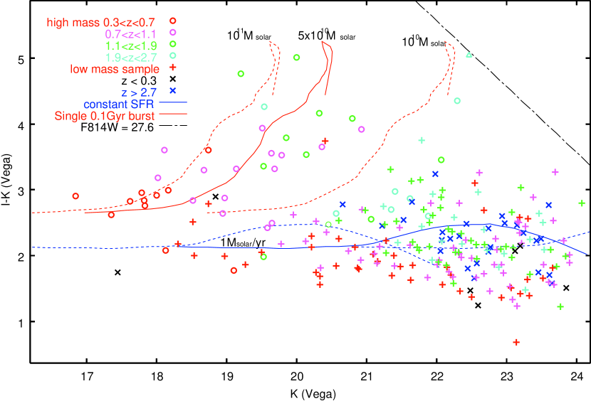
Figure 28: Observed $I_{814}-K$ vs $K$ color-magnitude diagram for our $K^{\prime}$-selected sample in the HDF-N. Circles represent galaxies with M${}_{stellar}>5\times 10^{9}$M_⊙, while crosses show galaxies with M${}_{stellar}<5\times 10^{9}$M_⊙. Color of each symbol represents its redshift. Objects without the redshift range of our analysis (i.e. objects with $z<0.3$ or $z>2.7$) are showed as X symbols (black for $z<0.3$, blue for $z>2.7$). For comparison, the 0.1 Gyr single burst models(red lines) and constant star formation rate models (blue lines) are showed as sequences of redshifts ($0.3<z<2.7$). These models assume solar metallicity and no dust extinction, and formation redshift of 3.5. For single burst model, the models with a stellar mass of 1$\times 10^{11}$M_⊙(dashed line), 5$\times 10^{10}$M_⊙(solid line), 1$\times 10^{10}$M_⊙(dashed line) are showed. For constant star formation models, the models with a star formation rate of 0.1M_⊙ yr^-1 (dashed), 1M_⊙ yr^-1 (solid), 10M_⊙ yr^-1 (dashed) are showed.

At $1.9<z<2.7$, the number of galaxies with M${}_{stellar}>1\times 10^{10}$M_⊙ in our sample becomes very small. Furthermore, our detection limit corresponds to $\sim 1\times 10^{9}$M_⊙ at this redshift range. Therefore we cannot confirm whether the change of the dependence of $U-V$ color on the stellar mass occur or not, although we found that galaxies with higher stellar mass tend to have redder rest $U-V$ color in the mass range of $\sim 1\times 10^{9}$–1$\times 10^{10}$M_⊙. Fontana et al. (2003) found that in addition to the star forming galaxies, there are a few red galaxies at $z\gtrsim 2$ in the HDF-S, and that as the stellar mass increases, the fraction of older objects seems to increase, although the biases against old/passive objects exist at low-mass region. These results suggest that the mechanism which suppresses the star formation in high-mass galaxies may work at these earlier epochs.

The difference of color distribution between the low and high-mass samples is also seen in the observed color–magnitude diagram, which is not affected by the uncertainty of redshift determination. Figure 28 shows the observed $I_{814}-K$ vs $K$ diagram for our $K^{\prime}$-selected sample in the HDF-N. The symbols represent their stellar masses: circles represent galaxies with M${}_{stellar}>5\times 10^{9}$M_⊙, and crosses show galaxies with M${}_{stellar}<5\times 10^{9}$M_⊙. Objects without the redshift range of our analysis are showed as X symbols. Color of each symbol shows its redshift. In this figure, for comparison, the 0.1Gyr single burst (thereafter passively evolving) models with a stellar mass of 1$\times 10^{10}$M_⊙, 5$\times 10^{10}$M_⊙, 1$\times 10^{11}$M_⊙ and the constant star formation models with a star formation rate of 0.1M_⊙ yr^-1, 1M_⊙ yr^-1, 10M_⊙ yr^-1 are showed as sequences of redshift between 0.3 and 2.7. The distribution of galaxies in the HDF-N in $I_{814}-K$ vs $K$ diagram can be divided into two groups: the one group is spread near the passive evolution models, the other has fainter $K$-magnitude and bluer $I_{814}-K$ color, and is spread around the constant star formation models. The gap between two groups seems to lie roughly along the single burst model with a stellar mass of 10¹⁰M_⊙. This reflects the result discussed above that the change of the rest $U-V$ color distribution at a stellar mass of $\sim 5\times 10^{9}$M_⊙ is seen at $0.3\lesssim z\lesssim 2$. The similar gap in the $I_{814}-K$ vs $K$ diagram is also seen in the Hawaii Deep Survey (Cowie, Hu, & Songaila, 1995), or 53W002 field (Yamada et al., 2001).

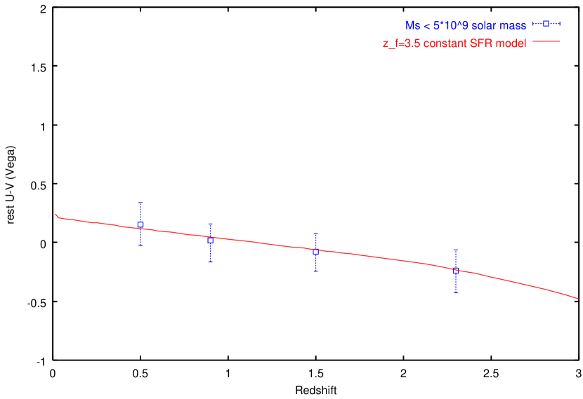
Figure 29: Rest-frame $U-V$ color of constant star formation rate model with formation redshift of 3.5 as a function of redshift. Squares represent the average $U-V$ color of galaxies with M${}_{stellar}<5\times 10^{9}$M_⊙ at each redshift bin. Errorbars show the root mean square around the average value.

4.2 The Low-mass Population

Second, we found that while the $U-V$ color of galaxies with M${}_{stellar}<5\times 10^{9}$M_⊙ is only weakly correlated with their stellar mass, the average of their $U-V$ color becomes bluer with redshift from $U-V\sim 0.2$ at $z\sim 0.5$ to $U-V\sim-0.2$ at $z\sim 2$. Their bluer color of galaxies at higher redshifts indicates that their average stellar age is younger. On the other hand, the $U-V$ color of the low-mass sample at $0.3<z<0.7$ ($U-V\sim 0.2$) indicates that active star formation still occurs in these galaxies. Since the most of the galaxies with M${}_{stellar}<5\times 10^{9}$M_⊙ have such blue $U-V$ colors at any redshifts between $z\sim 0.3$ and $z\sim 2.7$, these galaxies seem to have relatively long characteristic timescale of star formation, although in our SED fitting in section 2.5, the star formation timescale $\tau$ of each galaxy at each redshift cannot be constrained strongly.

If we consider constant SFR model, the color of $U-V\sim-0.2$ at $z\sim 2$ indicates that their stellar age is $\lesssim$1Gyr old, and their formation redshift does not seem to be much higher than the observed epoch. For example, Figure 29 shows the rest $U-V$ color of the constant star formation rate model with formation redshift of 3.5 calculated with GALAXEV code, as a function of redshift. $H_{0}$ = 70 km s^-1 Mpc^-1, $\Omega_{\rm 0}=0.3$, $\Omega_{\Lambda}=0.7$ cosmology and solar metallicity are assumed. Such a simple model can reproduce the $U-V$ color distribution of the low-mass sample at each redshift relatively well.

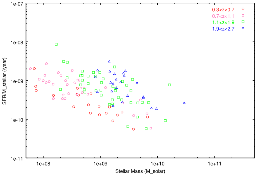
Figure 30: Estimated star formation rate relative to stellar mass of galaxies with $U-V<0.5$ as a function of stellar mass. Symbols represent corresponding redshift bins.

If we assume the continuous star formation for these low-mass galaxies as discussed above, to what extent these star formation activities can grow their stellar mass ? Since in our SED fitting procedure, where star formation time-scale $\tau$, age, and dust-extinction are free parameter, the star formation rate or star formation time-scale of each galaxy can be only very weakly constrained, here we assume simply the constant star formation rate ($\tau=\infty$) and no-extinction in order to do the rough estimation of the star formation rate of each galaxy. We derived the star formation rate of these galaxies from the observed photometry which corresponds to the rest-frame 1500-2000 Å, comparing the GALAXEV model with constant SFR, solar metallicity, Chabrier et al.’s IMF. Under these assumptions, the absolute magnitude at $\sim$1500-2000Å is insensitive to the age at larger than 0.5 Gyr old, and seems to be the good indicator of star formation rate. The results are showed as the star formation rate relative to stellar mass, namely specific star formation rate, in Figure 30. From the figure, it is seen that at the same stellar mass, the star formation rate become gradually higher as redshift increases. It is noted that at M${}_{stellar}\lesssim 10^{9}$M_⊙, galaxies at $z\gtrsim 2$ are not selected into our sample because of the detection limit of our observation. At $z\gtrsim 1$, the galaxies with a stellar mass of $\sim 1\times 10^{9}$M_⊙ form stars at the rate of 0.5–1M_⊙ yr^-1, which corresponds that the stellar mass of these galaxies would become about 1.5–2.0 times larger after 1Gyr. At $0.7<z<1.1$, the star formation rate of those with M${}_{stellar}\sim 1\times 10^{9}$M_⊙ becomes slightly smaller, and the stellar mass of these galaxies become no more than about 1.2–1.5 times larger per 1Gyr. The smaller stellar mass galaxies seem to have higher specific star formation rate. Those galaxies with M${}_{stellar}\sim 1\times 10^{8}$M_⊙ will have about twice stellar mass at 1 Gyr after if star formation rate would continue to be constant. The growth rate of stellar mass is still smaller at $0.3<z<0.7$.

On the other hand, the specific star formation rate represents the inverse of the age of the objects under the assumption of the constant SFR. We can compare these ages estimated from the star formation rate and the stellar mass with the formation epoch inferred from the rest-frame color evolution. For example, the constant SFR model with formation redshift of 3.5, which can explain the evolution of the average $U-V$ color well in Figure 29, becomes 1Gyr old at $z\sim 2.3$, 2.4Gyr at $z\sim 1.5$, 4.4Gyr at $z\sim 0.9$, and 6.6Gyr at $z\sim 0.5$, respectively. The corresponding specific star formation rate becomes from $1\times 10^{-9}$ yr^-1 at $z\sim 2.3$, to $1.5\times 10^{-10}$ yr^-1 at $z\sim 0.5$. In Figure 30, however, the specific star formation rates estimated from the rest-UV luminosity are wide-spread in each redshift bin, and the star formation rates of some galaxies seem to be inconsistent with the formation epoch inferred from the rest $U-V$ color evolution. For example, the galaxies with M${}_{stellar}\sim 1\times 10^{8}$M_⊙ at $0.7<z<1.1$ have the specific star formation rate of $\sim 1\times 10^{-9}$ yr^-1, and their formation epoch is expected to be about 1Gyr before the observed time, which corresponds to $z\sim$1-1.5. These discrepancies may be explained by the following factors which could affect our estimation of the star formation rate and the mass growth rate.
So far, several studies of Lyman break galaxies at $z\gtrsim 2$ suggested that they are shrouded in some amount of dust, typically E(B-V)$\sim 0.15$ with relatively large scatter (e.g., Steidel et al., 1999; Papovich, Dickinson, & Ferguson, 2001; Shapley et al., 2001). In fact, the best-fit E(B-V) of these low-mass blue galaxies in our sample has similar distribution with large scatter, although we can only weakly constrain the amount of the extinction of these galaxies. If we consider such an amount of dust extinction for these low-mass galaxies, the estimated star formation rates could become several times to an order of magnitude larger.
Several studies also suggested that the star formation in Lyman break galaxies is recurrent with relatively short timescale (Papovich, Dickinson, & Ferguson, 2001; Shapley et al., 2001). Glazebrook et al. (1999) also pointed out that the H$\alpha$ and UV luminosity of star forming galaxies at $z\sim 1$ indicates their star formation occurs in episodic bursts. Since most low-mass galaxies in our sample have rather blue rest $U-V$ color at any redshifts between $z\sim 0.3$ and $z\sim 2.7$ as mentioned above, the duty cycle of star formation should have relatively short timescale (e.g., $\lesssim 0.5$-1Gyr) if we assume those recurrent star formation activities. In this case, the expected stellar mass growth of these galaxies depends on the period of the duty cycle. Therefore, the formation epoch calculated from the stellar mass and the star formation rate at the observed time under the assumption of the constant SFR may not necessarily corresponds to that inferred from the color evolution.

With regard to morphological distribution, while disk-dominated galaxies dominate this low-mass population at $z\lesssim 1$, the fraction of irregular galaxies increases at $1.1<z<1.9$. The $U-V$ color distribution of irregular galaxies at $0.7<z<1.9$ is similar to, or slightly bluer than that of disk-dominated galaxies. If we assume that most of these irregular galaxies are merger origin (or interactions), these processes do not seem to change their colors. Namely, such processes may not ceases the star formation activities in these low-mass galaxies.

4.3 The High-mass Population

Third, we found that the correlation between the stellar mass and the rest $U-V$ color of galaxies with M${}_{stellar}\gtrsim 5\times 10^{9}$M_⊙ does not show significant evolution between $0.3\lesssim z\lesssim 2$. These high-mass galaxies have redder color, and earlier type morphology than the low-mass sample. For galaxies at $0.2<z<1.0$, Brinchmann & Ellis (2000) estimated the stellar mass of galaxies with spectroscopic redshift, using the Optical and NIR photometries from the Canada France Redshift Survey data, and investigated the relation between the stellar mass and the specific star formation rate. At the range of stellar mass of $9.5\lesssim$logM${}_{stellar}\lesssim 12.0$, which corresponds to their sample selection of $17.5<I<22.5$, they found that the more massive galaxies tend to have the smaller specific star formation rate and that these correlations evolve only slightly to more active star-forming between $z\sim 0.2$ and $z\sim 1.0$ (their Figure 3). Since the specific star formation rate is considered to be related with the rest $U-V$ color estimated in our analysis, at $0.3\lesssim z\lesssim 1.0$ and the range of the stellar mass of $5\times 10^{9}$–$1\times 10^{11}$M_⊙, our result is qualitatively consistent with that of Brinchmann & Ellis (2000). While Brinchmann & Ellis’s result indicates that this correlation continues to the stellar mass of $\sim 1\times 10^{12}$M_⊙ at least at $z\lesssim 1$, our result suggests that this relation holds to $z\sim 2$.

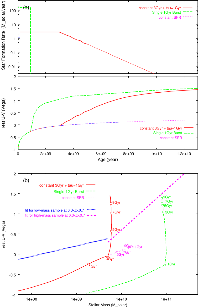
Figure 31: (a): Top: star formation rate vs age for the models with various star formation history. Constant 3Gyr SFR $+\tau=$1Gyr model with 5$\times 10^{9}$M_⊙ at 3Gyr old (solid), single 1Gyr burst with 10¹¹M_⊙ at 1Gyr old (dash), constant SFR with 5$\times 10^{9}$M_⊙ at 3Gyr old (short-dashed). Bottom: rest $U-V$ color vs age for the same models calculated from the GALAXEV library. (b): rest $U-V$ color vs stellar mass for the models in (a). Each line corresponds to each star formation history of (a). Each square represents age. Bold lines show the fitting result for the observed galaxies at $0.3<z<0.7$.

What kind of the galaxy evolution scenario can explain this trend ? If we consider the pure passive evolution for these galaxies, the $U-V$ color is expected to be bluer at higher redshift with nearly constant stellar mass. This seems to disagree with our result. For example, in Figure 31, we show the track of such a model in the rest $U-V$ color vs stellar mass plane, using the single 1Gyr burst model with 10¹¹M_⊙ at 1Gyr old (dashed line). As seen from the model, if observed high-mass galaxies follow passive evolution, the correlation between the $U-V$ color and the stellar mass shifts blue-ward with redshift especially at low mass side unless the degree of dust extinction is regulated with the stellar mass and the stellar age. In order to make the relation between the stellar mass and the rest $U-V$ color nearly constant over relatively long timescale, galaxies will have to increase their stellar mass as their stars become older. Furthermore, since the comoving volumes of $1.1<z<1.9$ bin and $1.9<z<2.7$ bin are more than three times larger than that of $0.7<z<1.1$ bin, the number density of galaxies with M${}_{stellar}\gtrsim 1\times 10^{10}$M_⊙ seems to decrease between $z\sim 1$ and $z\sim 3$, although small number statistics prevents the conclusive result. For relatively bright (probably massive) early-type galaxies, several previous studies also found that the number density of these galaxies seems to decrease at $z\gtrsim 1.4$ (Zepf, 1997; Franceschini et al., 1998; Barger et al., 1999; Menanteau et al., 1999; Treu & Stiavelli, 1999; Stanford et al., 2004, see also Daddi et al., 2000; McCarthy et al., 2001).
The merging without active star formation may be possible solution to increase the stellar mass of these galaxies. In this scenario, the observed relation corresponds that the stellar mass increases through mergers from $\sim 5\times 10^{9}$M_⊙ to $\sim 5\times 10^{10}$M_⊙ during the time when the $U-V$ color evolves from $\sim 0.4$ to $\sim 1.2$. For example, in Figure 31, we assume the model where the star formation rate is constant by the time the stellar mass reaches 5$\times 10^{9}$M_⊙, and then star formation rate decreases exponentially with characteristic time scale $\tau=$1Gyr (solid line). We consider the case that the period for which star formation rate is constant is 3Gyr. Star formation rate is adjusted such that the stellar mass becomes 5$\times 10^{9}$M_⊙ at 3Gyr old, (Figure 31(a)). In the model, after 3Gyr old, the star formation rate decreases and the stellar mass does not grow. Comparing this (no merger) model with the observed correlation between the rest $U-V$ and stellar mass, we found that in order to form the observed correlation, galaxies have to increase their stellar mass after star formation activities decrease at the rate of 2–3 times per about 2Gyr through the processes such as mergers for the assumed star formation history.

5 Summary

Using the HST WFPC2/NICMOS archival data and very deep Subaru/CISCO $K^{\prime}$-band image of the Hubble Deep Field North, we estimated the stellar mass, the rest $U-V$ color, the morphology at rest-frame optical band of $K^{\prime}$-selected galaxies, and investigated the distribution of the rest $U-V$ and morphology as a function of stellar mass back to $z\sim 3$. Following results were obtained.

• In the rest $U-V$ color vs stellar mass diagram, galaxies can be divided into two populations at M${}_{stellar}\sim 5\times 10^{9}$M_⊙. Galaxies with M${}_{stellar}\lesssim 5\times 10^{9}$M_⊙ have relatively blue rest $U-V$ color and their color does not correlate strongly with stellar mass, while at M${}_{stellar}\gtrsim 5\times 10^{9}$M_⊙, there is the trend that galaxies with higher stellar mass have redder $U-V$ color. This feature seems to hold back to $z\sim 2$.

• We could not find the significant evolution of the characteristic stellar mass at which the change of the mass dependence of the rest $U-V$ color occurs, at $0.3\lesssim z\lesssim 2$.

• The $U-V$ color of the low-mass sample become bluer gradually with redshift, from $U-V\sim 0.2$ at $z\sim 0.5$, to $U-V\sim-0.2$ at $z\sim 2$. Such a color evolution is roughly consistent with that expected from the constant SFR model with a formation redshift of $z_{f}\sim 3.5$.

• On the other hand, the strong correlation between the rest $U-V$ color and the stellar mass seen in the high-mass sample does not show significant evolution at $0.3\lesssim z\lesssim 2$, although the number density of high-mass galaxies may decrease at $z\gtrsim 1$.

• At $z\lesssim 1$, disk galaxies dominate the low-mass population, while the fraction of early-type morphology is larger in the high-mass population. Although the fraction of irregular galaxies increases, the same trend as $z\lesssim 1$ is seen at $z\gtrsim 1$.

• At $z>2$, although we can only sample the galaxies with M${}_{stellar}\gtrsim 1\times 10^{9}$M_⊙, it is seen that galaxies with higher stellar mass tend to have redder rest $U-V$ color over the mass range of $1\times 10^{9}$–$1\times 10^{10}$M_⊙.

Finally, these results about galaxy evolution are based on the HDF-N data, which is at most 4 arcmin². The field-to-field variance for such a small volume analysis is inferred to be relatively large. Although the $I-K$ vs $K$ color-magnitude diagram of several other fields suggests that the close connection between the star formation activities and the stellar mass found in our analysis could be applied to other general fields as mentioned in section 4.1, the investigation/confirmation by the larger-volume survey is clearly important, especially to reveal the evolution of high-mass galaxies, which are relatively rare and maybe strongly clustering.

Table 1: Slope value of the linear fit in the rest $U-V$ color vs $\log{M_{stellar}}$ plane

Redshift	M${}_{stellar}<5\times 10^{9}$M⊙	M${}_{stellar}>5\times 10^{9}$M⊙
0.3-0.7	0.260$\pm$0.096	1.002$\pm$0.269
0.7-1.1	0.152$\pm$0.095	0.801$\pm$0.196
1.1-1.9	0.049$\pm$0.119	0.980$\pm$0.279
1.9-2.7	0.450$\pm$0.546	0.425$\pm$0.437

Table 2: Offsets of the average rest $U-V$ color from the value at $0.3<z<0.7$

Redshift	M${}_{stellar}<5\times 10^{9}$M⊙	M${}_{stellar}>5\times 10^{9}$M⊙
0.7-1.1	-0.134$\pm$0.223	-0.115$\pm$0.274
1.1-1.9	-0.234$\pm$0.230	-0.224$\pm$0.362
1.9-2.7	-0.394$\pm$0.254

References

- Abraham et al. (1996) Abraham, R. G., van den Bergh, S., Glazebrook, K., Ellis, R. S., Santiago, B. X., Surma, P., & Griffiths, R. E. 1996, ApJS, 107, 1
- Barger et al. (1999) Barger, A. J., Cowie, L. L., Trentham, N., Fulton, E., Hu, E. M., Songaila, A., & Hall, D. 1999, AJ, 117, 102
- Bertin & Arnouts (1996) Bertin, E. & Arnouts, S. 1996, A&AS, 117, 393
- Bolzonella, Miralles & Pelló (2000) Bolzonella, M., Miralles, J M. & Pelló, R. 2000, A&A, 363, 476
- Brinchmann & Ellis (2000) Brinchmann, J. & Ellis, R. S. 2000, ApJ, 536, L77
- Bruzual & Charlot (2003) Bruzual, G. & Charlot, S. 2003, MNRAS, 344, 1000
- Calzetti et al. (2000) Calzetti, D., Armus, L., Bohlin, R. C., Kinney, A. L., Koornneef, J., & Storchi-Bergmann, T. 2000, ApJ, 533, 682
- Chabrier (2003) Chabrier, G. 2003, ApJ, 586, L133
- Cohen et al. (2000) Cohen, J. G., Hogg, D. W., Blandford, R., Cowie, L. L., Hu, E., Songaila, A., Shopbell, P., & Richberg, K. 2000, ApJ, 538, 29
- Cole et al. (2001) Cole, S., et al. 2001, MNRAS, 326, 255
- Cowie, Hu, & Songaila (1995) Cowie, L. L., Hu, E. M., & Songaila, A. 1995, AJ, 110, 1576
- Daddi et al. (2000) Daddi, E., Cimatti, A., Pozzetti, L., Hoekstra, H., Röttgering, H. J. A., Renzini, A., Zamorani, G., & Mannucci, F. 2000, A&A, 361, 535
- Dickinson (1998) Dickinson, M. 1998, The Hubble Deep Field, 219
- Dickinson (2000) Dickinson, M. 2000, Royal Society of London Philosophical Transactions Series A, 358, 2001
- Dickinson et al. (2000) Dickinson, M., et al. 2000, ApJ, 531, 624
- Dickinson, Papovich, Ferguson, & Budavári (2003) Dickinson, M., Papovich, C., Ferguson, H. C., & Budavári, T. 2003, ApJ, 587, 25
- Fontana et al. (2003) Fontana, A., et al. 2003, ApJ, 594, L9
- Franceschini et al. (1998) Franceschini, A., Silva, L., Fasano, G., Granato, G. L., Bressan, A., Arnouts, S., & Danese, L. 1998, ApJ, 506, 600
- Giallongo et al. (1998) Giallongo, E., D’Odorico, S., Fontana, A., Cristiani, S., Egami, E., Hu, E., & McMahon, R. G. 1998, AJ, 115, 2169
- Glazebrook et al. (1999) Glazebrook, K., Blake, C., Economou, F., Lilly, S., & Colless, M. 1999, MNRAS, 306, 843
- Hawarden et al. (2001) Hawarden, T. G., Leggett, S. K., Letawsky, M. B., Ballantyne, D. R., & Casali, M. M. 2001, MNRAS, 325, 563
- Kajisawa & Yamada (2001) Kajisawa, M. & Yamada, T. 2001, PASJ, 53, 833
- Kauffmann et al. (2003) Kauffmann, G., et al. 2003, MNRAS, 341, 54
- Lowenthal et al. (1997) Lowenthal, J. D., et al. 1997, ApJ, 481, 673
- McCarthy et al. (2001) McCarthy, P. J., et al. 2001, ApJ, 560, L131
- Menanteau et al. (1999) Menanteau, F., Ellis, R. S., Abraham, R. G., Barger, A. J., & Cowie, L. L. 1999, MNRAS, 309, 208
- Motohara et al. (2002) Motohara, K., et al. 2002, PASJ, 54, 315
- Papovich, Dickinson, & Ferguson (2001) Papovich, C., Dickinson, M., & Ferguson, H. C. 2001, ApJ, 559, 620
- Pei (1992) Pei, Y. C. 1992, ApJ, 395, 130
- Sawicki & Yee (1998) Sawicki, M. & Yee, H. K. C. 1998, AJ, 115, 1329
- Shapley et al. (2001) Shapley, A. E., Steidel, C. C., Adelberger, K. L., Dickinson, M., Giavalisco, M., & Pettini, M. 2001, ApJ, 562, 95
- Stanford et al. (2004) Stanford, S. A., Dickinson, M., Postman, M., Ferguson, H. C., Lucas, R. A., Conselice, C. J., Budavári, T., & Somerville, R. 2004, AJ, 127, 131
- Steidel et al. (1999) Steidel, C. C., Adelberger, K. L., Giavalisco, M., Dickinson, M., & Pettini, M. 1999, ApJ, 519, 1
- Treu & Stiavelli (1999) Treu, T. & Stiavelli, M. 1999, ApJ, 524, L27
- van den Bergh, Cohen, Hogg, & Blandford (2000) van den Bergh, S., Cohen, J. G., Hogg, D. W., & Blandford, R. 2000, AJ, 120, 2190
- Wirth et al. (2004) Wirth, G. D., et al. 2004, AJ, 127, 3121
- Yamada et al. (2001) Yamada, T., et al. 2001, PASJ, 53, 1119
- Zepf (1997) Zepf, S. E. 1997, Nature, 390, 377