Fourier transform method for imaging atmospheric Cherenkov telescopes

Abstract

We propose Fourier transform (hereafter FT) method for processing images of extensive air showers (EAS) detected by imaging atmospheric Cherenkov telescopes (IACT) used in the very high energy (VHE) gamma-ray astronomy. The method is based on the discrete Fourier transforms (DFT) on compact Lie groups, and the use of continuous extension of the inverse discrete transform for approximation of discrete EAS images by continuous EAS brightness distribution functions. Here we present the FT-method for SU(3) group. It allows practical realization of the DFT method for functions sampled on hexagonal symmetry grids implemented in most of the current IACT cameras. We note that the proposed FT-method can also be implemented for the rectangular grids using the DFT on $\rm SU(2)\times SU(2)$ group.

We present the results of application of the FT-method to Monte-Carlo simulated bank of TeV proton and gamma-ray EAS images for a stand-alone telescope. Comparing between the FT-method and the currently used standard method for signal enhancement, on the basis of parameter ALPHA, shows that the FT technique allows a better and systematic increase of the gamma-ray signal. The relative difference between these two methods becomes more profound especially for ‘photon poor’ images, for which the standard method deteriorates. It suggests that the EAS detection thresholds could be effectively reduced with implementation of the FT technique for IACTs. This prediction is further supported by a significant noise suppression capability of the method using simple ‘low-pass’ filters in the image frequency domain. This new approach allows very deep ‘tail’ (and ‘height’) image cuts, differentiation of images, frequency spectra, etc., which can be used for development of new effective parameters for the EAS image processing.

1 Introduction

Since last 15 years, starting from the first confident detection of the Crab Nebula  [1], the IACTs have proved powerful detectors of very high energy (VHE, conventionally $E\geq 100\,\rm GeV$) gamma-rays sources. Due to IACTs, and in particular, stereoscopic IACT systems (see  [2]), VHE gamma-ray astronomy is now an established and rapidly growing observational astronomy, with proven experimental methodology and with already significant number of detected sources of various types (see  [3] for the comprehensive recent review). As well known, the power of IACTs is based on the realization of the idea  [4] that extensive air showers (EAS) induced by cosmic rays (CRs) and gamma-rays can be effectively discriminated from each other exploiting the intrinsic differences between their Cherenkov light images detected by the multichannel optical photoreceivers (cameras) of the telescopes.

The standard method (hereafter, S-method) for such image discrimination involves various ”shape” and ”orientation” parameters proposed first by Hillas  [5], which are based on the first and second-order moments of the EAS image $\{G_{J}\}$. Recall that the EAS image is a set of numbers $G_{J}$ of photoelectrons registered by the $J$-th photomultiplier tubes (PMTs) of the IACT camera. The integer index $J=1,2,...,K$ corresponds to the discrete 2-dimensional spatial (angular) coordinates of the PMTs, $J=(j,m)$. In order to improve the performance of the ‘standard parameterization’, different image preprocessing techniques have been suggested (e.g.  [6, 7, 8]). Note that all of these image filtering methods are based on the image processing directly in the coordinate (i.e. image) space.

Meanwhile, one of the known powerful methods used for signal processing generally is the method of discrete Fourier transform (DFT; see e.g.  [9, 10]). In this method the discrete image is transformed into wave number (or frequency, for transformation of the time argument) space, in which different ‘filters’ can be applied. Then the filtered image is recovered by the inverse transform. Yet, this approach has not been implemented for the EAS images detected by IACTs. Perhaps, it could be partly explained by the hexagonal/triangular symmetry of the PMT grids implemented in most of the current IACTs, whereas the known methods of DFT are developed for images defined on grids of rectangular symmetry.

Here we propose a method which allows DFT of 2-dimensional images sampled on hexagonal grids. This technique represents a particular case of implementation of a general method for Fourier analysis of multidimensional discrete functions which uses the so called orbit functions of compact Lie groups as the transform basis  [11, 12, 13]. To distinguish it from standard DFT, we abbreviate the DFT on Lie groups as DGT, standing for discrete group transform. Images defined on grids with hexagonal symmetry belong to the case of Fourier transform on the group SU(3), whose root lattice displays that symmetry. In Section 2 we show that the method is rather simple and can be used in practice even without any specific knowledge of the Lie group theory.

Note that the case of DGT on the group SU(2), which has been considered in detail in  [14], is reduced to a specific type of DFT known earlier as discrete cosine transform (DCT, see  [15]). The 2-dimensional version of DCT is notorious as the basis for the high-performance image compression standard JEPG. It corresponds to DGT on the Lie group SU(2)$\times$SU(2), and allows processing of images sampled on the ordinary rectangular grids. Thus, although in this paper we describe the Fourier transform method (hereafter, FT-method) for the IACTs with hexagonal symmetry of the PMT grids used in most of current IACTs  [16, 17, 18, 19], the FT-method is equally applicable for IACTs with the grids of rectangular symmetry (e.g.  [20]).

Our previous study of DGTs has shown that these transforms are distinguished by some valuable properties. In particular, the inverse DGTs can be treated as continuous Fourier polynomials, or continuous extensions (CE) of the discrete transform which interpolate well the discrete image at any point between the grid. Unlike continuous extensions of the standard DFT, but very similar to the canonical continuous Fourier transform polynomials, the CEDGTs are converging functions. Furthermore, the known properties of localization and differentiability of the continuous Fourier transform series hold for CEDGT polynomials as well (see  [14]).

After describing in Section 2 the basic mathematical technique of the Fourier transform on the Lie group SU(3) and demonstrating the ability of CEDGT to approximate the original analytic functions, in Section 3 we apply this technique for interpolation of Monte-Carlo (M-C) simulated images of gamma-ray and proton induced EAS. The goal of this paper is first of all to present the Fourier transform method itself and to discuss some of the related new possibilities for the IACT image processing, rather than achieving the best result for the contemporary stereoscopic IACT arrays. Therefore here we use EAS images simulated for a stand-alone IACT with parameters for both the camera and the collector corresponding to those of the HEGRA telescopes (see  [22]). It assumes a hexagonal 271-PMT camera with angular size of PMTs $h=0.25^{\circ}$, and the telescope collector area $\simeq 8.5\,\rm m^{2}$. These relatively modest parameters result in comparatively coarse (‘poor’) images. For such images the performance of the proposed FT-method, which consists in Fourier transformation and then interpolation of discrete images by CEDGT, is significantly better than the performance of the S-method.

In Section 4 we discuss some possibilities for image processing in the frequency domain that can be opened with the use of the FT-method. These possibilities include ‘denoising’ of the image by cutting off the highest frequency harmonics before the use of CEDGT. This is a very simple low-pass filtering procedure which, nevertheless, appears rather effective for practical purposes. We will also demonstrate here, although only qualitatively rather than quantitatively (which would require a separate detailed study) that the proposed “functional” approach contains a significant potential for reducing the effective energy threshold of the IACTs.

Throughout this paper the comparing with the S-method is done only on the basis of parameter ALPHA which has proved to be a very efficient single parameter used in the ‘standard parameterization’. In order to keep this comparison straightforward, in this paper we refrain from introducing new parameters for image discrimination, which in principle would be possible having a continuous function instead of a discrete image.

2 Fourier transforms on SU(3)

2.1 SU(3) Fourier transform on a grid

In general terms, the concept ‘Fourier transform on a grid’ means that a discrete function $\{G_{k}\mid k=0,1,...,K\}$ defined on the vector points $\{{\bf r}_{k}\mid k=0,1,...,K\}$ of a grid in $\mathbb{R}^{2}$ (or generally in any $n$-dimensional real space $\mathbb{R}^{n}$), can be represented as a linear combination of wave functions $e^{i({\bf k}_{i}\cdot{\bf r})}$ sampled on the same grid. The set of wave numbers (or ‘frequencies’ in case of time variable) involved is finite, i.e. $\{{\bf k}_{i}\mid i=0,1,...K^{\prime}\}$, where $K^{\prime}$ is not necessarily equal to $K$. It is important, however, that the action of the transform operator $\hat{T}$ would produce an unambiguous ‘image’ of $\{G_{k}\}$ in the wave vector space, $\hat{T}\,:\,\{G_{k}\}\rightarrow\{A_{j}\mid j=0,1,...,K_{1}\}$ where $K_{1}=K$. Since the transform operator is linear, the numbers of independent elements in the original and transformed images should be equal.

The method of DFT on compact Lie groups, or the DGT, is based on two principal ingredients suggested in  [11, 12] which allow practical computation of Fourier transforms on Lie groups. These are the discretization of the space of variables in accordance with the elements of finite order (EFO) of the group, and the use of orbit functions of the group as the transform basis. The basic property that makes the method work, is the orthogonality of the orbit functions on the sets of EFOs (see  [11, 12, 13] for details). The EFOs of adjoint orders dividing an integer $N$ make a discrete grid of a definite symmetry (depending on the group) in the so called fundamental region of the group.

Without going into specific mathematical details, which are being presented elsewhere, but in order to show the connection between the transform basis and the Lie groups, we remind that the group SU(3) can be faithfully represented as the group of all unitary matrices of size $3\times 3$. Any unitary matrix can be diagonalized by a unitary transformation. Therefore every element of SU(3) is conjugate to at least one diagonal element $\Theta$ in this 3-dimensional matrix representation. The set of all such diagonal matrices forms the maximal torus T of the group:

$${\sf T}=\left\{\Theta(x,y,z)=\left(\begin{array}[]{ccc}e^{2\pi ix}&0&0\\ 0&e^{2\pi iy}&0\\ 0&0&e^{2\pi iz}\end{array}\right)\;\mid\;x+y+z=0\right\}\;.$$ (1)

The condition $x+y+z=0$ describes a plane on which the unitary condition $\det{\Theta}=1$ for the matrices is satisfied. Every element of the group can be thus represented by a 2-dimensional vector point on this plane. In particular, the simple roots of SU(3), given by vectors $\alpha_{1}=(1,-1,0)$ and $\alpha_{2}=(0,1,-1)$, correspond to the 2-dimensional vectors with lengths equal to $\sqrt{2}$ at an angle $120^{\circ}$ to each other. In that plane, the maximal torus T of the group corresponds to the hexagonal region shown in Fig. 1a.

Two elements in T are conjugate, if and only if they differ by permutation of their diagonal entries. The conjugacy classes in SU(3) are in 1-1 correspondence with the points in the fundamental domain F of the group. In Fig. 1 it corresponds to the triangular segment enclosed between vectors $\omega_{1}$ and $\omega_{2}$ representing the fundamental weights of SU(3). These vectors are expressed through $\alpha_{1}$ and $\alpha_{2}$ as $\omega_{1}=(2\alpha_{1}+\alpha_{2})/3$ and $\omega_{2}=(\alpha_{1}+2\alpha_{2})/3$. The weights $\omega_{1}$ and $\omega_{2}$ are orthogonal to $\alpha_{2}$ and $\alpha_{1}$, respectively, with the scalar product $(\omega_{i}\,,\alpha_{j})=\delta_{i,j}$, where $\delta_{ij}$ is the Kroneker symbol.

Any vector $\lambda$ in the plane can be expressed through fundamental weights as $\lambda=a\omega_{1}+b\omega_{2}$. Action of the Weyl group $W$ on $\lambda$, which in case of SU(3) group is reduced to reflections of $\lambda$ in the lines of vectors $\omega_{1}$ and $\omega_{2}$, produces a finite set $\{W(\lambda)\}$ of vectors equidistant from the origin. This set represents the Weyl group orbit of $\lambda$ containing the following 6 elements $\mu$:

$$W(\lambda) = \{a\omega_{1}+b\omega_{2}\>,\>b\omega_{1}-(a+b)\omega_{2}\>,\>-(a+b)\omega_{1}+a\omega_{2}\>,$$ (2)

$$\;\>-a\omega_{1}+(a+b)\omega_{2}\>,\>(a+b)\omega_{1}-b\omega_{2}\>,\>-b\omega_{1}-a\omega_{2}\,\}$$

In particular cases, when either $a=0$ or $b=0$, the number of different elements in Eq.(2) is reduced from 6 to 3 (see Fig. 1a), and it is only 1 if $a=b=0$. Note that the action of the Weyl group expands the fundamental region F onto the maximal torus T.

An orbit function $\Psi_{(\lambda)}\equiv\Psi_{a,b}$ at the vector point $r$ (hereafter we use this simple notation instead of r) is defined  [11, 12] as a finite sum of exponential functions on the Weyl group orbit of the element $\lambda$:

$$\Psi_{a,b}(r)=\sum_{\mu\in W(\lambda)}e^{2\pi i(\mu,r)},$$ (3)

where $(\mu,r)$ is the scalar product of 2 vectors. Here we will be interested in orbit functions corresponding to integer indices $a$ and $b$.

An EFO is an element $X$ of the group, such that $X^{N}$ is the unit element $E$ for some natural number N. In the $\omega$-basis representation $X=a_{1}\omega_{1}+b_{1}\omega_{2}$ this condition is satisfied if (and only if) $a_{1}$ and $b_{1}$ are rational numbers. The sets of all EFOs of adjoint order dividing $N$ are represented by vector points $X\rightarrow{r}_{k,m}$ with $a_{1}=k/N$ and $b_{1}=m/N$ that satisfy the conditions $0\leq k,m,k+m\leq N$. These make sets $\{r_{km}\}\equiv{\sf F}_{N}\subset{\sf F}$ in the form of equilateral triangular grids, as shown in Fig. 1b for $N=12$.

The key property for the method of DFT on compact semisimple Lie groups is the discrete orthogonality of orbit functions with different $\lambda$ on the sets ${\sf F}_{N}$ of EFOs of adjoint order $N$  [11, 12]. In case of SU(3) group this property corresponds to the equation

$$\sum_{r_{km}\in{\sf F}_{N}}P_{km}\Psi_{j,n}(r_{km})\overline{\Psi_{i,p}}(r_{km})=\delta_{i,j}\delta_{p,n}\,D_{N}(j,n)$$ (4)

where

$$P_{km}=\frac{6}{(1+\delta_{k+m,0})(1+\delta_{k,0}+\delta_{m,0})}\;,$$ (5)

is a multiplicity factor, and the Kroneker symbols are treated modulo N, i.e. $\delta_{i,j}=1$ if $i=j$ mod($N$), e.g. $\delta_{N,0}=1$. The normalization factor in Eq.(4) is

$$D_{N}(j,n)=\frac{108N^{2}}{P_{jn}}\;,$$ (6)

Important statements for the method of DFT on Lie groups  [11, 12] are the following two:
(a) for any given $N$ the set of orbit functions $\Psi_{j,n}$ with indices $0\leq j,n,j+n\leq N$ makes a full set of functions orthogonal to each other on the equilateral triangular grid $\{r_{km}\mid 0\leq k,m,k+m\leq N\}$ in the form of Eq.(4);
(b) this set provides a basis for DGT on SU(3) orbit functions with the smallest possible wave numbers $(j,n)$.

A DGT of a given discrete function $\{G_{km}\equiv G(r_{km})\}$ produced by sampling of a continuous (analog) function $G(r)$ at the grid points $\{r_{km}\}$ corresponds to solution of the set of equations

$$G_{km}=\sum_{j,n\geq 0}^{j+n\leq N}A_{jn}\Psi_{jn}(r_{km})\;\;{\rm for}\;\;0\leq k,m,k+m\leq N\,.$$ (7)

Multiplying Eq.(7) by $P_{km}\overline{\Psi_{ps}}(r_{km})$, then summing up over $\{k,m\}$, and using Eq.(4), the transform values $\{A_{jn}\}$ are readily found:

$$A_{jn}=\frac{1}{D_{N}(j,n)}\sum_{k,m\geq 0}^{k+m\leq N}P_{km}G_{km}\overline{\Psi_{jn}}(r_{km}).$$ (8)

2.2 Continuous extension of DGT

The set $\{A_{km}\,\mid\,0\leq k,m,k+m\leq N\}$ is an exact Fourier transform of $\{G_{km}\}$, as far as the knowledge of $\{A_{km}\}$ allows unambiguous reconstruction of $\{G_{km}\}$ at the points $\{r_{km}\}$ of the given grid using the inverse DGT, i.e. Eq.(7).

The inverse DGT can be extended into a continuous function in the form of Fourier polynomial (i.e. a series of cosine and sine functions) as suggested in  [14]. It is done simply by replacing the discrete spatial argument $r_{km}$ of the orbit functions $\Psi_{jn}(r_{km})$ in the inverse DGT series, Eq.(7), by the continuous argument $r$. The resulting function

$$F_{N}(r)=\sum_{j,n\geq 0}^{j+n\leq N}A_{jn}\Psi_{jn}(r)$$ (9)

is called continuous extension of DGT, or CEDGT. Note that in case of real functions, $F_{N}(r)$ is reduced to $\sum_{\{j,n\}}[\,{\rm Re}A_{jn}\,{\rm Re}\Psi_{jn}(r)-{\rm Im}A_{jn}\,{\rm Im}\Psi_{jn}(r)\,]$.

The function $F_{N}(r)$ coincides, obviously, with $\{G_{km}\}\equiv G(r_{km})$ at the grid points. However, the most valuable property of $F_{N}(r)$ is in the quality of its interpolation of the values $G_{km}$ between the grid points. The approximation to the original $G(r)$ that it provides is such that even the first and (under certain conditions) also the second derivatives of $F_{N}(r)$ are meaningful functions, converging to the respective derivatives of $G(r)$. The CEDGT also satisfies the property of locality of the transform. These are similar to the properties of canonical continuous Fourier transforms. Note that these properties do not hold, however, for the continuous extension of the traditional version of DFT (i.e. which is often used in case of rectangular grids). Even the straightforward continuous extension of the ordinary DFT is a meaningless (profoundly oscillating) function (see  [14] for details).

For convenience here we write the explicit expressions for the SU(3) orbit function $\Psi_{a,b}(r)$. In Cartessian coordinates with the $y$-axis bisecting the equilateral triangle (i.e. the fundamental region), with the sides of length 1, as in Fig. 1b, the real and imaginary parts of the orbit functions are reduced to the following:

$${\rm Re}\,\Psi_{a,b}(x,y) = \;\;2\,\cos\left(2\pi y\frac{a+b}{\sqrt{3}}\right)\cos\left(2\pi x\frac{a-b}{3}\right)$$

$$+\>2\,\cos\left(2\pi y\frac{a}{\sqrt{3}}\right)\cos\left(2\pi x\frac{2b+a}{3}\right)$$

$$+\>2\,\cos\left(2\pi y\frac{b}{\sqrt{3}}\right)\cos\left(2\pi x\frac{2a+b}{3}\right)\;,$$

$${\rm Im}\,\Psi_{a,b}(x,y) = \;\;2\,\cos\left(2\pi y\frac{a+b}{\sqrt{3}}\right)\sin\left(2\pi x\frac{a-b}{3}\right)$$

$$+\>2\,\cos\left(2\pi y\frac{a}{\sqrt{3}}\right)\sin\left(2\pi x\frac{2b+a}{3}\right)$$

$$-\>2\,\cos\left(2\pi y\frac{b}{\sqrt{3}}\right)\sin\left(2\pi x\frac{2a+b}{3}\right)\;.$$

In this system of coordinates, the property of complex conjugation of orbit functions $\Psi_{a,b}=\overline{\Psi_{b,a}}$ results in useful symmetry properties of the real and imaginary parts with respect to variables $x$ and $y$. Also, if $a=b$, then ${\rm Im}\,\Psi_{a,a}(x,y)=0$. Note that in case of integer $a$ and $b$ the harmonic order of these polynomials is not always integer.

2.3 Examples of CEDGT for analytic functions sampled on grids

The interpolation power of continuous extensions of DGTs is demonstrated in Fig. 2. For an example, here we interpolate a function sampled on a rectangular grid. The appropriate Lie group for this symmetry is SU(2)$\times$SU(2). The DGT in this case happens to result in 2-dimensional case of a transform known as DCT (discrete cosine transform). The orbit functions of the SU(2) group, for a one-dimensional function, are composed only of 2 exponents, $\Psi_{\lambda}(\theta)=e^{i2\pi\,\lambda\theta}+e^{-i2\pi\,\lambda\theta}=2\cos(2\pi\lambda\theta)$ with $\theta\in[0,1/2]$  [14]. The basis for the two-dimensional DCT simply is a product of 2 cosine functions in 2 orthogonal directions in the plane.

The discrete image shown in Fig. 2a is produced from sampling of the original analytic function $G(r)$ composed of a sum of two 2-dimensional Gaussian distributions with large axes inclined at an angle 25^∘ to each other. The characteristic widths of both are chosen to be smaller than the distance between the grid points, and correspond to dispersions $\sigma_{\perp}=2/3N$. This grid is rather sparse for the image, which is apparent on Fig. 2a. The result of application of CEDGT is demonstrated in Fig. 2b (panel on the right). The original function is recovered almost exactly, clearly separating the 2 ellipsoids and recovering their orientations. The only noticeable difference between CEDGT function $F_{N}(r)$ and the original $G(r)$ is reduced to some low-amplitude wiggles. In Fig. 2b these wiggles result in the appearance of the dashed contour line corresponding to the level of $-0.1\%$ of the maximum intensity in the image.

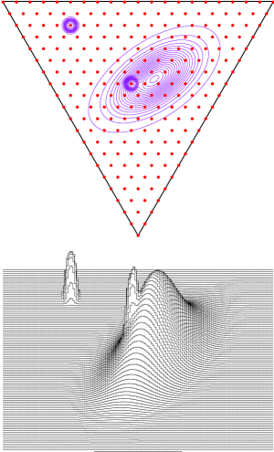
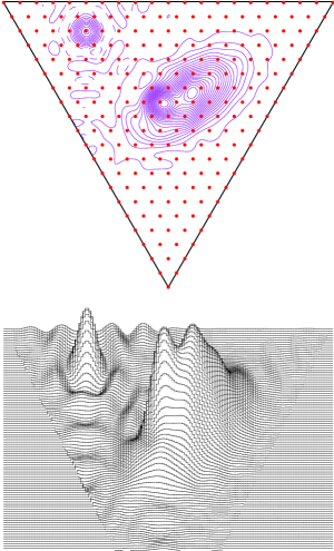
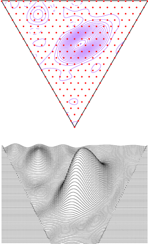
Figure 4: a (2 panels on the left):  The contour plot (upper panel) and the 3-dimensional view of an analog image composed of 2-dimensional continuous Gaussian ellipsoid, onto which 2 narrow spikes which produce 2 ‘hot pixels’ (after sampling of the analog signal on the grid) are superimposed. The heights of the spikes are equal to half of the height of the ellipsoid;  b  (2 panels in the middle):  A direct (i.e. without filtering) CEDGT interpolation of the discrete image produced by sampling of the analog image on the grid with $N=20$;  c (2 panels on the right):  CEDGT view of the image after application of the filter with $C_{f}=0.5$ (see text).

It should be noted that a straightforward interpolation of discrete images by CEDGT can be useful in case of low level of noise in the signal, but it may be less effective if the level of noise is high. This is because the CEDGT ‘zooming’ of an image containing random noise makes the latter more apparent at small spatial scales. In this regard, an important property is that the Fourier transform of an additive random (‘white’) noise also is a random noise, whereas the DGT representation $\{A_{jn}\}$ of any meaningful image is concentrated in the domain of long frequency harmonics (e.g. see  [15]). That is, the coefficients $\mid A_{jn}\}\mid$ have a general tendency to decrease with the increase of $j$ and $n$. Therefore the noise typically becomes relatively stronger, and even may completely dominate the signal at high frequencies, as demonstrated in Fig. 3. The big dots here correspond to the mean absolute values $\mid A_{km}\mid$ of the transform coefficients of different harmonic orders $K=k+m\leq N$ for an image presented in Fig. 4a. The stars show the mean values of the DGT coefficients of the noise (contributed by 2 ’hot pixels’ described below in Fig. 4) in this image alone. It is obvious that at high frequencies $K\geq N/2$ the the DGT image is totally dominated by this noise.

This property can be exploited for organizing a very simple, but also very effective, low-pass filter. Namely, we can cut off in the frequency domain all modes $A_{km}$ of harmonic orders exceeding some large $N_{cut}$, i.e. putting $A_{km}\rightarrow 0$ for indices $N_{cut}<K=(k+m)\leq N$. Then we can use the truncated CEDGT series that contains only the modes $K\leq N_{cut}$ to approximate the image. This filter can be described by a parameter $C_{f}=1-N_{cut}/N$ such that $C_{f}=0$ corresponds to ”no filtering”.

The result of application of such low-pass filter is shown in Fig. 4. The original image in Fig. 4a corresponds to continuous function in the form of 2-dimensional Gaussian distribution with effective width $\sigma_{\perp}=1/N=0.05$ and length $\sigma_{\parallel}=2\sigma_{\perp}$. Onto it 2 isolated ‘hot pixels’, with heights of each equal to the half of the maximum of the main image, are superimposed. One of the ’hot pixels’ is chosen far from the main structure, but the second one falls within the image close to its maximum. This results in the total signal in that pixel exceeding the maximum value of the main function.

Fig. 4b (panels in the middle) demonstrates the result of straightforward extension of the discrete image using CEDGT without filtering. Note that the amplitude of oscillations of the hexagonal Fourier waves in the near vicinity of the isolated ‘hot pixel’ may reach up to $\simeq 15$-$20\,\%$ of the ‘hot pixel’ value. The distance between the contour lines corresponds to $5\,\%$ of the maximum of the ellipsoid, and dashed contours correspond to the negative values of the CEDGT image. Note that the amplitude of the oscillations rapidly declines with distance from the ‘hot pixel’ because of the localization property of the CEDGT  [14].

In Fig. 4c we show the result of application of the low-pass filter with the filtering parameter $C_{f}=0.5$. The main signal practically does not change. This is because for the original images with effective widths $\sigma_{\perp}\geq 1/N$, the Fourier transformed ‘image’ $\{A_{km}\}$ is concentrated mostly in the domain of low wave numbers $(k+m)\leq N/2$, as shown in Fig. 3. Note that even for more narrow images, with widths about only one half of the size of pixels in the grid, $\sigma_{\perp}\simeq 1/2N$, the amplitude of the image after filtering with $C_{f}=0.5$ drops only by $\sim 25$-$30\,\%$, but the orientation of the original images is recovered quite well. Meanwhile, both ”noisy pixels” have almost disappeared from the filtered image in the Figure 4c. The signal in the isolated pixel has dropped by a factor $\sim 4$. Even more important is that the intensity in the ‘hot pixel’ inside the main body of the image has practically recovered the expected value of the signal. The difference between the contours in Figures 4a and 4c is mostly at contour levels corresponding to low intensities. This difference can be completely eliminated by modest ‘tail’ cuts, which is the standard image pre-processing procedure discarding the pixels with signals below some level, or perhaps even more effectively, by the ‘height’ cuts as we explain below in Section 3.

3 Performance of the FT method

To compare relative performances of the FT- and S- methods, Monte-Carlo data bank for proton and gamma-ray primaries has been simulated using Hillas’ MOCCA code  [23] complemented with the full ray-tracing of the incident Cherenkov photons  [24]. The IACT parameters, such as photocollector radius/size, altitude, etc., have been assumed corresponding to the telescopes of the HEGRA system located at $2200$ m above sea level (see  [22]). In particular, the images are formed in the plane of photoreceiver consisting of 271 PMTs (or pixels), with the angular size $h=0.25^{\circ}$ arranged in the hexagonal grid. This grid is relatively coarse compared to the cameras of the contemporary IACT projects, and also the number of PMTs is relatively modest. Both these factors do help, however, to compare and reveal more easily the differences between the FT- and S- methods.

For both proton and gamma-ray events, the showers have been generated with energies starting from $0.3\rm TeV$, which is significantly lower than the detection threshold of IACTs with the given parameters. The simulations were performed for a telescope pointed to the zenith. The gamma-ray EAS with power-law index of the primary photon spectrum $-2.6$ are generated in the vertical direction, i.e. parallel to the telescope optical axis. For the CR protons, an isotropic distribution within a vertical cone with the opening (half-) angle $\leq 2.7^{\circ}$, and with the spectral index $-2.67$ has been used. The trigger condition for EAS detection was chosen as ‘2nn/217 $\geq 10\,pe$’, i.e. $\geq 10$ photoelectrons in any 2 near neighbors from 217 inner PMTs. This excludes the PMTs of the last (hexagonal) ring from the trigger. In our data bank the number of proton EAS passing the trigger is $N_{p,tot}=2354$, and $N_{\gamma,tot}=4229$ for gamma-ray events.

3.1 CEDGT representation of the EAS images

In order to apply the DGT, we have to embed the hexagonal grid of the camera into the equilateral triangular grid, i.e. into the fundamental domain of SU(3), as it is shown in Fig. 5. The camera with 271 pixels contains $M=9$ ‘hexagonal rings’ of PMTs around the central PMT. We formally add one more ring assuming $S_{km}=0$ for the numbers of photoelectrons there. It gives some additional space for processing images that may contain non-zero numbers of photoelectrons in the 9-th ring of the camera. All this results in a grid ${\sf F}_{N}$ having $N=30$ equal intervals, and $N+1=31$ grid points, along the 2 principal non-orthogonal axes $\omega_{1}$ and $\omega_{2}$ of the triangle.

Our next step is to reconstruct the values $G_{km}$ for the photoelectron distribution (the Cherenkov light brightness) function $G(r)$ at the grid points $r_{km}$. This is a useful pre-processing procedure, as far as the numbers $S_{km}$ in the detected image represent the values of photoelectrons integrated over the surface of each individual PMT. Therefore $S_{km}$ represents only the mean of the continuous distribution function over the PMT, and only in the 0-th order approximation it represents the real brightness distribution $G(r_{km})\equiv G_{km}\simeq S_{km}/s_{\rm pix}$ in the centres of PMTs. Here $s_{\rm pix}$ is the PMT surface in square angular units, which can be chosen as a normalization factor, i.e. $s_{\rm pix}=1$.

The values $G_{km}$ are better recovered if we assume that $G(r)$ is a continuous function that can be approximated within each PMT by 2-dimensional Taylor series around its centre $r_{km}$. Integrating over the hexagonal surface of the PMT, we arrive at an expression that connects the set $\{G_{km}\}$ with $\{S_{km}\}$ through the second-order derivatives of $G(r)$ at the grid point $r_{km}$:

$$G_{km}\approx\frac{S_{km}}{s_{\rm pix}}-\frac{5h^{2}}{54}\,[G^{\prime\prime}_{x}(r_{km})+G^{\prime\prime}_{x+60}(r_{km})+G^{\prime\prime}_{x-60}(r_{km})]\;.$$ (12)

Here $G^{\prime\prime}_{x}$, $G^{\prime\prime}_{x+60}(r_{km})$ and $G^{\prime\prime}_{x-60}(r_{km})$ are the second derivatives of $G(r)$ along the $x$-axis and along the directions of fundamental weights $\omega_{1}$ and $\omega_{2}$ of the equilateral triangular grid, respectively, i.e. at the angles $\pm 60^{\circ}$ relative to the $x$-axis (see Fig. 1b). This equation allows fast iterations, approximating initially the derivatives of the grid functions in the standard difference scheme approach as $f^{\prime\prime}(r_{0})=[f(r_{0}+h)+f(r_{0}-h)-2f(r_{0})]/h^{2}$. Here the notations $+h$ and $-h$ indicate the positive and negative shifts, respectively, in the given direction along the grid from the grid point $r_{0}$. For the subsequent iterations the derivatives are calculated using directly the CEDGT function. This approach provides a good agreement between the integrals of the brightness distribution function and the total numbers $\{S_{km}\}$ in the PMTs already after the second iteration. The agreement better than $\leq 1\,\%$ for most pixels, except for some (but not all) of those with very low numbers $S_{km}$. The total number of photoelectrons in the image is preserved within $\leq 1$-2 % accuracy.

In Fig. 5 we show the images of a $E=1\,\rm TeV$ gamma-ray EAS incident at a distance 130m from the telescope. Fig.5a (panel on the left) shows the raw image detected by the camera, and Fig.5b (panel in the middle) shows the continuous distribution function provided by CEDGT. Note that the lowest contour shown corresponds to the level of 3% from the maximum value of the image. It demonstrates that the ripples of the Fourier waves are very significantly eliminated already at this very low cutoff level. In Figure 5c the image is reconstructed after application of the low-pass filter with parameter $C_{f}=0.35$. The image here is unified into an essentially single-core pattern, as expected for the gamma-ray events. The contour levels in Figure 5c are at the same absolute values as in Figure 5b. Comparing with the contours in Figure 5b shows a drop in the amplitude of the maximum by $\sim 40\%$. This is because in this particular image the signal in one of the pixels was much higher than in all of its nearest neighbors. The filter accepts that as a (statistical) fluctuation and smooths it out. The total number of photoelectrons in this image makes in fact $\simeq 85\%$ of the original $S_{tot}$.

Figure 6 shows the results of application of the same filter with $C_{f}=0.35$ to the image of a proton EAS with energy $E=2\,\rm TeV$ falling at a distance $100\,m$ from the telescope. The maximum of the filtered distribution in Figure 6c is about $85\,\%$ of the unfiltered CEDGT image, and the total number of photoelectrons found after integration of the filtered image is about $90\%$ of the original $S_{tot}$. This implies that the effective width of the filtered image becomes somewhat larger than of the original. The most important feature is, however, that unlike the gamma-ray image, the proton image shows the main EAS core but it is still far from unification into a single-core pattern. Two distinct ‘islands’, presumably connected with the EAS pions, are still apparent.

3.2 Application to ‘pure’ EAS images

The efficiency of the FT-method for signal enhancement is compared with the S-method using the orientation parameter ALPHA. This parameter is chosen since it is known as one of the most effective parameters (along with AZWIDTH) currently used for the IACT image processing in the standard parameterization scheme. It is also known that ALPHA corresponds to the deflection angle of the image major axes from the direction to the central pixel of the camera viewed from the image centre of mass (i.e. from the presumed source direction, see e.g.  [21]). The signal enhancements provided by FT- and S- methods at different levels of tail-cuts $c$ and ALPHA-’cuts’ (i.e. chosing ALPHA$\leq\alpha$), are compared in terms of Q-factors, $Q\equiv Q(c,\alpha)=\eta_{\gamma}/\sqrt{\eta_{p}}$. Here

$$\eta_{\gamma}\equiv\eta_{\gamma}(c,\alpha) = \frac{N_{\gamma}(c,\alpha)}{N_{\gamma,tot}}\;,$$ (13)

$$\eta_{p}\equiv\eta_{p}(c,\alpha) = \frac{N_{p}(c,\alpha)}{N_{p,tot}}\;$$

are the fractions of gamma-ray and proton EAS, respectively, which remain in the pool after corresponding parameter cuts $c$ and $\alpha$. The maximum values $Q_{\rm max}$ are calculated by applying first a fixed tail-cut, and then varying parameter $\alpha$. Note that we consider only $Q$-factors which preserve at least $50\%$ of the initial gamma-ray events $N_{\gamma,tot}$, i.e. $\eta_{\gamma}\geq 0.5$.

To calculate the FT-image, we first reconstruct the values $\{G_{p}\}$, using Eq.(12), for the continuous distribution function of photoelectrons in the centres of PMTs that would correspond to the total numbers of photoelectrons $\{S_{p}\}$ in the image. Here the subscript $p=1,2,...P$ stands for the grid coordinates $(i,j)$ of each of $P$ pixels involved in the image. The Fourier transform coefficients $A_{i,j}$ are calculated, and the coefficients which do not pass the given filter $C_{f}$ are discarded from the CEDGT series of Eq.(9). Using this truncated CEDGT function, the values of the brightness distribution $\{G_{k}\mid k=1,2,...,K\}$ with $K\gg P$ can be calculated for a new grid with any higher density of points. For our calculations we divide each of the 6 equilateral triangles of the hexagon (the PMT surface) into 4 equal sub-triangles, and calculate the values $G_{k}$ in the centers of each of these sub-triangles. Thus, the density of points in the new image is increased by a factor 24. This also leads to an increase of the total number of points in the image approximately (because of some zeros) by the same factor, i.e. $K\simeq 24\,P$. After that a ”tail cut” (or ”height cut”, see Section 3.3) procedure is applied, i.e. $G_{k}\rightarrow 0$ if $G_{k}<g_{cut}$

Note that here we implement a slightly modified than the currently used tail cut procedure. Namely, the tail cut level $g_{cut}$ is not fixed to some value that is the same for all images, as in the standard procedure. Instead, for each image we use the ”percentage cut”, where the cut level $g_{cut}=c\times G_{max}$ is defined as a fraction $0\leq c<1$ from the image maximum $G_{max}$ to cut, but where this fraction is now fixed. This procedure takes better into account that the amplitude of possible wiggles in the CEDGT function would linearly increase with $G_{max}$. In order to make comparing with the S-method more unambiguous, we also use the same ”percentage cut” approach for the S-method. We have checked that the maximal Q-factors reached in the S-method in case of both of these tail-cut schemes are practically the same. Note also that in order to reduce the impact of statistical fluctuations due to limited numbers of events in the $(c_{i},c_{i}+\Delta c;\,\alpha_{j},\alpha_{j}+\Delta\alpha)$-bins, we first apply a standard technique of averaging of the numbers of events in the bins in the $(c,\alpha)$ plane over $(3\times 3)$ square window of bins centered at the given $(i,j)$-bin. Only then the Q-factors are calculated. This procedure makes all the results more systematic, and therefore more conclusive.

In Figure 7a we present the results of application of the FT-method to our M-C data bank. Here we show the maximal values of the $Q$-factors reached at different tail-cuts when the parameter $\alpha$ is allowed to vary. The curves 1 and 2 show the maximal $Q$-factors for the S-method and for the FT-method without filtering ($C_{f}=0$), respectively. Both provide practically the same $Q_{max}\approx 2.92$, although at somewhat different tail-cuts. The curve 3 shows the maximal Q-factors when the filter with $C_{f}=0.45$ is applied. The absolute maximum of that curve is significantly increased, reaching $Q_{max}\approx 3.4$ In Fig. 7b we show the $\alpha$-behaviours of the Q-factors for the same 3 cases, but when the tail-cuts are fixed at those (different) values that produce the respective maximal signal enhancements. Systematic gain in the signal enhancement after image filtering is apparent in both Figs. 7a and 7b, which proves that the filter does work.

Remaining in the framework of image discriminators based on standard parameterization, it seems reasonable to propose that the FT-method would be relatively more effective than the S-method for relatively poor images, when the numbers of the pixels involved become small, $P\sim 10$ and less. This is because for ‘rich’ images containing large numbers of active pixels, the calculated moments of a discrete image should be less affected by the sparsity of the data than in case of a coarser image. A photon-‘rich’ image is sufficiently ‘smooth’ already, therefore an additional smoothing of the image by CEDGT would not result in a significantly better reconstruction of the image orientation. It would not be so, however, for the photon-poor images.

The number of active pixels $P$ in the image is correlated with the total number of detected photoelectrons $S_{tot}$. Therefore in order to check the validity of that proposition, we divide the data bank into 2 subsets containing images with $S_{\rm tot}\leq 200\,$pe and $S_{\rm tot}>200\,$pe. The value 200 is chosen from the consideration to have 2 subsets containing statistically significant numbers of both gamma-ray and proton events in both ”photon-poor” and ”photon-rich” data banks. These numbers are equal to $N_{1,p}=1321$ and $N_{1,\gamma}=2843$ for the photon-poor set, and $N_{2,p}=1033$ and $N_{2,\gamma}=1386$ for the photon-rich set.

In Figure 8 we compare the behaviours of maximal $Q$-factors at different tail cuts for these 2 subsets separately. For both methods the maximum signal enhancement has been increased in case of photon-rich images, reaching $Q_{max}\approx 3.8$ for both. At the same time, for photon-poor images the difference between the standard and FT approach is increased further. It is important that for the photon-poor images the deterioration of the maximum $Q$-factor in the FT-method is relatively small, by only $\simeq 0.2$, so $Q_{max}=3.24$. Meanwhile the maximum Q-factor in the S-method declines down to $Q_{max}=2.64$.

These results suggest that the Fourier transform method allows to work with photon poor images significantly better than S-method does. The signal could be distributed only in few pixels, but the orientation of the gamma-ray EAS could be still recovered with sufficient accuracy by the FT-method. Note that even in hypothetical case of only 2 pixels involved in the image, the method attributes a minimum dispersion to it, which is of the order of one half of the pixel size. In practice, one can process images containing only $\geq 3$ pixels. FT-method allows to perform shape analyses involving any deep cuts even for these very sparse images.

3.3 Processing of noisy images

Photon-poor images are produced mostly by the events with energies of incident particles closer to the detection threshold of the telescope. Thus, the results shown in Figures 8a and 8b seem to suggest that the FT-method contains a significant potential to deal with the low-energy events better than the S-method. This implies a potential for substantial reduction of the energy thresholds of the detectors. The question by how much exactly the IACT energy thresholds could be reduced with the use of the proposed here FT-method requires a separate detailed study out of the scope of this paper.

Here we only note that in practice the number of low-energy events detected strongly depends on the hardware trigger condition used. Relaxing the trigger condition in order to reduce the detection threshold in real experiments results in a very significant increase of the number of events with low signal-to-noise ratio. In this regard, an important question is whether the FT-method would also allow to deal with images with enhanced level of noise over the entire camera that would be copiously detected in case of softening the hardware trigger condition.

In order to address this question, we simulate random ‘white’ noise over the entire camera with the mean number of photoelectrons per pixel $\bar{n}_{0}=2$. Poisson distribution with this mean $\bar{n}_{0}$ has been used to generate the noise $n_{p}$ in each of the 271 individual pixels. This noise has been added to the M-C images of EAS, resulting in $S_{i}^{\prime}=S_{i}+n_{i}$. The trigger condition has been applied before adding the noise, in order to have the same EAS images in the ‘pure’ and ‘noisy’ sets.

For noisy images it can make sense to use ‘height cuts’, instead of usual ‘tail cuts’. Using again the fixed percentage cuts $g_{cut}=cG_{max}$ as in the tail cuts, the ‘height’ cuts correspond to image modification procedure $\tilde{G}_{p}=\max(G_{p}-g_{cut},0)$. After such ‘height’ cuts the image momenta should be less sensitive to the noise in distant pixels than after tail cuts which do not modify the signal amplitudes in the pixels passing the cut. Therefore one could expect a faster, i.e. at lower cut values $c$, noise suppression and recovery of the signal at height-cuts than at tail-cuts. Note that one should not expect a full recovery of the initial $Q$-factors, because also the pixels containing the signal are affected by the noise.

The recovery of the Q-factors for noisy images by S- and FT-methods is shown in Figures 9a and 9b using height cuts and tail cuts, respectively. For comparison, in both panels we also show the Q-factors for the total set of pure (i.e. initial) images without noise. Comparing in these 2 panels the curves with full and open squares for the FT- and S-methods, respectively, we can see that both types of cuts result practically in the same best values for $Q_{max}$ in each of these methods if the images are ‘noise-free’. All other curves are for the noisy data from which the mean value $\bar{n}_{0}$ of the simulated noise is uniformly substructed from each pixel, i.e. $S_{i}^{(2)}=\max(S_{i}^{\prime}-2;0)$. Note that this is similar to substruction of a ‘pedestal’ of $2pe$. Both panels demonstrate that the signal enhancement capability of the S-method and the FT-method without filtering ($C_{f}=0$, curves 1) has been essentially killed by noise. One needs very strong height or tail cuts at the level of $30\%$ in order to bring the Q-factors back at least to the level of $\simeq 2$. Meanwhile, after cutting off the high frequencies the FT-method is able to recover the Q-factors to the level of $2.7$. One can also see from comparing the curves marked ‘2’ on both panels that the height cuts do provide a faster recovery of the Q-factors than the tail cuts, although the final results at very large cuts are similar (as expected).

In Figs. 10a and 10b we show the rates of recovery of Q-factors when different levels of ‘pedestal substruction’ are applied prior to applying the height cuts. Curves marked by numbers $k=2,4,6$ correspond to noisy data from which $k$ photoelectrons are substructed, i.e. for each pixel we take the maximum $S_{i}^{(k)}=\max(S_{i}^{\prime}-k;0)$. For the FT-method we use the filter $C_{f}=0.45$. The maximal Q-factors reached in each of these 3 cases by the FT-method are practically the same. The only difference between these cases consists in faster recovery of the signal when larger $k$ is substructed, as one expects. Meanwhile, with the standard method the maximum attainable Q-factors are significantly lower than with the FT-method, and also are rather sensitive to the amount of pedestal substruction applied.

Fast recovery of the Q-factor using FT method for image processing makes possible extraction of the signal at lower cut levels. It allows to keep more images in the raw data, in the sense that photon-‘poor’ images can be processed more effectively, and using height or tail image cuts at much deeper levels than the standard method would allow.

4 Discussion

The technique of discrete Fourier transform on orbit functions of Lie group SU(3) allows processing of discrete data/images given on the uniform grids of triangular or hexagonal symmetry. This is the symmetry implemented in all of the contemporary IACTs, including HESS  [16], MAGIC  [17], VERITAS  [18] and CANGAROO-III  [19]. In case of rectangular PMT grids, such as used in CANGAROO-II  [20], the appropriate DGT for implementation of the FT approach proposed in this paper corresponds to the group SU(2)  [14].

The DGTs allow straightforward continuous extensions, in the form of trigonometric polynomials, from the discrete points of the grid to any point on the image plane. The CEDGT functions $F_{N}(r)$ are distinguished by a number of valuable properties, including (a) convergence to the original function $G(r)$ with increasing $N$; (b) localization property; and (c) differentiability of $F_{N}(r)$, implying convergence of the derivative of $F_{N}(r)$ to $G(r)$  [14]. These properties are very similar to the properties of the canonical Fourier transforms of continuous functions.

The analysis on the M-C simulated data bank presented here shows that CEDGT approach can be effective for enhancement of gamma-ray signals. Remaining in the framework of standard parameterization, i.e. without exploring new possibilities that can be opened with the use of FT approach, the Q-factor for the parameter ALPHA is steadily enhanced from $Q_{max}approx2.9$ in the S-method to $Q_{max}=3.4$ simply by using the CEDGT with the low-pass filter $C_{f}=0.45$. The latter is a simple possibility provided by the Fourier method to suppress the statistical fluctuations or noise (of different origins) from the data. Our calculations indicate that the useful range for the filter parameter is within $C_{f}\simeq(0.3-0.5)$, depending on the type of image analysis which is being carried out. For the orientational parameter ALPHA values closer to 0.5 seem to be optimal, and in this paper we have fixed it to $C_{f}=0.45$. However, one might also chose values $\sim 0.3$ or even less for studies where a lesser degree of broadening and unification of proton images would be advantageous.

Compared with the standard method, the power of continuous extension of DGTs for image processing becomes more apparent for photon-poor images, as demonstrated in Figs. 8a and 8b. Furthermore, the FT-method offers to deal much better that S-method with images where the level of random noise over camera is substantially enhanced. The implication is that perhaps with the use of FT-method the effective energy threshold of EAS detected by IACTs could be further decreased. A more definite answer to this question requires, obviously, separate studies involving relaxed trigger conditions, and possibly also considering lower than currently levels of the pedestal substruction.

Out of the scope of this paper also remain possibilities of the FT-method for the stereoscopic systems of IACTs. The single notice in this respect is that the power of FT-method for better reconstruction of the EAS direction and keeping more gamma-ray events in the “single telescope pool” should obviously show up in the systems of IACTs as well (and may only be amplified).

Neither we consider here any new possibilities for image processing that might be possible with this technique. Those methods can be connected either with image processing in the image domain itself (such as image analyses under deep ‘tail cuts’ and ‘frequency cuts’, use of image derivatives, etc), or image analyses in the frequency domain (analysis and optimization of the FT coefficients).

At last, we would like to note that the technique of Fourier transforms described here is unique for grids with hexagonal symmetry, and it is easy to use in practical calculations. Therefore it might be useful for data processing not only for the IACTs, but also for other detectors using hexagonal symmetry, such as HIRES detector in ultra-high energy CR physics, or the IceCube detector in VHE neutrino astronomy.

     

Figure 1: a (left panel):  Representation of the maximal torus T (hexagon) of SU(3) group in the plane of simple roots $\alpha_{1}$ and $\alpha_{2}$ of the group, the fundamental domain F and the fundamental weights $\omega_{1}$ and $\omega_{2}$. Also shown are the Weyl group orbits of two elements in F, which produce Weyl groups consisting of 6 elements (shown by stars) or 3 elements (big dots); b (right panel):   A set of elements of finite adjoint order $N=12$ (big dots) in the fundamental domain (the triangle).

Figure 2: a (left panel)   The discrete image produced from sampling of a continuous function $G(r)$ composed of two Gaussian ellipsoids with large axes inclined at an angle 25^∘ to each other, and with widths corresponding to dispersions $\sigma_{\perp}=2/3N$ for a rectangular grid with $N=20$; b (right panel):   The reconstructed CEDGT image. The contours correspond to intensity levels separated by $10\%$ of the peak intensities in the ellipsoids, starting from the dashed contour at a small negative level of $-0.1\%$.

Figure 3: The averaged absolute values $\mid A_{km}\mid$ of the DGT coefficients of the given harmonic order $K=k+m$ (shown by big dots) calculated for the image presented in Fig. 4. The stars show the mean values $\mid A_{km}^{\prime}\mid$ of the transform of the 2 ’hot pixels’ (see the caption in Fig. 4) alone.

Figure 5: a (left panel):  The discrete image of a gamma-ray event with energy $E=1\,\rm TeV$ falling at the distance 130 m from the telescope;  b  The contour plot of the same event in the CEDGT representation without filtering, $C_{f}=0$. The lowest contour shown corresponds to the level of $3\,\%$ from the maximum intensity of the image. The camera embedded into the fundamental triangle is also shown;   c  The image of the same EAS after application of the low-pass filter with the parameter $C_{f}=0.35$ (see text).

Figure 6: The same as in Figure 5, but for the proton EAS with energy 2 TeV incident at a distance 100 m from the telescope.

Figure 7: a (left panel):  The maximal $Q$-factors attained at different tail-cuts in the standard approach (curve 1, open squares), and by the Fourier transform method without filtering (curve 2, triangles), and in case of low-pass filter with the parameter $C_{f}=0.45$ (curve 3, full squares);   b (right panel):  The depences of the $Q$-factors on $\alpha$ for the same 3 cases, but when the tail-cuts are fixed at the respective values corresponding to the absolute maxima of $Q_{max}$ of the curves on the left panel.

Figure 8: The maximal $Q$-factors obtained by the S-method (open squares) and by the FT-method using the filter $C_{f}=0.45$, calculated for 2 subsets of the original M-C image bank (used for Figure 7) that contain only photon-poor images with $S_{tot}\leq 200$ (a - left panel), or only photon-rich images with $S_{tot}>200$ (b - right panel).

Figure 9: The recovery of the Q-factors with increasing levels of height cuts (a - left panel) or tail cuts (b - right panel) for the noisy data sets in case of the S-method (open circles), and the FT-method (full circles) without filtering (curve 1) and using the filter with $C_{f}=0.45$ (curve 2). For comparison, the open and full squares show the Q-factors for the initial (pure) image set. For the noisy images pedestal substruction equal to $2\,pe$ has been used (see text).

Figure 10: The extents of recovery of the signals from the noisy data sets with different levels of pedestal substruction (see text) in case of FT-method (a - left panel) and S-method (b - right panel). For comparison, for both methods also the initial Q-factors corresponding to the set of pure images are presented.

References

- [1] T. C. Weekes, et al., ApJ 342 (1989), 379.
- [2] F. A. Aharonian, and C. W. Akerlof, Ann. Rev. Nucl. Part. Sci. 47 (1997), p. 273.
- [3] T. C. Weekes, Very high energy gamma-ray astronomy, The Institute of Physics Publishing, (Bristol, UK, 2003)
- [4] K. E. Turver, and T. C. Weekes, Nuovo Cim. 45B (1978), 78.
- [5] A. M. Hillas, in: Proc. 19th ICRC (La Jolla), Vol. 3 (1985), p. 445.
- [6] G. Mohanty, et al., Astropart. Phys. 9 (1998), 14.
- [7] R. W. Lessard, et al. Astropart. Phys. 17 (2002), 417.
- [8] I. H. Bond, A. M. Hillas, and S. M. Bradbury, Astropart. Phys. 20 (2003), 311.
- [9] A. V. Oppenheim, and R. W. Schafer, Digital signal processing, Englwood Cliffs, Prentice-Hall, (1975)
- [10] J. S. Lim, Two-dimensional signal and image processing, Englewood Cliffs, N.J., Prentice Hall (1990).
- [11] R. V. Moody and J. Patera, SIAM J. on Algebraic and Discrete Methods 5 (1984), 359.
- [12] R. V. Moody, and J. Patera, Mathematics of Computation 48 (1987), 799.
- [13] J. Patera, in CRM Proc. “Group Theory and Numerical Methods” (Montreal, 26-31 May, 2003), eds. D. Gomez-Ullate, et al., CRM Proc. series, to be published.
- [14] A. Atoyan, and J. Patera, J. Math. Phys. 45 (2004), 2468.
- [15] K. R. Rao, and P. Yip, Discrete cosine transform Algorithms, Advantages, Applications, Academic Press (1990)
- [16] W. Hofmann, in: M. Simon, E. Lorenz, M. Pohl (Eds.), Proc. of the 27th Int. Cosmic Ray Conf., Hamburg, 2001, p. 2785.
- [17] E. Lorenz, The MAGIC Collaboration. in “GeV-TeV Gamma Ray Astrophysics Workshop: towards a major atmospheric Cherenkov detector VI”, (Snowbird, Utah, 13-16 August 1999), eds. B. L. Dingus, M. H. Salamon, and D. B. Kieda. Melville, N.Y.: AIP, 2000. AIP Conf. Proc., vol. 515., p.510
- [18] T.C. Weekes, et al., Astropart. Phys. 17 (2002), 221.
- [19] S. Kabuki, et al., NIM A500 (2003), 318.
- [20] A. Kawachi, et al., Astropart. Phys. 14 (2001), 261.
- [21] D. J. Fegan, J. Phys. G 23 (1997), 1013.
- [22] G. Pühlhofer, et al., Astropart. Phys. 20 (2003), 267.
- [23] A. Hillas, Nucl.Phys. B. (Proc. Suppl.) 52B (1997), 29.
- [24] A. Akhperjanian, et al., Exp. Astron. 8 (1998), 135.