Accounting for Source Uncertainties in Analyses of Astronomical Survey Data

Abstract

I discuss an issue arising in analyzing data from astronomical surveys: accounting for measurement uncertainties in the properties of individual sources detected in a survey when making inferences about the entire population of sources. Source uncertainties require the analyst to introduce unknown “incidental” parameters for each source. The number of parameters thus grows with the size of the sample, and standard theorems guaranteeing asymptotic convergence of maximum likelihood estimates fail in such settings. From the Bayesian point of view, the missing ingredient in such analyses is accounting for the volume in the incidental parameter space via marginalization. I use simple simulations, motivated by modeling the distribution of trans-Neptunian objects surveyed in the outer solar system, to study the effects of source uncertainties on inferences. The simulations show that current non-Bayesian methods for handling source uncertainties (ignoring them, or using an ad hoc incidental parameter integration) produce incorrect inferences, with errors that grow more severe with increasing sample size. In contrast, accounting for source uncertainty via marginalization leads to sound inferences for any sample size.

1 Introduction

Astronomers devote enormous community resources to surveys: systematic searches of some region of the sky, with goals including characterization of populations of known astronomical sources, and discovery of new sources. Surveys play pivotal roles in nearly every astronomical discipline, spanning the full range of scales from solar system astronomy (e.g., surveys of the asteroid and trans-Neptunian object (TNO) populations) to cosmology (e.g., surveys of distant galaxies, active galaxies, and cosmological gamma-ray bursts (GRBs)). Accurate and thorough analysis of survey data is crucial to maximize the scientific return from the extensive resources devoted to surveys. But although there is a high degree of sophistication in survey analysis methods in isolated astronomical disciplines, in many disciplines more rudimentary methods are used that waste information in the data and in some cases can produce misleading conclusions. Even in areas where sophisticated methods are used, there is ongoing research in analysis methods.

Several important and sometimes subtle issues arise in making accurate inferences from survey data. Here I will focus on one such issue: properly accounting for individual source uncertainties. In the next section I briefly discuss how source uncertainties complicate survey analysis by distorting the underlying distribution, emphasizing that the distortions must be explicitly accounted for even (and perhaps especially) when the number of data is large. In § 3, I present a concrete example illustrating the Bayesian approach to handling source uncertainties—analysis of the magnitude distribution of TNOs—including a comparison with results from non-Bayesian methods.

2 Implications of Source Uncertainties

Astronomers have known since the early 20th century that source uncertainties distort the distribution of observables. The clearest early description of the effect is due to Jeffreys in 1938 Jeffreys (1938), and is depicted in Fig. 1. We measure and bin in equal ranges some observable, say source distances, $r$. Measurement errors produce estimates $\hat{r}$ that differ from the true values, so some measurements will be put in the wrong bin. If the true number in a bin is greater than that in its neighbors, we expect more measurements to be scattered out of the bin than into it. As a result, the overall distribution is distorted; it gets smoothed in a manner resembling a convolution.

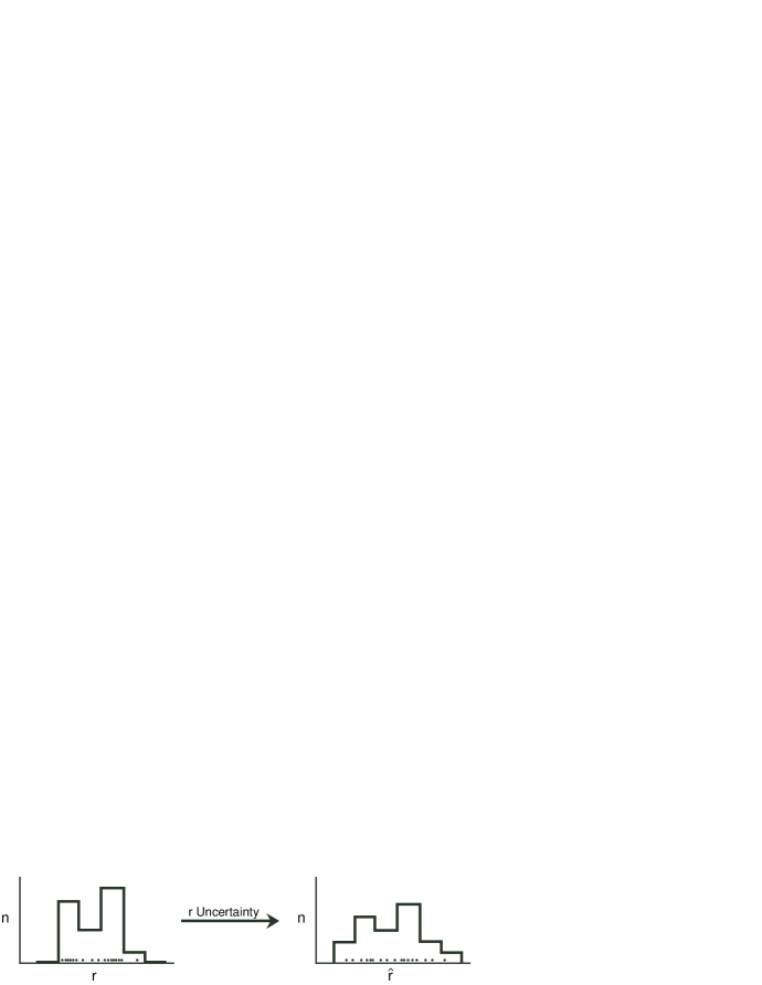
Figure 1: Distortion of the source observable distribution due to source uncertainties.

Can the distortion be removed? Jeffreys’ brief paper criticized a solution offered by Eddington that treated the problem as one of inverting a convolution; Eddington’s solution, predating understanding of the ill-posed nature of such an inversion, was highly unstable. Jeffreys pointed out that a superior approach would be to predict rather than invert the data; he suggested introducing a parameterized model and using the likelihood function to find the model parameters that best predict the data. But he did not present such a solution in any detail, and his advice was largely ignored until the 1980s.

In the meantime, Malmquist offered an approach whose basic features have guided survey analyses to this day. Rather than use the naive best-fit estimates of $r$, Malmquist showed that one could use the underlying distribution, $f(r)$, and the known size of the $\hat{r}$ uncertainties to devise corrections that lead to revised estimates, $\tilde{r}$, that can be used to estimate $f(r)$ in an unbiased manner. Malmquist’s work was so influential that biases resulting from ignoring source uncertainty have come to be known as Malmquist biases.

A serious defect of Malmquist’s approach is that the corrections depend on $f(r)$, which is unknown and often the object of interest in the investigation. Malmquist was interested in estimating the density of stars in space. He assumed that the volume density is uniform, so that the $r$ distribution is nonuniform, with $f(r)\propto r^{2}$ (due to the $r^{2}$ growth of the spherical coordinate volume element). This assumption was used for many years, but in many applications it is unsound. This is particularly the case in studies of galaxy surveys, since we know that the galaxy distribution is very nonuniform. As a result, generalizations of Malmquist’s approach have been sought. Some assume a simple parameterized form for the density (typically a power law) and determine corrections as a function of the parameter. Some procedure is then devised to set the parameter using the data, e.g., via an iterative scheme. Other approaches have an empirical Bayesian flavor (though they are typically labeled as maximum likelihood approaches); they multiply the likelihood for the $r$ value of a source by a prior determined by the source density. For a uniform density (so the prior is $\propto r^{2}$), taking $\tilde{r}$ equal to the posterior mean value of $r$ duplicates Malmquist’s corrections. Again, the density can be parameterized and the parameter adjusted using some criterion to measure consistency between the final $r$ estimates and the prior. But no rigorous, self-consistent approach has yet been offered, and research continues on how best to account for Malmquist bias.

Nothing about Jeffreys’ or Malmquist’s observations depended on the observable being distance, and the effect will be present for any other observable with a nonuniform distribution that is measured with uncertainty. Unfortunately, although the importance of correcting for such distortion is well known for space density estimation, in other applications the effect has not been so widely recognized.

The dependence of Malmquist corrections on the unknown density is a well known problem with Malmquist’s treatment of the effects of source uncertainty. But there is a more subtle potential problem that is not so widely recognized. The Malmquist approach replaces naive point estimates of observables with “corrected” point estimates. Although source uncertainties are used to determine the corrections, once the corrections are determined, the source properties are treated as precisely known in subsequent analysis. But ignoring such uncertainties can be dangerous, as the following example illustrates.

In a classic paper written in 1948 motivated by statistical problems in astronomy, Neyman and Scott Neyman and Scott (1948) discussed the following problem. For each of a number of sources we make repeated measurements of the source intensity with an instrument that adds noise to the signal. The sources each have different intensities. We assign a Gaussian distribution for the noise, but the instrument’s noise standard deviation, $\sigma$, is not known at the outset. We can pool together the data from $N$ sources to estimate the common parameter, $\sigma$ (and then use this information to estimate the source intensities).

As the simplest case, suppose there are two measurements for each object. For source $i$, the likelihood function for its intensity, $\mu_{i}$, and $\sigma$ is just the product of two Gaussians,

$${\cal L}(\mu_{i},\sigma)=\frac{1}{\sigma\sqrt{2\pi}}\exp\left[-{(x_{i}-\mu_{i})^{2}\over 2\sigma^{2}}\right]\times\frac{1}{\sigma\sqrt{2\pi}}\exp\left[-{(y_{i}-\mu_{i})^{2}\over 2\sigma^{2}}\right],$$ (1)

where $x_{i}$ and $y_{i}$ denote the two measurements. Fig. 2a shows contours of this likelihood for typical measurements with true $\sigma=1$. As one might expect, the likelihood is symmetric in $\mu_{i}$ with its peak at the sample mean, $(x_{i}+y_{i})/2$. The $\sigma$ uncertainty is large for just two measurements, but includes the true value. The dashed curve labeled “1 pair” in Fig. 2b shows a standard frequentist summary of the implications of this data for $\sigma$. The curve is the profile likelihood for $\sigma$, the maximum likelihood as a function of $\sigma$ (i.e., maximized with respect to $\mu_{i}$). Also shown is the Bayesian summary of the information in the data about $\sigma$, the marginal likelihood for $\sigma$, obtained by multiplying the likelihood by a prior for $\mu_{i}$ (here uniform) and integrating out $\mu_{i}$. (A final Bayesian inference for $\sigma$ would be found by multiplying this by a prior density for $\sigma$ to get the marginal posterior for $\sigma$.) The marginal likelihood is different from the profile likelihood, but not significantly so, given the large uncertainties.

Figure 2: The Neyman-Scott problem. (a), left, the likelihood for $\mu$ and $\sigma$ for a single pair of measurements (with measured values $x$ and $y$ shown by dots along the $\mu$ axis). Cros shows the maximum; contours are at the asymptotic 68% (dotted), 95.4% (dashed) and 99.73% (solid) confidence levels. (b), right, the profile likelihood (dashed) and marginal likelihood (solid) for $\sigma$ for a single pair, and for 20 pairs (ordinates rescaled to facilitate comparison).

Now consider what happens when we pool information from observations of 20 sources (by multiplying likelihoods). The curves labeled “20 pairs” show the results using Monte Carlo samples. The profile likelihood is converging quickly to the wrong value (it is easy to show that it asymptotically converges to $\sigma/\sqrt{2}$). The marginal distribution converges less quickly, but is peaked near the true value (and in fact is consistent—it asymptotically converges to the true value for any smooth prior). Returning to Fig. 2a, we can understand this behavior. The likelihood contours for a single pair of measurements are asymmetric in $\sigma$, enclosing much less volume in the $\mu_{i}$ direction at small values of $\sigma$ than at larger values. Focusing on the likelihood peak ignores this, leading the maximum likelihood approach astray, while accounting for the volume under the likelihood via marginalization gives correct inferences.

This problem is notable in two respects. First, it is tempting to hope that as one gathers more and more data, asymptotics comes to the rescue and guarantees convergence to the truth, with uncertainties “averaging out.” The example shows this is not true. The reason is that the the presence of source uncertainties (here in $\mu_{i}$) means that each source brings with it a new parameter that must be estimated, explicitly or implicitly. Neyman and Scott called these “incidental” parameters, in contrast to the “structural” parameter, $\sigma$, shared among all measurements. The total number of parameters present grows with the number of data so the allowed volume in parameter space does not shrink to zero asymptotically, and this feature of such problems prevents the usual asymptotic guarantees from holding.

Second, the example shows that even frequentist maximum likelihood methods, close in many respects to Bayesian methods, are insufficient in such settings. It is the Bayesian focus on volumes under likelihoods, a consequence of taking a probabilistic approach to parameter uncertainty, that leads to accurate inferences.

The Neyman-Scott problem is not merely academic. One of the problems that motivated their work frequently arises in astronomy and other disciplines: fitting data that has errors in both the abscissa and the ordinate (“errors-in-variables” models). In such problems, the unknown true abscissa values appear as nuisance parameters, and their number grows with the number of data. As a result, one must handle such problems with some care, a point made in these conferences by Ed Jaynes and Steve Gull (see Gull (1989)).

Of course, another setting where the features of Neyman’s and Scott’s problem appear is survey analysis; each source brings with it its own uncertain incidental parameters, and we learn about shared structural parameters describing the distribution of sources by pooling the information from the sources. To demonstrate the relevance of the problem to survey analysis, let us consider a concrete example.

3 Trans-Neptunian Objects

We consider surveys detecting and reporting apparent magnitudes of TNOs, a large population of minor planets with orbits extending beyond that of Neptune. The first TNOs were detected in 1992; today nearly 1000 are known. Several dynamically distinct populations comprise TNOs, distinguished by the distributions of their orbital elements. The majority are “classical” Kuiper belt objects (KBOs), with a broad distribution of low-eccentricity, low-inclination orbits. Other populations have eccentric orbits due to interactions with Neptune (“scattered” KBOs) or orbits in various resonances with Neptune (e.g., Plutinos, in orbits with a $2:3$ resonance with Neptune; Pluto is considered a member of this TNO class). We focus on classical KBOs here; see Gladman et al. Gladman et al. (2001) for a brief overview of the populations, and the review article by Luu and Jewitt Luu and Jewitt (2002), discoverers of the first TNO, for a more thorough overview. Of the $\sim 10^{3}$ known TNOs, only $\sim 10^{2}$ were discovered in surveys that have been characterized sufficiently to allow a rigorous analysis of the TNO distribution; this number will grow rapidly in the next few years. Fig. 3 presents a plan view of the solar system showing the current locations of 200 of the earliest discovered TNOs, and their relationship to the planets in the outer solar system.

Figure 3: A plan view of the outer solar system in July 2004, looking down the north ecliptic pole. The solid curves and open crosses show the orbits and locations of Jupiter, Saturn, Uranus and Neptune; $\odot$ denotes the Sun. The dashed curve and large dot show the orbit and location of Pluto, considered to be the largest of a class of TNOs called Plutinos. The small dots show the locations of 200 TNOs; about 800 have so far been discovered.

Suppose TNOs have a distribution of sizes, $D$, that is a power law, $f(D)\propto D^{-q}$, and a density distribution that varies with heliocentric radius, $r$, as a power law, $n(r)\propto r^{-\beta}$, bounded between Neptune’s orbit and some maximum distance. TNOs are seen by reflected sunlight, so the flux from a TNO obeys a $F\propto D^{2}/r^{4}$ law (ignoring for simplicity Earth’s 1 AU distance from the sun, small compared to TNO distances). The flux distribution of TNOs is then a broken power law, with the power law index of dim objects determined by $\beta$, and that of bright objects determined by $q$. Astronomers report optical fluxes on a (negative) logarithmic magnitude scale, with magnitude $m=-2.5\log_{10}F/F_{0}$ (with $F_{0}$ a fiducial flux). Let $\Sigma(m)$ be the number of TNOs per square degree with magnitudes less than $m$. The broken power law flux distribution implies a cumulative magnitude distribution that is a broken exponential,

$$\Sigma(m)=10^{\alpha(m-m_{0})},$$ (2)

where the log-slope, $\alpha$, is different at large and small $m$. For the dimmest objects (large $m$), the slope measures the TNO space density index, with $\beta=10\alpha+3$. For bright TNOs (small $m$), the slope measures the size distribution index, with $q=5\alpha+1$. Note that the parameters of physical interest, $q$ and $\beta$, are related to the more directly observable slope $\alpha$ by large factors so that small errors in $\alpha$ lead to large errors in the inferred physics. A goal of TNO survey analysis is to estimate the slope of the magnitude distribution in different magnitude ranges in order to estimate the indices of the size and density distributions.

To date well over a dozen well-characterized surveys of the TNO population have been undertaken, with extremely diverse characteristics. Some spread observing resources in relatively short exposures over broad regions of the sky along the ecliptic, providing the best data on bright TNOs (since they sample a large area). Others focus all resources on a narrow “pencil beam” target area, using repeated long exposures to search for the numerous very dim TNOs. Many surveys are unsuccessful in the sense of not detecting any new TNOs; nevertheless the lack of detections is itself useful information that sets bounds on the TNO density in the regions accessible to such surveys. Different surveys use filters that access different parts of the optical spectrum. An important challenge in TNO survey analysis is how to consistently combine the information from the many surveys.

TNOs are dim objects that are challenging to detect and measure. Measurement uncertainties due to photon counting statistics can be significant. Systematic uncertainties, e.g., due to the need to convert measurements to a common wavelength range, or due to TNO variability, can be significant. Both statistical and systematic uncertainties tend to be largest for the dimmest TNOs. For bright TNOs the magnitude uncertainty is relatively small, $\sim 5$%. For dim TNOs, it is typically much larger, 20–30%. Since distant TNOs tend to be dim, and since the volume for a given radius range is larger for distant sources than for nearby sources, many or most of the sources in a particular survey tend to be dim. Thus many of the detected TNOs have significant magnitude uncertainties. An additional challenge in TNO survey analysis is accounting for these uncertainties.

Most studies of TNO data use approaches that can be characterized as trying to “fix the data.” They try to construct a “debiased” estimate of $\Sigma(m)$ that has the selection effects of a particular survey removed. These estimates are then combined and models fitted via least squares methods. These approaches have numerous defects. The data are sparse; bins must be wide to contain enough objects to justify the asymptotic approximations underlying the methods. This sacrifices resolution; some studies simply ignore the requirement and allow bins to have few counts rather than use wide bins. The arbitrary choice of bins introduces troubling subjectivity into the results. Some studies fit the cumulative rather than differential binned distribution, ignoring the strong correlations in the binned estimates and thus seriously underestimating the uncertainty in the final inferences. None of the studies make any attempt to account for magnitude uncertainties, even though they are typically of comparable scale to the bin widths for dim sources. With such uncertainties, consistent model-independent “debiasing” is simply impossible; moreover, ignoring them risks underestimating uncertainties in the final inferences, and possibly finding incorrect results due to the volume effects discussed above.

Bayesian inference is ideally suited to the challenges of TNO survey analysis. Information from disparate surveys can be easily combined by multiplying likelihoods. Source uncertainties can be handled by introducing nuisance parameters and marginalizing. Systematic error can be incorporated in the analysis, since the Bayesian approach does not restrict use of probability distributions only to “random” uncertainties.

Gladman et al. Gladman et al. (1998, 2001) have adopted a Bayesian approach to TNO survey analysis, building on the work of Loredo and Wasserman on analysis of GRB survey data Loredo and Wasserman (1995, 1998a, 1998b). Their results differ markedly from those of investigators using the approaches described above. More recently, Bernstein et al. (Bernstein (2004); B04) have advocated a quasi-Bayesian approach, but with an incorrect likelihood function. In the remainder of this section, I will describe the Bayesian approach and how it differs from the B04 approach, illustrating how some of the concerns of the previous section can manifest themselves in analyses of TNO survey data. The results show that it is not enough to follow the Bayesian approach “in spirit;” inferences can be significantly corrupted unless the Bayesian prescription is followed with care.

For an analysis of the TNO magnitude distribution, the information from a TNO survey can be summarized by reporting the following quantities:

• The solid angle, $\omega$, examined by the survey;

• The survey efficiency function, $\eta(m)$, specifying the probability that a TNO of magnitude $m$ will produce data meeting the survey criteria for detection;

• Source likelihood functions, $\ell_{i}(m)$, giving the likelihood that TNO $i$ has magnitude $m$. By definition $\ell_{i}(m)=p(d_{i}|m,M)$ is the probability for the data $d_{i}$ from source $i$ presuming the source has magnitude $m$, with $M$ denoting any data modeling assumptions. It will often be adequately summarized by a Gaussian function specified by the best-fit (maximum likelihood) $m$ value for the TNO and its uncertainty.

Our goal here is to infer the parameters, $\theta$, of a specified model for the TNO magnitude distribution. The key ingredient in a Bayesian analysis is the likelihood function for $\theta$ based on all the survey data, $D$, defined by ${\cal L}(\theta)=p(D|\theta,M)$. We will derive it in two steps. First, we derive the likelihood for an idealized survey able to detect every TNO brighter than some magnitude, $m_{\rm th}$, and reporting the magnitude of TNO $i$ precisely as $m_{i}$. Then we account for the complications of detection efficiency and source uncertainty.

We model the magnitude distribution as a Poisson point process specified by the differential magnitude distribution, $\sigma(m)$, defined so that $\sigma(m)dmd\omega$ is the probability for there being a TNO of magnitude in $[m,m+dm]$ in a small patch of the sky of solid angle $d\omega$ (so $\Sigma(m)$ is its integral). For idealized data, we imagine the $m_{i}$ values spread out on the magnitude axis, shown in Fig. 4. We divide the axis into empty intervals indexed by $\alpha$ with sizes $\Delta_{\alpha}$, between small intervals of size $\delta m$ containing the $N$ detected values $m_{i}$. The expected number of TNOs in empty interval $\alpha$ is,

$$\mu_{\alpha}=\omega\int_{\Delta_{\alpha}}dm\;\sigma(m).$$ (3)

The expected number in the interval $\delta m$ associated with detected TNO $i$ is

$$\mu_{i}=\omega\,\delta m\,\sigma(m),$$ (4)

where we take $\delta m$ small enough so the integral over $\delta m$ is well approximated by this product. The probability for seeing no TNOs in empty interval $\alpha$ is the Poisson probability for no events when $\mu_{\alpha}$ are expected, given by $e^{-\mu_{\alpha}}$. The probability for seeing a TNO of magnitude $m_{i}$ in $\delta m$ is the Poisson probability for one event when $\mu_{i}$ are expected, given by $\mu_{i}e^{-\mu_{i}}$. Multiplying these probabilities gives the likelihood for the parameters, $\theta$, specifying $\sigma(m)$. The expected values in the exponents sum to give the integral of $\sigma(m)$ over all accessible $m$ values, so the likelihood can be written,

$${\cal L}(\theta)=(\omega\delta m)^{N}\exp\left[-\omega\int dm\,\Theta(m_{\rm th}-m)\sigma(m)\right]\prod_{i=1}^{N}\sigma(m_{i}),$$ (5)

where $\Theta(m_{\rm th}-m)$ is a Heaviside function restricting the integral to $m$ values smaller than $m_{\rm th}$. The factor in front is a constant that will drop out of Bayes’s theorem and can henceforth be ignored.

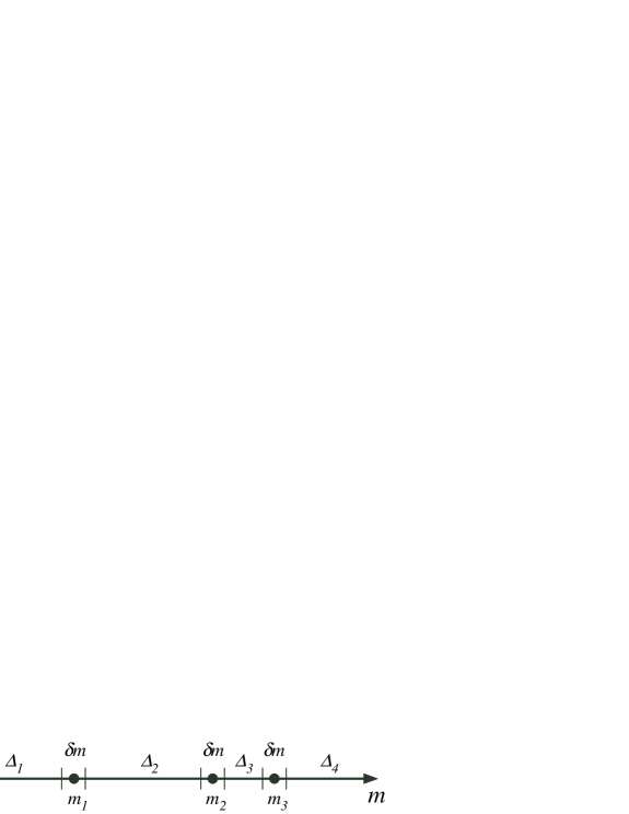
Figure 4: Constructing the likelihood for an idealized survey as a point process in $m$, with empty intervals of sizes $\Delta_{\alpha}$ and TNOs detected at points $m_{i}$ in small intervals of size $\delta m$.

Now we consider the real survey data, which differs from the idealized data in two ways: the presence of a survey efficiency rather than a sharp threshold, and the presence of magnitude uncertainties. We immediately run into difficulty with a point process model because we cannot make the construction of Fig. 4, since we do not know the precise values of the TNO magnitudes. But in a Bayesian calculation we can introduce these values as nuisance parameters, and then integrate them out. To facilitate the calculation, we need to introduce some notation. When occurring as an argument in a probability, let $m_{i}$ denote the proposition that there is a TNO of magnitude $m_{i}$ in an interval $\delta m$ at $m_{i}$. We divide the data, $D$, into two parts: the data from the detected objects, $\{d_{i}\}$, and the proposition, ${\cal N}$, asserting that no other objects were detected. Then the likelihood can be written,

$${\cal L}(\theta) = p(D|\theta,M)$$ (6)

$$= \int\{dm_{i}\}\;p(\{m_{i}\},{\cal N}|\theta,M)\,p(\{d_{i}\}|\{m_{i}\},{\cal N},\theta,M).$$

The first factor in the integrand can be calculated using a construction similar to that used for the idealized likelihood above, with one important difference: the presence of the ${\cal N}$ proposition means that we cannot assume that no TNO is present in a $\Delta_{\alpha}$ interval, but rather that no TNO was detected. Thus these probabilities are Poisson probabilities for no events when $\mu_{\alpha}$ are expected, with

$$\mu_{\alpha}=\omega\int dm\;\eta(m)\,\sigma(m),$$ (7)

the detectable number of TNOs in the interval rather than the total number. Thus the first factor in the integrand in equation (6) resembles the right hand side of equation (5), but with $\eta(m)$ replacing the Heaviside function in the integral in the exponent.

The second factor in the integrand in equation (6) is the probability for the data from the detected objects, given their magnitudes. Since the source likelihood function is by definition $\ell_{i}(m)=p(d_{i}|m)$, this probability is just a product of source likelihood functions evaluated at the specified $m_{i}$ values (with the $m_{i}$ values given, the ${\cal N}$ and $\theta$ propositions in this probability are irrelevant to the probability for $d_{i}$). Now we can calculate equation (6):

$${\cal L}=\exp\left[-\omega\int dm\,\eta(m)\sigma(m)\right]\prod_{i}\int dm\,\ell_{i}(m)\sigma(m),$$ (8)

where we have dropped the unimportant interval factors, and we have simplified the notation by dropping the indices from the $m_{i}$ variables in the integrals, since they are just integration variables for independent integrals.

B04 derived a likelihood function for TNO magnitude data by an informal argument, with their final result being,

$${\cal L}_{B}=\exp\left[-\omega\int dm\,\eta(m)\sigma(m)\right]\prod_{i}\int dm\,\eta(m)\ell_{i}(m)\sigma(m).$$ (9)

This differs from equation (8) in the presence of $\eta(m)$ factors in the source integrals. B04 argued that these factors should be present because the probability for the data from a detected TNO with given magnitude should be the product of the probability that the TNO was detected, given by $\eta(m)$, times the probability for the detection data. But this is an incorrect calculation of a joint probability. Let ${\cal D}_{i}$ denote the proposition that a TNO is actually detected in the data from TNO candidate $i$. The product rule lets us calculate the joint probability for ${\cal D}_{i}$ and $d_{i}$ in two ways:

$$p({\cal D}_{i},d_{i}|m,M) = p(d_{i}|m,M)p({\cal D}_{i}|d_{i},m,M)$$ (10)

$$= p({\cal D}_{i}|m,M)p(d_{i}|{\cal D}_{i},m,M).$$

In the first line, the first factor is just the source likelihood, $\ell_{i}(m)$. The second factor is the probability that TNO $i$ is detected, given the data from that TNO. But since we are considering data from a detected TNO, this probability is unity by definition (i.e., detection is a criterion that the observed data are in some acceptable set, and by definition data from a detected TNO must lie in that acceptable set). So the joint probability for detection and the data, given $m$, is just the isolated $\ell_{i}(m)$ term appearing in the correct likelihood.

Now examine the second line in equation (10), corresponding to the factorization implicitly used by B04. The first factor is the probability that a TNO of magnitude $m$ would be detected; this is given by $\eta(m)$. But the second term is the probability for the data from the detected TNO, given that it has been detected. We can calculate this probability with Bayes’s theorem; it is given by $\ell_{i}(m)/\eta(m)$. The $\eta$ factors cancel, and this factorization of the joint probability also equals $\ell_{i}(m)$, as it must. The B04 derivation fails to condition on detection when calculating the data probability, and so produces an incorrect final likelihood function.

To make these considerations concrete, imagine a simple detector that counts photons in a single pixel, and reports a detection if the counts exceed some threshold, $n_{\rm th}$. The data from detected source $i$ is just the counts, $n_{i}$, detected from that source. Then the first factorization is the product of the Poisson probability for $n_{i}$ counts given the magnitude, and the probability that $n_{i}>n_{\rm th}$. Since the source was detected, the last probability is unity, and we are left with the Poisson likelihood for $m$ defining $\ell_{i}(m)$. For the second factorization, the first factor is the probability that $n_{i}>n_{\rm th}$ given the TNO magnitude. This is a sum of Poisson probabilities for counts above $n_{\rm th}$ (it is given by an incomplete Gamma function). The second factor is the probability for seeing $n_{i}$ counts from a source of magnitude $m$, given that the counts from that source are above $n_{\rm th}$. This is the Poisson probability for $n_{i}$, but renormalized for counts above the threshold. The renormalization requires division by the sum given by the first factor, so that factor cancels and again we are left with the Poisson probability for $n_{i}$ counts given $m$, that is, $\ell_{i}(m)$ (with no $\eta(m)$ factor).

B04 further argued that the uncertainties were small enough that they could be ignored, essentially taking $\ell_{i}(m)$ to be a $\delta$-function at the best-fit magnitude, $\hat{m}_{i}$. In this approximation the integral for object $i$ becomes $\eta(\hat{m}_{i})\sigma(\hat{m}_{i})$. The first factor is constant with respect to the model parameters, so this corresponds to a likelihood function given by,

$${\cal L}^{\prime}_{B}=\exp\left[-\omega\int dm\,\eta(m)\sigma(m)\right]\prod_{i}\sigma(\hat{m}_{i}).$$ (11)

This is the idealized likelihood of equation (5), with the Heaviside function replaced by the detection efficiency. This is the likelihood actually used by B04.

To explore the consequences of use of the incorrect likelihood of equation (9), and of completely ignoring uncertainty and using equation (11), we can construct simple simulated surveys where the truth is known and see if these likelihoods recover the truth. I simulated data from a TNO distribution with a “rolling” power law index using a model advocated by B04,

$$\sigma(m)=\sigma_{23}10^{[\alpha(m-23)+\alpha^{\prime}(m-23)^{2}]},$$ (12)

where $\sigma_{23}$ is the density at $m=23$, $\alpha$ is the power law slope at $m=23$, and $\alpha^{\prime}$ is the rate of change of the slope with $m$. TNO magnitudes were drawn from this distribution, and then the counts expected from that source in a simple single-pixel measurement were sampled from a Poisson distribution with expected value proportional to the flux. If the counts were above a threshold, $n_{\rm th}$, the TNO was detected, and its Poisson likelihood was used for $\ell(m)$. For the results shown in Fig. 5, the threshold and expected counts were chosen so that the dimmest detected TNOs had an uncertainty $\sim 33$%. The model used has $\alpha=0.75$ and $\alpha^{\prime}=-0.05$, a model B04 find describes classical KBOs well. Fig. 5a shows the most probable parameter values from 100 simulated surveys with $N=100$ detected TNOs; the values were found by calculating the marginal distribution for $\alpha$ and $\alpha^{\prime}$ using flat priors. The solid dots show estimates using the correct likelihood; the open circles show estimates ignoring source uncertainty, using equation (11). Estimates from the correct likelihood are scattered roughly symmetrically about the true value (indicated by the open $\times$). Estimates ignoring source uncertainties systematically overestimate $\alpha$ and underestimate $\alpha^{\prime}$. For samples of this size (comparable to the size of the sample analyzed by B04), the uncertainties are large enough that the estimates are still sometimes near the correct value despite the strong bias. Fig. 5b shows estimates with $N=1000$, and the situation is worse—-the estimates ignoring uncertainty are converging away from the truth, similar to the behavior seen in the Neyman-Scott problem. In contrast, the correct likelihood produces estimates converging on the true value. Figs. 5c,d repeat the experiment using the likelihood of equation (9) that attempts to include uncertainties, but has the incorrect $\eta(m)$ factor. We find the same behavior, indicating that even though equation (9) has integrals over the source uncertainties, the incorrect $\eta(m)$ factors corrupt inferences using this likelihood.

Figure 5: Parameter estimates from analyses of simulated data from a rolling power law model, using the correct (solid dots) and incorrect (open dots) TNO survey likelihood. Open “$\times$” indicates the true parameter values. (a,b) Estimates using a likelihood that ignores parameter uncertainties, for TNO samples of size 100 (a) and 1000 (b). (c,d) Estimates using a likelihood with incorrect source uncertainty integrals, for TNO samples of size 100 (c) and 1000 (d).

These simulations do not necessarily call into question the final scientific findings reported by B04. The simulations used a simplified survey protocol, with somewhat larger magnitude uncertainties than B04 claim for their data, and in any case indicate that for samples with similar size to that studied by B04, correct results are sometimes found by chance. What the simulations do indicate is that use of the incorrect likelihood will eventually lead to trouble as sample sizes get larger.

The principle lesson of this work is that source uncertainties must be carefully accounted for in analyses of survey data. In particular, the effects of source uncertainties do not “average out” as data sets grow in size, but in fact can grow more severe. Bayesian inference proves to be an ideal tool for handling this problem. By accounting for volumes in parameter space—especially volumes associated with incidental parameters that arise due to source uncertainties—a Bayesian analysis can accurately account for the distortions introduced by source uncertainties. Further work on this issue, including a more thorough examination of the B04 results, will be reported elsewhere.

References

- Jeffreys (1938) Jeffreys, H., Mon. Not. Roy. Ast. Soc., 98, 190 (1938).
- Neyman and Scott (1948) Neyman, J., and Scott, E. L., Econometrica, 16, 132 (1948).
- Gull (1989) Gull, S., “Bayesian Data Analysis—Straight Line Fitting,” in Maximum Entropy and Bayesian Methods, edited by J. Skilling, Kluwer, Dordrecht, 1989, pp. 511–518.
- Gladman et al. (2001) Gladman, B., Kavelaars, J. J., Petit, J., Morbidelli, A., Holman, M. J., and Loredo, T., Astron. J., 122, 1051–1066 (2001).
- Luu and Jewitt (2002) Luu, J. X., and Jewitt, D. C., An. Rev. Astron. Astrophys., 40, 63–101 (2002).
- Gladman et al. (1998) Gladman, B., Kavelaars, J. J., Nicholson, P. D., Loredo, T. J., and Burns, J. A., Astron. J., 116, 2042–2054 (1998).
- Loredo and Wasserman (1995) Loredo, T. J., and Wasserman, I. M., Astrophys. J. Supp., 96, 261–301 (1995).
- Loredo and Wasserman (1998a) Loredo, T. J., and Wasserman, I. M., Astrophys. J., 502, 75 (1998a).
- Loredo and Wasserman (1998b) Loredo, T. J., and Wasserman, I. M., Astrophys. J., 502, 108 (1998b).
- Bernstein (2004) Bernstein, G., et al., Astron. J., in press, astro–ph/0308467 (2004).
- Loredo and Lamb (1989) Loredo, T. J., and Lamb, D. Q., Ann. N. Y. Acad. Sci., 571, 601–630 (1989).
- Loredo and Lamb (2002) Loredo, T. J., and Lamb, D. Q., Phys. Rev. D, 65, 063002 (2002).