DASI Three-Year Cosmic Microwave Background Polarization Results

Abstract

We present the analysis of the complete 3-year data set obtained with the Degree Angular Scale Interferometer (DASI) polarization experiment, operating from the Amundsen-Scott South Pole research station. Additional data obtained at the end of the 2002 Austral winter and throughout the 2003 season were added to the data from which the first detection of polarization of the cosmic microwave background radiation was reported. The analysis of the combined data supports, with increased statistical power, all of the conclusions drawn from the initial data set. In particular, the detection of $E$-mode polarization is increased to $6.3\sigma$ confidence level, $\it TE$ cross-polarization is detected at $2.9\sigma$, and $B$-mode polarization is consistent with zero, with an upper limit well below the level of the detected $E$-mode polarization. The results are in excellent agreement with the predictions of the cosmological model that has emerged from CMB temperature measurements. The analysis also demonstrates that contamination of the data by known sources of foreground emission is insignificant.

1 Introduction

The use of the cosmic microwave background (CMB) as a precision probe of the composition and dynamics of the universe presumes the correctness of the theoretical framework by which we understand its origin and evolution. With the detections of CMB polarization anisotropy by DASI (Kovac et al., 2002, hereafter Paper V) and WMAP (Kogut et al., 2003) that framework itself has passed a critical test, as the presence of polarization is a generic requirement of the physics of recombination (for a recent review see Hu & Dodelson, 2002). The intrinsic polarization of the CMB reflects the local radiation field anisotropy, specifically the quadrupole moment, at the surface of last scattering, 14 billion years ago. Within the context of the standard cosmological model, in which peaks in the CMB angular power spectrum are interpreted as the signature of acoustic oscillations seeded by primordial density fluctuations, current temperature measurements lead to specific predictions for the shape and amplitude of the polarization power spectrum and the temperature-polarization cross power spectrum. Furthermore, it is a firm prediction that density fluctuations should create only $E$-mode, i.e., curl-free, polarization patterns on the sky.

In Paper V, we reported the high signal to noise (s/n) detection of $E$-mode polarization in the CMB with DASI. Kogut et al. (2003) reported the detection of the $\it TE$ correlation on larger angular scales by WMAP. The DASI and WMAP measurements underscore the power of combining sub-orbital experiments, with their ability to achieve exquisite sensitivity over small areas of sky, with space experiments, whose sky coverage allows them to approach fundamental sample variance limits. These measurements provide fuel for a host of new experiments aimed at probing the detailed polarization spectrum of the CMB, from the largest scales, which may bear the signature of inflationary gravitational waves, to the smallest, where the CMB is expected to record the history of structure formation.

In Paper V, we presented the analysis of the initial DASI polarization data set obtained during 2001 and the first part of the 2002 season; modifications to the instrument to enable polarization measurements, as well as the observations and calibration of the data, were described in Leitch et al. (2002a, hereafter Paper IV). In this paper we present the analysis of the 3-year DASI polarization data set, which comprises the initial data (271 days of observations) and the additional data collected during the end of the 2002 season and over the entire 2003 season (191 days in all). The end of the 2003 season marked the conclusion of interferometric observations with DASI.

2 Observations

2.1 Instrument Review

The use of interferometers, and of DASI in particular, to measure the angular power spectrum of CMB anisotropy is described extensively in Leitch et al. (2002b, hereafter Paper I) and in Paper IV. In short, an interferometer detects correlations between pairs of antennas, i.e., baselines, yielding measurements which are largely insensitive to uncorrelated noise, and which map simply into Fourier components of the sky brightness distribution, longer baselines measuring higher spatial frequencies. As they operate natively in the Fourier plane, interferometers are ideally suited to measurement of the power spectrum.

DASI is a 13-element, co-planar interferometric array operating in ten 1-GHz bands spanning $26-36~{}$GHz. The telescope sits atop an eleven meter tower located at the Amundsen-Scott South Pole research station. DASI was initially configured for measurements of the CMB temperature anisotropy on angular scales corresponding to multipoles $140<l<900$ (Paper I). These observations were completed during the 2000 Austral winter and the results reported in Halverson et al. (2002, hereafter Paper II) and Pryke et al. (2002, hereafter Paper III). As described in Paper IV, several changes were made for the polarization observations, including the installation of a large reflective radiation shield surrounding the telescope. The shield geometry ensures that all lines of sight from the telescope in the direction of the station buildings, the horizon and ground, are reflected to the sky. To provide polarization sensitivity, the thirteen DASI receivers were each equipped with cooled, broadband achromatic polarizers which can be mechanically set to accept either left or right-circularly polarized light. Within each 1-hour interval of observation, the polarizers were stepped between right ($R$) and left ($L$) positions to acquire data in all four Stokes states, which we refer to as co-polar ($\it RR$, $\it LL$) and cross-polar ($\it RL$, $\it LR$) data.

A sun shield, designed to extend the polar observing season to include periods just before sunset and after sunrise, was installed for the 2002 season. The shield was found to contaminate the shortest baselines by secondary reflection at times when the moon was above the horizon, and was removed for the final season. (Note however that the large ground shield remained in place during all three seasons.) Apart from the installation and removal of the sun shield, and replacement of miscellaneous hardware during routine maintenance of the telescope, the instrument was identical throughout the three seasons discussed here.

2.2 Observing Strategy

The polarization experiment consisted of deep observations of two $3\fdg 4$ FWHM fields, at Right Ascension 23^h30^m and 00^h30^m, and Declination $-55^{\circ}$ (J2000) (see Figure 1). Details of the field selection are given in Paper IV. The fields were observed continuously at constant elevation (one of the unique advantages of observing from the South Pole), interspersed with daily observations of a calibrator source. A variety of cross-checks were built into the experiment design. Observations of the two fields were interleaved on 1-hour timescales to ensure that each was observed over the same azimuth range, allowing effective removal of any residual ground signals by differencing the data. The configuration of the array elements is threefold symmetric and the entire array is fixed to a faceplate which can be rotated along the line of sight. On 24-hour timescales, the observations alternated between two different orientations of the faceplate, offset by 60^∘, in which the same Fourier components are measured, but by different pairs of antennas.

Throughout the three seasons of observations, the observing strategy, as described in Paper IV, remained identical.

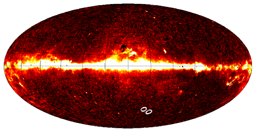
Figure 1: Polarization field locations. DASI fields are marked by white circles, plotted over the Ka-band synchrotron map derived from the WMAP first-year data (Bennett et al., 2003). The color scale is linear and has been clipped at one thirtieth of the maximum to allow the structure at high Galactic latitudes to be seen.

2.3 Data Cuts

A variety of cuts, discussed extensively in Paper IV, are applied to the data before input to the likelihood analyses; cut criteria and thresholds for the combined three-season data were the same as for the data presented in Paper IV and Paper V. During the 2002 season, when it was discovered that the short-baseline data were affected by reflections of the moon off the sun shield, a more stringent cut on the elevation of the moon was applied than during the 2001 season. During the 2003 season, for which the sun shield had been removed, cuts on the moon were relaxed to the 2001 levels. Early in the 2003 season, the polarizer assembly for one of the DASI receivers began to slip, and data associated with this receiver were therefore excised for the entire season, removing $\sim 15\%$ of the 2003 data.

Of the three-season data taken with the sun below the horizon, approximately $53\%$ of the co-polar data, and $61\%$ of the cross-polar data passed the data cuts. Cut fractions were dominated by cuts on the elevation of the moon, and by cuts on the complex gains of multipliers in the correlator (see Paper IV).

2.4 Calibration

The instrumental response of each baseline of an interferometer is the complex multiplication of the individual antenna responses. As a result, the polarization calibration, up to an absolute phase offset, can be derived from observations of an unpolarized source (see Paper IV). The remaining phase offset was determined by observing an unpolarized source through linearly polarizing wire grids attached to the front of each receiver. These offsets had previously been measured in 2001 August and 2002 February. The wire-grid calibrations were performed again in 2003 March and 2003 October, and results from all four epochs agree to within the measurement uncertainties.

Leakage from one polarization state to the other will mix CMB power from $T$ into $E$-modes and $B$-modes, and must be included in the analysis. Ideally these should be kept as small as possible, but even significant leakages can be accounted for if they are stable. The leakages can be separated into a component due to the polarizers (referred to as on-axis leakages in Paper IV), and a beam-dependent component which derives from the inherent properties of the optics (referred to as off-axis leakages in Paper IV). The latter were characterized in Paper IV, and are not expected to change. The on-axis leakages for DASI were determined from observations of a bright unpolarized source in 2001 August, 2002 April, 2002 July and 2003 August. On-axis leakages of total intensity into the cross-polarized data were found to be less than $1\%$ at all but the highest frequency bands (see Paper IV) and were consistent from year to year.

3 Results

3.1 Noise Model and Consistency Tests

For both the $\chi^{2}$ consistency tests and likelihood analyses that follow, the calibrated, field-differenced, and co-added visibility data are arranged in a data vector that is considered to be the sum of signal and noise components, $\mathbf{\Delta}=\mathbf{s}+\mathbf{n}$. An accurate characterization of the instrument noise in the data vector is critical for estimating the faint polarization signal. We calculate various statistics from the raw data to test our assumptions about the noise model: namely, that the noise is Gaussian, that the noise variance is well approximated by the variance in the 8.4-s samples (the fundamental data rate) over 1-hr intervals before field differencing, and that the noise is uncorrelated between data vector elements.

Details of the noise model tests and results for the initial data set are given in Paper V. We find similar results for the 3-year data. Three different types of short-timescale (1-hr) variance estimators are in excellent agreement with one another, and also with the variance derived from the scatter of 1-hr binned visibilities over the 3-year span of the data set. In Paper V, we scaled the noise by a factor of 1% (twice the maximum discrepancy among the various noise estimators described above) to test the robustness of our noise estimate and found no significant change in the likelihood results.

We construct a data covariance matrix for each day of observation to test the assumption that the noise covariance matrix is diagonal, and to form a cut statistic based on correlated atmospheric noise. Data covariance matrices for all good-weather days are averaged, to test for noise correlations persistent throughout the data set. We find significant correlations in 0.017% of the off-diagonal terms. These are similar in number and magnitude to those previously described in Paper V, where we found that adding the measured correlations to the noise model had a negligible effect on the final results.

We construct a $\chi^{2}$ statistic on sum and difference data vectors for various splits and subsets of the data in which the same signal is expected, as a simple but powerful test of the noise model, data consistency, and presence of signal in the data. The statistic is given by $\chi^{2}=\mathbf{\Delta}^{t}\mathbf{C}_{N}^{-1}\mathbf{\Delta}$, where $\mathbf{\Delta}=\left(\mathbf{\Delta_{1}}\pm\mathbf{\Delta_{2}}\right)/2$ is the sum or difference data vector, and $\mathbf{C}_{N}=\left(\mathbf{C}_{N1}+\mathbf{C}_{N2}\right)/4$ is the corresponding noise covariance matrix. We assess the significance of a $\chi^{2}$ value by calculating the probability to exceed (PTE) that value in the cumulative distribution function.

Following the procedure in Paper V, we split the data by epoch, azimuth range, faceplate position, and Stokes state (for co-polar observations) for each of the three years of data individually, for each year versus the other two, and for the full 3-year dataset. For each split, we also examine various subsets of the data vector, including co-polar and cross-polar data, data in distinct multipole ranges and the high expected s/n eigenmodes. In all, over 400 $\chi^{2}$ tests were performed on various splits/subsets of the data.

The distribution of $\chi^{2}$ values for the differenced polarization data shows no evidence for residual signal in excess of the noise, giving a uniform distribution of PTE values with no apparent trends or outliers. In the 2003 temperature data, several subsets which isolate high expected s/n eigenmodes formed from the shortest baselines compared at different faceplate rotations yield high $\chi^{2}$ values, the most significant of which gives a PTE = 0.0004. Because this discrepancy appears in an isolated subset of data which contains an extremely high signal, it is suggestive of a small shift in instrumental response. Such a shift at the level suggested by these tests would not significantly affect the data.

For the sum data vectors, a signal is detected with high significance in all of the co-polar splits and subsets, as well as in many of the high s/n subsets of the cross-polar data. In addition to the split data tests, we construct $\chi^{2}$ statistics from the highest s/n eigenmodes of the unsplit data vectors, as a sensitive check for the presence of signal, as discussed in Paper V. In the cross-polar data, the number of expected s/n $>1$ polarization eigenmodes has increased from 34 in the initial data set to 60 for the 3-year data set (taking into account off-axis leakage terms in the noise covariance matrix $\mathbf{C}_{N}$, see Paper V). For these eigenmodes, we find $\chi^{2}=141.3$, which corresponds to a PTE of $1.66\times 10^{-8}$ — a high-significance detection of a polarized signal.

The results of both the $\chi^{2}$ consistency tests and the noise model tests demonstrate that the noise is well characterized and Gaussian, and that the data calibration is consistent over the three years of observations. The sum data vector $\chi^{2}$ tests on both the co-polar and cross-polar data indicate the detection of signal with high-significance, using a simple test that is independent of the more sophisticated likelihood analysis results that follow.

3.2 Systematic uncertainties

In Paper V, we investigated the impact of possible sources of systematic uncertainties on the results of the likelihood analysis. In addition to the uncertainties in the noise model discussed above, we considered systematic uncertainties in the absolute cross-polar phase offsets, in the on-axis and off-axis leakages (see §2.4 for definitions), and in the pointing of the telescope. In each case, re-analyzing the data with the systematic errors set to the limits of their allowed ranges led to insignificant shifts in the results.

The overall uncertainty of the DASI absolute calibration, derived from measurements of external thermal loads, transferred to an astronomical calibrator, was estimated in Paper II to be 8% (1$\sigma$), expressed as a fractional uncertainty on the $C_{l}$ bandpower (4% in $\Delta T/T$), and applies equally to the temperature and polarization data.

3.3 Likelihood Results

The same likelihood analysis formalism described in Paper V was used to analyze the DASI 3-year polarization data set. We place constraints on a given set of parameters by characterizing the shape of the likelihood function, i.e., the probability of our data vector $\mathbf{\Delta}$, given a set of parameters $\mathbf{\kappa}$ which describe the signal,

$$L\left(\mathbf{\kappa}\right) = P\left(\mathbf{\Delta}|\mathbf{\kappa}\right)$$ (1)

$$\propto \det\left(\mathbf{C}\left(\mathbf{\kappa}\right)\right)^{-1/2}\exp\left(-\frac{1}{2}\mathbf{\Delta}^{t}\mathbf{C}\left(\mathbf{\kappa}\right)^{-1}\mathbf{\Delta}\right),$$

where $\mathbf{C}\left(\mathbf{\kappa}\right)$ is a model for the covariance matrix of the data vector. This matrix contains the expected contributions of the instrument noise and the cosmological signal, as seen through the particular filter of the experiment. Details of the construction of $\mathbf{C}\left(\mathbf{\kappa}\right)$ for the DASI polarization data set are given in Paper V and in Kovac (2003).

We report the maximum likelihood (ML) values of the parameters $\mathbf{\kappa}$, found using an iterated quadratic estimator technique (Bond et al., 1998). The shape of the likelihood function in the vicinity of the ML peak is characterized using direct grid evaluation for those analyses with four or fewer parameters, and using a Markov chain algorithm for higher dimensional analyses (Christensen et al., 2001). Confidence intervals for individual parameters are obtained by marginalizing (integrating) the likelihood function over the remaining parameters, and reporting the equal-likelihood bounds which enclose 68% of the marginal likelihood distribution (the so-called highest posterior density (HPD) interval). These are given in the text in the format: ML (HPD-low to HPD-high). For parameters which are intrinsically positive, we consider placing (physical) upper limits by marginalizing the likelihood distribution as before, but excluding the unphysical negative values. We then test if the 95% integral point has a likelihood smaller than that at zero; if it does, we report an upper limit rather than a confidence interval. We also include in tabulated results the uncertainty estimates and parameter correlation coefficients obtained by evaluating the Fisher curvature matrix $F$ at the peak of the likelihood function.

Our goodness-of-fit statistic, as described in Paper V, is the logarithmic ratio of the maximum of the likelihood to its value for some hypothetical model ${\cal H}_{0}$ described by parameters $\kappa_{0}$,

$$\Lambda({\cal H}_{0})\equiv-\log\left(\frac{L\left(\kappa_{ML}\right)}{L\left(\kappa_{0}\right)}\right)\,.$$

In the limit where the $\kappa_{ML}$ parameter uncertainties are normally distributed, the statistic reduces to $\Lambda=\Delta\chi^{2}/2$. Where possible, we have tested the distribution of $\Lambda$ using Monte Carlo simulations and found $\Delta\chi^{2}/2$ to be an excellent approximation. We therefore use the well-known $\chi^{2}$ cumulative distribution function to compute the probability that, assuming a given hypothetical model ${\cal H}_{0}$ to be true, we would obtain a value for $\Lambda({\cal H}_{0})$ that exceeds the observed value. This is quoted in the text and tabulated results as a PTE and, where appropriate, as a significance of detection, in units of $\sigma$.

For the 3-year data set, we perform all of the analyses reported in Paper V for the initial data set. In addition, we perform two new analyses to constrain the level of contamination from synchrotron or radio point source emission. The separate likelihood analyses constrain different aspects of the signal in the polarization data, in the temperature data, or in both analyzed together. The numerical results are given in Tables 1, 2 and 3, respectively. Closely following the format from Paper V, we now briefly discuss each analysis in turn.

3.3.1 $E/B$ Analysis

In this analysis, two single-bandpower parameters are used to characterize the amplitudes of the $E$ and $B$ polarization spectra. DASI has an instrumental response to $E$ and $B$ that is symmetric and nearly independent. Although the B spectrum is not expected to have the same shape as the $E$ spectrum, we choose the same shape for both spectra to preserve this symmetry in the analysis.

Following Paper V, we consider three a priori shapes to determine which is most favored by the data: the concordance $E$ spectrum shape, and two alternatives: a flat $l(l+1)C_{l}\propto\rm{constant}$ spectrum, and a power law $l(l+1)C_{l}\propto l^{2}$ spectrum. For each of these three cases, the point at $E=0,\ B=0$ corresponds to the same zero-polarization nopol model, so that the likelihood ratios $\Lambda({\it nopol})$ may be compared directly to assess the relative likelihoods of the best-fit models. For the flat case, the ML flat bandpower values are $E=6.2\mu K^{2},B=0.0\mu K^{2}$, with $\Lambda({\it nopol})=10.58$. For the $l^{2}$ power law case, the ML values are $E=4.2\mu K^{2},B=0.0\mu K^{2}$ ($l(l+1)C_{l}/2\pi$ at $l=300$), with $\Lambda({\it nopol})=15.41$. For the concordance shape, the ML values are $E=0.73,B=0.03$ in units of the concordance $E$ spectrum amplitude, with $\Lambda({\it nopol})=20.10$. Although each of these analyses shows strong evidence for an $E$ polarization signal, the likelihood of the best fit model in the concordance case is a factor of 110 and 14,000 higher than those of the $l^{2}$ power law and flat cases, respectively. The data clearly prefer the concordance shape, which we therefore use for the $E/B$ and other single bandpower analyses.

Figure 2 illustrates the result of the $E/B$ concordance-shape polarization analysis. The maximum likelihood value of $E$ is 0.73 (0.53 to 0.95 at 68% confidence). For $B$, the result should clearly be regarded as an upper limit; 95% of the $B>0$ likelihood (marginalized over $E$) lies below 0.25.

The data are highly incompatible with the no polarization hypothesis. The likelihood ratio $\Lambda({\it nopol})=20.10$ implies a probability that the data are consistent with the zero polarization hypothesis of $\rm{PTE}=1.86\times 10^{-9}$, assuming that the uncertainties in $E$ and $B$ are normally distributed, as discussed above. Marginalizing over $B$, we find $\Lambda(E=0)=19.65$, corresponding to detection of $E$-mode polarization at a PTE of $3.64\times 10^{-10}$, or a significance of $6.27\sigma$.

The likelihood ratio for the concordance model gives $\Lambda(E=1,\,B=0)=0.68$, for which the PTE is 0.51. We conclude that the data are consistent with the concordance model.

Figure 2: Results from the two-parameter shaped bandpower $E/B$ polarization analysis. We assume the $E$-mode power spectrum shape predicted for the concordance model, and the units of amplitude are relative to that model. The same shape is assumed for the $B$-mode spectrum. (right panel) The point shows the maximum likelihood value with the cross indicating Fisher matrix errors. Likelihood contours are placed at levels $\exp(-n^{2}/2)$, $n=1,2...$, relative to the maximum, i.e., for a normal distribution, the extrema of these contours along either dimension would give the marginalized $n$-sigma interval. (left panels) The corresponding single-parameter likelihood distributions marginalized over the other parameter. Note the steep fall in likelihood toward low-power values; this likelihood shape (similar to a $\chi^{2}$ distribution) is typical for positive-definite parameters for which a limited number of high signal/noise modes are relevant. The grey lines enclose 68% of the total likelihood. The red line indicates the 95% confidence upper limit on $B$-mode power.

3.3.2 $\it E5/B5$

This analysis parameterizes the $E$ and $B$-mode spectra using five, piecewise-continuous, flat bandpowers for each. Results of this ten-parameter analysis are shown in Figure 3. The $l$-ranges of the five bands, provided in Table 1, are unchanged from the equivalent analysis presented in Paper V, with corresponding window functions similar to those previously reported.

To test for consistency with the concordance model, we calculate the expectation value for that model for each of the five bands, yielding $E$=(0.8,14,13,37,16) and $B$=(0,0,0,0,0) $~{}\mu{\rm K}^{2}$. The ratio of the likelihood at this point in the ten dimensional parameter space to the maximum likelihood gives $\Lambda=3.21$, which for ten degrees of freedom results in a PTE of 0.78, indicating that our data are consistent with the expected polarization parameterized in this way. The $\it E5/B5$ results are also highly inconsistent with the zero polarization nopol hypothesis, with $\Lambda=19.47$, which for 10 parameters yields ${\rm PTE}=2.6\times 10^{-5}$. This likelihood ratio is close to the value $\Lambda({\it nopol})=20.10$ obtained for the best-fit $E/B$ concordance-shaped model in the previous section, indicating that the two best-fit models, though obtained with different numbers of parameters, offer similarly likely descriptions of the polarization signal.

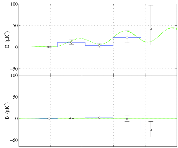
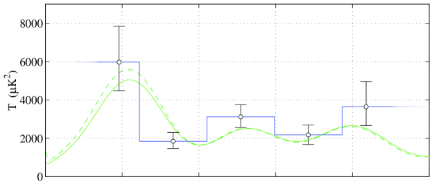
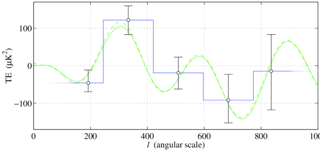
Figure 3: Results from several likelihood analyses. The top two panels show the ten-parameter $E5$/$B5$ polarization analysis, the third panel shows the $T5$ temperature analysis and the bottom panel shows the five $\it TE$ bands from the $\it T/E/TE5$ joint analysis. All results are presented in flat bandpower units of $l(l+1)C_{l}/{2\pi}$. The blue lines show the piecewise-continuous, flat-bandpower model for the maximum likelihood parameter values, with error bars indicating the 68% central region of the likelihood of each parameter, marginalizing over the other parameter values, analogous to the grey lines in the left panels of Figure 2. In each case, the solid green line is the concordance model used in Paper V and this paper, and the dashed dark-green line is a best-fit model for the WMAPext data from Spergel et al. (2003).

3.3.3 $E$/$\beta_{E}$

This analysis parameterizes the $E$-mode polarization signal as above, as well as the frequency spectral index $\beta_{E}$ of this signal relative to the CMB (such that $\beta=0$ corresponds to a 2.73 K Planck spectrum). As expected, the results for the $E$-mode amplitude are very similar to those for the $E/B$ analysis described above. The result for the spectral index is $\beta_{E}=1.39$ ($-0.21$ to 2.92). The index is consistent with CMB, as $\Lambda(\beta_{E}=0)=0.372$ for a PTE = 0.39. It is inconsistent with synchrotron emission, which is rejected at $2.65\sigma$ ($\Lambda(\beta=-2.9)=3.52$ for a PTE = 0.008). Although the constraint is not strong, it is nevertheless interesting in the context of assessing the level of possible contamination by non-thermal emission, as discussed in §4.

3.3.4 $E/sync$

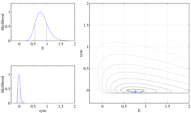
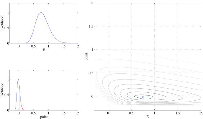
Figure 4: Results of $E/sync$ and $E/point$ two-component polarization analyses. These two analyses, performed to constrain the level of foreground emission in the data set, both use for their first component the same CMB $E$ power spectrum as in the $E/B$ concordance-shape polarization analysis (Figure 2). For the $E/sync$ analysis shown in the upper three panels, the second component is a model for polarized synchrotron emission with $E=B$, flat power spectra and temperature spectral index $\beta=-2.9$ (see §3.3.4). For the $E/point$ analysis shown in the lower panels, the second component models polarized point sources, assuming $E=B$ spectra rising as $l(l+1)C_{l}\propto l^{2}$ and $\beta=-2$ (see §3.3.5). The CMB $E$ component is given in units of amplitude relative to the concordance model, as before. For comparison, the amplitudes of the second components are plotted in units relative to $E=B=8.5\mu K^{2}$ at $l=300$, which is the amplitude of the concordance model $E$ spectrum at that angular scale. (The $E/sync$ plot shows zero likelihood in the region where unphysical negative amplitudes for the second component cause the covariance to be non positive-definite). It is evident that the level of foreground contamination in either of these models is constrained to be well below the level of the observed $E$ signal.

Here and in the next section, we describe two new analyses using two-component models to constrain the level of foreground emission in the data set. In both of these analyses, the first component is the same CMB $E$ power spectrum as in the $E/B$ concordance-shape polarization analysis, with frequency spectral index $\beta=0$. For the $E/sync$ analysis, the second component is defined to be a model of polarized synchrotron emission with $E=B$, flat power spectra (i.e., $l(l+1)C_{l}\propto\rm{constant}$) and a temperature spectral index $\beta=-2.9$. The results of this analysis, given in Table 1 and shown in Figure 4, show that the amplitude of the CMB $E$ component remains consistent with the concordance model, while the amplitude of the synchrotron component is consistent with zero. The $95\%$ upper limit on the synchrotron component, $E=B=0.91\mu K^{2}$, is well below the level of the observed $E$ signal, implying, as discussed in §4, that there is no significant contamination from foreground synchrotron emission in the data set.

3.3.5 $E/point$

A two-component model was also used to test the extent to which the signal in our data could be due to point sources. For this $E/point$ analysis, the second component is a model for polarized point sources, with $E=B$ and $l(l+1)C_{l}\propto l^{2}$ power spectra, for which we have conservatively assumed $\beta=-2$. The results are given in Table 1 and shown in Figure 4. The amplitude of the CMB $E$ component is again consistent with the concordance model, while the point source model component is consistent with zero. The $95\%$ upper limit on the point source component, $E=B=0.98\mu K^{2}$ at $l=300$, is well below the observed signal level. We conclude that the presence of point sources consistent with the data has at most a small effect on the polarization results (see also §4).

3.3.6 Scalar/Tensor

To constrain T/S directly from the polarization data, we perform a two-component likelihood analysis, using for one component the concordance $E$ shape with $B=0$ for the scalars, and for the other component the predicted shapes of $E_{T}$ and $B_{T}$ for the tensors. In principle, because the scalar $B$-mode spectrum is zero, this approach avoids the fundamental sample variance limitations arising from using the temperature spectrum alone. However, the results of the $E5$/$B5$ analysis above indicate that we can place only upper limits on the $E$ and $B-$mode polarization at the angular scales most relevant ($l\lesssim 200$) for the tensor spectra. It is therefore not surprising that our limits on T/S derived from the polarization spectra, as reported in Table 1, remain quite weak.

Table 1: Results of Likelihood Analyses from Polarization Data

					68% interval
analysis	parameter	$l_{\rm{low}}-l_{\rm{high}}$	ML est.	$\left(F^{-1}\right)_{ii}^{1/2}$ error	lower	upper	U.L.(95%)	units
E/B	E	$-$	0.73	$\pm 0.21$	0.53	0.95	$-$	fraction of concordance E
	B	$-$	0.03	$\pm 0.10$	-0.05	0.12	0.25	fraction of concordance E
E5/B5	E1	$28-245$	0.06	$\pm 0.8$	-0.58	1.28	3.6	$~{}\mu{\rm K}^{2}$
	E2	$246-420$	10.5	$\pm 4.1$	6.3	16.6	$-$	$~{}\mu{\rm K}^{2}$
	E3	$421-596$	3.6	$\pm 4.7$	-2.1	8.8	15.2	$~{}\mu{\rm K}^{2}$
	E4	$597-772$	22.1	$\pm 13.0$	9.8	38.8	$-$	$~{}\mu{\rm K}^{2}$
	E5	$773-1050$	42.2	$\pm 40.0$	4.5	96.9	183.4	$~{}\mu{\rm K}^{2}$
	B1	$28-245$	-0.37	$\pm 0.55$	-0.81	0.55	2.12	$~{}\mu{\rm K}^{2}$
	B2	$246-420$	1.0	$\pm 1.7$	-0.57	3.1	6.45	$~{}\mu{\rm K}^{2}$
	B3	$421-596$	1.7	$\pm 3.8$	-1.6	5.6	11.4	$~{}\mu{\rm K}^{2}$
	B4	$597-772$	-1.6	$\pm 6.5$	-6.8	5.7	16.4	$~{}\mu{\rm K}^{2}$
	B5	$773-1050$	-26.7	$\pm 17.9$	-42.9	-7.0	49.3	$~{}\mu{\rm K}^{2}$
E/$\beta_{E}$	E	$-$	0.73	$\pm 0.21$	0.52	0.93	$-$	fraction of concordance E
	$\beta_{E}$	$-$	1.39	$\pm 1.56$	-0.21	2.92	$-$	temperature spectral index
E/sync	E	$-$	0.76	$\pm 0.21$	0.56	0.99	$-$	fraction of concordance E
	sync	$-$	-0.24	$\pm 0.28$	-0.49	0.21	0.91	$~{}\mu{\rm K}^{2}$
E/point	E	$-$	0.76	$\pm 0.23$	0.55	0.99	$-$	fraction of concordance E
	point	$-$	-0.14	$\pm 0.50$	-0.51	0.30	0.98	$~{}\mu{\rm K}^{2}$ at $l=300$
Scalar/Tensor	S	$-$	0.75	$\pm 0.22$	0.55	1.00	$-$	fraction of concordance S
	T	$-$	-5.70	$\pm 7.5$	-12.0	4.5	24.9	T/(S=1)

parameter correlation matrices
$\phantom{string}{\rm E1}$	$\phantom{string}{\rm E2}$	$\phantom{string}{\rm E3}$	$\phantom{string}{\rm E4}$	$\phantom{string}{\rm E5}$	$\phantom{string}{\rm B1}$	$\phantom{string}{\rm B2}$	$\phantom{string}{\rm B3}$	$\phantom{string}{\rm B4}$	$\phantom{string}{\rm B5}$
$\phantom{string}1$	$-0.137$	$\phantom{string}0.015$	$-0.002$	$\phantom{string}0.000$	$-0.241$	$\phantom{string}0.044$	$-0.004$	$\phantom{string}0.001$	$\phantom{string}0.000$
	$\phantom{string}1$	$-0.110$	$\phantom{string}0.011$	$-0.001$	$\phantom{string}0.026$	$-0.076$	$\phantom{string}0.005$	$-0.001$	$\phantom{string}0.000$
		$\phantom{string}1$	$-0.104$	$\phantom{string}0.011$	$-0.003$	$\phantom{string}0.008$	$-0.026$	$\phantom{string}0.003$	$\phantom{string}0.000$
			$\phantom{string}1$	$-0.108$	$\phantom{string}0.000$	$-0.001$	$\phantom{string}0.002$	$-0.017$	$\phantom{string}0.002$
				$\phantom{string}1$	$\phantom{string}0.000$	$\phantom{string}0.000$	$\phantom{string}0.000$	$\phantom{string}0.002$	$-0.016$
					$\phantom{string}1$	$-0.228$	$\phantom{string}0.024$	$-0.003$	$\phantom{string}0.000$
						$\phantom{string}1$	$-0.103$	$\phantom{string}0.014$	$-0.002$
							$\phantom{string}1$	$-0.132$	$\phantom{string}0.019$
								$\phantom{string}1$	$-0.142$
									$\phantom{string}1$
$\phantom{string}{\rm E}$	$\phantom{string}{\rm B}$	$\phantom{string}{\rm E}$	$\phantom{string}\beta_{E}$	$\phantom{string}{\rm E}$	$\phantom{string}{\rm sync}$	$\phantom{string}{\rm E}$	$\phantom{string}{\rm point}$	$\phantom{string}{\rm S}$	$\phantom{string}{\rm T}$
$\phantom{string}1$	$-0.048$	$\phantom{string}1$	$-0.26$	$\phantom{string}1$	$-0.26$	$\phantom{string}1$	$-0.43$	$\phantom{string}1$	$-0.27$
	$\phantom{string}1$		$\phantom{string}1$		$\phantom{string}1$		$\phantom{string}1$		$\phantom{string}1$

3.4 Temperature Data Analyses and Results for the $T$ Spectrum

3.4.1 $T$/$\beta_{T}$

In this analysis, we use the bandpower shape of the concordance $T$ spectrum, with the amplitude parameter expressed in units relative to that spectrum. The spectral index is relative to the CMB, so that $\beta=0$ corresponds to a 2.73 K Planck spectrum. The amplitude of $T$ has a maximum likelihood value of 1.23 (1.13 to 1.35), and the spectral index $\beta_{T}=0.11$ ($-0.02$ to 0.24). While the uncertainty in the temperature amplitude is dominated by sample variance, the uncertainty in the spectral index is limited only by the sensitivity and fractional bandwidth of DASI. Note that these results and those for $T5$ below have not been corrected for contributions from residual point sources (see Paper II).

3.4.2 $T5$

In the third panel of Figure 3, we present the results of an analysis using five, piecewise-continuous, flat bandpowers to characterize the temperature spectrum. Although these results are entirely dominated by the sample variance in the differenced field, they are consistent with the far more sensitive temperature power spectrum described in Paper II. We include them here and in Paper V, primarily to emphasize that DASI makes measurements simultaneously in all four Stokes parameters.

Table 2: Results of Likelihood Analyses from Temperature Data

					68% interval
analysis	parameter	$l_{\rm{low}}-l_{\rm{high}}$	ML est.	$\left(F^{-1}\right)_{ii}^{1/2}$ error	lower	upper	units
T/$\beta_{T}$	T	$-$	1.23	$\pm 0.10$	1.13	1.35	fraction of concordance T
	$\beta_{T}$	$-$	0.11	$\pm 0.10$	-0.02	0.24	temperature spectral index
T5	T1	$28-245$	5970	$\pm 1460$	4480	7840	$~{}\mu{\rm K}^{2}$
	T2	$246-420$	1840	$\pm 410$	1460	2300	$~{}\mu{\rm K}^{2}$
	T3	$421-596$	3120	$\pm 530$	2560	3750	$~{}\mu{\rm K}^{2}$
	T4	$597-772$	2180	$\pm 460$	1670	2690	$~{}\mu{\rm K}^{2}$
	T5	$773-1050$	3650	$\pm 1080$	2660	4960	$~{}\mu{\rm K}^{2}$

parameter correlation matrices
$\phantom{string}{\rm T1}$	$\phantom{string}{\rm T2}$	$\phantom{string}{\rm T3}$	$\phantom{string}{\rm T4}$	$\phantom{string}{\rm T5}$		stringT	$\phantom{string}\beta_{T}$
$\phantom{string}1$	$-0.104$	$\phantom{string}0.004$	$-0.004$	$-0.002$		$\phantom{string}1$	$0.020$
	$\phantom{string}1$	$-0.090$	$-0.012$	$-0.011$			$1$
		$\phantom{string}1$	$-0.109$	$-0.011$
			$\phantom{string}1$	$-0.142$
				$\phantom{string}1$

3.5 Joint Analyses and Cross Spectra Results: $\it TE$, $\it TB$ and $\it EB$

3.5.1 $\it T/E/TE$

In Figure 5, we present results of a three-parameter single-bandpower analysis of the $T$ and $E$ spectra, and the $\it TE$ cross correlation spectrum, using bandpower shapes from the concordance model. The $T$ and $E$ constraints are quite similar to those from the $E$/$B$, $E$/$\beta_{E}$ and $T$/$\beta_{T}$ analyses described above, as expected. The additional result here is the $\it TE$ correlation, which has a maximum likelihood value of 1.08 (0.73 to 1.43). The data are in excellent agreement with concordance model expectations.

For the no $\it TE$-correlation hypothesis, we find a likelihood ratio $\Lambda({\it TE}=0)=4.20$ with a PTE of 0.0038; the no correlation hypothesis is rejected at 2.90$\sigma$, a considerable improvement over the $\it TE$ results presented in Paper V. Note that under the ${\it TE}=0$ hypothesis, negative and positive $\it TE$ are equally likely, so the probability of falsely detecting a positive $\it TE$ correlation at this level is PTE = 0.0019, or 3.11$\sigma$.

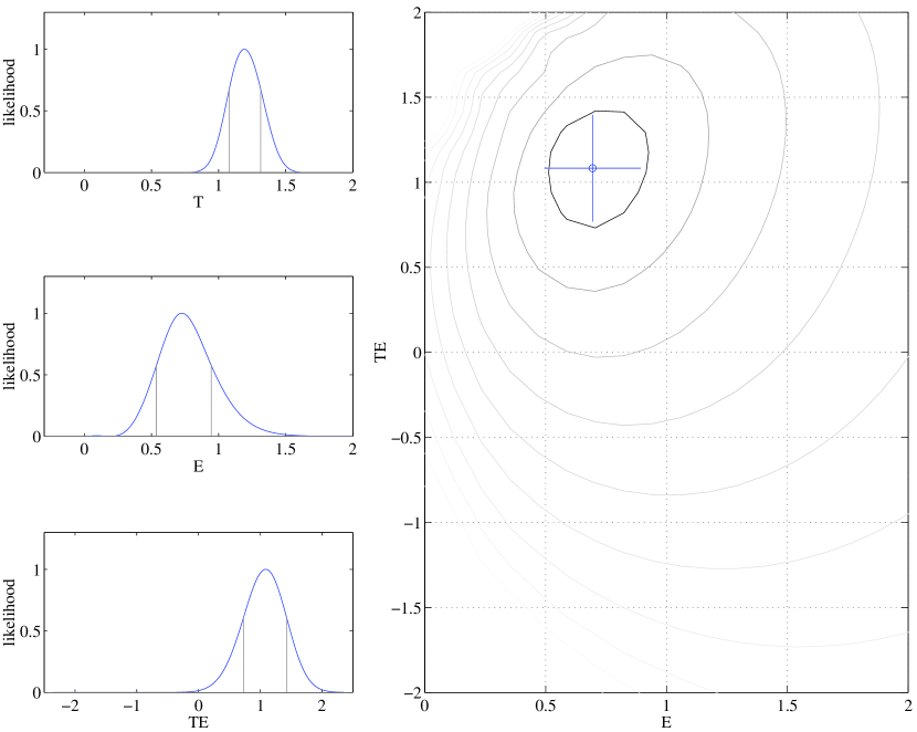
Figure 5: Results from the 3-parameter shaped bandpower $T$/$E$/$\it TE$ joint analysis. Spectral shapes are as predicted for the concordance model, and the units are relative to that model. The layout of the plot is analogous to Figure 2. The two dimensional distribution in the right panel is marginalized over the $T$ dimension.

3.5.2 $\it T/E/TE5$

This is a seven-parameter analysis using single shaped band powers for $T$ and $E$, and five piecewise-continuous, flat bandpowers for the $\it TE$ cross correlation. The $B$-mode polarization is explicitly set to zero for this analysis. The $T$ and $E$ constraints are again similar to the values for the other analyses where these parameters appear. The interesting result here is the $\it TE$ spectrum, shown in the bottom panel of Figure 3. The bandpower results show considerable improvement from the results presented in Paper V, and trace the specific predictions of the concordance model.

3.5.3 $\it T/E/B/TE/TB/EB$

Our last analysis is a six shaped-bandpower analysis for the three individual spectra $T$, $E$ and $B$, together with the three possible cross-correlation spectra $\it TE$, $\it TB$ and $\it EB$. Although there is no evidence for any $B$-mode signal, we include the $B$ cross-spectra for completeness. Since the $\it TB$ and $\it EB$ spectra are expected from theory to be zero, we preserve the symmetry of the analysis between $E$ and $B$ by parameterizing them in terms of the $\it TE$ and $E$ shapes, respectively. The results for $T$, $E$, $B$ and $\it TE$ are again similar to those obtained in the other analyses. As expected under the concordance model, there is no detection of $\it EB$ or $\it TB$.

Table 3: Results of Likelihood Analyses From Joint Temperature-Polarization Data

					68% interval
analysis	parameter	$l_{\rm{low}}-l_{\rm{high}}$	ML est.	$\left(F^{-1}\right)_{ii}^{1/2}$ error	lower	upper	units
T/E/TE	T	$-$	1.17	$\pm 0.10$	1.08	1.31	fraction of concordance T
	E	$-$	0.69	$\pm 0.20$	0.54	0.94	fraction of concordance E
	TE	$-$	1.08	$\pm 0.31$	0.74	1.41	fraction of concordance TE
T/E/TE5	T	$-$	1.17	$\pm 0.10$	1.10	1.32	fraction of concordance T
	E	$-$	0.78	$\pm 0.21$	0.64	1.09	fraction of concordance E
	TE1	$28-245$	-45.9	$\pm 24.3$	-69.3	-11.2	$~{}\mu{\rm K}^{2}$
	TE2	$246-420$	121.9	$\pm 30.7$	82.9	159.8	$~{}\mu{\rm K}^{2}$
	TE3	$421-596$	-19.0	$\pm 41.0$	-62.2	23.0	$~{}\mu{\rm K}^{2}$
	TE4	$597-772$	-91.8	$\pm 60.5$	-152.5	-22.9	$~{}\mu{\rm K}^{2}$
	TE5	$773-1050$	-14.4	$\pm 129.3$	-117.8	83.4	$~{}\mu{\rm K}^{2}$
T/E/B/TE/TB/EB	T	$-$	1.17	$\pm 0.10$	1.08	1.30	fraction of concordance T
	E	$-$	0.68	$\pm 0.20$	0.56	0.98	fraction of concordance E
	B	$-$	0.02	$\pm 0.09$	-0.03	0.15	fraction of concordance E
	TE	$-$	1.17	$\pm 0.30$	0.84	1.52	fraction of concordance TE
	TB	$-$	0.14	$\pm 0.24$	-0.16	0.35	fraction of concordance TE
	EB	$-$	-0.19	$\pm 0.10$	-0.31	-0.10	fraction of concordance E

parameter correlation matrices

$\phantom{string}{\rm T}$

$\phantom{string}{\rm E}$

$\phantom{string}{\rm TE1}$

$\phantom{string}{\rm TE2}$

$\phantom{string}{\rm TE3}$

$\phantom{string}{\rm TE4}$

$\phantom{string}{\rm TE5}$

$\phantom{string}{\rm T}$

$\phantom{string}{\rm E}$

$\phantom{string}{\rm B}$

$\phantom{string}{\rm TE}$

$\phantom{string}{\rm TB}$

$\phantom{string}{\rm EB}$

$\phantom{string}1$

$\phantom{string}0.068$

$-0.159$

$\phantom{string}0.303$

$-0.037$

$-0.126$

$-0.010$

$\phantom{string}1$

$\phantom{string}0.046$

$-0.014$

$\phantom{string}0.299$

$\phantom{string}0.044$

$\phantom{string}0.018$

$\phantom{string}1$

$-0.146$

$\phantom{string}0.484$

$-0.045$

$-0.150$

$\phantom{string}0.001$

$\phantom{string}1$

$\phantom{string}0.009$

$\phantom{string}0.407$

$-0.079$

$-0.310$

$\phantom{string}1$

$-0.127$

$\phantom{string}0.013$

$\phantom{string}0.039$

$\phantom{string}0.001$

$\phantom{string}1$

$-0.018$

$\phantom{string}0.082$

$-0.345$

$\phantom{string}1$

$-0.083$

$-0.099$

$-0.002$

$\phantom{string}1$

$-0.216$

$-0.014$

$\phantom{string}1$

$-0.045$

$\phantom{string}0.004$

$\phantom{string}1$

$\phantom{string}0.295$

$\phantom{string}1$

$-0.058$

$\phantom{string}1$

$\phantom{string}1$

$\phantom{string}{\rm T}$

$\phantom{string}{\rm E}$

$\phantom{string}{\rm TE}$

$\phantom{string}1$

$\phantom{string}0.036$

$\phantom{string}0.276$

$\phantom{string}1$

$\phantom{string}0.372$

$\phantom{string}1$

4 Discussion

The analysis of the 3-year DASI data set supports all of the results presented in Paper V, in particular the detection of $E$-mode CMB polarization consistent with predictions of the standard cosmological model, and inconsistent with any significant contamination from foreground emission. The increased sensitivity of the combined data set permits a more precise characterization of the detected polarization signal, and increasingly sensitive tests for the presence of foreground contamination.

As discussed in §3.1, simple consistency tests with no assumptions about the underlying model show a high confidence detection of polarized signal. When the polarized anisotropy is modeled by a shaped spectrum over the $l$-range spanned by DASI, the data strongly prefer the concordance model shape for the $E$-mode spectrum (see §3.3.1). Assuming the concordance model shape, we detect $E$-mode polarization (at $6.3\sigma$ confidence), as well as the $\it TE$ cross-correlation ($2.9\sigma$), both with significantly increased statistical power over the results in Paper V, and at levels consistent with theoretical expectations. As expected for CMB anisotropies, the level of the $B$-mode polarization is consistent with zero, with an upper limit significantly below the $E$-mode detection.

The five piecewise-continuous bandpower analysis presented in §3.3.2 further demonstrates that the detailed shape of the $E$-mode anisotropy is consistent with the concordance predictions. The $E$-mode bandpowers place a stringent upper limit in the lowest $l$-range band, with maximum likelihood values in the remaining four bands that are consistent with the damped concordance model, but inconsistent with a simple $l(l+1)C_{l}\propto l^{2}$ power law. As shown in Figure 3 (§3.5.2), the $\it TE$ angular power spectrum provides a highly specific test of the spectral shape, as the predicted $\it TE$ correlation crosses zero five times over the angular range covered by the DASI measurements.

Of the known foregrounds at 30 GHz, diffuse Galactic synchrotron emission and radio point sources are of the greatest concern. (As discussed in Paper V, neither free-free nor dust emission, of either the thermal or spinning variety, is expected to contribute any significant polarized signal to the DASI data.) It was for this reason that the two DASI fields were carefully selected from regions of exceptionally low emission in the Haslam maps (Haslam et al., 1981), confirmed at higher frequency by the WMAP synchrotron maps to be clean regions of sky (Bennett et al., 2003) (see Figure 1). The two fields were also selected from those with no detectable point sources from the original 32 DASI temperature anisotropy fields.

While no published maps exist of the polarized synchrotron emission toward our fields, the DASI data themselves set stringent constraints on the allowed level of diffuse synchrotron. As discussed in §3.3.4, a two-component model, designed specifically to probe for synchrotron emission, finds that the amplitude of a synchrotron component with $\beta=-2.9$ is consistent with zero, with an upper limit well below the level of the CMB $E$-mode signal. The $E$-mode spectral index constraint, improved from Paper V, indicates that the polarized signal is consistent with CMB; a signal with the expected synchrotron spectral index $\beta=-2.9$ is rejected at the 2.7$\sigma$ level. The detection of the $\it TE$ correlation is strong evidence that the polarized signal shares a common origin with the total intensity signal, a signal which has been robustly demonstrated in Paper II, Paper V and here to be consistent with CMB in both its frequency spectral index ($\beta=0.11$ ($-0.02$ to $0.24$) from §3.4.1 above) and angular power spectrum. Moreover, the pronounced asymmetry of the $E$-mode and $B$-mode levels allowed by DASI is in sharp contrast to the symmetric predictions for sources of foreground emission (Zaldarriaga, 2001).

Since no catalog of faint polarized sources exists over our observing region, and it is not possible to identify from total intensity which point sources will have the strongest polarized flux, it is impracticable to project sources out of the polarization analyses. Nevertheless we can estimate the level of residual contamination in the data. A new, two-component analysis performed on the 3-year data set finds that the amplitude of a point-source component, with a conservative spectral index $\beta=-2$, is consistent with zero, with an upper limit well below the level of the CMB $E$-mode signal (see §3.3.5).

We analyzed maps of the differenced fields directly for evidence of individual sources appearing above the noise floor. The pixel value distributions are consistent with instrument noise plus a Gaussian signal, and show no sign of excess tails due to discrete sources. The sensitivity of our maps is such that point sources with beam-attenuated polarized flux greater than 15 mJy would have been clearly detected.

In Paper V, we also presented a Monte Carlo analysis of the expected point-source contribution, based on available knowledge of the source populations. The number-flux counts used in the simulation (determined from the 2000 DASI temperature data (see Paper V)) are consistent with the WMAP results on $dN/dS$ (Bennett et al., 2003), and while there is a dearth of data concerning the distribution of source polarization fractions at 30 GHz, a recent 18.5 GHz study (Ricci et al., 2004) reports a distribution similar to the one assumed in our calculations. These simulations suggest a mean bias of the $E$ parameter of 0.04 with a standard deviation of 0.05. We therefore conclude that there is neither the expectation of, nor evidence in the data for, any significant contamination by polarized point sources.

5 Conclusion

DASI has detected $E$-mode CMB polarization with high confidence ($6.3\sigma$ with the addition of the new data), and has detected the $\it TE$ correlation at the $2.9\sigma$ level. The shape and amplitude of the detected $E$-mode angular power spectrum are in agreement with theoretical predictions based on the CMB temperature measurements. These results lend strong support to the underlying theoretical framework for the generation of CMB anisotropy and point toward a promising future for the field — a future which includes the detailed characterization of the $E$-mode spectrum, the detection on small scales of $B$-modes from gravitational lensing, and the tantalizing prospect of constraining inflationary models via the detection of large-scale $B$-modes from primordial gravitational waves.

The DASI polarization results demonstrate the beauty of using interferometric techniques to provide well-matched filters for $E$- and $B$-mode measurements, and the inherent power of interferometers to reject uncorrelated noise and control systematics. The DASI results would continue to improve with increased integration time, however the sensitivity required for the detection of the $B$-mode signatures demands large arrays, beyond the current scaling limitations of existing correlators. While there are currently no plans to upgrade DASI as an interferometer, advances in technology may once again make interferometry an attractive choice for pursuing the extraordinary control of systematics required by the next generation of CMB polarization experiments.

We thank Ben Reddall, Eric Sandberg and Allan Day for their dedicated and professional support to the DASI polarization experiment while they wintered at the NSF Amundsen-Scott South Pole research station. We are indebted to Bill Holzapfel and Mark Dragovan, whose early contributions to the DASI experiment were essential to the success of the program, and to the CBI team led by Tony Readhead, in particular to John Cartwright, Steve Padin and Martin Shepherd. We are grateful for expert technical assistance from Jacob Kooi, Charlie Kaminski, Ellen LaRue, Bob Pernic, Bob Spotz and Mike Whitehead. We thank the U.S. Antarctic Program and the Raytheon Polar Services Corporation for their support of the project. The DASI project is supported by NSF grant OPP-0094541. This research was also supported in part by NSF grant PHY-0114422 to the Kavli Institute for Cosmological Physics, a NSF Physics Frontier Center. NWH acknowledges support from a Charles H. Townes Fellowship at the U.C.B. Space Sciences Laboratory. JMK acknowledges support from a Millikan Fellowship at Caltech.

References

- Bennett et al. (2003) Bennett, C. L., Hill, R. S., Hinshaw, G., Nolta, M. R., Odegard, N., Page, L., Spergel, D. N., Weiland, J. L., Wright, E. L., Halpern, M., Jarosik, N., Kogut, A., Limon, M., Meyer, S. S., Tucker, G. S., & Wollack, E. 2003, ApJS, 148, 97, astro-ph/0302208
- Bond et al. (1998) Bond, J. R., Jaffe, A. H., & Knox, L. 1998, Phys. Rev. D, 57, 2117
- Christensen et al. (2001) Christensen, N., Meyer, R., Knox, L., & Luey, B. 2001, Classical and Quantum Gravity, 18, 2677
- Halverson et al. (2002) Halverson, N. W., Leitch, E. M., Pryke, C., Kovac, J., Carlstrom, J. E., Holzapfel, W. L., Dragovan, M., Cartwright, J. K., Mason, B. S., Padin, S., Pearson, T. J., Readhead, A. C. S., & Shepherd, M. C. 2002, ApJ, 568, 38, astro-ph/0104489
- Haslam et al. (1981) Haslam, C. G. T., Klein, U., Salter, C. J., Stoffel, H., Wilson, W. E., Cleary, M. N., Cooke, D. J., & Thomasson, P. 1981, A&A, 100, 209
- Hu & Dodelson (2002) Hu, W. & Dodelson, S. 2002, ARA&A, 40, 171
- Kogut et al. (2003) Kogut, A., Spergel, D. N., Barnes, C., Bennett, C. L., Halpern, M., Hinshaw, G., Jarosik, N., Limon, M., Meyer, S. S., Page, L., Tucker, G. S., Wollack, E., & Wright, E. L. 2003, ApJS, 148, 161, astro-ph/0302213
- Kovac (2003) Kovac, J. M. 2003, PhD thesis, University of Chicago
- Kovac et al. (2002) Kovac, J. M., Leitch, E. M., Pryke, C., Carlstrom, J. E., Halverson, N. W., & Holzapfel, W. L. 2002, Nature, 420, 772, astro-ph/0209478
- Leitch et al. (2002a) Leitch, E. M., Kovac, J. M., Pryke, C., Carlstrom, J. E., Halverson, N. W., Holzapfel, W. L., Reddall, B., & Sandberg, E. S. 2002a, Nature, 420, 763, astro-ph/0209476
- Leitch et al. (2002b) Leitch, E. M., Pryke, C., Halverson, N. W., Carlstrom, J. E., Kovac, J., Holzapfel, W. L., Dragovan, M., Cartwright, J. K., Mason, B. M., Padin, S., Pearson, T. J., Readhead, A. C. S., & Shepherd, M. C. 2002b, ApJ, 568, 28, astro-ph/0104488
- Pryke et al. (2002) Pryke, C., Halverson, N. W., Leitch, E. M., Kovac, J., Carlstrom, J. E., Holzapfel, W. L., & Dragovan, M. 2002, ApJ, 568, 46, astro-ph/0104490
- Ricci et al. (2004) Ricci, R., Prandoni, I., Gruppioni, C., Sault, R. J., & De Zotti, G. 2004, A&A, 415, 549
- Spergel et al. (2003) Spergel, D. N., Verde, L., Peiris, H. V., Komatsu, E., Nolta, M. R., Bennett, C. L., Halpern, M., Hinshaw, G., Jarosik, N., Kogut, A., Limon, M., Meyer, S. S., Page, L., Tucker, G. S., Weiland, J. L., Wollack, E., & Wright, E. L. 2003, ApJS, 148, 175, astro-ph/0302209
- Zaldarriaga (2001) Zaldarriaga, M. 2001, Phys. Rev. D, 64, 103001+