Faraday screens associated with
local molecular clouds

Polarization observations at $\lambda\,21\,\mbox{cm}$ and $\lambda\,18\,\mbox{cm}$ towards the local Taurus molecular cloud complex were made with the Effelsberg 100-m telescope. Highly structured, frequency-dependent polarized emission features were detected. We discuss polarization minima with excessive rotation measures located at the boundaries of molecular clouds. These minima get less pronounced at the higher frequencies. The multi–frequency polarization data have been successfully modeled by considering magneto–ionic Faraday screens at the surface of the molecular clouds. Faraday rotated background emission adds to foreground emission towards these screens in a different way than in its surroundings. The physical size of the Faraday screens is of the order of $2$ pc for $140$ pc distance to the Taurus clouds. Intrinsic rotation measures between about $-18$ rad m^-2 to $-30$ rad m^-2 are required to model the observations. Depolarization of the background emission is quite small (compatible with zero), indicating a regular magnetic field structure with little turbulence within the Faraday screens. With observational constraints for the thermal electron density from H$\alpha$ observations of less than $0.8$ cm^-3 we conclude that the regular magnetic field strength along the line of sight exceeds $20\leavevmode\nobreak\ \mu$G, to account for the observed rotation measure. We discuss some possibilities for the origin of such strong and well ordered magnetic fields. The modeling also predicts a large-scale, regularly polarized emission in the foreground of the Taurus clouds which is of the order of $0.18$ K at $\lambda\,21\,\mbox{cm}$. This in turn constrains the observed synchrotron emission in total intensity within $140$ pc of the Taurus clouds. A lower limit of about $0.24$ K, or about $1.7$ K/kpc, is required for a perfectly ordered magnetic field with intrinsic ($\sim 75\%$) percentage polarization. Since this is rather unlikely to be the case, the fraction of foreground synchrotron emission is even larger. This amount of synchrotron emission is clearly excessive when compared to previous estimates of the local synchrotron emissivity.

1 Introduction

For large areas of the sky the polarization properties of Galactic radio emission are not well known in detail. Most information came from early large–scale surveys of the northern sky carried out at Jodrell Bank and Cambridge with $1.4$ GHz being the highest frequency used (Bingham bing (1966)). The angular resolution of all these surveys was low. Later the Dwingeloo–surveys were carried out in the frequency range from $408$ MHz up to $1415$ MHz (Brouw & Spoelstra brouw (1976)). They have angular resolutions of $0\aas@@fstack{\circ}6$ at 1411 MHz or less at the lower frequencies and are absolutely calibrated, but severely under-sampled. Details of the polarization structures require fully sampled measurements at arc-minute angular resolution. A number of observations were made during the last decade using synthesis arrays as well as single-dish telescopes. Polarization observations by Junkes et al. (junk (1987)), Wieringa et al. (wie (1993)), Duncan et al. (dunc97 (1997), dunc99 (1999)), Gray et al. (gray1 (1998), gray2 (1999)), Uyanıker et al. (buII (1999)), Haverkorn et al. (haver (2000)), Gaensler et al. (gaens (2001)) revealed highly varying polarized structures, which are not correlated to structure variations seen in total intensity maps. These findings called for a systematic approach and new polarization surveys were initiated.

Here we report on follow-up observations at $\lambda\,18\,\mbox{cm}$ of the Effelsberg $\lambda\,21\,\mbox{cm}$ ”Medium Galactic Latitude Survey” (EMLS, Reich et al., in preparation). This survey covers the northern Galactic plane in the range of $\pm 20^{\circ}$. The first EMLS maps (Uyanıker et al. buII (1999)) show an unexpected richness in structure of the polarized emission, which indicates significant variations in the properties of the magneto-ionic medium. Since the polarization structures are not associated with total intensity enhancements or depressions, the interpretation of Faraday modulation of an intrinsically polarized background seems the most likely explanation for the observations.

The physical parameters of the Faraday rotating regions, the Faraday screens, are of particular interest as they reflect local conditions of the magneto-ionic interstellar medium, which deviate from the average parameters derived from the analysis of rotation measure ($RM$) from pulsars or extragalactic sources. The average density of thermal electrons in the Galactic plane is about $0.03$ cm^-3 and the average of the regular magnetic field along the line of sight is about $1$ to $2\leavevmode\nobreak\ \mu$G (Taylor & Cordes tay (1993); Comez et al. com (2001); Cordes & Lazio cord (2003)). However, local bubbles with $RM$s exceeding $100$ rad m^-2 are known to exist in the Galaxy (e.g. Gray et al. gray1 (1998); Gaensler et al. gaens (2001); Uyanıker et al. buIII (2003)). Such large $RM$ values need kpc-size structures to originate within the average magneto-ionic medium and strongly suggest significant local enhancements of the magnetic field strength and/or the thermal electron density. The total magnetic field strength was estimated to be about $5$ to $6\leavevmode\nobreak\ \mu$G in the solar vicinity (Strong et al. strong (2000)). Even in the unlikely case that the regular component along the line of sight locally has that value, an excessive size of the Faraday screens of some hundred parsec is required.

The key problem is the unknown distance of the Faraday screens and this makes any estimate of their physical parameters rather uncertain. Distance information can be obtained by spectral line observations of either H i, $\@element{\mathrm{CO}}$ or recombination lines of neutral hydrogen clouds, molecular clouds or H ii regions associated with Faraday screens. The Taurus–Auriga region seems to be quite suited for such an investigation. The large molecular and dust cloud complexes are at a distance of about $140$ pc, and it is therefore possible to resolve structures on pc–scales with arc-min angular resolution. In addition the Taurus-Auriga complex is located at medium latitudes well below the Galactic Plane, so that confusion with the intense emission from the Galactic disk is not important. The maps from the EMLS revealed a number of polarized enhancements or depressions apparently related to molecular material. In order to derive physical properties of the associated Faraday screens we have complemented the $\lambda\,21\,\mbox{cm}$ survey data of the Taurus–Auriga region by $\lambda\,18\,\mbox{cm}$ observations to derive the depolarization properties and the rotation measures. We modeled the polarization data in order to constrain the physical parameters of the Faraday screens by taking into account foreground and background emission.

2 Observations and data reduction

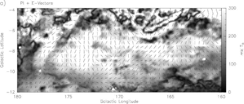
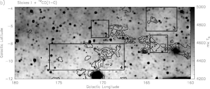
Figure 1: a) Section from the $\lambda\,21\,\mbox{cm}$ ”Medium Galactic Latitude Survey” including absolute calibration showing polarized intensities with polarization vectors overlaid in E–field direction. b) the same for $\lambda\,21\,\mbox{cm}$ total intensities. These include the $2.7$ K cosmic microwave background. Overlaid contours show integrated $\@element{\mathrm{CO}}$ emission from the survey by Dame et al. (dame (2001)). The four fields observed at $\lambda\,18\,\mbox{cm}$ are marked and labeled.

The $\lambda\,21\,\mbox{cm}$ observations for the EMLS were recently completed and are presently in final reduction stage. The data covering the Taurus-Auriga region extending below the Galactic plane from $l=150^{\circ}$ to $l=190^{\circ}$ were extracted and reduced by Wolleben (woll (2001)) following the survey reduction procedures. In brief, total intensities and linear polarization were measured simultaneously with sensitivities of $15$ mK for Stokes $I$ and $8$ mk for Stokes $U$ and $Q$ at an angular resolution of $9\aas@@fstack{\prime}35$. The observing, reduction and calibration methods of the survey and selected maps from different regions along the Galactic plane were already published by Uyanıker et al. (buI (1998), buII (1999)). The absolute calibration of the total intensity data was done in the usual way by adding the missing large-scale structure from the absolutely calibrated Stockert $\lambda\,21\,\mbox{cm}$ survey (Reich & Reich rei86 (1986)). The absolute calibration of the Effelsberg polarization survey data relied so far on Dwingeloo polarization data (Brouw & Spoelstra brouw (1976)). However, the Dwingeloo survey is rather incomplete in coverage and largely under-sampled, so only a few measurements were available for the Taurus–Auriga region. We therefore made use of the new polarization survey carried out with the DRAO 26-m telescope at 1.41 GHz, which consists of fixed declination scans being fully sampled along right-ascension. They are separated in declination by 1^∘ to 2^∘. A brief description of the survey methods and preliminary results was already given by Wolleben et al. (woll1 (2004)). The DRAO data for Stokes $U$ and $Q$ were compared with the corresponding Effelsberg maps both being convolved with a 6^∘-wide Gaussian and the differences were added to the original Effelsberg $U$ and $Q$ maps, respectively.

The $\lambda\,21\,\mbox{cm}$ Taurus–Auriga map in total intensity and polarization was discussed in detail by Wolleben (woll (2001)) with large-scale polarization correction using Dwingeloo data. A section of this map with the new large-scale DRAO polarization data as described above is displayed in Figs. 1a and b showing polarized and total intensities. Total intensities were overlayed with the distribution of integrated $\@element{\mathrm{CO}}$ emission as observed by Dame et al. (dame (2001)) tracing numerous molecular gas clouds in this region.

Follow–up observations of selected fields, where significant polarization structure was seen, were done using the Effelsberg 100-m telescope at two frequencies around $\lambda\,18\,\mbox{cm}$ ($1660$ MHz and $1713$ MHz) in September 2001. The same receiver as for the $\lambda\,21\,\mbox{cm}$ EMLS was used, but a different HF-filter was selected to suppress interference out of the $\lambda\,18\,\mbox{cm}$ band. The observations were done simultaneously for both frequencies by utilizing two identical IF-polarimeters. Both have an effective bandwidth of $14$ MHz. The fields were mapped two times in orthogonal scanning directions along Galactic latitude and Galactic longitude, in a similar way to the $\lambda\,21\,\mbox{cm}$ EMLS observations. The angular resolution was $7\aas@@fstack{\prime}87$ at $1660$ MHz and $7\aas@@fstack{\prime}70$ at $1713$ MHz, respectively. The maps were fully sampled at $3\arcmin$. 3C286 served as the main calibration source with a flux density of $13.3$ Jy at $1660$ MHz and $13.1$ Jy at $1713$ MHz, respectively. The percentage polarization was taken as $9.6$% at a polarization angle of $33$°. In addition, 3C138 and 3C48 were used as secondary calibrators. The higher frequency maps have been convolved with a Gaussian to match the $9\aas@@fstack{\prime}35$ resolution of the $\lambda\,21\,\mbox{cm}$ EMLS. The rms–noise measured were $15$ mK (1408 MHz), $16$ mK ($1660$ MHz) and $19$ mK ($1713$ MHz) for total intensities and $8$ mK, $9$ mK, and $10$ mK for Stokes $U$ and $Q$, respectively. The same conversion factor of $T_{\mathrm{B}}/S=2.12\pm 0.02$ mK/Jy at $\lambda\,21\,\mbox{cm}$ (Uyanıker et al. buI (1998)) applies for all frequencies.

In order to remove temperature gradients due to varying ground and atmospheric radiation from the maps, a linear baseline was subtracted from each subscan. This procedure also affects real sky emission of large spatial extent, this emission is usually recovered by absolutely calibrated data. However, other than at $\lambda\,21\,\mbox{cm}$ there exist no absolutely calibrated data at $\lambda\,18\,\mbox{cm}$ and we calibrated the maps in the following way: The temperature spectral index of the Galactic synchrotron emission $\beta^{\mathrm{I}}$ ($T_{\mathrm{B}}\propto\nu^{\beta^{\mathrm{I}}}$) was adopted to be $\beta^{\mathrm{I}}\approx-2.7$ in the Taurus area following the results of Reich & Reich (rei88 (1988)) for the frequency range between $408$ MHz and $1420$ MHz. We assumed the same spectral index also for the large-scale (LS) polarized intensities ($\beta^{\mathrm{PI}}_{\mathrm{LS}}$) and calculated an average offset for the $\lambda\,18\,\mbox{cm}$ maps from that of the $\lambda\,21\,\mbox{cm}$ map. Rotation measures ($RM$s) across the Taurus region were determined by Spoelstra (spoel72 (1972)) using data between 408 MHz and 1411 MHz. The $RM$s are very low everywhere varying around zero and we assume an average $RM_{\mathrm{LS}}$ of $\rm 0\leavevmode\nobreak\$ rad m^-2 to calculate from the extrapolated large-scale polarized intensity the offsets for the $\lambda\,18\,\mbox{cm}$ $U$ and $Q$ maps, respectively. Since the frequency differences are not very large we believe that the applied extrapolation closely resembles absolutely calibrated $\lambda\,18\,\mbox{cm}$ polarization data and we expect only marginal effects on the small-scale polarized structure analysis we are interested in.

3 Results

3.1 Polarization maps

Table 1: Observed values for the center of the identified Faraday screens in Field 4 (see Fig. 1b). The observed spectral index of the polarized intensity $\beta^{\mathrm{PI}}_{\mathrm{obs}}$ and the observed $RM_{\mathrm{obs}}$ were calculated using $1408$ MHz and $1660$ MHz data. Errors in $PI$ are $11\leavevmode\nobreak\$mK ($1408$ MHz), $13\leavevmode\nobreak\$mK ($1660$ MHz), and $14\leavevmode\nobreak\$mK ($1713$ MHz).

			$1408$ MHz		$1660$ MHz		$1713$ MHz
Object	$l$	$b$	$PI$	$PA$	$PI$	$PA$	$PI$	$PA$	$\beta^{\mathrm{PI}}_{\mathrm{obs}}$	$RM_{\mathrm{obs}}$
	deg	deg	mK	deg	mK	deg	mK	deg		rad m-2
a	170.3	$-9.0$	144	$-29\pm 2$	136	$-25\pm 2$	132	$-23\pm 2$	$-0.4\pm 0.9$	$-5\pm 4$
b	170.45	$-9.4$	207	$-29\pm 1$	168	$-22\pm 2$	163	$-21\pm 2$	$-1.3\pm 0.7$	$-9\pm 3$
c	170.25	$-10.0$	79	$-32\pm 3$	104	$-33\pm 3$	102	$-30\pm 3$	$1.7\pm 1.3$	$1\pm 6$
d	169.75	$-9.7$	97	$-17\pm 2$	124	$-28\pm 2$	118	$-25\pm 2$	$1.5\pm 1.1$	$15\pm 5$
e	169.3	$-9.55$	115	$-5\pm 2$	121	$-24\pm 2$	108	$-23\pm 3$	$0.3\pm 1$	$26\pm 5$
f	171.4	$-8.95$	130	$-18\pm 2$	142	$-12\pm 2$	147	$-11\pm 2$	$0.5\pm 0.9$	$-8\pm 4$
g	168.15	$-8.6$	75	$-20\pm 3$	103	$-30\pm 3$	90	$-29\pm 3$	$2.0\pm 1.4$	$14\pm 6$
h	174.53	$-10.18$	125	$-77\pm 2$	124	$-51\pm 2$	106	$-55\pm 3$	$0\pm 1$	$-36\pm 4$
i	169.35	$-10.65$	109	$-23\pm 2$	117	$-22\pm 2$	111	$-20\pm 2$	$0.4\pm 1.1$	$-1\pm 5$

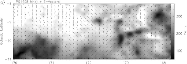
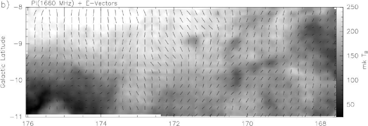
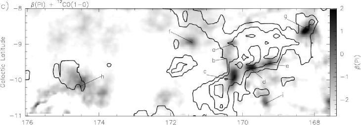
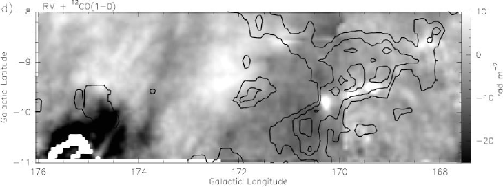
Figure 2: Field 4: Polarized intensity at 1408 MHz a) and $1660$ MHz b) with selected polarization E-vectors superimposed, which are shown for every third pixel (separation $12\arcmin$). The temperature spectral index of the polarized intensity is shown in c), where in addition the individual objects being modeled are indicated. The distribution of $RM$ is shown in d). $RM$s are calculated from the polarization data obtained at 1408 MHz and $1660$ MHz. Figures 2c and d show in addition superimposed contours of integrated $\@element{\mathrm{CO}}$ emission.

The $\lambda\,18\,\mbox{cm}$ maps show – like the $\lambda\,21\,\mbox{cm}$ map – no remarkable structures in total intensities. All maps show smooth diffuse emission varying mainly with Galactic latitude and a large number of unrelated extragalactic sources are superimposed. The polarization structures for Fields 1 to 3 (see Fig. 1b) are rather similar for all wavelengths with marginal differences in structure and polarization angles. Neither of these structures show unusual spectral indices of the polarized emission, they are not spatially associated with molecular clouds or any other known objects and originate in the ISM at an unknown distance. For the majority of polarization structures in these fields, the present frequency range and separation seems not adequate for a reliable analysis of the Faraday effects towards these features.

In Field 4 there are a number of small-scale polarization minima, which spatially coincide with the molecular cloud covered in this field. These minima are obviously aligned to the boundary of the cloud. They show rather clear differences in intensity and thus in spectral index, as well as in the distribution of polarization angles between $\lambda\,18\,\mbox{cm}$ and $\lambda\,21\,\mbox{cm}$. For the nine intensity minima we intend to model, we list their positions, measured polarization data, spectral index and $RM$ in Table 1. Spectral index and $RM$ are calculated from the 1408 MHz and 1660 MHz data. No simple fit based on a $\lambda$ or $\lambda^{2}$ dependence including all data was possible, reflecting the complex situation of polarized emission transfer through a Faraday screen. Figures 2a and b show the observed polarized intensities at 1408 MHz and $1660$ MHz with selected E-vectors superimposed. Figure 2c displays the temperature spectral index for the polarized intensity calculated from:

$$\beta^{\mathrm{PI}}=\frac{\log(PI_{\mathrm{1}}/PI_{\mathrm{2}})}{\log(\nu_{\mathrm{1}}/\nu_{\mathrm{2}})}\ ,$$ (1)

with the frequencies $\nu$ and $\nu_{\mathrm{2}}>\nu_{\mathrm{1}}$. The spectrum of the large-scale emission is close to $\beta^{\mathrm{PI}}_{\mathrm{obs}}=-2.7$, which was the assumption made earlier, while the Faraday screens all show flat or inverted spectra with larger intensities at $\lambda\,18\,\mbox{cm}$ than at $\lambda\,21\,\mbox{cm}$. In Fig. 2d we show the distribution of $RM$ which we have calculated on the basis of the 1408 MHz and $1660$ MHz observations. While $RM_{\mathrm{LS}}=0$ rad m^-2 was assumed for the large-scale emission we find clear $RM$ deviations in the Faraday screen directions.

4 Discussion

4.1 Additional data for the analysis

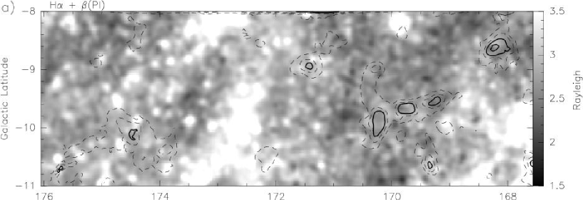
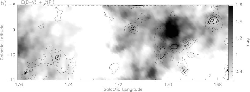
Figure 3: a) The relevant section from the ”full-sky H-alpha map” combined by Finkbeiner (haref (2003)). b) The map of Schlegel et al. (schlegel (1998)) showing interstellar reddening $E_{\mathrm{B-V}}$. Both images show selected contours of the temperature spectral index of the polarized emission superimposed. Dashed lines indicate negative spectral indices and solid lines positive ones.

We searched for additional observations of the Taurus region which might be helpful in the interpretation of the polarization data. $RM$ variations may result from variations of the thermal electron density, which are traced by H$\alpha$ emission. In Fig. 3a we show the H$\alpha$ emission taken from the ”full-sky H-alpha map” which Finkbeiner (haref (2003)) compiled from northern sky (WHAM and VTSS) and southern sky (SHASSA) data. The angular resolution of Finkbeiner’s combined map is $6\arcmin$. No structured H$\alpha$ emission is visible, which might be correlated with the polarized emission features we have measured. The quoted H$\alpha$ sensitivity of $0.52$ Rayleigh is taken as a limit for associated H$\alpha$ emission.

Correlation of polarized emission structures, however, was found with integrated $\@element{\mathrm{CO}}$ emission and also with interstellar absorption. We display a map of the reddening $E_{\mathrm{B-V}}$ in Fig. 3b, which is a reprocessed composite of the DIRBE and IRAS/ISSA maps at $100\leavevmode\nobreak\ \mu$m by Schlegel et al. (schlegel (1998)). The map of Schlegel et al. is believed to trace the dust density more closely than the IRAS $100\leavevmode\nobreak\ \mu$m map. Like the map of integrated $\@element{\mathrm{CO}}$ emission these maps show a remarkable correlation with the polarization maps.

4.2 Faraday screens

The morphology of the observed polarized emission and its variation with frequency suggests that strong Faraday rotation takes place in regions at the surface of molecular clouds. We use a simple model to describe the effect of these Faraday screens on the observed distribution of Galactic polarization. The screen is placed somewhere inside the synchrotron emitting region and modulates the polarized emission passing through it. According to the total intensity observations, where no correlated enhancement is noted, the Faraday screen itself is assumed not to radiate and the noise level of the total intensity maps provides an upper limit for its emission.

Galactic synchrotron emission is generated by cosmic-ray electrons in the Galactic magnetic field. The position angle of synchrotron emission, when corrected for Faraday rotation along the line of sight, is in the direction of the magnetic field component perpendicular to the line of sight. The two emission components in front and behind the Faraday screen are supposed to be independent with different intensities and polarization angles, although they might themselves consist of multiple layers with different magnetic field orientation and/or some internal Faraday dispersion. These emission components are assumed to vary on larger scales than the size of the Faraday screens and therefore to have the same properties across the area modeled. Foreground and background polarization intensities and polarization angles are described in the following by $PI_{\mathrm{fore}}$ and $PA_{\mathrm{fore}}$ or $PI_{\mathrm{back}}$ and $PA_{\mathrm{back}}$, respectively.

The Faraday screen may decrease the polarized intensity of the background emission by depolarization. In addition it changes the background position angle by Faraday rotation. Therefore, the observed emission may increase or decrease relative to its surroundings, depending on the polarization angle orientation of the foreground and the background emission.

The polarization angle $PA$ of linearly polarized radiation is rotated by $\Delta PA$ when passing through the magneto-ionic medium of the Faraday screen and measured at wavelength $\lambda$. The rotation is given by:

$$\Delta PA=RM\cdot\lambda^{2}\ ,$$ (2)

with $RM$, the rotation measure of the Faraday screen:

$$RM=0.81\,B_{\parallel}\,n_{\mathrm{e}}\,l\ .$$ (3)

Here $B_{\parallel}$ is the magnetic field strength component along the line of sight measured in $\mu$G, $n_{\mathrm{e}}$ is the electron density per cm^-3 and $l$ is the size of the Faraday screen along the line of sight measured in pc.

In principle a number of effects are able to lower the observed degree of polarization by depolarization (see Burn burn (1966), Sokoloff et al. soko (1998)). Due to the relatively small spatial extent of the Faraday screens discussed here, along with moderate electron densities and magnetic field strengths, the following mechanisms might potentially contribute:

Beam depolarization:

A variation of the polarization angle across the beam reduces the observed degree of polarization. A rotation measure gradient within the beam can cause such an angle variation. $\Delta RM=17$ rad m^-2$/\mbox{beam}$ at $\lambda\,21\,\mbox{cm}$ would reduce the degree of polarization by $10$%. We do observe such strong gradients towards the Faraday screens in our field, and we conclude that beam depolarization may not be negligible. Therefore, we include depolarization in our model.

Bandwidth depolarization:

An interstellar rotation measure causes the polarization angle to vary over the frequency band of the receiver. A $RM$ of $600$ rad m^-2 at $\lambda\,21\,\mbox{cm}$ is necessary to decrease the degree of polarization by $10$%. Such $RM$s are clearly excessive to those observed here and we conclude that bandwidth depolarization is negligible.

4.3 The model

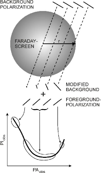
Figure 4: The sketch shows the main components of the model. Polarized emission from behind the Faraday screen (background polarization) is systematically rotated and depolarized as a function of path length through the screen. The superposition of the modified background and the polarized foreground emission leads to a systematic variation of the observed polarized intensity and angle as seen in the $PA$–$PI$ plot.

In the following a Faraday screen is assumed to be a uniform sphere with radius $R$. Elliptical structures were reduced to circulars by normalizing the maximum radius at each position angle of the ellipse to $1$. The path length for radiation passing through the screen will therefore vary systematically with position $r$. With $r$ as the projection of $R$ on the sky, the path length $l$ is given by $l(r)=2\sqrt{R^{2}-r^{2}}$. We also assume a constant electron density $n_{\mathrm{e}}$ and a homogeneous magnetic field ${B}$ inside the sphere with a component $B_{\parallel}$ along the line of sight. Faraday rotation is zero for $r\geq R$. The modified polarization angle $PA_{\mathrm{mod}}$ can be written as

$$PA_{\mathrm{mod}}(r)=PA_{\mathrm{back}}+RM_{\mathrm{int}}(r)\cdot\lambda^{2}$$ (4)

with

$$RM_{\mathrm{int}}(r)=RM_{\mathrm{0}}\cdot l(r)\ .$$ (5)

$RM_{\mathrm{0}}$ is the maximum intrinsic rotation measure of the Faraday screen at $r=0$.

We assume any intrinsic depolarization $DP_{\mathrm{int}}$ to increase linearly with the path length $l(r)$. We express $DP_{\mathrm{int}}(r)$ by

$$DP_{\mathrm{int}}(r)=\frac{l(r)}{2R}(1-DP_{\mathrm{0}})+DP_{\mathrm{0}}$$ (6)

with the maximum intrinsic depolarization $DP_{\mathrm{0}}$ at $r=0$. The modified polarized intensity $PI_{\mathrm{mod}}$ can then be written as:

$$PI_{\mathrm{mod}}(r)=PI_{\mathrm{back}}\cdot DP_{\mathrm{int}}(r)\ .$$ (7)

In this notation $DP=1$ stands for no depolarization and $DP=0$ means complete depolarization of the polarized background emission. Depolarization is zero outside the screen ($r\geq R$).

Faraday rotation and depolarization will modify the background polarization in a systematic way as a function of $r$ (for a schematic representation see Fig. 4). The observed polarization is the superposition of the modified background and the foreground polarization. In such a case, the polarization properties of the combined emission can be computed by separately adding Stokes parameters $U$ and $Q$. Then $PI$ and $PA$ are determined from these combined Stokes parameters. Given

$$\begin{array}[]{rl}U_{\mathrm{mod}}&=PI_{\mathrm{mod}}\cdot\sin(2PA_{\mathrm{mod}})\\ Q_{\mathrm{mod}}&=PI_{\mathrm{mod}}\cdot\cos(2PA_{\mathrm{mod}}),\end{array}$$ (8)

the measured polarization becomes

$$\begin{array}[]{rl}PI_{\mathrm{obs}}(r)&=\sqrt{\left(U_{\mathrm{fore}}+U_{\mathrm{mod}}(r)\right)^{2}+\left(Q_{\mathrm{fore}}+Q_{\mathrm{mod}}(r)\right)^{2}}\\ PA_{\mathrm{obs}}(r)&=\frac{1}{2}\arctan\left(\frac{U_{\mathrm{fore}}+U_{\mathrm{mod}}(r)}{Q_{\mathrm{fore}}+Q_{\mathrm{mod}}(r)}\right)\ .\end{array}$$ (9)

Polarized intensities and position angles in front of and behind the Faraday screen depend on the observing frequency. In our case we start from absolute polarization measurements at $\lambda\,21\,\mbox{cm}$ and use a spectral index of $\beta^{\mathrm{PI}}_{\mathrm{LS}}=-2.7$ and a $RM_{\mathrm{LS}}=0$ rad m^-2 to adjust the relative $\lambda\,18\,\mbox{cm}$ data to absolute values as described in Sect. 2. The amount of Faraday rotation by the screen is frequency-dependent and affects $PA_{\mathrm{mod}}$ and therefore $U_{\mathrm{mod}}$ and $Q_{\mathrm{mod}}$ accordingly. Since the beam widths of the observations at the three frequencies are rather similar we assume depolarization within the Faraday screen as well as any depolarization $DP$ not to be frequency-dependent.

Finally the model has four free parameters: $PI_{\mathrm{fore}}$ and $PA_{\mathrm{fore}}$ (or $PI_{\mathrm{back}}$ and $PA_{\mathrm{back}}$, respectively) and the central rotation measure $RM_{\mathrm{0}}$ and depolarization $DP_{\mathrm{0}}$ of the Faraday screen.

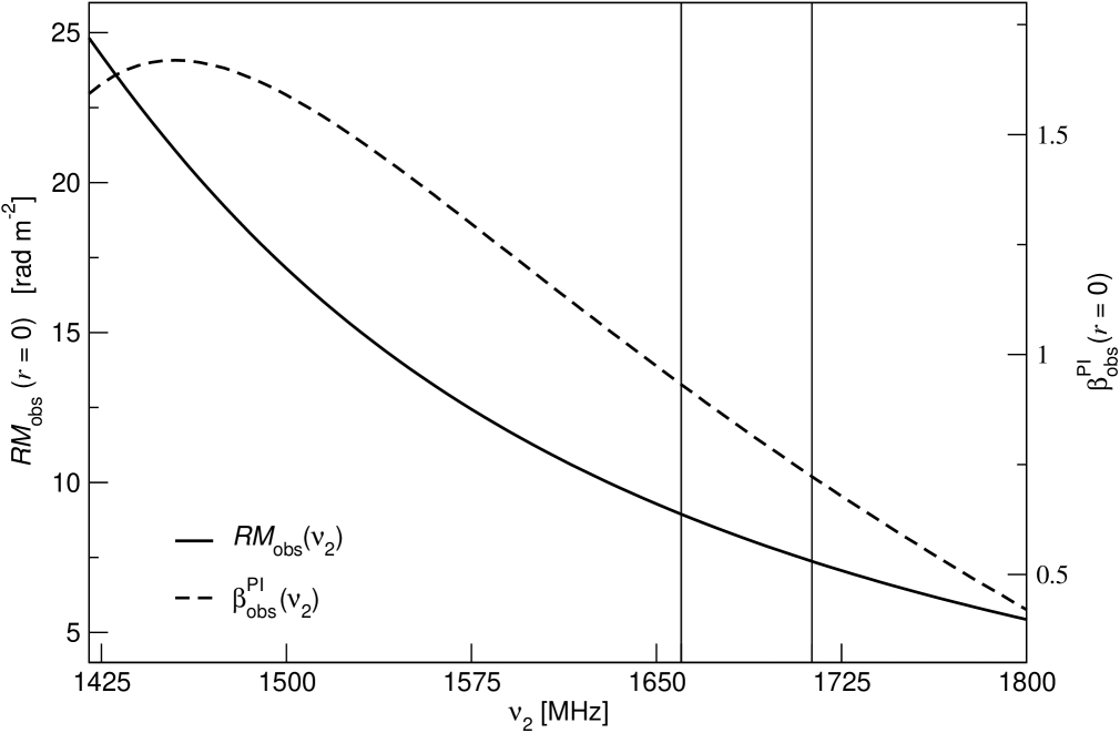
Figure 5: The plot shows two of the modeled observables for object d at frequencies between $1410$ MHz and $1800$ MHz. The observable rotation measure $RM_{\mathrm{obs}}$ (solid), as well as the observable spectral index $\beta^{\mathrm{PI}}_{\mathrm{obs}}$ (dashed) are shown as a function of the second observing frequency for $r=0$ relative to 1408 MHz. Vertical lines mark the two $\lambda\,18\,\mbox{cm}$ frequencies ($1660$ MHz and $1713$ MHz) used in this paper.

4.4 Notes on the model

1. The $PA$–$PI$ diagram contains all observed pixels in the field of the Faraday screen as outlined in Fig. 5. This also holds for the resulting $PA$–$PI$ relation.

2. Towards a Faraday screen the observed $RM_{\mathrm{obs}}$ differs from its intrinsic $RM_{\mathrm{int}}$ depending on the amount of foreground polarization adding to the rotated background polarization. $RM_{\mathrm{obs}}$ depends on the two frequencies ($\nu_{\mathrm{1}},\nu_{\mathrm{2}}$) used for its determination as illustrated in Fig. 5. This also implies no $\lambda^{2}$ dependence of the observed polarization angles in the direction of Faraday screens. Figure 5 shows for object d how $RM_{\mathrm{obs}}$ and spectral index of $PI$ depend on the second observing frequency $\nu_{\mathrm{2}}$, while $\nu_{\mathrm{1}}$ is always 1408 MHz.

4.5 Application of the model

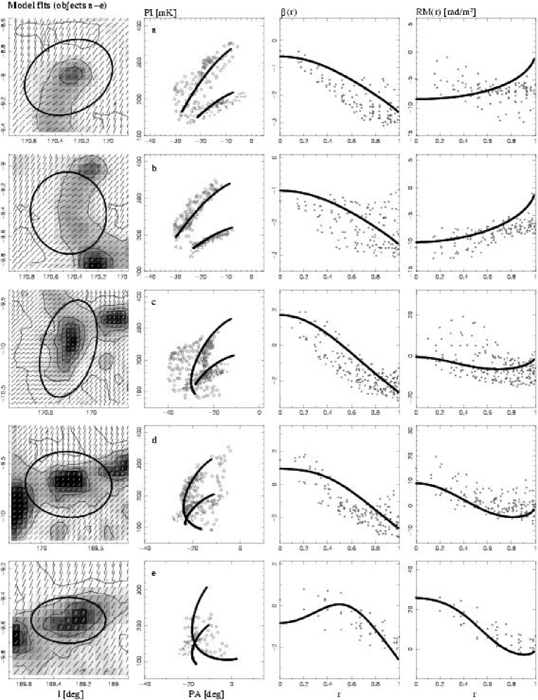
Figure 6: From left to right are shown: The map of $\beta^{\mathrm{PI}}_{\mathrm{obs}}$ in Galactic coordinates with the ellipse marking the size of the Faraday screen, the $PA$–$PI$ plot for 1408 MHz (circles) and $1660$ MHz (crosses), the observed spectral index of the polarized intensity $\beta^{\mathrm{PI}}_{\mathrm{obs}}$, as well as the observed rotation measure $RM_{\mathrm{obs}}$ versus radius $r$. Thick lines indicate the modeled values. Each row refers to a Faraday screen listed in Table 1 and labeled from a to i.

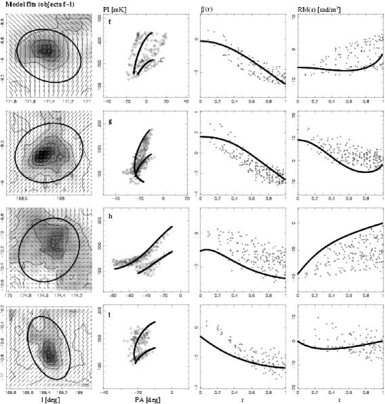
Figure 6: continued

Table 2: Best–fit parameters of our model fits at 1408 MHz for the Faraday screens listed in Table 1

Object	$PI_{\mathrm{fore}}$ [mK]	$PA_{\mathrm{fore}}$ [°]	$PI_{\mathrm{back}}$ [mK]	$PA_{\mathrm{back}}$ [°]	$RM_{\mathrm{0}}$ [rad m-2]	$DP_{\mathrm{0}}$
a	186	3	179	$-$13	$-$18	1
b	172	0	183	$-$10	$-$18	1
c	196	$-$6	145	$-$11	$-$27.5	1
d	200	$-$5	132	$-$13	$-$28	0.9
e	224	$-$2	120	$-$19	$-$29.5	1
f	202	9	138	11	$-$25.5	1
g	170	$-$3	124	$-$13	$-$27.5	0.9
h	82	6	212	$-$15	$-$25	0.9
i	172	$-$6	92	$-$17	$-$22	1

For the nine objects identified as minima in the $\lambda\,21\,\mbox{cm}$ polarized intensities shown in Figs. 2a and b, which also show unusually high $\beta^{\mathrm{PI}}_{\mathrm{obs}}$ as seen from Fig. 2c, we used the following algorithm to apply our Faraday screen model and find the best-fit parameters:

We start by defining the center of the Faraday screen from the $\beta^{\mathrm{PI}}_{\mathrm{obs}}$ map for each object and estimate radius and ellipticity by eye. This is shown in the left panel of Fig. 6.

For normalized radii $r\geq 1$ no Faraday effects are present and the superposition of the foreground and the background model component must agree with the observed polarization. However, in this case Faraday screens may partly overlap and influence the offset polarization.

With the boundary condition that the model must correctly reproduce the observed polarization at $r=1$, four parameters need to be fitted where we allow variations within a reasonable range. These limits are: $50\leavevmode\nobreak\ \mbox{mK}\leq PI\leq 500$ mK for the foreground and the background polarized intensity, $0\leq DP_{\mathrm{0}}\leq 1$ and $-70\leavevmode\nobreak\ \mbox{\hbox{rad$\,$m${}^{-2}$}}\leq RM_{\mathrm{0}}\leq 70$ rad m^-2.

Figure 6 shows the $\beta^{\mathrm{PI}}_{\mathrm{obs}}$ maps, as well as $\beta^{\mathrm{PI}}_{\mathrm{obs}}$ and $RM_{\mathrm{obs}}$ versus radius $r$, and the model fits for the nine Faraday screens listed in Table 1. All the pixels of a Faraday screen located within the ellipse shown in the left-hand panels of Fig. 6 are displayed in the $PA$–$PI$ diagram. We calculated the observed spectral index and $RM$ using the 1408 MHz and $1660$ MHz data. The $1713\,$MHz data were used to check the model parameters for consistency.

In order to estimate how sensitive the model is to systematic effects on the calibration of the large-scale emission of the $\lambda\,18\,\mbox{cm}$ data, we re-calibrated the data for different spectral indices and $RM$s for the large-scale polarized emission ($\beta^{\mathrm{PI}}_{\mathrm{cal}}=-2.7\pm 0.3$ and $RM_{\mathrm{cal}}=0\pm 5$ rad m^-2). Subsequent model fitting showed that the best–fit parameters changed as follows: $\Delta PI_{\mathrm{fore}}$, respectively $\Delta PI_{\mathrm{back}}$ by about $\pm 3$ mK, $\Delta PA_{\mathrm{fore}}$ and $\Delta PA_{\mathrm{back}}$ by about $\pm 5$°, $RM_{\mathrm{0}}$ by about $\pm 5$ rad m^-2. $DP_{\mathrm{0}}$ remained unchanged.

It is also interesting to compare the results from our model based on the large-scale adjustment of the Effelsberg polarization data by the DRAO 1.41 GHz survey presented in this paper with those based on the quite limited Dwingeloo data, which were previously used by Wolleben (woll (2001)) and Wolleben & Reich (woll2 (2004)). For the case of the Taurus region the Dwingeloo-derived corrections leaves the Effelsberg Stokes $U$ data unchanged and gives a 138 mK offset at 1.4 GHz for the Stokes $Q$ map. When comparing the Dwingeloo and DRAO polarization intensity scales a difference of 15% was found in the sense that the Dwingeloo intensities are too high (Wolleben et al., in prep.). In addition the DRAO $U$ and $Q$ maps show some gradients or warping across the field due to their better sampling compared to the Dwingeloo data. Running the same model fitting we get the following differences for the average of all clouds analyzed: $\Delta PI_{\mathrm{fore}}$, respectively $\Delta PI_{\mathrm{back}}$, by about $-25$ mK and $-12$ mk. $\Delta PA_{\mathrm{fore}}$ and $\Delta PA_{\mathrm{back}}$ by about $0$° or $-3$°, $RM_{\mathrm{0}}$ by about $-4.3$ rad m^-2 and $DP_{\mathrm{0}}$ = 1 stays unchanged.

Although it is essential to take the large-scale polarized intensities for the analysis of Faraday screens into account, their uncertainties do not change the qualitative results and the quantitative errors are moderate. The model results for the intrinsic $RM_{\mathrm{0}}$ of the Faraday screens vary within about 20% and allow a conclusive physical interpretation.

5 Analysis and interpretation

The parameters for each object we obtained from our model fits are shown in Table 2. At a frequency of 1408 MHz, the mean values for the emission component in front of the screen is $\overline{PI}_{\mathrm{fore}}=175\pm 40$ mK and $\overline{PA}_{\mathrm{fore}}=-1\pm 5$°. The background yields $\overline{PI}_{\mathrm{back}}=142\pm 37$ mK and $\overline{PA}_{\mathrm{back}}=-11\pm 9\degr$ to the observable polarization. The intrinsic rotation measures of the Faraday screens average to $RM_{\mathrm{0}}=(-25\pm 4)$ rad m^-2. All Faraday screens can be explained with only a small degree of depolarization or none at all.

In the following discussion, the spatial coincidence of polarization minima with the molecular cloud will be interpreted as a strong hint that the Faraday effects, which give rise to the polarization feature, are associated with the molecular cloud. Therefore the distance to the Faraday screens is $140$ pc, the same as it is for the molecular cloud.

Our results show that the background component in most cases is smaller than the foreground emission. This is an unexpected result since the foreground emission originates within only $140$ pc. At a Galactic latitude of about $-10\degr$ the $z$ distance is about $24$ pc and the emission contributing to the background should originate within several kpc. This may indicate that the background layer consists of several superposing emission layers. The longer the line-of-sight the more likely are changes in the Galactic magnetic field direction and/or Faraday rotation within the ISM. This means that depolarization effects increase with the line-of-sight and the observed polarized intensity decreases. The fit-results seem to reflects this.

At a distance of about $140$ pc of the molecular clouds the size of the Faraday screens is of the order of $2$ pc, when spherical symmetry is assumed. Intrinsic $RM_{\mathrm{0}}$ values of up to $-25$ rad m^-2 require an excessive thermal electron density or an excessive regular magnetic field component along the line-of-sight, when compared to average Galactic values. Since $RM$ is the product of both quantities, further constrains are required to derive the appropriate numbers. We have checked available H$\alpha$ data from the ”full-sky H-alpha map” (Finkbeiner haref (2003)), which do not show any related emission ($1\sigma$ detection level of $0.52$ Rayleigh) and constrain $n_{\mathrm{e}}$ to less than $0.8$ cm^-3 for thermal electrons from ionized hydrogen. Upper limits from thermal radio emission give $n_{\mathrm{e}}\leq 2$ cm^-3. With an upper limit of $0.8$ cm^-3 for the thermal electron density $n_{\mathrm{e}}$, a regular magnetic field strength exceeding $20\leavevmode\nobreak\ \mu$G within the Faraday screens along the line-of-sight is needed.

Is the existence of such enhanced localized magnetic field structures in agreement with the observations? While magnetic fields directed towards us will not enhance the total intensity synchrotron emission, similar magnetic field enhancements should also exist in orthogonal directions. We can roughly calculate the expected fluctuations of the Galactic background emission. Let us assume a magnetic field with an orthogonal component of $3\leavevmode\nobreak\ \mu$G extending for $1$ kpc along the line-of-sight and giving about $1$ K brightness temperature, which is a typical value at medium Galactic latitudes at $1.4$ GHz. A magnetic field enhancement of $20\leavevmode\nobreak\ \mu$G over $2$ pc, keeping the relativistic electron density constant, gives about $50$ mK for a temperature spectral index of $\beta=-2.7$. Such magnetic bubbles will cause fluctuations of a few times the confusion limit, which is about $15$ mK T_B for the Effelsberg telescope at $1.4$ GHz. Such fluctuations are quite difficult to identify in practice, and we conclude that the existence of local magnetic field enhancements over size scales of a few parsec is in agreement with the observations. Bubbles with field strength exceeding about $30\leavevmode\nobreak\ \mu$G or $5$ pc in size, however, cause total intensity enhancements of the order of $150$ mK T_B. Such structures should be clearly detectable on available radio maps and therefore are unlikely to exist in large numbers.

5.1 The origin of Faraday screens

Although the origin of the Faraday screens discussed here is not clear, we comment on a number of known processes which might be able to cause an enhancement of n_e and/or the B-field.

5.1.1 Ionization in a PDR

In a photodissociation region (PDR) the physical and chemical properties of the interstellar medium are dominated by UV radiation. This is certainly the case for an O,B star ionizing its surroundings, but even the mean interstellar radiation field can give rise to PDRs. Most of the atomic and molecular gas in our Galaxy is exposed to a far-ultraviolet flux and therefore PDRs are expected to be quite common (see Hollenbach & Tielens 1995).

Models and observations of PDRs show that with increasing extinction $A_{\mathrm{V}}$ the chemistry changes from ionized hydrogen at the surface to neutral and finally to molecular hydrogen inside the cloud. In a similar sequence carbon exists as $\@element{\mathrm{C}}$⁺ in the outer region and in form of $\@element{\mathrm{C}}$ and $\@element{\mathrm{CO}}$ inside. According to these models there is a thin layer in the cloud where the ionization of carbon becomes the main source for electrons, while the hydrogen-ionizing photons are already absorbed.

From Fig. 3b we roughly estimate an excess reddening at the positions of the Faraday screens of $E_{\mathrm{B-V}}\leq 0.5\,$mag. Using the usual gas–to–dust relation $N({H\textsc{i}}+\@element[2]{\mathrm{H}})/E_{\mathrm{B-V}}=5.8\times 10^{21}\leavevmode\nobreak\ \mbox{cm}^{-2}\,\mbox{mag}^{-1}$ (Bohlin et al. bohlin (1978)), the total neutral hydrogen density amounts to $n\leq 470\leavevmode\nobreak\ \mbox{cm}^{-3}$ for the size of the Faraday screens of $2$ pc.

Several authors have derived a C/H ratio of about $10^{-4}$ to $4\times 10^{-4}$. Variations of C/H associated with the physical conditions of the ISM are expected and investigated by Gnacinski (gnacinski (2000)). His analysis indicates variations of C/H for different fractional abundances of molecular hydrogen $f(\@element[2]{\mathrm{H}})=2N(\@element[2]{\mathrm{H}})/(N({H\textsc{i}})+2N\@element[2]{\mathrm{H}}$. Average values of C/H$\leavevmode\nobreak\ =3.55\times 10^{-4}$ for lines-of-sight with $f(\@element[2]{\mathrm{H}})<10^{-3}$, and C/H$\leavevmode\nobreak\ =1.36\times 10^{-4}$ for $f(\@element[2]{\mathrm{H}})>10^{-3}$ were found. For extinctions of $A_{\mathrm{V}}\approx 3.1\,E_{\mathrm{B-V}}\leq 1.6\,$mag, where we observe the Faraday screens, the PDR model by Hollenbach et al. (hollenbach1991 (1991)) gives $f(\@element[2]{\mathrm{H}})<10^{-3}$. In such a case the complete ionization of carbon will enhance the local electron density $n_{\mathrm{e}}$ by about $0.2$ cm^-3.

This simple estimate shows that a significant part of the thermal electrons in the Faraday screens modeled here may be due to carbon ionization in a PDR. In this PDR scenario two extreme cases are possible: either no ionization of hydrogen takes place and all electrons are from ionized carbon (total $n_{\mathrm{e}}\approx 0.2$ cm^-3) or both elements contribute to a total electron density of $n_{\mathrm{e}}\leq 0.8$ cm^-3(H ii)$+0.2$ cm^-3($\@element{\mathrm{C}}$⁺). With a filling factor of $1$, a magnetic field strength between $15\leavevmode\nobreak\ \mu$G and $77\leavevmode\nobreak\ \mu$G is required to produce a $RM_{\mathrm{0}}$ of $-25$ rad m^-2. Further observations of H$\alpha$ and $\@element{\mathrm{C}}$⁺ emission could constrain these limits.

5.1.2 Ionization by cosmic rays

In clouds with moderate gas densities both photoionization and cosmic-ray ionization could be important. Theoretical values for the resulting ionization are not well known and spatial variations are expected. However, referring to McKee (mckee (1989)) a molecular cloud is primarily ionized by the external UV radiation field. Only about a tenth of the mass is ionized by cosmic rays. Model calculations by Myers & Khersonsky (myers (1995)) show that for gas densities comparable to the ones adopted here, photoionization at the surface of a molecular cloud exceeds the ionization fraction from cosmic rays by a factor of $100$. Here an exposure to an UV photon flux from the mean interstellar radiation field is assumed. Therefore ionization by cosmic rays seems to be unimportant.

5.1.3 Magnetic field enhancement

A $RM$ enhancement results when the B_∥ field gets enhanced. There are a number of possibilities to locally enhance the regular component of the magnetic field in interstellar space. Shock waves from supernova remnants are known to compress the field component perpendicular to their velocity direction. Stellar winds or expanding H ii regions will also have an effect on the ambient interstellar magnetic field. However, there is no indication for the presence of a nearby supernova remnant or a massive hot star with a strong stellar wind in the vicinity of the molecular cloud discussed here. Nevertheless weak shock waves in the interstellar medium without any clear signature may cause some magnetic field compression when they hit a massive molecular cloud. Magnetic fields also get enhanced during the formation process of molecular clouds, although missing excessive synchrotron emission limits the magnetic field strength outside the clouds to values not too different from those in the interstellar space. Zeeman-splitting observations could provide the line-of-sight magnetic field strengths or at least an upper limit for the outer regions of molecular clouds.

6 Local synchrotron emissivity

The local synchrotron emissivity has been previously determined by several authors. Either the low-frequency emission in front of H ii regions was measured or model fits of the Galactic synchrotron emission were made. The Beuermann et al. (beuer (1985)) model gives about $11$ K/kpc for $408$ MHz, which corresponds to about $0.4$ K/kpc at 1408 MHz depending on the local synchrotron spectral index where we assumed $\beta$ = -2.7. The Phillipps et al. (phil (1981)) 408 MHz model of the Galaxy places the Sun near a local minimum. They report even lower values corresponding to less than $0.14$ K/kpc at 1408 MHz. For the case of low-frequency measurements towards optically thick H ii regions as discussed by Fleishman & Tokarev (fleishman (1995)) at 10 MHz and Roger et al. (roger (1999)) at 22 MHz an enhanced local volume synchrotron emissivity is indicated. However, this is largely based on the nearest H ii region $\zeta$-Oph (Sh 27) at $\sim$ 170 pc distance, which shows excessive foreground synchrotron emission as discussed by Roger et al. (roger (1999)). Excluding $\zeta$-Oph, Roger et al. (roger (1999)) report a mean value of 30 K/pc at 22 MHz, which corresponds to $0.9$ to $0.6$ K/kpc at 1408 MHz for $\beta$ of -2.5 or -2.6, respectively.

Our mean polarized emission at 1408 MHz in front of the Taurus molecular cloud is about $0.18$ K, which requires a synchrotron emission of at least $0.24$ K for the maximum possible percentage polarization. The distance to the Taurus cloud is $140$ pc. Assuming the same distance for the Faraday screens, this value corresponds to an emissivity of about $1.7$ K/kpc. Since this is a lower limit set by the maximum possible polarization ($\sim 75$%), the local emissivity is likely significantly higher. Other than for the H ii region $\zeta$-Oph (Sh 27), which is at a similar distance, there is no indication for excessive foreground emission towards the Taurus molecular clouds. However, the local emissivity may depend on direction. This may be investigated by measurements of this kind towards molecular clouds in other areas of sky. In case the local synchrotron emissivity derived towards the Taurus cloud holds for all directions, synchrotron models of the Milky Way (Beuermann et al. beuer (1985); Phillipps et al. phil (1981)) may need modifications. Enhanced local emissivity has a significant effect when modeling the thick disk properties of the Galaxy. The large height of $\sim$5 kpc or more inferred by the Beuermann et al. (beuer (1985)) and Phillipps et al. (phil (1981)) models will be reduced or its emissivity decreases. It should be noted that the modeled Galactic halo extends several kpc above the plane. Such halos are rare and place the Milky Way within a small group of galaxies showing similarly huge halos (e.g. Dumke & Krause dumke (1998)).

7 Conclusions

We have used the Effelsberg telescope for observations of the polarized emission in the Taurus region and added the missing large-scale components by making use of a new DRAO 1.4 GHz polarization survey. We observe minima in polarized intensity along the boundary of a molecular cloud complex located at a distance of $140$ pc. Excessive $RM$s were measured based on 1408, 1660 and 1713 MHz data. The polarization angles do not follow a $\lambda^{2}$ dependence, which indicates the presence of components with different physical properties seen in superposition along the line-of-sight. The observed systematic variation of polarization angles with polarized intensity across the Faraday screens were fitted by a model assuming a constant large-scale foreground and also background emission. The large-scale components at $\lambda\,18\,\mbox{cm}$ were scaled from absolutely calibrated $\lambda\,21\,\mbox{cm}$ data with a spectral index of $\beta^{\mathrm{PI}}_{\mathrm{LS}}=-2.7$ and $RM_{\mathrm{LS}}=0$ rad m^-2. We calculate physical parameters for the magneto–ionic medium at the surface of the molecular clouds, which differ largely from average interstellar values. Since there is no observational evidence for enhanced thermal electron density from available data, an enhanced $B$-field is needed to account for the large $RM_{\mathrm{0}}$ observed. Towards Faraday screens our model predicts significant variations of $RM_{\mathrm{obs}}$ for different frequency intervals (see Fig. 5). Recently published $RM$ maps such as those of Haverkorn et al. (haver2 (2003)), Gaensler et al. (gaens (2001)) and Uyanıker et al. (buIII (2003)) are based on fits assuming a $\lambda^{2}$ dependence of multi-channel data. The fit is often imperfect or impossible. This may be due to limitations in the measurement accuracy. However, the superposition of various components of the magneto–ionic interstellar medium results in deviations from a $\lambda^{2}$ dependence and this should be taken into account when quoting $RM$ values.

From the model fits presented we find quite high values for the foreground synchrotron emissivity in the direction of the Taurus molecular clouds. If this emissivity represents the omnidirectional local emissivity, it is several times larger than previously assumed. This will have consequences for the extent of the large-scale-halo or the thick disk emission of the Galaxy, which will shrink in size or is weaker than previously assumed.

- (1) Beuermann, K., Kanbach, G., & Berkhuijsen, E. M. 1985, A&A, 153, 17
- (2) Bingham, R. G. 1966, MNRAS, 134, 327
- (3) Bohlin, R. C., Savage, B. D., & Drake, J. F. 1978, ApJ, 224, 132
- (4) Brouw, W. N., & Spoelstra, T. A. Th. 1976, A&AS, 26, 129
- (5) Burn, B. J. 1966, MNRAS, 133, 67
- (6) Comez, G. C., Benjamin, R. A., & Cox, D. P. 2001, AJ, 122, 908
- (7) Cordes J. M. & Lazio T. J. W. 2003, astro-ph/0207156
- (8) Dame, T. M., Hartmann, D., & Thaddeus, P. 2001, ApJ, 547, 792
- (9) Dumke, M. & Krause, M. 1998, in ”Lecture Notes in Physics: The Local Bubble and Beyond”, p. 555
- (10) Duncan, A. R., Haynes, R., Jones, K., & Stewart, R. 1997, MNRAS, 291, 279
- (11) Duncan, A. R., Reich, P., Reich, W., & Fürst, E. 1999, A&A, 350, 447
- (12) Finkbeiner, D. P. 2003, ApJS146, 407
- (13) Fleishman, G. D. & Tokarev, Yu. V. 1995, A&A, 293, 565
- (14) Gaensler, B., Dickey, J., McClure-Griffiths, N., Green, A., Wieringa, M., & Haynes, R. 2001, ApJ, 549, 959
- (15) Gray, A., Landecker, T. L., Dewdney, P. E., & Taylor, A. R. 1998, Nature, 393, 660
- (16) Gray, A., Landecker, T. L., Dewdney, P. E., Taylor, A. R., Willis, A. G. & Normandeau, M. 1999, ApJ, 514, 221
- (17) Gnacinski, P. 2000, Acta Astronomica, 50, 133
- (18) Haverkorn, M., Katgert, P., & de Bruyn, A. 2000, A&A, 356, 13
- (19) Haverkorn, M., Katgert, P., & de Bruyn, A. 2003, A&A, 403, 1045
- (20) Hollenbach, D. J., Takahashi, T., & Tielens, A. G. G. M. 1991, ApJ, 377, 192
- (21) Junkes, N., Fürst, E. & Reich, W. 1987, A&AS, 69, 451
- (22) McKee, C. F. 1989, ApJ, 345, 782
- (23) Myers, P. C. & Khersonsky, V. K. 1995, ApJ, 442, 186
- (24) Phillipps, S., Kearsey, S., Osborne, J. L., Haslam, C. G. T., & Stoffel, H. 1981, A&A, 98, 286
- (25) Reich, P. & Reich, W. 1986, A&A, 63, 205
- (26) Reich, P. & Reich, W. 1988, A&A 196, 211
- (27) Roger, R. S, Costain, C. H., Landecker, T. L. & Swerdlyk, C. M. 1999, A&AS, 137, 7
- (28) Schlegel, D. J., Finkbeiner, D. P., & Davis, M. 1998, ApJ, 500, 525
- (29) Sokoloff, D. D., Bykov, A. A., Shukurov, A., Berkhuijsen, E. M., Beck, R., & Poezd, A. D. 1998, MNRAS, 299, 189
- (30) Spoelstra, T. T. Th. 1972, A&A, 21, 61
- (31) Strong, A. W., Moskalenko, I. V., & Reimer, O. 2000, ApJ, 537, 763
- (32) Taylor, J. H. & Cordes, J. M. 1993, ApJ, 411, 674
- (33) Uyanıker,B., Fürst, E., Reich, W., Reich, P. & Wielebinski, R. 1998, A&AS, 132, 401
- (34) Uyanıker, B., Fürst, E., Reich, W., Reich, P. & Wielebinski, R. 1999, A&AS, 138, 31
- (35) Uyanıker, B., Landecker, T. L., Gray, A. D. & Kothes, R. 2003, ApJ, 585, 785
- (36) Wieringa, M., de Bruyn, A., Jansen, D., Brouw, W., & Katgert, P. 1993, A&A 268, 215
- (37) Wolleben, M., 2001 Diploma Thesis, Bonn University
- (38) Wolleben, M., Landecker, T. L., Reich, W. & Wielebinski, R. 2004, in ”The Magnetized Interstellar Medium”, Proceedings of the conference, eds. B. Uyanıker, W. Reich & R. Wielebinski, Copernicus GmbH, p. 51
- (39) Wolleben, M. & Reich, W. 2004, in ”The Magnetized Interstellar Medium”, Proceedings of the conference, eds. B. Uyanıker, W. Reich & R. Wielebinski, Copernicus GmbH, p. 99