Determination of confusion noise for far-infrared measurements

We present a detailed assessment of the far-infrared confusion noise imposed on measurements with the ISOPHOT far-infrared detectors and cameras aboard the ISO satellite. We provide confusion noise values for all measurement configurations and observing modes of ISOPHOT in the 90 $\mu$m $\leq$ $\lambda$ $\leq$ 200 $\mu$m wavelength range. Based on these results we also give estimates for cirrus confusion noise levels at the resolution limits of current and future instruments of infrared space telescopes: Spitzer/MIPS, ASTRO-F/FIS and Herschel/PACS.

1 Introduction

Confusion noise is a major limitation in sensitivity and photometric accuracy for the measurements performed with the far-infrared (FIR) filters/detectors of the ISOPHOT instrument (Lemke et al., 1996), on-board the Infrared Space Observatory (ISO, Kessler et al., 1996). As was shown by Kiss et al. (2001, hereafter Paper I) measurements in the long-wavelength filters of the C100 camera (90 and 100 $\mu$m) were affected roughly equally by confusion and instrument noise and measurements with the C200 detector were confusion noise limited. In Paper I we provided estimates of the sky confusion noise – the sum of cirrus confusion noise and fluctuations of the cosmic far-infrared background – for a special measurement configuration (one target position bracketed by two reference positions, single pixel apertures of the ISOPHOT C100 and C200 cameras) and for four ISOPHOT filters. However, it is desirable to investigate the dependence of the confusion noise on all actual measurement configurations. This is a fundamental aspect in the scientific validation and interpretation of FIR ISOPHOT measurements.

Confusion noise predictions for future/current space missions working in the far-infrared usually consider the fluctuations due to the cosmic far-infrared background (CFIRB) only (see e.g. Dole et al., 2003, for Spitzer/MIPS, Jeong et al., 2003, for ASTRO-F/FIS and Negrello et al., 2004, for Spitzer/MIPS). For deep cosmological surveys the cirrus contribution can be minimized by a careful selection of fields with low Galactic emission. However, most of the FIR sky is heavily affected by this phenomenon.

The strength of the cirrus confusion noise is believed to decrease rapidly with improving spatial resolution (see e.g. Gautier et al., 1992; Miville-Deschênes et al., 2002, 2003; Ingalls et al., 2004). According to the formula given by Helou & Beichman (1990), the cirrus confusion noise scales as ($\lambda/D$)^2.5 with $\lambda$ being the wavelength of the observation and $D$ the diameter of the telescope primary mirror. In this respect the 3.5 m Herschel Space Telescope will be superior to other cyrogenic space missions like ISO, ASTRO-F or Spitzer with primary mirror diameters D $<$ 1m. Although the structure of the Galactic cirrus may change below the ISOPHOT resolution limit, our detailed confusion noise study offers the possibility to make predictions for other FIR space telescopes, for the first time based on observations in the 170 $\mu$m range.

In this paper we present a detailed analysis of the confusion noise for ISOPHOT measurements performed with the P3, C100 and C200 detectors in various measurement configurations offered by the ISOPHOT Astronomical Observation Templates (see the ISOPHOT Handbook, Laureijs et al., 2003, for an overview). Based on these results we provide predictions for the achievable photometric accuracy (cirrus confusion noise at the resolution limit) for the Spitzer/MIPS, ASTRO-F/FIS and Herschel/PACS instruments.

2 ISOPHOT instrumental set-up and observational parameters

2.1 Apertures, filters and detector arrays

Since the strength of the confusion noise is highly wavelength dependent (see Paper I), we considered only those ISOPHOT filters, where the confusion noise is at least as strong as the typical value of the instrument noise. These are the filters with central wavelengths $\lambda$ $\geq$ 90 $\mu$m. Some filters lack the required number of appropriate maps, therefore we restricted our analysis to the following detector/filter combinations: C100: 90 and 100 $\mu$m, C200: 170 and 200 $\mu$m (see the ISOPHOT Handbook, Laureijs et al., 2003). Confusion noise analysis has been performed for single pixels and for the whole detector array field-of-view as well. This is necessary, because for some measurement modes the photometric flux is derived from the summed-up fluxes of the array, e.g. for C200 staring, where the source is centered on the common corner of the four detector pixels. In the case of single pixels the size of the target/reference apertures are equal to 46″$\times$46″and 92″$\times$92″for the C100 and C200 camera, respectively. In the case of the full arrays the size of the target/reference apertures are equal to 138″$\times$138″ [3$\times$3 array] and 184″$\times$184″ [2$\times$2 array], respectively. Although there were no suitable ”maps” for the P3 detector – 100 $\mu$m filter combination, this was modeled with the help of maps obtained by the C100 camera in its 100 $\mu$m filter. The system responses of both filters are quite similar (see Laureijs et al., 2003, Appendix A). Five model apertures were constructed using the C100 detector pixel granulation, and corresponding to the 79″, 99″, 120″  and 180″  circular and to the 127″$\times$127″  rectangular apertures. These model ”apertures” were generated by 6$\times$6 pixel matrices on the C100 maps, with weights for each pixel suitably set according to the theoretical footprint value of this pixel relative to the centre of the 100 $\mu$m point-spread function (PSF).

2.2 Covered observing modes

A detailed description of ISOPHOT’s observing modes (AOT = Astronomical Observing Template) can be found in the ISOPHOT Handbook (Laureijs et al., 2003). Below we summarize the essentials features for the derivation of the sky noise. Table 1 contains a traceability matrix of applicable configurations per AOT.

ISOPHOT AOT	submode	detector	aperture	number of	separation
				reference positions	target–reference
PHT 03	staring	P3	79″–180″	1	1$\aas@@fstack{\prime}$5–10′
	chopping	P3	79″–180″	1–2	90″–180″
PHT 05	staring	P3	79″–180″	1	1$\aas@@fstack{\prime}$5–10′
PHT 17/18/19	staring	P3	79″–180″	$\geq$1	1$\aas@@fstack{\prime}$5–1$\aas@@fstack{\circ}$5
PHT 22	staring	C100	138″$\times$138″	1	2$\aas@@fstack{\prime}$5–10′
	staring	C200	184″$\times$184″	1	3′–10′
	chopping	C100	46″$\times$46″	1–2	135″–180″
	chopping	C200	184″$\times$184″	1	180″
	mini-map (3$\times$3)	C100	46″$\times$46″	24	46″–130″
	mini-map (2$\times$2)	C200	92″$\times$92″	8	92″–130″
PHT 25	staring	C100	138″$\times$138″	1	2$\aas@@fstack{\prime}$5–10′
	staring	C200	184″$\times$184″	1	3′–10′
PHT 32	chopping oversampled	C100	46″$\times$46″  or 138″$\times$138″	$\geq$1	46″–138″
	chopping oversampled	C200	92″$\times$92″  or 184″$\times$184″	$\geq$1	92″–184″
PHT 37/38/39	staring	C200	184″$\times$184″	$\geq$1	3′–1$\aas@@fstack{\circ}$5

Table 1: Traceability matrix for the configurations of the investigated C100, C200 and P3 Astronomical Observing Templates

2.2.1 Staring

Staring observations were mainly performed as on-off measurements. The on-off distance was freely selectable, but was in most cases a few arcminutes. There was the possibility of executing a sparse map including several reference positions to any of several target positions. Staring observations are compatible with chopping measurements (rectangular or triangular, depending on the number of reference positions) in our analysis.

2.2.2 Chopping

Chopping observations could be performed with:

• one target and one reference position (rectangular chopping, see Figs. 1a–c). Chopper throws had to be chosen in the range of 90″ $\leq$ $\theta$ $\leq$ 180″(see Table 1).

• one target and two reference positions (triangular and sawtooth chopping, see Fig. 1a–c). Since we do not consider any dependence on the direction of the chopper throw relative to the target, sawtooth and triangular chopping are equivalent in our analysis and are represented by triangular chopping. Typical chopper throws are listed in Table 1.

2.2.3 Mapping

Confusion noise on maps may be determined in many ways, depending on the point-source flux extraction method. This can be e.g. similar to some kind of chopping (see above) using single detector pixels as measuring apertures. A typical and effective way is the aperture photometry, using a single detector pixel or apertures as target aperture and an annulus of pixels placed at a specific distance as reference aperture (see Fig. 1d).

2.2.4 Mini-maps

Mini-maps represented a special observing mode which was basically used for observing point sources with high on-source and background redundancy. In mini-map mode the detector (C100 or C200 cameras) moved ’around’ the source in a way that the source was centered in each detector pixel once during the measurement (see Figs. 1e and f for a schematic representation). The confusion noise was calculated according to the steps of the detector motion around a (hypothetic) source considering the detector pixel with the source centered in as target and the other pixels as reference apertures. All pixels were assumed to have equal sensitivities.

2.2.5 Oversampled maps (P32)

Oversampled maps were performed on a regular grid, composed of a series of overlapping parallel scans in the spacecraft y-axis direction. The chopper was used for oversampling between individual spacecraft positions along the scan line. The same celestial position was observed during several raster pointings allowing for elimination of temporal changes in detector response. Oversamping factors down to 1/3 of the C100 and C200 detector pixel size (15″  and 30″, respectively) were allowed, therefore the internal pixel size of oversampled maps is smaller than that of the maps in our database. However, the final photometry in an oversampled map can be performed in a similar way as in the case of P22 staring raster maps (see Sect. 2.2.3). In this case an aperture size corresponding to the ones in our sample (Tables 2–5) should be chosen (e.g. C100 pixel or full detector array apertures), i.e. adding up flux values of the small map pixels.

3 Confusion noise analysis

3.1 ISOPHOT maps

Our database was built from the final maps produced for Paper I. Therefore we refer to this paper for a detailed description of the data reduction. In summary, the data reduction comprised the following main steps:

• basic data analysis with PIA V9.0 (Gabriel et al., 1997) from raw data (integration ramps, ERD) to surface brightness calibrated maps (AAP);

• flat-fielding using first-quartile normalisation;

• subtraction of the Zodiacal Light emission;

• calculation of the instrument noise.

3.2 Derivation of the confusion noise

The confusion noise of a far-infrared map is characterized by the structure function of k^thorder (see e.g. Gautier et al., 1992; Herbstmeier et al., 1998, for an introduction):

$$S(\underline{\theta},k)=\Bigg{\langle}\Bigg{|}B(\underline{x})-{1\over{k}}{\cdot}\sum_{k}B({\underline{{x}}}+{\underline{\theta}_{k}}){\Bigg{|}}^{2}{\Bigg{\rangle}}_{\underline{{x}}}$$ (1)

where $B$ is the measured sky brightness, $\underline{{x}}$ is the location of the target, $k$ is the number of reference apertures, $\underline{\theta}_{k}$ is the separation vector of the target and the $k^{th}$ reference aperture and the average is taken in spatial coordinates over the whole map. $\underline{\theta}_{k}$-s are determined by the actual measurement configuration. Measurement configurations investigated in this paper are illustrated in Fig. 1.

             
                          
                                                 

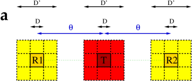
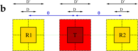
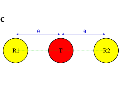
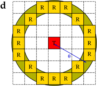
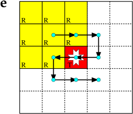
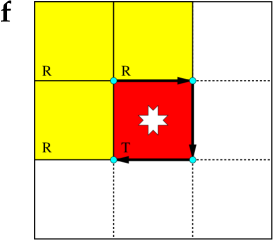
Figure 1: Measurement configurations investigated in our analysis. Target and reference apertures are represented by ”T” and ”R” flags, respectively. In our analysis an aperture can be a single detector pixel (P3, C100, C200) or a full detector-array (C100 or C200) as well. (a) C100 chopping configurations. For rectangular chopping only one reference aperture (R1) and the target aperture (T) is used. For triangular chopping both R1 and R2 reference apertures are applied. Both the target and reference apertures can be single detector pixels ($D$) or full detector arrays ($D^{\prime}$). (b) The same as (a) but for the C200 detector; (c) The same as (a) but for the P3 detector. The P3 detector was mainly used in combination with circular apertures. (d) Circular (annular) aperture at $\theta$ distance around the target aperture. The width of the annulus equals the diameter of the target aperture. In practice the annular reference aperture is realized by a combination of map detector pixels as shown in the figure; (e) Schematic view of the C100 detector mini-map mode (mini-map with 3$\times$3 raster steps). Raster pointings are indicated by the blue dots. The target and reference apertures for the first raster pointing are highlighted in colour; (f) Schematic view of the C200 detector mini-map mode (mini-map with 2$\times$2 raster steps, see C100 description)

The structure noise due to the fluctuations of the sky brightness and instrument noise, $N_{str}$, is defined as:

$$N_{str}(\theta,k)=\sqrt{S(\theta,k)}\times\Omega$$ (2)

where $\Omega$ is the solid angle of the measuring aperture. As shown in Paper I, the relationship between the confusion noise and the instrument noise is:

$$N_{str}^{2}=N^{2}+2N_{inst}^{2}$$ (3)

where $N$ is the real sky confusion noise and $N_{inst}$ is the instrument noise characteristic of a specific far-infrared map. We calculated $N$ using the steps (Eqs. 1–3) described above for specific measurement configurations.

The final confusion noise values were correlated with the average surface brightness of the fields, and this relationship was fitted by a 3-parameter equation (see Paper I):

$$\rm{{N(\underline{\theta},k,\lambda)}\over{1\,mJy}}=C_{0}(\underline{\theta},k,{\lambda})+C_{1}(\underline{\theta},k,\lambda){\cdot}{\bigg{\langle}{{B}\over{1\,MJy\,sr^{-1}}}\bigg{\rangle}}^{\eta(\underline{\theta},k,{\lambda})}$$ (4)

The $C_{0}$, $C_{1}$ and $\eta$ parameters are all functions of the number ($k$) and configuration ($\underline{\theta}$) of reference apertures and the wavelength $\lambda$ of the observation. Note that this confusion noise is the superposition of extragalactic background and cirrus confusion noise.

3.3 Parameter fitting

The C₀, C₁ and $\eta$ coefficients were determined by using a routine based on standard IDL functions. The routine used the Levenberg-Marquardt technique (Press et al., 1992) to solve the least-squares problem.

To perform a completely successful fit for a specific filter/configuration combination, it is necessary to have data points in the whole surface brightness range. Due to the lack of faint fields observed in the C100 100 $\mu$m and C200 200 $\mu$m filters the C₀ parameters for these filters cannot be fitted properly. Therefore conversions of C₀ coefficients have been applied from C100 90 $\mu$m to 100 $\mu$m and from C200 170 $\mu$m to 200 $\mu$m, as described in Sect. 3.4.

C₀ coefficients for the various P3 apertures were determined by simulated confusion noise measurements on synthetic maps with Poissonian brightness-distribution. In these simulated maps the brightness-scaling was arbitrary, and only the confusion noise ratio of a single (C100) pixel to a simulated P3 aperture was calculated for a specific configuration. Then these ratios were applied to the C₀ values of the appropriate configurations in Table 3 to obtain the C₀ coefficients for P3 apertures.

3.4 Coefficients for non-investigated filters

For some other filters, which are similary strongly affected by confusion noise (C100: 105 $\mu$m, C200: 120, 150 and 180 $\mu$m) the number of available maps was too small to perform the investigation as above. For these filters we use transformed coefficients C₀, C₁ and $\eta$ of the filters investigated. The transformations are done as follows:

• The C₀ and C₁ coefficients of the confusion noise – surface brightness relations reflect the spatial structure of the emission. This is expressed via the spectral index $\alpha$ (Helou & Beichman, 1990; Gautier et al., 1992) introducing a scaling of $(\lambda_{1}/\lambda_{0})^{1-{{1}\over{2}}\alpha}$.

• Since $\alpha\,\approx\,0$ for the extragalactic background, C₀ scales as: C₀($\lambda_{1}$,k,$\theta$) =  C₀($\lambda_{0}$,k,$\theta$)$\times(\lambda_{1}/\lambda_{0})$.

• In Paper II we derived an average cirrus spectral index of $\langle\alpha\rangle$ $\approx$ –3 for all filters investigated there. We assume here that this can be applied to other wavelengths as well. This leads to the scaling: C₁($\lambda_{1}$,k,$\theta$) = C₁($\lambda_{0}$,k,$\theta$) $\times(\lambda_{1}/\lambda_{0})^{2.5}$.

• $\eta$ values show a relatively small scatter, and are independent of the filter or even the detector used. The average values for the 90-100 $\mu$m and for the 170-200 $\mu$m filters (see Tables 2…6) are $\eta_{100}$ =1.44$\pm$0.18 and $\eta_{200}$ =1.58$\pm$0.19, respectively. This implies that either the average values or those of individual configurations can be adopted for predictions at other wavelengths. Since the $\eta$ values of specific configurations may still reflect some individual properties, we apply those directly in the transformations, i.e. $\eta(\lambda_{1}$,k,$\theta)$ = $\eta(\lambda_{0}$,k,$\theta)$.

Figure 2: Demonstration of the accuracy of confusion noise predictions using transformations of the C₀, C₁ and $\eta$ parameters. The relative uncertainty $\Delta{N}/N=|N_{tr}-N_{meas}|/N_{meas}$ is plotted versus surface brightness. $N_{tr}$ is the confusion noise calculated using transformed C₀, C₁ and $\eta$ parameters and $N_{meas}$ is the confusion noise calculated using parameters fitted to measurement data of this specific wavelength. The displayed cases are the 90 to 100 $\mu$m and 170 to 200$\mu$m transformations, respectively. The lower and upper limits of the shaded areas reflect the variations among different measurement configurations.

The usability of these transformed parameters was verified for those pairs of filters for which a sufficient number of measurements was available. For the C100 100 $\mu$m filter a transformation was done from the C100 90 $\mu$m filter and compared with the 100 $\mu$m measurements proper, the same was done for the C200 170 $\mu$m and 200 $\mu$m filter pair. This test was only possible for the C₁ and $\eta$ parameters. Both the C100 100 $\mu$m and C200 200 $\mu$m data bases lack low surface brightness measurements and C₀ had to be derived from the 90 $\mu$m and 170$\mu$m value, respectively. The relative uncertainty $\Delta{N}/N\,=\,|N_{tr}-N_{meas}|/N_{meas}$, was determined, where $N_{tr}$ is the confusion noise using transformed parameters and $N_{meas}$ is the confusion noise using parameters fitted to measurement data. The results for the 90-to-100 $\mu$m and the 170-to-200 $\mu$m transformations are presented in Fig. 2. The fitting of the C₀, C₁ and $\eta$ parameters on the one hand and systematic effects like differences in filter bandwidth, changes in the steepness or flatness of the sky background spectral energy distribution between two filters, etc. on the other hand, introduce uncertainties. Considering these, our tests proved that the conversion scheme can be effectively used to estimate confusion noise for non-investigated filters. Taking into account the dependence of confusion noise on surface brightness and the uncertainty of measuring the latter, even an uncertainty of 50% provides an acceptable range for the confusion noise estimates.

4 Results for ISOPHOT filters

4.1 Tables and data products

ap.	con.	$\theta$	C0	C1	$\eta$
			(mJy)	(mJy)
P	R	92″	10.5$\pm$ 2.3	0.95$\pm$0.11	1.47$\pm$0.31
P	R	138″	8.7$\pm$ 2.5	1.97$\pm$0.26	1.27$\pm$0.26
P	R	184″	8.6$\pm$ 2.7	2.04$\pm$0.26	1.34$\pm$0.26
P	R	230″	8.3$\pm$ 2.8	2.10$\pm$0.28	1.38$\pm$0.26
P	T	92″	9.4$\pm$ 1.9	0.63$\pm$0.10	1.47$\pm$0.33
P	T	138″	7.3$\pm$ 2.0	2.09$\pm$0.30	1.07$\pm$0.24
P	T	184″	7.9$\pm$ 2.0	1.67$\pm$0.19	1.25$\pm$0.26
P	T	230″	6.5$\pm$ 2.0	2.43$\pm$0.42	1.17$\pm$0.24
P	C	92″	8.1$\pm$ 1.8	0.74$\pm$0.14	1.36$\pm$0.30
P	C	138″	6.3$\pm$ 1.8	1.63$\pm$0.28	1.11$\pm$0.25
P	C	184″	6.0$\pm$ 1.7	1.56$\pm$0.15	1.23$\pm$0.26
F	R	92″	25.4$\pm$14.7	9.30$\pm$2.52	1.32$\pm$0.18
F	R	138″	28.4$\pm$19.3	13.27$\pm$3.79	1.33$\pm$0.17
F	R	184″	23.8$\pm$21.4	17.35$\pm$5.10	1.32$\pm$0.16
F	R	230″	17.9$\pm$21.8	20.70$\pm$6.16	1.32$\pm$0.15
F	T	92″	28.6$\pm$10.2	2.58$\pm$0.43	1.33$\pm$0.26
F	T	138″	32.6$\pm$15.7	6.46$\pm$1.42	1.31$\pm$0.18
F	T	184″	30.6$\pm$16.3	8.89$\pm$3.88	1.35$\pm$0.35
F	T	230″	25.5$\pm$18.4	12.59$\pm$6.11	1.30$\pm$0.34

Table 2: Fitted coefficients of Eq. 4 for the C100 camera 90$\mu$m filter. Abbreviations in the table: ”ap.” = aperture: P =  single pixel, F = full array; ”con.” = configuration for sky reference determinaion: R = rectangular chopping (one reference position), T = triangular chopping (two reference positions), C = annular aperture.

ap.	con.	$\theta$	C0	C1	$\eta$
			(mJy)	(mJy)
P	R	92″	11.6$\pm$ 2.5	1.35$\pm$0.71	1.39$\pm$0.11
P	R	138″	9.6$\pm$ 2.8	1.47$\pm$0.67	1.44$\pm$0.12
P	R	184″	9.5$\pm$ 3.0	1.52$\pm$0.72	1.51$\pm$0.13
P	R	230″	9.2$\pm$ 3.1	1.60$\pm$0.75	1.55$\pm$0.15
P	T	92″	10.3$\pm$ 2.1	1.14$\pm$0.69	1.29$\pm$0.08
P	T	138″	8.1$\pm$ 2.2	1.44$\pm$0.70	1.28$\pm$0.12
P	T	184″	8.7$\pm$ 2.3	1.42$\pm$0.70	1.43$\pm$0.12
P	T	230″	7.2$\pm$ 2.2	1.57$\pm$0.75	1.58$\pm$0.14
P	C	92″	9.0$\pm$ 2.0	1.13$\pm$0.60	1.25$\pm$0.08
P	C	138″	7.0$\pm$ 2.0	1.47$\pm$0.70	1.25$\pm$0.12
P	C	184″	6.6$\pm$ 1.9	1.47$\pm$0.71	1.34$\pm$0.13
F	R	92″	28.6$\pm$16.3	6.47$\pm$2.03	1.51$\pm$0.40
F	R	138″	31.6$\pm$21.4	8.26$\pm$2.53	1.55$\pm$0.41
F	R	184″	25.6$\pm$23.7	9.56$\pm$3.34	1.59$\pm$0.42
F	R	230″	19.9$\pm$24.2	10.33$\pm$3.67	1.61$\pm$0.43
F	T	92″	31.9$\pm$11.3	3.42$\pm$0.98	1.43$\pm$0.45
F	T	138″	36.2$\pm$17.5	3.71$\pm$0.57	1.63$\pm$0.70
F	T	184″	34.0$\pm$18.1	7.38$\pm$2.41	1.47$\pm$0.39
F	T	230″	25.8$\pm$20.4	14.03$\pm$4.15	1.31$\pm$0.26

Table 3: Fitted coefficients of Eq. 4 for the 100$\mu$m filter of the C100 detector. C₀ coefficients have been transformed from 90 $\mu$m results (see Sect. 2.5). For the meaning of labels for apertures (ap.) and configurations (con.) see the caption of Table 2.

ap.	con.	$\theta$	C0	C1	$\eta$
			(mJy)	(mJy)
P	R	184″	19.8$\pm$ 5.4	0.94$\pm$0.42	1.86$\pm$0.21
P	R	276″	16.6$\pm$ 6.2	2.27$\pm$0.54	1.71$\pm$0.20
P	R	368″	12.3$\pm$ 6.8	3.74$\pm$0.58	1.61$\pm$0.19
P	R	460″	5.6$\pm$ 7.5	5.87$\pm$0.61	1.54$\pm$0.18
P	T	184″	10.2$\pm$ 4.5	3.01$\pm$0.31	1.47$\pm$0.16
P	T	276″	18.3$\pm$ 7.0	1.61$\pm$0.22	1.66$\pm$0.12
P	T	368″	18.9$\pm$ 6.7	1.58$\pm$0.24	1.70$\pm$0.12
P	T	460″	14.4$\pm$ 7.6	2.06$\pm$0.55	1.66$\pm$0.11
P	C	184″	9.3$\pm$ 6.7	3.37$\pm$1.01	1.46$\pm$0.17
P	C	276″	16.4$\pm$ 8.5	1.83$\pm$0.15	1.65$\pm$0.23
P	C	368″	13.8$\pm$ 6.8	1.21$\pm$0.50	1.72$\pm$0.21
F	R	184″	49.1$\pm$21.0	4.72$\pm$1.15	1.78$\pm$0.21
F	R	276″	40.4$\pm$24.2	10.28$\pm$1.29	1.66$\pm$0.20
F	R	368″	20.7$\pm$28.2	17.56$\pm$1.38	1.57$\pm$0.19
F	R	460″	7.5$\pm$27.8	21.15$\pm$1.41	1.59$\pm$0.19
F	T	184″	51.3$\pm$17.6	1.40$\pm$0.51	1.89$\pm$0.23
F	T	276″	59.2$\pm$32.4	2.01$\pm$0.54	1.93$\pm$0.24
F	T	368″	53.6$\pm$23.9	4.55$\pm$1.17	1.76$\pm$0.22
F	T	460″	36.2$\pm$25.4	9.19$\pm$1.30	1.62$\pm$0.19

Table 4: Fitted coefficients of Eq. 4 for the 170$\mu$m filter of the C200 camera. For the meaning of labels for apertures (ap.) and configurations (con.) see the caption of Table 2.

ap.	con.	$\theta$	C0	C1	$\eta$
			(mJy)	(mJy)
P	R	184″	23.3$\pm$ 6.3	7.81$\pm$2.35	1.42$\pm$0.32
P	R	276″	19.5$\pm$ 7.3	10.03$\pm$3.23	1.46$\pm$0.32
P	R	368″	14.5$\pm$ 8.1	11.05$\pm$3.64	1.48$\pm$0.33
P	R	460″	6.6$\pm$ 8.8	12.34$\pm$4.16	1.49$\pm$0.33
P	T	184″	12.0$\pm$ 5.2	7.17$\pm$2.10	1.30$\pm$0.29
P	T	276″	21.6$\pm$ 8.2	7.95$\pm$2.40	1.40$\pm$0.31
P	T	368″	22.3$\pm$ 7.9	8.22$\pm$2.52	1.45$\pm$0.32
P	T	460″	16.9$\pm$ 8.9	9.75$\pm$3.14	1.47$\pm$0.33
P	C	184″	11.0$\pm$ 7.8	7.75$\pm$2.32	1.26$\pm$0.28
P	C	276″	19.3$\pm$10.0	8.58$\pm$2.65	1.37$\pm$0.30
P	C	368″	16.3$\pm$ 8.0	6.26$\pm$1.76	1.55$\pm$0.34
F	R	184″	57.8$\pm$24.7	18.20$\pm$6.62	1.58$\pm$0.35
F	R	276″	47.6$\pm$28.4	23.71$\pm$8.98	1.61$\pm$0.36
F	R	368″	24.1$\pm$33.2	25.68$\pm$9.84	1.64$\pm$0.37
F	R	460″	8.8$\pm$32.7	24.95$\pm$9.52	1.67$\pm$0.37
F	T	184″	60.4$\pm$20.7	14.07$\pm$4.88	1.46$\pm$0.32
F	T	276″	69.9$\pm$38.1	17.36$\pm$6.26	1.55$\pm$0.34
F	T	368″	63.1$\pm$28.1	18.75$\pm$6.87	1.63$\pm$0.36
F	T	460″	42.6$\pm$29.8	14.78$\pm$5.36	1.74$\pm$0.41

Table 5: Fitted coefficients of Eq. 4 for the 200 $\mu$m filter of the C200 camera. C₀ coefficients have been transformed from the 170 $\mu$m results (see Sect. 2.5). For the meaning of labels for apertures (ap.) and configurations (con.) see the caption of Table 2.

detector	filter	C0	C1	$\eta$
		(mJy)	(mJy)
C100	90 $\mu$m	8.1$\pm$2.0	0.74$\pm$0.18	1.36$\pm$0.09
C100	100 $\mu$m	9.0$\pm$3.1	0.96$\pm$0.24	1.36$\pm$0.10
C200	170 $\mu$m	12.2$\pm$3.5	0.65$\pm$0.12	1.63$\pm$0.32
C200	200 $\mu$m	14.4$\pm$3.8	2.35$\pm$0.98	1.41$\pm$0.19

Table 6: Fitted coefficients of Eq. 4 for the C100/90 $\mu$m, C100/100 $\mu$m, C200/170 $\mu$m, C200/200 $\mu$m detector/filter combinations for the simulated mini-map observing mode. C₀ coefficients for the 100 $\mu$m filter have been transformed from the 90 $\mu$m results, for the 200 $\mu$m filter from the 170 $\mu$m results.

aper.	con.	$\theta$	C0	C1	$\eta$
			(mJy)	(mJy)
79″$\bigcirc$	R	90″	7.8$\pm$1.7	2.25$\pm$0.52	1.15$\pm$0.19
79″$\bigcirc$	T	90″	6.0$\pm$1.2	1.08$\pm$0.19	1.13$\pm$0.15
99″$\bigcirc$	T	90″	9.0$\pm$1.9	0.74$\pm$0.12	1.18$\pm$0.18
79″$\bigcirc$	T	120″	6.0$\pm$1.2	1.93$\pm$0.37	1.10$\pm$0.18
99″$\bigcirc$	R	120″	10.9$\pm$2.3	2.86$\pm$0.27	1.16$\pm$0.19
99″$\bigcirc$	T	120″	9.0$\pm$1.9	1.59$\pm$0.22	1.13$\pm$0.19
120″$\bigcirc$	R	120″	14.0$\pm$3.0	2.46$\pm$0.17	1.17$\pm$0.18
120″$\bigcirc$	T	120″	11.7$\pm$2.4	1.29$\pm$0.11	1.15$\pm$0.17
79″$\bigcirc$	R	180″	7.8$\pm$1.7	3.30$\pm$0.37	1.21$\pm$0.20
99″$\bigcirc$	R	180″	10.9$\pm$2.3	3.37$\pm$0.34	1.18$\pm$0.19
120″$\bigcirc$	R	180″	14.0$\pm$3.0	3.13$\pm$0.26	1.17$\pm$0.18
127″$\square$	R	180″	17.1$\pm$4.2	3.26$\pm$0.51	1.23$\pm$0.21
180″$\bigcirc$	R	180″	24.0$\pm$5.2	2.33$\pm$0.30	1.23$\pm$0.20
120″$\bigcirc$	R	240″	14.0$\pm$3.0	3.61$\pm$0.34	1.18$\pm$0.20

Table 7: Fitted coefficients of Eq. 4 for the simulated P3 detector – aperture combinations in the 100 $\mu$m filter. Coefficients were derived for only those combinations, which were selected for observations .

The fitted C₀, C₁ and $\eta$ parameters for a specific detector / filter / configuration combination are tabulated in Tables 2–7. It should be emphasized that the presented confusion noise values are ’per beam’ and 1$\sigma$ values. They have to be corrected with the appropriate PSF-fraction of the beam when compared with point-source confusion noise values. An example of the functional behaviour of the confusion noise with surface brightness is given in fig. 2 in Paper I.

Due to the surface brightness range of the measurements used in our analysis the predictions with the coefficients in Tables 2–7 are reliable in the 1 $\leq$ $\langle B\rangle$ $\leq$ 100 MJy sr^-1 and in the 1 $\leq$ $\langle B\rangle$ $\leq$ 200 MJy sr^-1 range for the C100/P3 and the C200 detectors, respectively. There are no suitable measurements at high surface brightness and in addition the structure of the FIR emission may change significantly above this level (see Kiss et al., 2003, hereafter Paper II). Therefore we cannot give accurate estimates for very high surface brightness values using our current database.

Based on the results compiled in the tables we constructed all-sky confusion noise maps, one for each detector / filter / configuration combination. Surface brightness values for all positions of our 1° resolution grid were derived from COBE/DIRBE data with the Zodiacal Light contribution removed and interpolated to the ISOPHOT bands, as described in Paper I. The only difference is that the cirrus colour temperature was not fixed to 20 K, but was derived from the COBE/DIRBE 100, 140 and 240 $\mu$m surface brightness values. Due to the in general higher uncertainty a lower weight was given to the 140 $\mu$m band data. The long wavelength baseline of the 100 and 240 $\mu$m bands and the COBE/DIRBE surface brightness accuracies of a few percent provide a final temperature accuracy $\delta$T $\leq$ 0.2 K.

We calculated the confusion noise from these surface brightness values using Eq. 4 and the C₀, C₁ and $\eta$ parameters corresponding to the actual measurement configuration (Tables 2…7). The maps are available in the electronic version of this paper in FITS format. The data format is described in Appendix A.1. One advantage of these maps is that they are based on a homogeneous all-sky surface brightness calibration. In quite a number of cases the determination of the background value from the ISOPHOT measurement itself may be less accurate (e.g. in chopped observations). In this case the confusion noise estimated by using Eq. 4 in combination with the measured background brightness is unreliable. Our all-sky maps provide information on the average confusion noise around the target field, averaged over an area of $\sim$1 deg²,which can be more reliable, if there are no strong gradients in the background brightness over this scale. There are also maps for the filters originally not investigated, with the transformations described in Sect. 3.4 applied.

4.2 Noise performance of various observing modes

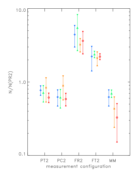
Figure 3: Comparison of the confusion noise values for different observing modes and measurement configurations. The measurement configurations are coded by the labels and the separation $\theta$ is given in detector pixels of the actual detector: PT2 – triangular chopping, pixel aperture, $\theta$ = 2; PC2 – circular aperture (annulus of pixels), $\theta$ = 2; FR2 – rectangular chopping, detector array aperture, $\theta$ = 2; FT2 – triangular chopping, detector array aperture, $\theta$ = 2; MM – mini-map mode. All values are given as ratios with regard to the reference configuration ’PR2’: rectangular chopping, single pixel aperture, $\theta$ = 2. The ISOPHOT filters are marked by the following symbols: diamond: C100 90 $\mu$m; triangle: C100, 100 $\mu$m; asterisk: C200. 170 $\mu$m; circle: C200, 200 $\mu$m; The vertical bars limited by the arrowheads represent the range of ratios for surface brightness values of 2 MJy sr^-1 $\leq$ $\langle$B$\rangle$ $\leq$ 100 MJy sr^-1.

In Fig. 3 we compare the confusion noise values obtained for various observing modes. We have chosen the rectangular chopping with a single pixel aperture and with a separation of $\theta_{min}$ = 2 pixels as reference (denoted ’PR2’). This is compared with the results of other configurations (detailed in the figure caption).

The background determination in mini-map mode turned out to provide the lowest confusion noise in most cases. The second reference position in triangular chopping reduces the confusion noise significantly (by 15–50%) compared to rectangular chopping. Full detector array apertures prove to be 3–5 times more strongly affected by confusion noise than the same configuration with single pixels.

4.3 Noise characterization of individual measurements in the ISO Data Archive

The confusion noise can be a severe limit both for the signal-to-noise and the photometric accuracy of faint sources. Due to the analysis described here it is now possible to determine a robust confusion noise estimate for all FIR ISOPHOT measurements performed with the AOTs listed in Table 1 and which are compact source measurements including background reference positions. From ISO Data Archive (Kessler et al., 2003) Version 7 onward the Data Quality Report of these observations flags the possible cirrus confusion contamination and an associated catalogue file gives the confusion noise numbers calculated both for the measured ISOPHOT and the COBE/DIRBE background values. These can be directly compared with source fluxes extracted from the data products.

5 Cirrus confusion noise predictions for infrared space telescopes

5.1 Simulated maps of cirrus structures

In this analysis we concentrate on the cirrus component of the confusion noise and its scaling between instruments with various spatial resolutions. Here we consider neither the contribution of the extragalactic background nor the impact by any instrumental effect. The main characteristic of the cirrus emission at a specific wavelength is its spatial structure. This is usually described by the spectral index, $\alpha$, of the power spectrum of the image, averaged over annuli (see Paper II for a summary). With this parameter the power spectrum is $P(f)=P_{0}(f/f_{0})^{\alpha}$, where $P(f)$ is the power at the spatial frequency $f$ and $P_{0}$ is the power at the reference spatial frequency $f_{0}$. As was shown in Paper II, $\alpha$ may vary with wavelength and surface brightness. Previous studies (Papers I & II) unraveled the structure of the emission for the scale down to the ISOPHOT resolution. Extrapolations to better spatial resolutions of future space telescopes can be performed using these results and assuming that the general behaviour of the spatial structure remains unchanged for higher spatial frequencies, i.e. the same fractal dimension / the same spectral index is valid.

The correct simulation of the entire cirrus structure of a specific sky area in the Fourier space would demand the reproduction of both the power and phase information. However, in any autocorrelation analysis like the confusion noise calculation, only the Fourier power is important, since the two-dimensional autocorrelation function is related to the two-dimensional power spectrum only:

$$C(\theta)={{1}\over{2\pi}}\int_{0}^{\infty}P(f^{\prime})\,J_{0}(f^{\prime}\theta)\,f^{\prime}\,df^{\prime}$$ (5)

where $P(f^{\prime})$ is the two-dimensional power spectrum, $J_{0}(x)$ is the circular Bessel-function of the 0^th kind and $\theta$ is the angular separation. The confusion noise $N$ is proportional to C($\theta$) or in more complex configurations $N$ is a linear combination of some C($\theta_{i}$)-s. Different FIR instruments sample the power spectrum at different spatial frequencies due to their different resolving power, resulting in different confusion noise levels on the same (cirrus) structure. Only $P_{0}$ depends on the surface brightness $B$ (Gautier et al., 1992). For a power-law type power spectrum the ratio of two power levels at two spatial frequencies is independent of $P_{0}$ and therefore of $B$. If one knows the $P_{0}$–$B$ relation for one specific instrument (e.g. ISOPHOT), it is straightforward to derive a $P$–$B$ relation for another instrument using $P(f)=P_{0}(f/f_{0})^{\alpha}$. This is equivalent with a confusion noise – surface brightness relation for this other instrument.

However, for a specific instrument the size of the detector pixels and the measurement configuration play an important role as well. Because of this complexity the easiest way to compare different instruments is the confusion noise analysis of simulated maps as these would be obtained by these instruments. This is done in the same way as for the real ISOPHOT maps in Sect. 3.

For ISOPHOT we derived the relation between the cirrus confusion noise and the surface brightness of individual fields in Sect. 4. From simulated fractal maps the confusion noise ratios of ISOPHOT and another instrument can be obtained. In this way the cirrus confusion noise of any FIR instrument can be connected to the surface brightness.

To perform the investigation we constructed high-resolution (4096$\times$4096 pixels, 0$\aas@@fstack{\prime\prime}$5 pixel size) synthetic images for a range of spectral index values (–2.0 $\geq$ $\alpha$ $\geq$ –5.0). The generation of the maps is based on the random recursive fractal algorithm by Elmegreen (1997).

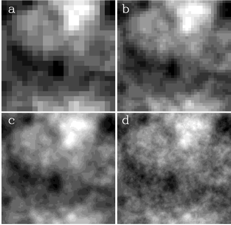
Figure 4: Simulated fractal map with $\alpha$ = –3, as seen with the spatial resolution of various telescopes/instruments. (a) ISOPHOT 170 $\mu$m; (b) ASTRO-F/FIS 170 $\mu$m; (c) Spitzer/MIPS 160 $\mu$m; (d) Herschel/PACS 175 $\mu$m

The high resolution maps were convolved with the beams of the actual telescope/detector/filter combinations and then sampled according to the size of the detector pixels. The Spitzer/MIPS 160$\mu$m point spread function is available at the Spitzer Science Center website. Point spread functions for the Herschel/PACS 110 and 175 $\mu$m simulated measurements were taken from model calculations (Okumura & Longval, 2001). The ASTRO-F/FIS PSFs were calculated theoretically using the latest information on the telescope design (Jeong et al., 2003). The result of this convolution and resampling is shown in Fig. 4.

The confusion noise analysis was performed in the same way as for ISOPHOT observations. The analysis was restricted to the triangular chopping configuration, and the separation $\theta$ was chosen to be equal to the resolution limits of the actual telescope/detector/filter combinations. Since confusion noise is especially important for detection of faint point sources, we provide 1$\sigma$ point source confusion noise values after a correction for the footprint of the instruments, instead of single-pixel (”per beam”) confusion noise values.

5.2 Results

5.2.1 Conversion coefficients:

The main parameters of the investigated instruments and the conversion coefficients are summarized in Table 8. The conversion equation is:

$$N_{R}=R^{PS}\times N_{PHT}$$ (6)

where $N_{PHT}$ and $N_{R}$ are the confusion noise values obtained by ISOPHOT and another instrument for the same map, respectively and $R^{PS}$ is the conversion coefficient. The $R^{PS}$ factor can also be expressed in terms of the C₁ and central point spread function fraction ($f_{psf}$) factors of ISOPHOT and the investigated instrument at their resolution limits:

$$R^{PS}={{C_{1}^{R}(\lambda,\theta_{min}^{R},k,\alpha){\cdot}f_{psf}^{PHT}}\over{C_{1}^{PHT}(\lambda_{ref},\theta_{min}^{PHT},k,\alpha)}{\cdot}f_{psf}^{R}}$$ (7)

These R^PS factors of Table 8 can be compared with the simple telescope resolution scaling ($\lambda/D$)^2.5 (for $\alpha$ = –3) in the Helou & Beichman (1990) formula. For the 85 cm Spitzer telescope R_HB = 4.2$\cdot$10^-1 and for the 3.5 m Herschel telescope R_HB = 1.2$\cdot$10^-2. An example of a graphical comparison is shown in Fig. 5.

instrument	filter	$R^{PS}({\alpha=-2.0})$	$R^{PS}({\alpha=-3.0})$	$R^{PS}({\alpha=-4.0})$	$R^{PS}({\alpha=-5.0})$	res. limit	PHT ref.
ASTRO-F/FIS	170 $\mu$m	4.4$\times$10-1	3.9$\times$10-1	3.5$\times$10-1	3.1$\times$10-1	65$\aas@@fstack{\prime\prime}$5	170 $\mu$m
Spitzer/MIPS	160 $\mu$m	1.6$\times$10-1	1.2$\times$10-1	8.7$\times$10-2	6.5$\times$10-2	46$\aas@@fstack{\prime\prime}$5	170 $\mu$m
Herschel/PACS	110 $\mu$m	3.0$\times$10-2	1.3$\times$10-2	5.3$\times$10-3	2.4$\times$10-3	8$\aas@@fstack{\prime\prime}$5	90 $\mu$m
Herschel/PACS	175 $\mu$m	1.6$\times$10-2	7.4$\times$10-3	3.0$\times$10-3	1.4$\times$10-3	13$\aas@@fstack{\prime\prime}$5	170 $\mu$m

Table 8: Conversion coefficients for point sources between ISOPHOT and the specified instruments for cirrus confusion noise calculations. The columns of the table contain: 1.) Instrument; 2.) Filter; 3.) Ratio of confusion noise values at the resolution limits for a spectral index of $\alpha$ = –2.0; 4.) same for $\alpha$ = –3.0; 5.) same for $\alpha$ = –4.0; 6.) same for $\alpha$ = –5.0; 7.) Resolution limits of the current instrument/filter combination (76″and 143″for the ISOPHOT 90 and 170 $\mu$m filters, respectively); 8.) ISOPHOT reference filter.

5.2.2 All-sky confusion noise maps:

Based on the conversion factors derived above we were able to produce low spatial resolution all-sky cirrus confusion noise prediction maps in a similar way as for the ISOPHOT all-sky confusion noise maps. Surface brightness values were derived from COBE/DIRBE data, following the same scheme as in Sect. 4.1. The confusion noise values of the all-sky maps are calculated for the configuration PT2 (Tables 2 and 4, $\theta$ = 92″ for C100 90 $\mu$m and $\theta$ = 184″ for C200 170 $\mu$m ) The C₀, C₁ and $\eta$ coefficients for this configuration cannot be applied directly, since those resulted from the fits to the total surface brightness, which contains the contribution of the extragalactic background as well. Therefore we fitted parameters using a slightly modified version of Eq. 4:

$$\rm{{N}\over{1\,mJy}}=C_{0}^{*}+C_{1}^{*}{\cdot}{\bigg{\langle}{{B(\lambda)-B_{CFIRB}(\lambda)}\over{1\,MJy\,sr^{-1}}}\bigg{\rangle}}^{\eta^{*}}$$ (8)

$B_{CFIRB}$ is the surface brightness of the cosmic far-infrared background at a specific wavelength (c.f. Pei et al., 1999) and $B-B_{CFIRB}$ = $B_{cirr}$ is the cirrus surface brightness. If $B_{cirr}$ = 0, then $N$ = $C_{0}^{*}$, i.e. the confusion noise is purely due to cosmic infrared background fluctuations. This indicates that $C_{1}^{*}\cdot\langle B_{cirr}\rangle^{\eta^{*}}$ is the pure cirrus confusion noise component. We used these $C_{1}^{*}$ and $\eta^{*}$ values, together with the coefficients in Table 8 for the creation of the all-sky cirrus confusion noise maps. The $C_{0}^{*}$, $C_{1}^{*}$ and ${\eta^{*}}$ parameters are listed in the headers of the FITS files.

Figure 5: Demonstration of the effects of the ISOPHOT–DIRBE photometric transformation and variable spectral index $\alpha$ for the Herschel/PACS 175 $\mu$m filter cirrus confusion noise predicions. Solid line: no DIRBE–ISOPHOT transformation, constant $\alpha$; Dashed line: no DIRBE–ISOPHOT transformation, variable $\alpha$; Dash-dotted line: DIRBE–ISOPHOT conversion applied, constant $\alpha$; Dash-triple-dotted line: DIRBE–ISOPHOT conversion applied, variable $\alpha$. The dotted line shows the prediction according to Helou & Beichman (1990).

There are two other issues which have to be considered in the production of the confusion noise prediction maps:

• Transformation between the COBE/DIRBE and ISOPHOT photometric systems. The all-sky surface brightness maps are in the DIRBE photometric system, while the coefficients are derived in the ISOPHOT system. We used the latest available transformation coefficients based on the comparison of DIRBE surface brightness values and ISOPHOT mini-map background fluxes obtained with PIA V10.0/CALG 7.0 (Moór, 2003, priv. comm.). The transformation equation was:

  $$B_{DIRBE}^{\lambda}=Gain{\times}B_{PHT}^{\lambda}+Offset$$ (9)

  where $B_{DIRBE}^{\lambda}$ and $B_{PHT}^{\lambda}$ are the COBE/DIRBE and ISOPHOT surface brightness values, respectively. The transformation coefficients (Gain and Offset) for different filters are summarized in Table 9.

  filter	Offset	Gain
  	(MJysr-1)
  90 $\mu$m	–1.65$\pm$0.06	1.00$\pm$0.01
  100 $\mu$m	0.09$\pm$0.09	0.85$\pm$0.02
  120 $\mu$m	0.62$\pm$0.28	0.95$\pm$0.07
  150 $\mu$m	0.28$\pm$0.15	1.02$\pm$0.03
  170 $\mu$m	0.09$\pm$0.09	1.06$\pm$0.02
  180 $\mu$m	–0.50$\pm$0.32	1.15$\pm$0.09
  200 $\mu$m	0.95$\pm$0.17	0.97$\pm$0.03

  Table 9: Transformation coefficients between the ISOPHOT and the DIRBE photometric systems, according to Eq. 9.

• Constant or variable spectral index ($\alpha$). As shown in Paper II, the spectral index $\alpha$ depends on the surface brightness of the observed fields and on the observational wavelength. The surface brightness dependence of $\alpha$ is approximated by:

  $$\rm\alpha\,=\,A_{1}\,\,{\times}\,\,log_{10}\bigg{\langle}{{B-B_{CFIRB}}\over{1\,MJy\,sr^{-1}}}\bigg{\rangle}\,\,+A_{0}$$ (10)

  where B is the average surface brightness of the field after the removal of the Zodiacal Light contribution and B_CFIRB is the surface brightness of the cosmic far-infrared background. The coefficients are: A₀ = –1.67$\pm$0.47 and A₁ = –1.57$\pm$0.38 for long wavelength filters (170/200 $\mu$m) of the C200 detector (see Paper II). For shorter wavelength filters (C100, 90 & 100 $\mu$m) this relation cannot be properly derived, therefore we do not use variable spectral indices for $\lambda$ $<$ 120$\mu$m.

Due to these considerations two/four maps can be produced for each instrument:

• No DIRBE – ISOPHOT transformation, constant $\alpha$ = –3

• No DIRBE – ISOPHOT transformation,
  variable $\alpha$ (only for $\lambda$ $>$ 120$\mu$m)

• DIRBE – ISOPHOT transformation applied,
  constant $\alpha$ = –3

• DIRBE – ISOPHOT transformation applied,
  variable $\alpha$ (only for $\lambda$ $>$ 120$\mu$m)

The detailed technical description of these all-sky fits files is given in Appendix A.2.

The effect of these corrections is demonstrated in Fig. 5 for the Herschel/PACS 175 $\mu$m filter. The effect of the DIRBE–ISOPHOT transformation applied or not is not very significant. In the contrary, the variable $\alpha$ modifies the slope of the N_cirr–B_cirr relation, leading to a factor of $\sim$5 lower cirrus confusion noise at high surface brightness values.

An example comparing the capabilities of four instruments (ISOPHOT 170 $\mu$m, ASTRO-F/FIS 170 $\mu$m, Spitzer/MIPS 160 $\mu$m, Herschel/PACS 175 $\mu$m) is given in Fig. 6.

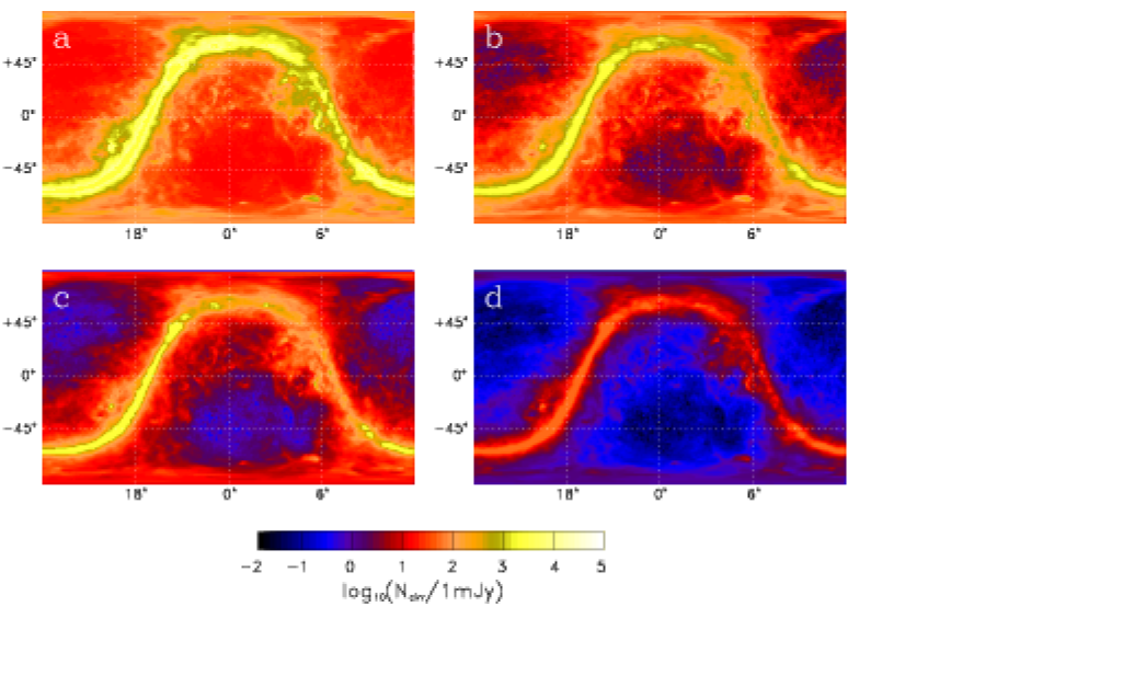
Figure 6: Comparison of predicted cirrus confusion noise levels of four different FIR instruments at their resolution limits. Confusion noise levels are displayed over the range as given by the colour-bar. All maps were constructed with no DIRBE–ISOPHOT conversion applied and with constant $\alpha$ and are presented in an equatorial coordinate system (J2000). (a) ISO/ISOPHOT C200 camera, 170 $\mu$m; (b) ASTRO-F/FIS 170 $\mu$m; (c) Spitzer/MIPS 160 $\mu$m; (d) Herschel/PACS 175 $\mu$m. For a surface brightness of B $>$ 200 MJy sr^-1 the cirrus confusion noise values given in this figure are lower limits and represent the confusion noise value at B $=$ 200 MJy sr^-1.

6 Summary

In this paper we present the results of a detailed investigation of the dependence of the sky confusion noise and in particular the cirrus confusion noise on measurement configurations for the long-wavelength ($\lambda$ $\geq$ 90 $\mu$m) observations with ISOPHOT. Tables 2–7 together with Eq. 4 provide an easy tool to estimate confusion noise values. Based on these results and transformations for non-investigated filters we constructed all-sky confusion noise maps (stored as FITS files at: http://kisag.konkoly.hu/ISO/toolbox.html) for all possible measurement configurations of the P3 100 $\mu$m, C100 90, 100 and 105 $\mu$m and C200 120, 150, 170, 180 and 200 $\mu$m filters. These files can efficiently be used to estimate the confusion noise at any specific sky position even if the background surface brightness cannot be properly estimated from the measurement itself. From Version 7 onward the ISO Data Archive provides confusion noise values for individual ISOPHOT measurements, based on our numbers.

The results of the ISOPHOT confusion noise analysis and the utilization of simulated fractal maps allowed us to calculate cirrus confusion noise value ratios of ISOPHOT and other far-infrared spaceborn instruments. Using these values, all-sky maps with cirrus confusion noise estimates for point sources were constructed. This was done for the resolution limits of detectors of Spitzer/MIPS, ASTRO-F/FIS and Herschel/PACS. These maps can be used for the preparation of FIR observations with future space telescopes indicating sensitivity limits due to cirrus confusion noise. However, for passively cooled large telescopes (like HERSCHEL) other noise components like the thermal telescope background (see e.g. Okumura, 2001) or the extragalactic background will play a more dominant role.