Bounds on CDM and neutrino isocurvature perturbations from CMB and LSS data

Abstract

Generic models for the origin of structure predict a spectrum of initial fluctuations with a mixture of adiabatic and isocurvature perturbations. Using the observed anisotropies of the cosmic microwave backgound, the matter power spectra from large scale structure surveys and the luminosity distance vs redshift relation from supernovae of type Ia, we obtain strong bounds on the possible cold dark matter/baryon as well as neutrino isocurvature contributions to the primordial fluctations in the Universe. Neglecting the possible effects of spatial curvature and tensor perturbations, we perform a Bayesian likelihood analysis with thirteen free parameters, including independent spectral indexes for each of the modes and for their cross-correlation angle. We find that around a pivot wavenumber of $k=0.05\,h\,$Mpc^-1 the amplitude of the correlated isocurvature component cannot be larger than about 60% for the cold dark matter mode, 40% for the neutrino density mode, and 30% for the neutrino velocity mode, at 2 sigma. In the first case, our bound is larger than the WMAP first-year result, presumably because we prefer not to include any data from Lyman-$\alpha$ forests, but then obtain large blue spectral indexes for the non-adiabatic contributions. We also translate our bounds in terms of constraints on double inflation models with two uncoupled massive fields.

I Introduction

With the increasing precision of the measurements of the cosmic microwave background (CMB) anisotropies and large scale structures (LSS) of the universe as well as various other astronomical observations, it is now possible to have a clear and consistent picture of the history and content of the universe since nucleosynthesis. Although the now widely used term of “Standard Model of Cosmology” might remain premature as our knowledge of the cosmological scenario is by far less precise than that of the Standard Model of particle physics, the matter content of the universe as well as its expansion rate are now known within a precision of a few percents with great confidence. It is also well established that the cosmological perturbations which gave rise to the CMB anisotropies and the LSS of the universe was inflationary like, with a close to scale invariant Harrison-Zeldovitch spectrum. Moreover, the measurement of both the temperature and polarization anisotropies of the cosmic microwave background allows to test the paradigm of adiabaticity of the cosmological perturbations and hence the precise nature of the mechanism whih has generated them.

The simplest realizations of the inflationary paradigm predict an approximately scale invariant spectrum of adiabatic and Gaussian curvature fluctuations, whose amplitude remains constant outside the horizon, and therefore allows cosmologists to probe the physics of inflation through observations of the CMB anisotropies and the LSS matter distribution. However, this is certainly not the only possibility. Models of inflation with more than one field generically predict that, together with this so-called adiabatic component, there should also be entropy, or isocurvature perturbations Linde:1985yf ; Polarski:1994rz ; Garcia-Bellido:1995qq ; Gordon:2000hv ; Wands:2002bn ; Finelli:2000ya , associated with fluctuations in number density between different components of the plasma before photon decoupling, with a possible statistical correlation between the adiabatic and isocurvature modes Langlois:1999dw . Baryon and cold dark matter (CDM) isocurvature perturbations were proposed long ago Efstathiou:1986 as an alternative to adiabatic perturbations. A few years ago, two other modes, neutrino isocurvature density and velocity perturbations, have been added to the list Bucher:1999re . Moreover, it is well known that entropy perturbations seed curvature perturbations outside the horizon Polarski:1994rz ; Garcia-Bellido:1995qq ; Gordon:2000hv , so that it is possible that a significant component of the observed adiabatic mode could be strongly correlated with an isocurvature mode. Such models are generically called curvaton models Lyth:2001nq ; Moroi:2001ct , and are now widely studied as an alternative to the standard paradigm. Furthermore, isocurvature modes typically induce non-Gaussian signatures in the spectrum of primordial perturbations.

In this paper, we describe in more detail the analysis performed in Ref Crotty:2003aa , constraining the various isocurvature components. We also extend it by including additional observational constraints, and extra free parameters in the model. We use data from the temperature power spectrum and temperature-polarization cross-correlation measured by the WMAP satellite WMAP ; as well as from the small-scale temperature anisotropy probed by VSA VSA , CBI CBI and ACBAR ACBAR ; from the matter power spectrum measured by the 2-degree-Field Galaxy Redshift Survey (2dFGRS) 2dFGRS and the Sloan Digital Sky Survey (SDSS) SDSS ; and also use data from the recent type Ia Supernova compilation of Ref. Riess2004 . We do not use the data from Lyman-$\alpha$ forests, since they are based on non-linear simulations carried under the assumption of adiabaticity. The first bounds on isocurvature perturbations assumed uncorrelated modes Stompor:1995py , but recently also correlated ones were considered in Refs. Trotta:2001yw ; Amendola:2001ni ; Gordon:2002gv ; Valiviita:2003ty ; Crotty:2003aa ; Bucher:1999re ; Moodley:2004ws . Our general analysis includes this possibility. In the first part of this work, we will not assume any specific model of inflation, nor any particular mechanism to generate the perturbations (late decays, phase transitions, cosmic defects, etc.), and thus will allow all five modes — adiabatic (AD), baryon isocurvature (BI), CDM isocurvature (CDI), neutrino isocurvature density (NID) and neutrino isocurvature velocity (NIV) — to be correlated (or not) with each other , and to have arbitrary tilts.

In terms of model building, the simplest situation beyond the paradigm of adiabaticity is that of a single isocurvature mode mixed with the adiabatic one. Therefore, we shall not consider more than one isocurvature mode at a time, and our primordial perturbations will be described by three amplitudes and three spectral indices, associated respectively with the adiabatic, isocurvature and cross-correlated components. This choice is somewhat different from that of Refs. Trotta:2001yw ; Bucher:1999re ; Moodley:2004ws , who introduce several modes at a time, but a single tilt for each power spectrum of primordial perturbations. The assumption that all the modes have comparable amplitudes and a common tilt are both difficult to motivate theoretically and, to our knowledge, all proposed mechanisms based on inflation stand far from this case. For instance, double inflation leads to at most one isocurvature mode, always with a tilt differing from the adiabatic one; on the other hand, the curvaton scenario predicts a single tilt, but only one isocurvature mode, fully correlated or anti-correlated with the adiabatic mode. However, in the absence of any theoretical prior, we believe the approach of Refs. Trotta:2001yw ; Bucher:1999re ; Moodley:2004ws is interesting and complementary to ours.

For simplicity, we will neglect the possible effects of spatial curvature and tensor perturbations, and assume that neutrinos are massless Pastor . Each model will be described by eleven cosmological parameters: the six usual parameters of the standard $\Lambda$CDM model; the amplitude and spectral index of the primordial isocurvature perturbation; the amplitude and spectral index of the cross-correlation angle between the adiabatic and isocurvature modes; and finally, a parameter $w$ describing the equation of state of dark energy, assumed to be time-independent as a first approximation. In addition, we will treat conservatively the matter-to-light bias of the 2dF and SDSS redshift surveys as two extra free parameters.

In section II we describe the notation we use in our analysis of isocurvature modes and discuss the relation with multi-field inflation, and in particular two-field models, on which we will concentrate ourselves. In section III we discuss the general bounds on our full parameter space from CMB, LSS and SN data using a Bayesian likelihood analysis. In section IV we analyze those bounds in a concrete model of two-field inflation: double inflation, with two uncoupled massive fields. A particular case is that in which the two fields have equal masses, like in complex field inflation, which we show is not ruled out. In section V we present our general conclusions.

II Notations

For the theoretical analysis, we will use the notation and some of the approximations of Refs. Gordon:2000hv ; Wands:2002bn . During inflation more than one scalar field could evolve sufficiently slowly that their quantum fluctuations perturb the metric on scales larger than the Hubble scale during inflation. These perturbations will later give rise to one adiabatic mode and several isocurvature modes. We will restrict ourselves here to the situation where there are only two fields, $\phi_{1}$ and $\phi_{2}$, and thus only one isocurvature and one adiabatic mode. Introducing more fields would complicate the inflationary model and even then, it would be rather unlikely that more than one isocurvature mode contributes to the observed cosmological perturbations.

The evolution during inflation will draw a trajectory in field space. Perturbations along the trajectory (i.e. in the number of $e$-folds $N$) will give rise to curvature perturbations on comoving hypersurfaces,

$${\cal R}_{k}=\delta N_{k}=H\,\delta t_{k}=H\,{\delta\rho_{k}\over\dot{\rho}}\,,$$ (1)

while perturbations orthogonal to the trajectory will give rise to gauge invariant entropy (isocurvature) perturbations,

$${\cal S}=\delta\ln{n_{i}\over n_{j}}={\delta\rho_{i}\over(\rho_{i}+p_{i})}-{\delta\rho_{j}\over(\rho_{j}+p_{j})}\,.$$ (2)

For instance, entropy perturbations in cold dark matter during the radiation era can be computed as ${\cal S}_{\rm CDI}=\delta_{\rm cdm}-3\delta_{\gamma}/4$. In order to relate these perturbations during the radiation era with those produced during inflation, one has to follow the evolution across reheating.

During inflation we can always perform an instantaneous rotation along the field trajectory and relate the gauge-independent perturbations in the fields Bardeen , $\delta\hat{\phi}_{i}=\delta\phi_{i}+(\dot{\phi}_{i}/H)\psi$, with perturbations along and orthogonal to the trajectory, $\delta\sigma$ and $\delta s$,

$$\left(\begin{array}[]{c}\delta\sigma\\[5.69054pt] \delta s\end{array}\right)=\left(\begin{array}[]{rr}\cos\varphi&\sin\varphi\\[5.69054pt] -\sin\varphi&\cos\varphi\end{array}\right)\left(\begin{array}[]{c}\delta\hat{\phi}_{1}\\[5.69054pt] \delta\hat{\phi}_{2}\end{array}\right)\,,$$ (3)

with $\varphi$ the rotation angle between the two frames.

In this case, the curvature and entropy perturbations on super-horizon scales can be written, in the slow-roll approximation, as Garcia-Bellido:1995qq ; Gordon:2000hv

$${\cal R}_{k}=H\,{\dot{\phi}_{1}\delta\hat{\phi}_{1}+\dot{\phi}_{2}\delta\hat{\phi}_{2}\over\dot{\phi}_{1}^{2}+\dot{\phi}_{2}^{2}}=H\,{\delta\sigma_{k}\over\dot{\sigma}}\,,$$ (4)

$$\,{\cal S}_{k}=\frac{2}{3}\dot{\varphi}\,{\dot{\phi}_{1}\delta\hat{\phi}_{2}-\dot{\phi}_{2}\delta\hat{\phi}_{1}\over\dot{\phi}_{1}^{2}+\dot{\phi}_{2}^{2}}=\frac{2}{3}\dot{\varphi}\,{\delta s_{k}\over\dot{\sigma}}\,.$$ (5)

where $\dot{\sigma}^{2}\equiv\dot{\phi}_{1}^{2}+\dot{\phi}_{2}^{2}$. The problem however is that, contrary to the case of purely adiabatic perturbations, the amplitudes of both curvature and entropy perturbations do not remain constant on superhorizon scales, but evolve with time Polarski:1994rz ; Garcia-Bellido:1995qq . In particular, due to the conservation of the energy momentum tensor, the entropy perturbations seed the curvature perturbations, and thus their amplitude during the radiation dominated era evolves according to Garcia-Bellido:1995qq ; Gordon:2000hv

$$\dot{\cal R}_{k}=\alpha(t)H\,{\cal S}_{k}\,,$$ (6)

$$\,\dot{\cal S}_{k}=\beta(t)H\,{\cal S}_{k}\,,$$ (7)

where $\alpha$ and $\beta$ are time-dependent functions characterizing the evolution during inflation and radiation eras. A formal solution can be found in terms of a transfer matrix, relating the amplitude at horizon crossing during inflation (*) with that at a later time during radiation,

$$\left(\begin{array}[]{c}{\cal R}\\[5.69054pt] {\cal S}\end{array}\right)=\left(\begin{array}[]{lr}1&T_{{\cal R}{\cal S}}\\[5.69054pt] 0&T_{{\cal S}{\cal S}}\end{array}\right)\left(\begin{array}[]{c}{\cal R}_{*}\\[5.69054pt] {\cal S}_{*}\end{array}\right)\,,$$ (8)

where the transfer functions are given by Gordon:2000hv

$$T_{{\cal S}{\cal S}}(t,t_{*})=\exp\left[\int_{t_{*}}^{t}\beta(t^{\prime})H(t^{\prime})dt^{\prime}\right]\,,$$ (9)

$$T_{{\cal R}{\cal S}}(t,t_{*})=\int_{t_{*}}^{t}\alpha(t^{\prime})H(t^{\prime})T_{{\cal S}{\cal S}}(t^{\prime},t_{*})dt^{\prime}\,.$$ (10)

Note that in the absence of primordial isocurvature perturbation, ${\cal S}_{*}=0$, the curvature perturbation remains constant and no isocurvature perturbation is generated during the evolution. This is the reason for the entries $T_{{\cal R}{\cal R}}=1$ and $T_{{\cal S}{\cal R}}=0$, respectively, in the transfer matrix. Note also that in many models, $\alpha(t)$ and $\beta(t)$ vanish after reheating, so that $({\cal R}_{k},{\cal S}_{k})$ remain constant during radiation domination on super-horizon scales. However, this is not true for instance when the fluid carrying the isocurvature perturbations has a significant background density (compared to the total Universe density), as assumed in the curvaton scenario.

Since $\phi_{1}$ and $\phi_{2}$ are essentially massless during inflation, we can treat them as free fields whose fluctuations at horizon crossing have an amplitude $\delta\hat{\phi}_{i}=(H_{k}/\sqrt{2k^{3}})\,e_{i}({\bf k})$, where $H_{k}$ is the rate of expansion at the time the perturbation crossed the horizon $(k_{*}=aH)$, and $e_{i}({\bf k})$ are Gaussian random fields with zero mean, $\langle e_{i}({\bf k})\rangle=0$ and $\langle e_{i}({\bf k})e_{j}^{*}({\bf k}^{\prime})\rangle=\delta_{ij}\,\delta({\bf k}-{\bf k}^{\prime})$. Now, since $\delta\sigma_{k}$ and $\delta s_{k}$ and just rotations of the field fluctuations, they are also Gaussian random fields of amplitude $H_{k}/\sqrt{2k^{3}}$. However, the time evolution (6) will mix those modes and will generically induce correlations and non Gaussianities.

Therefore, the two-point correlation function or power spectra of both adiabatic and isocurvature perturbations, as well as their cross-correlation, can be parametrized with three power laws, i.e. three amplitudes and three spectral indices,

$$\Delta_{\cal R}^{2}(k)\! \equiv \!{k^{3}\over 2\pi^{2}}\langle{\cal R}^{2}\rangle=A^{2}\,\left({k\over k_{0}}\right)^{n_{\rm ad}-1}\,,$$

$$\Delta_{\cal S}^{2}(k)\! \equiv \!{k^{3}\over 2\pi^{2}}\langle{\cal S}^{2}\rangle=B^{2}\,\left({k\over k_{0}}\right)^{n_{\rm iso}-1}\,,$$ (11)

$$\Delta_{{\cal R}{\cal S}}^{2}(k)\! \equiv \!{k^{3}\over 2\pi^{2}}\langle{\cal R}{\cal S}\rangle\,$$

$$= A\,B\,\cos\Delta_{k_{0}}\left({k\over k_{0}}\right)^{n_{\rm cor}+{1\over 2}(n_{\rm ad}+n_{\rm iso})-1}\,,$$

where $k_{0}$ is some pivot scale. Since the time of horizon crossing $t_{*}$ in the transfer functions (9) is scale-dependent, the correlation angle $\Delta(k)$ is in general a function of $k$. In the above definitions, we approximated $\cos\Delta(k)$ by a power law with amplitude $\cos\Delta_{k_{0}}$ and tilt $n_{\rm cor}$. So, we assumed implicitly that the inequality

$$\left|\cos\Delta_{k_{0}}\right|\left({k\over k_{0}}\right)^{n_{\rm cor}}\leq 1$$ (12)

holds over all relevant scales. In the following analysis, we will impose that for each value of $\cos\Delta_{k_{0}}$ the tilt $n_{\rm cor}$ is restricted to the interval in which the inequality holds between $k_{\rm min}=4\times 10^{-5}$Mpc^-1 and $k_{\rm max}=0.5\,$Mpc^-1, which is roughly the range probed by our CMB and LSS data sets. Far from that range, we expect that next-order terms become important and that the power-law approximation breaks down. The fact that $n_{\rm cor}$ can be non-zero was already considered in a recent paper Valiviita:2003ty .

The angular power spectrum of temperature and polarization anisotropies seen in the CMB today can be obtained from the radiation transfer functions for adiabatic and isocurvature perturbations, $\Theta_{l}^{\rm ad}(k)$ and $\Theta_{l}^{\rm iso}(k)$, computed from the initial conditions $({\cal R}_{\rm rad},{\cal S}_{\rm rad})=(1,0)$ and $(0,1)$, respectively, and convolved with the initial power spectra,

$$C_{l}^{\rm ad}\! \equiv \,\int{dk\over k}\,\left[\Theta_{l}^{\rm ad}(k)\right]^{2}\,\left({k\over k_{0}}\right)^{n_{\rm ad}-1}\,,$$

$$C_{l}^{\rm iso}\! \equiv \,\int{dk\over k}\,\left[\Theta_{l}^{\rm iso}(k)\right]^{2}\,\left({k\over k_{0}}\right)^{n_{\rm iso}-1}\,,$$

$$C_{l}^{\rm cor}\! \equiv \,\int{dk\over k}\,\Theta_{l}^{\rm ad}(k)\,\Theta_{l}^{\rm iso}(k)\,\left({k\over k_{0}}\right)^{n_{\rm cor}+{1\over 2}(n_{\rm ad}+n_{\rm iso})-1}\,,$$

Then, the total angular power spectrum reads

$$C_{l}=A^{2}\,C_{l}^{\rm ad}+B^{2}\,C_{l}^{\rm iso}+2\,A\,B\,\cos\Delta_{k_{0}}\,C_{l}^{\rm cor}\,.$$ (13)

In many works (see for instance Amendola:2001ni ; WMAP ), the following parametrization is employed:

$$C_{l}=C_{l}^{\rm ad}+{\cal B}^{2}\,C_{l}^{\rm iso}+2{\cal B}\,\cos\Delta_{k_{0}}\,C_{l}^{\rm cor}\,,$$ (14)

where the global normalization has been marginalized over, and ${\cal B}$ is the entropy to curvature perturbation ratio during the radiation era, ${\cal B}\equiv{\cal S}_{\rm rad}/{\cal R}_{\rm rad}$. We will use here a slightly different notation, used before by other groups Langlois:1999dw ; Stompor:1995py , where $A^{2}\equiv(1-\alpha)$ and $B^{2}\equiv\alpha$ (up to a global normalization factor), so that

$$C_{l}=(1-\alpha)\,C_{l}^{\rm ad}+\alpha\,C_{l}^{\rm iso}+2\beta\,\sqrt{\alpha(1-\alpha)}\,C_{l}^{\rm cor}\,.$$ (15)

The parameter $\alpha$ runs from purely adiabatic ($\alpha=0$) to purely isocurvature ($\alpha=1$), while $\beta$ defines the correlation coefficient, with $\beta=+1(-1)$ corresponding to maximally correlated(anticorrelated) modes. There is an obvious relation between both parametrizations:

$$\alpha={\cal B}^{2}/(1+{\cal B}^{2})\,,\hskip 28.45274pt\beta=\cos\Delta_{k_{0}}\,.$$ (16)

This notation has the advantage that the full parameter space of $(\alpha,\ 2\beta\sqrt{\alpha(1-\alpha)})$ is contained within a circle of radius $1/2$. The North and South rims correspond to fully correlated ($\beta=+1$) and fully anticorrelated ($\beta=-1$) perturbations, with the equator corresponding to uncorrelated perturbations ($\beta=0$). The East and West correspond to purely isocurvature and purely adiabatic perturbations, respectively. Any other point within the circle is an arbitrary admixture of adiabatic and isocurvature modes.

Note that interpreting the results in non fully correlated and anti correlated models is made difficult by the fact that as soon as $n_{\rm cor}\neq 0$, the contours one obtains depend on the choice of the pivot scale. For example in the simple case where $n_{\rm ad}=n_{\rm iso}$, the relative amplitude between $C_{l}^{\rm ad}$ and $C_{l}^{\rm iso}$ is unchanged when one changes the pivot scale, and hence $\alpha$ is unchanged, but the correlation angle $\Delta(k)$, and hence $\beta$ changes with the pivot scale as $\beta(k_{1})=\beta(k_{0})(k_{1}/k_{0})^{n_{\rm cor}}$. In our example, if $n_{\rm cor}>0$, points within the $(\alpha,\ 2\beta\sqrt{\alpha(1-\alpha)})$ circle are shifted vertically toward the edge of the circle when one increases the pivot scale and shifted toward the horizontal $\beta=0$ line when one decreases the pivot scale.

We should emphasize that the three amplitude parameters $\ln[10^{10}{\cal R}_{\rm rad}]$, $\alpha$ and $\beta$ are defined at $k=k_{0}$, and that comparing bounds from various papers is straighforward only when the pivot scale is the same. Throughout this paper, we will use $k_{0}=0.05$ Mpc^-1, which differs from our previous work Crotty:2003aa , but has the advantage of matching most of the literature. This value of $k$ corresponds roughly to multipole number $l_{0}\sim 300$.

III General results

We computed the Bayesian likelihood of each cosmological parameter with a Monte Carlo Markov Chain method, using the public code CosmoMC cosmomc with option MPI in the COSMOS supercomputer. For each case, we ran 32 Markhov chains, and obtained between 30,000 and 60,000 samples (without including the multiplicity of each point).

We used the public code CAMB camb in order to compute the theoretical prediction for the $C_{l}$ coefficients of the temperature and polarization power spectra, as well as the matter spectra $P(k)$, for all four different components (The BI mode is just a rescaling of the CDI mode, see below). Moreover, we slightly modified the interface between CAMB and CosmoMC in order to include the cross-correlated power spectra, as well as three independent tilts $-$ in the CosmoMC jargon, the three tilts and the three amplitudes were implemented into the code as “fast parameters”, in order to save a considerable amount of time. The likelihood of each model was then computed using the detailed information provided on the experimental websites (or directly from the corresponding routines of the CosmoMC code when available), using three groups of data sets: i) CMB data: 1398 points from WMAP ($2\leq l\leq 900$) WMAPlike , 8 points from VSA ($580\leq l\leq 1700$) VSA , 8 points from CBI ($700\leq l\leq 1800$) CBI , 7 points from ACBAR ($920\leq l\leq 1960$) ACBAR ; ii) LSS data: 32 points from 2dFGRS (up to $k_{\rm max}=0.1\ h$ Mpc^-1) 2dFGRS , 17 points from SDSS (up to $k_{\rm max}=0.15\ h$ Mpc^-1) SDSS ; and iii) SNIa data: 157 points from Riess et al. Riess2004 . We have checked that the inclusion of the HST Freedman:2000cf and BBN priors are irrelevant for the determination of the Hubble parameter and the baryon density; that is, the data from CMB, LSS and SNIa is enough in order to determine these parameters, and therefore we ignored the priors in the final analysis.

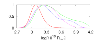
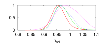
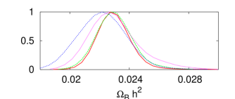
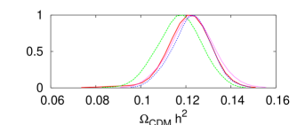
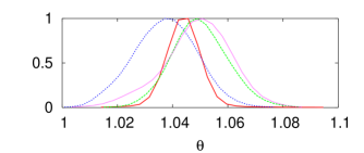
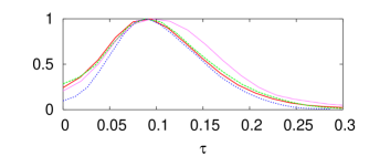
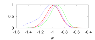
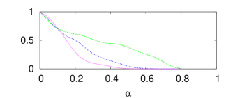
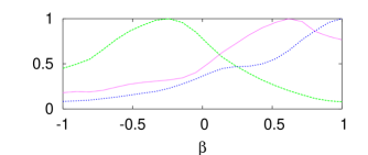
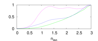
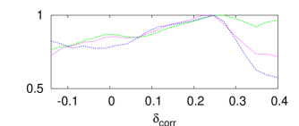
Figure 1: The one-dimensional likelihood functions for our basis of eleven independent cosmological parameters (not including the tilts of the two redshift surveys), for the adiabatic mode alone (AD) or mixed with the three different types of isocurvature modes (AD+CDI, AD+NID, AD+NIV). The first seven parameters are those of the standard $\Lambda$CDM model, extended to dark energy with a constant equation of state. The last four parameters $(\alpha,\beta,n_{\rm iso},\delta_{\rm cor})$ describe the isocurvature initial conditions. ($\delta_{\rm cor}$ is define in Eq. (17.))

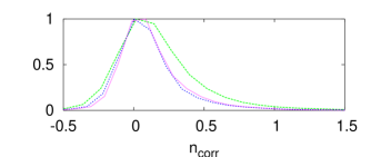
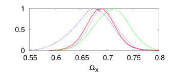
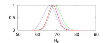
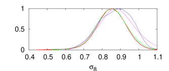
Figure 2: Continuation of figure 1, showing the 1D likelihood of some derived cosmological parameters, for the same cases. These likelihoods should be considered with care, because the parameters shown here do not belong to the basis used by the Markov chain algorithm. Therefore, the shape of the above likelihoods depends not only on the likelihood of the underlying parameters, but also on the properties of the functions relating them to the parameters of the basis. This explains for instance why $n_{\rm cor}=\delta_{\rm cor}\,\ln(|\beta|^{-1})$ seems to be well-constrained, while $\delta_{\rm cor}$ and $\beta$ are not.

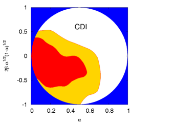
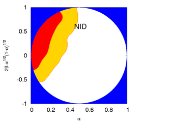
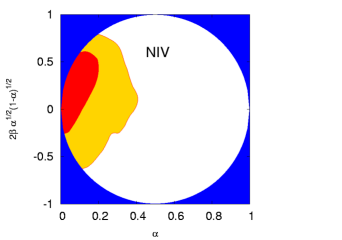
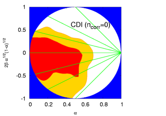
Figure 3: The 2-$\sigma$ contours of $\alpha$ and the cross-correlated mode coefficient $2\beta\sqrt{\alpha(1-\alpha)}$, for a) the CDI isocurvature mode; b) the NID mode; c) the NIV mode; d) the CDI mode, with the constraint $n_{\rm cor}=0$ and the contours of equal $2(R^{2}-1)/s_{k}=0,\pm 0.5,\pm 1,\pm 2$ from double inflation.

In order to take into account the $\beta$-dependent constraint on $n_{\rm cor}$, see eq. (12), we choose to define a new parameter

$$\delta_{\rm cor}\equiv n_{\rm cor}/\ln(|\beta|^{-1}),$$ (17)

whose boundaries are fixed once and for all by the values of the pivot scale and the scales ($k_{\rm min}$, $k_{\rm max}$) introduced in the previous section. The basis of cosmological parameters used by the Markov Chain algorithms consists on: (i) the seven parameters describing the standard adiabatic $\Lambda$CDM model, extended to dark energy with a constant equation of state, and (ii) the four parameters describing the admixture of one (correlated) isocurvature mode, already defined in the previous section. More explicitely, we use the following basis: 1) the overall normalisation parameter $\ln[10^{10}{\cal R}_{\rm rad}]$ where ${\cal R}_{\rm rad}$ is the curvature perturbation in the radiation era; 2) the adiabatic tilt $n_{\rm ad}$; 3) the baryon density $\omega_{\rm B}=\Omega_{\rm B}h^{2}$; 4) the cold dark matter density $\omega_{\rm cdm}=\Omega_{\rm cdm}h^{2}$; 5) the ratio $\theta$ of the sound horizon to the angular diameter distance multiplied by 100; 6) the optical depth to reionization $\tau$; 7) the dark energy equation of state parameter $w$; then, for the isocurvature sector; 8) the isocurvature contribution $\alpha$; 9) the cross-correlation parameter $\beta$; 10) the isocurvature tilt $n_{\rm iso}$; 11) the parameter $\delta_{\rm cor}$ which determines the cross-correlation tilt $n_{\rm cor}$; and finally, two arbitrary bias parameters associated to the 2dF and SDSS power spectrum. Our full parameter space is therefore 13-dimensional.

We did not devote a specific analysis to the case of the baryon isocurvature modes, which is qualitatively similar to that of CDI modes, since the spectra are simply rescaled by a factor $\Omega_{\rm B}^{2}/\Omega_{\rm cdm}^{2}$ ($\Omega_{\rm B}/\Omega_{\rm cdm}$ for the cross-correlation): thus, compared to the AD + CDI case, significantly larger values of $\alpha$ will be allowed in the AD + BI case. Like in other recent analyses, we find that the inclusion of isocurvature modes does not improve significantly the goodness-of-fit of the cosmological model, since in the AD+CDI, AD+NID and AD+NIV cases the minimum $\chi^{2}$ is always between 1672 and 1674 for 1614 degrees of freedom, to be compared with 1674 for 1618 degrees of freedom in the pure adiabatic case. Therefore, the question is just to study how much departure from the standard picture is allowed, by computing the Bayesian confidence limit on the isocurvature parameters. A more detailed analysis of model comparison with Bayesian Information Criteria Liddle:2004nh will be done in a follow up paper.

On Fig. 1 we plot the marginalised likelihood for our basis of eleven cosmological parameters, in the cases AD+CDI, AD+NID and AD+NIV, compared with the pure adiabatic case. Figure 2 shows the likelihood of some derived parameters. It appears that most parameters are robust against the inclusion of isocurvature perturbations (this is in agreement with the conclusion of Ref. Moodley:2004ws that with only one isocurvature mode present, no significant parameter degeneracy pops out). Our 95% C.L. on $\alpha$ in the three cases is given in Table 1.

Table 1: The one-dimensional 2-$\sigma$ ranges on the isocurvature mode coefficients for the various models.

model	$\alpha$	$2\beta\,[\alpha(1-\alpha)]^{1/2}$
AD+CDI	$<0.6$	$-0.7$  to  $0.3$
AD+NID	$<0.4$	$-0.2$  to  $0.8$
AD+NIV	$<0.3$	$-0.4$  to  $0.6$

Note that in the limit $\alpha=0$, the three parameters $\beta$, $n_{\rm iso}$, $\delta_{\rm cor}$ become irrelevant. So, the fact that pure adiabatic models are very good fits implies that these parameters are loosely constrained. This explains why the corresponding likelihoods on Fig. 1 are not well-peaked like for other parameters. In addition, these likelihoods should be considered with great care, because it is difficult for the Markhov Chains to explore in detail the tails of the multi-dimensionnal likelihood corresponding to tiny values of $\alpha$, where basically any value of ($\beta$, $n_{\rm iso}$, $\delta_{\rm cor}$) are allowed. Therefore, increasing the number of samples would tend to flatten these likelihoods, while the other ones would remain stable (as we checked explicitely). However, it is clear that all models prefer a large isocurvature tilt and saturate the bound $n_{\rm iso}<3$ that we fixed in the present analysis. This feature is important for understanding our results and comparing with other analyses, as explained in the last paragraph of this section.

On Fig. 3, we plot the two-dimensional confidence levels directly for the isocurvature and cross-correlation coefficients ($\alpha$, $2\beta\sqrt{\alpha(1-\alpha)}$) in the three cases AD+CDI, AD+NID and AD+NIV. The last plot corresponds to the AD+CDI case with a prior $n_{\rm cor}=0$ which is relevant for the bounds on double inflation, but the results are not substantially different from the general AD+CDI case. We see that the AD+CDI model slightly prefers anti-correlated cases (note that $\beta<0$ means a positive contribution from the cross-correlated component), while AD+NID and AD+NIV models clearly prefer correlated ones.

On Figure 4, we plot the CMB and LSS power spectra for two particular CDI and NID models. In order to get a better understanding of our bounds, we chose models with large values of $\alpha$, still allowed at the 2-$\sigma$ level: respectively, $\alpha=0.53$ and $\alpha=0.41$. The detailed values of other cosmological parameters for these models are given in the figure caption. In the CDI example, one can see that the non-adiabatic contributions to all spectra remain tiny, excepted for the matter power spectrum on scales $k>0.2h\,$Mpc^-1, due to the large isocurvature tilt $n_{\rm iso}=2.93$ of the model. This is an indication that our $\alpha$ bound in the CDI case depends very much on constraints on the small-scale matter power spectrum, while future improvements in the determination of CMB spectra would not reduce it dramatically. Note that a precise experimental determination of the amplitude parameter $\sigma_{8}$ (which is mainly sensitive to scales around $k=0.2\,h$ Mpc^-1) would probably not change things either, since our CDI models have roughly the same $\sigma_{8}$ values as purely adiabatic well-fitting models (see Figure 2); on the other hand, any constraint on smaller wavelengths could improve the bounds. This means in particular that our choice not to include the Lyman-$\alpha$ data plays a crucial role in our results.

The same conclusions apply to the NID model of Fig. 4. In addition, in the NID case, we see that the non-adiabatic contribution is significant also for small-scale ($l>200$) temperature and polarization spectra. Indeed, it is well-known that the NID isocurvature and cross-correlated modes can mimick the adiabatic CMB spectra to a better extent than CDI modes (essentially because the amplitude of the secondary peaks is not strongly supressed). So, in the NID case, future improvement in the CMB data should help to improve the bounds on the isocurvature fraction.

Our bounds are difficult to compare with those of Ref. Moodley:2004ws , because of our different parameter space, observational data set and conventions of normalization. In the AD+CDI case, our analysis is closer to the one of the WMAP team WMAP , although we have more free cosmological parameters ($n_{\rm cor}$, $w$), more data (SDSS, CBI, VSA) and less constraints on the matter–to–light bias. The 95% limit ${\cal B}<0.33$ obtained by WMAP would correspond to $\alpha<0.1$ in our notations, which is significantly smaller than our results. Also, The WMAP $1\sigma$ bounds on $n_{\rm iso}$ are $1.26\pm 0.5$, while we find that the likelihood peaks at our maximum allowed value $n_{\rm iso}=3$. The most likely explanation is that the use of the Lyman-$\alpha$ data in the WMAP analysis eliminates all our well-fitting models with $n_{\rm iso}>2$ and large $\alpha$ values. Similar conclusions apply to our previous results Crotty:2003aa , in which we did not use any Lyman-$\alpha$ information, but adopted a flat prior $0.6<n_{\rm iso}<1.5$ (this was the interval in which our grid of models was computed). Then, most of the well-fitting models of Crotty:2003aa had slighly negative values of $n_{\rm ad}-n_{\rm iso}$. Therefore, translating our previous results in terms of a pivot scale $k_{0}=0.05\,$Mpc^-1 would lead to a small decrease in the $\alpha$ bounds, making them comparable with the WMAP bound in the CDI case, and smaller than the conservative bounds of this work.

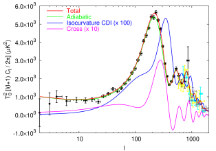
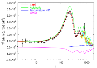
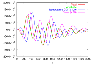
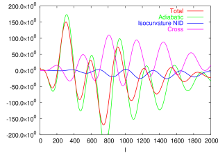
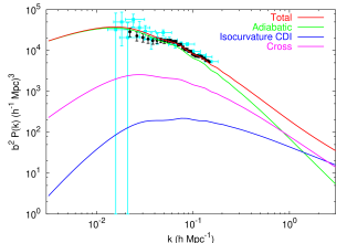
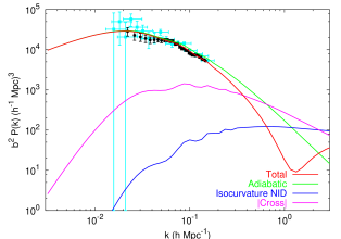
Figure 4: Temperature, E-polarization and matter power spectra for two particular CDI and NID models. In order to get a better understanding of our bounds, we chose here two models with large values of $\alpha$, still allowed at the 2-$\sigma$ level: respectively, $\alpha=0.53$ and $\alpha=0.41$. Other parameter values are for the CDI (resp. NID) model: $\omega_{\rm B}=0.0217$ (0.0196), $\omega_{\rm cdm}=0.112$ (0.131), $\theta=1.06$ (1.01), $\tau=0.068$ (0.131), $w=-0.88$ (-1.44), $n_{\rm ad}=0.96$ (1.02), $n_{\rm iso}=2.93$ (2.95), $n_{\rm cor}=0.05$ (0.03), $\ln[10^{10}{\cal R}_{\rm rad}]=3.73$ (3.98), $\beta=-0.62$ (0.88). The $\chi^{2}$ of the two models is respectively 1675 and 1674. From top to bottom, we show the $C_{l}^{\rm TT}$, $C_{l}^{\rm TE}$ and $P(k)$ power spectra, as well as the contribution of each component: adiabatic, isocurvature, cross-correlated, total. The CDI isocurvature and cross-correlated components have been rescaled by a factor indicated in each figure. We also show the data points that we use throughout the analysis, from WMAP (black), ACBAR (grey), CBI (blue), VSA (yellow), 2dF (black) and SDSS (blue). In the case of the matter power spectrum, one should not trust a “$\chi^{2}$-by-eye” comparison with the data: first, because the spectrum has to be convolved with the experimental window function before the comparison (this changes its slope significantly); second, because we show here the data points before rescaling by the two bias factors, which are left arbitrary for each experiment.

IV Double Inflation

In this section we will use the previous bounds to constrain the parameters of a concrete model of inflation called double inflation double ; Langlois:1999dw . This is an inflationary model with two massive fields, $\phi_{1}$ and $\phi_{2}$, of different masses, with ratio $R=m_{1}/m_{2}$. No coupling (except gravitational) between fields is assumed. The equations of motion and Friedmann equation can be written as

$$\ddot{\phi}_{1}+3H\,\dot{\phi}_{1}+m_{1}^{2}\phi_{1}=0\,,$$ (18)

$$\ddot{\phi}_{2}+3H\,\dot{\phi}_{2}+m_{2}^{2}\phi_{2}=0\,,$$ (19)

$$H^{2}={\kappa^{2}\over 6}\Big{(}\dot{\phi}_{1}^{2}+\dot{\phi}_{2}^{2}+m_{1}^{2}\phi_{1}^{2}+m_{2}^{2}\phi_{2}^{2}\Big{)}\,,$$ (20)

where $\kappa^{2}\equiv 8\pi G$. In the slow-roll approximation, $\dot{\phi}_{i}^{2}\ll m_{i}^{2}\phi_{i}^{2}\,;\ddot{\phi}_{i}\ll H\dot{\phi}_{i}$, we have the solutions double

$$\phi_{1}=\left({4s\over\kappa^{2}}\right)^{1/2}\,\sin\theta\,;\hskip 14.22636pt\phi_{2}=\left({4s\over\kappa^{2}}\right)^{1/2}\,\cos\theta\,,$$

with $s=-\ln(a/a_{\rm end})$ the number of $e$-folds to the end of inflation. For simplicity, we restrict ourselves to the case where $\phi_{1}$ and $\phi_{2}$ remain positive during inflation. Substituting into the rate of expansion,

$$H^{2}(s)\simeq{2\over 3}m_{2}^{2}\,s\,\Big{(}1+(R^{2}-1)\sin^{2}\theta\Big{)}\,,$$ (21)

and, using the equations of motion, one can integrate out

$${d\theta\over ds}(s)={\tan\theta\over 2s}\,{R^{2}-1\over 1+R^{2}\,\tan^{2}\theta}\,.$$ (22)

to obtain

$$s=s_{0}\,{(\sin\theta)^{2\over R^{2}-1}\over(\cos\theta)^{2R^{2}\over R^{2}-1}}\,.$$

As inflation proceeds, $s$ decreases and $\theta$ also decreases. We will call $s_{H}=60$ to the number of $e$-folds before the end of inflation when the scale corresponding to our Hubble radius today exited during inflation.

IV.1 Linear perturbations

The great advantage of double inflation is that it is possible to find explicit formulas for the perturbations on superhorizon scales. The growing mode solutions for the scalar fields and the scalar metric perturbation in the longitudinal gauge, and in the slow-roll approximation, are given by Polarski:1994rz

$$\Phi=-C_{1}(k){\dot{H}\over H^{2}}+C_{3}(k){2(R^{2}-1)R^{2}\phi_{1}^{2}\phi_{2}^{2}\over 3(R^{2}\phi_{1}^{2}+\phi_{2}^{2})^{2}}\,,\hskip 14.22636pt$$ (23)

$${\delta\phi_{1}\over\dot{\phi}_{1}}={C_{1}(k)\over H}+C_{3}(k){2H\phi_{2}^{2}\over R^{2}\phi_{1}^{2}+\phi_{2}^{2}}\,,$$ (24)

$${\delta\phi_{2}\over\dot{\phi}_{2}}={C_{1}(k)\over H}-C_{3}(k){2HR^{2}\phi_{1}^{2}\over R^{2}\phi_{1}^{2}+\phi_{2}^{2}}\,.$$ (25)

Since $\phi_{1}$ and $\phi_{2}$ are independent uncoupled scalar fields and essentially massless during inflation, we can use the general formalism of section II, and write, in the slow-roll approximation,

$$C_{1}(k)=-{\kappa^{2}\over 2}{H_{k}\over\sqrt{2k^{3}}}\Big{(}\phi_{1}\,e_{1}({\bf k})+\phi_{2}\,e_{2}({\bf k})\Big{)}\,,\hskip 14.22636pt$$ (26)

$$C_{3}(k)=-{3H_{k}\over 2\sqrt{2k^{3}}}\left({e_{1}({\bf k})\over m_{1}^{2}\phi_{1}}-{e_{2}({\bf k})\over m_{2}^{2}\phi_{2}}\right)\,,$$ (27)

where $H_{k}$ is the rate of expansion when the perturbation of wavenumber

$$k\simeq k_{H}\,e^{s_{H}-s_{k}}\,,$$ (28)

left the horizon during inflation, where the scale of our present horizon is $k_{H}^{-1}=3000\,h^{-1}$ Mpc.

We will now assume that the light scalar field decays at the end of inflation into the ordinary particles, giving rise to photons, neutrinos, electrons and baryons, while the cold dark matter (CDM) arises from the decay of the heavy field. In principle, part of the CDM could also be produced by the light field or the heavy field could also decay into ordinary particles, but we will ignore these possibilities here. Then, the perturbations in the comoving gauge take the form

$${\delta^{(c)}n_{\gamma}\over n_{\gamma}}={\delta^{(c)}n_{\nu}\over n_{\nu}}={\delta^{(c)}n_{B}\over n_{B}}\,,$$

and there is only one isocurvature mode, the CDI mode,

$${\cal S}\equiv\delta^{(c)}\ln{n_{\rm cdm}\over n_{\gamma}}=\delta^{(c)}_{\rm cdm}-{3\over 4}\delta^{(c)}_{\gamma}\,,$$

all of which are gauge invariant quantities. During the radiation era, the initial conditions of all these modes are described in terms of only two $k$-dependent quantites, $\Phi_{k}$ and $S_{k}$. The pure adiabatic initial conditions are given by the gravitational potential during the radiation era,

$$\Phi_{\rm rad}(k)={2\over 3}\,{\cal R}_{\rm rad}(k)={2\over 3}\,C_{1}(k)\,,$$

with $C_{1}(k)$ the amplitude of the growing adiabatic mode during inflation. On the other hand, the isocurvature initial conditions in the radiation era arise from the perturbations in the heavy field $\phi_{1}$ at the end of inflation. In the long wavelength limit, the perturbations of this field during reheating follow closely the field itself, so that its energy density perturbations satisfy, in the comoving gauge,

$${\delta\rho^{(c)}\over\rho}=2{\delta\phi_{1}\over\phi_{1}}=-{4\over 3}C_{3}(k)\,m_{1}^{2}$$

which is constant during inflation, across reheating and into the radiation era. The entropy perturbation is dominated by the CDM density perturbation during the radiation era, ${\cal S}_{\rm rad}\simeq\delta^{(c)}_{\rm cdm}$. Using the values of $C_{1}(k)$ and $C_{3}(k)$ during inflation, we can finally write

$${\cal R}_{\rm rad}(k)=-{\kappa H_{k}\over\sqrt{2k^{3}}}\sqrt{s_{k}}\Big{(}\sin\theta_{k}\,e_{1}({\bf k})+\cos\theta_{k}\,e_{2}({\bf k})\Big{)}\,,\hskip 14.22636pt$$ (29)

$${\cal S}_{\rm rad}(k)={\kappa H_{k}\over\sqrt{2k^{3}}}{1\over\sqrt{s_{k}}}\left({e_{1}({\bf k})\over\sin\theta_{k}}-{R^{2}\,e_{2}({\bf k})\over\cos\theta_{k}}\right)\,.$$ (30)

Note that the cross-correlation amplitude $\cos\Delta(k)$ is almost independent of $k$, due to the cancellation of the factor $s_{k}$ between ${\cal R}_{\rm rad}(k)$ and ${\cal S}_{\rm rad}(k)$, and to the fact that $\theta_{k}$ is a mild function of $k$, see Eq. (22). In this case, the tilt $n_{\rm cor}$ vanishes. The adiabatic and isocurvature tilts can be computed explicitly using (28)

$${\cal P}_{\cal R}(k)={k^{3}\over 2\pi^{2}}\langle|{\cal R}_{k}|^{2}\rangle\,,\hskip 14.22636pt{\cal P}_{\cal S}(k)={k^{3}\over 2\pi^{2}}\langle|{\cal S}_{k}|^{2}\rangle\,,\$$ (31)

$$n_{\rm ad}=1-{\partial\ln{\cal P}_{\cal R}(k)\over\partial\ln s}\,,\hskip 5.69054ptn_{\rm iso}=1-{\partial\ln{\cal P}_{\cal S}(k)\over\partial\ln s}\,,\hskip 14.22636pt$$ (32)

as functions of the angle $\theta$ and the mass ratio $R$,

$$n_{\rm ad}\! =\! 1-{2\over s}+{(R^{2}-1)\tan^{2}\theta\over 2s\,(1+R^{2}\tan^{2}\theta)^{2}}\,,$$ (33)

$$n_{\rm iso}\! =\! 1-{(R^{2}-1)(R^{6}\tan^{4}\theta-1)\over s(1+(R^{2}-1)\sin^{2}\theta)}\times$$ (35)

$$\hskip 28.45274pt{1\over(1+(R^{2}+R^{4})\tan^{2}\theta+R^{6}\tan^{4}\theta)}$$

¿From ${\cal P}_{\cal R}$ and ${\cal P}_{\cal S}$, we obtain the parameters

$$\alpha={R^{4}\tan^{2}\theta+1\over s_{k}^{2}\sin^{2}\theta+R^{4}\tan^{2}\theta+1}\,,\hskip 14.22636pt$$ (36)

$$\beta={(R^{2}-1)\sin\theta\over\sqrt{R^{4}\tan^{2}\theta+1}}\,.$$ (37)

We have plotted these parameters as a function of the angle $\theta$ in Fig. 5, for $s_{k}\simeq 60$.

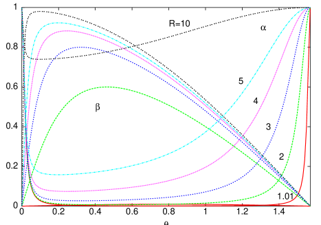
Figure 5: The values of parameters $\alpha$ and $\beta$ as a function of the angle $\theta$, for different values of the ratio $R=m_{1}/m_{2}$ in double inflation.

These parameters have maximum and minimum values given by

$$\alpha_{\rm min}={(R^{4}-1)^{3}\over(R^{4}-1)^{3}+s_{k}^{2}\Big{[}R^{8}-2R^{2}(R^{4}-1)-1\Big{]}}\,,\hskip 14.22636pt$$ (38)

$$\beta_{\rm max}={R^{2}-1\over R^{2}+1}\,,$$ (39)

as can be seen in Fig. 5.

IV.2 Bounds on double inflation

In this subsection we will impose the general bounds found in section III to the double inflation model double . Note that in this model it is assumed that the heavy field decays into cold dark matter, and therefore we only have one isocurvature component, CDI. The bounds from CDI will be used to constrain this particular model. We will leave for the future a detailed analysis of other two-field models of inflation.

In order to derive specific constraints, it will be useful to take into account the following relation between $\alpha$ and $\beta$, see Eqs. (36) and (37)

$$2\beta\sqrt{\alpha(1-\alpha)}={R^{2}-1\over s_{k}/2}\,(1-\alpha)\,,$$ (40)

which corresponds to a straight line in the contour plot of Fig. 3. This way, one can evaluate the likelihood at which a given value of $R$ is ruled out. Unfortunately, from the contours in Fig. 3, one cannot restrict much the range of $R$, except to exclude $R>5$ at 2$\sigma$.

Even if the model passes this constraint for a given $R$, it is possible that the prediction on $n_{\rm ad}$ (33) and $n_{\rm iso}$ (35) do not agree with the bounds on these parameters. In our case, the bounds are so loose that any tilt is allowed. Perhaps in the future, with better observational constraints, we may use the information on the tilts to further rule out double inflation models.

IV.3 Massive complex field

Another model worth exploring is the particular one in which the two fields have equal masses, corresponding to a massive complex field $\Phi={1\over\sqrt{2}}(\phi_{1}+i\,\phi_{2})$. If we rewrite $\Phi={1\over\sqrt{2}}\sigma\,\exp(i\varphi)$, with modulus $\sigma$ and phase $\varphi$, the lagrangian can be written as

$${\cal L}={1\over 2}(\partial_{\mu}\sigma)^{2}+{1\over 2}\sigma^{2}(\partial_{\mu}\varphi)^{2}-{1\over 2}m^{2}\sigma^{2}$$

Note that there is no potential for the phase, so it will be free to fluctuate, which will induce a large isocurvature component, as we will see, and which can be used to rule this model out.

In this case, the curvature and entropy perturbations are

$${\cal R}_{\rm rad}(k)=-{\kappa H_{k}\over\sqrt{2k^{3}}}\sqrt{s_{k}}\,e_{\sigma}({\bf k})\,,\hskip 14.22636pt$$ (41)

$${\cal S}_{\rm rad}(k)=-{\kappa H_{k}\over\sqrt{2k^{3}}}{1\over\sqrt{s_{k}}}\,e_{s}({\bf k})\,,$$ (42)

with $e_{\sigma}$ and $e_{s}$ orthonormal. Therefore,

$$\alpha={1\over s_{k}^{2}+1}\,,\hskip 28.45274pt\beta=0\,.$$ (43)

The curvature perturbation has a tilt $n_{\rm ad}=1-2/s=0.97$, but the isocurvature perturbation has no tilt, $n_{\rm iso}=1$, and the two modes are uncorrelated, $\beta=0$. For the moment, this model is not ruled out.

V Conclusions

Using the recent measurements of temperature and polarization anisotropies in the CMB by WMAP, together with recent data from VSA, CBI, and ACBAR; the matter power spectra from the 2dF galaxy redshift survey and the Sloan Digital Sky Survey, as well as the recent supernovae data from the SN Search Team, one can obtain stringent bounds on the various possible isocurvature components in the primordial spectrum of density and velocity fluctuations. We have considered correlated adiabatic and isocurvature modes, and find no significant improvement in the likelihood of a cosmological model by the inclusion of an isocurvature component, see Table 1 and Fig. 3. So, the pure adiabatic scenario remains the most economic and attractive scenario.

In contrast with the WMAP analysis, we decided not to include any data from Lyman-$\alpha$ forests, since constraints on the linear power spectrum coming from these experiments are derived under the assumption of a plain adiabatic $\Lambda$CDM scenario. We did not include either strong priors on the isocurvature spectral index, unlike in our previous work, and allowed this parameter to vary up to $n_{\rm iso}=3$. This conservative approach leads to a preference for models with a very blue isocurvature primordial spectrum, and to upper bounds on the isocurvature fraction significantly larger than in other recent analyses: on a pivot scale $k=0.05\,h\,$Mpc^-1 the amplitude of the correlated isocurvature component can be as large as about 60% for the cold dark matter mode, 40% for the neutrino density mode, and 30% for the neutrino velocity mode, at 2$\sigma$. This leaves quite a lot of freedom, for instance, for double inflation models with two uncoupled massive fields. Assuming that one of these fields decay into Cold Dark Matter, our results simply imply that the mass of the heavy field cannot exceed five times that of the light field at the 2$\sigma$ confidence level. It is expected Trotta:2004sm that in the near future, with better data from Planck Planck and other CMB experiments, we will be able to reduce further a possible isocurvature fraction, or perhaps even discover it. The present results also suggest that constraining the linear matter power spectrum on scales which are mildly non-linear today will also be crucial in this respect.

Note added

After completing this work, we came upon the paper of Parkinson et al. Parkinson , where a similar analysis was done for a class of hybrid inflation models.

References

- (1) A. D. Linde, Phys. Lett. B 158, 375 (1985); L. A. Kofman and A. D. Linde, Nucl. Phys. B 282, 555 (1987); S. Mollerach, Phys. Lett. B 242, 158 (1990); A. D. Linde and V. Mukhanov, Phys. Rev. D 56, 535 (1997); M. Kawasaki, N. Sugiyama and T. Yanagida, Phys. Rev. D 54, 2442 (1996); P. J. E. Peebles, Astrophys. J. 510, 523 (1999).
- (2) D. Polarski and A. A. Starobinsky, Phys. Rev. D 50, 6123 (1994); M. Sasaki and E. D. Stewart, Prog. Theor. Phys. 95, 71 (1996); M. Sasaki and T. Tanaka, Prog. Theor. Phys. 99, 763 (1998).
- (3) J. García-Bellido and D. Wands, Phys. Rev. D 53, 5437 (1996); 52, 6739 (1995).
- (4) C. Gordon, D. Wands, B. A. Bassett and R. Maartens, Phys. Rev. D 63, 023506 (2001); N. Bartolo, S. Matarrese and A. Riotto, Phys. Rev. D 64, 123504 (2001).
- (5) D. Wands, N. Bartolo, S. Matarrese and A. Riotto, Phys. Rev. D 66, 043520 (2002).
- (6) F. Finelli and R. H. Brandenberger, Phys. Rev. D 62, 083502 (2000); F. Di Marco, F. Finelli and R. Brandenberger, Phys. Rev. D 67, 063512 (2003).
- (7) D. Langlois, Phys. Rev. D 59, 123512 (1999); D. Langlois and A. Riazuelo, Phys. Rev. D 62, 043504 (2000).
- (8) G. Efstathiou and J. R. Bond, Mon. Not. R. Astron. Soc. A 218, 103 (1986); 227, 33 (1987); P. J. E. Peebles, Nature 327, 210 (1987). H. Kodama and M. Sasaki, Int. J. Mod. Phys. A 1, 265 (1986); 2, 491 (1987); S. Mollerach, Phys. Rev. D 42, 313 (1990).
- (9) M. Bucher, K. Moodley and N. Turok, Phys. Rev. D 62, 083508 (2000); Phys. Rev. Lett. 87, 191301 (2001).
- (10) D. H. Lyth and D. Wands, Phys. Lett. B 524, 5 (2002); D. H. Lyth, C. Ungarelli and D. Wands, Phys. Rev. D 67, 023503 (2003).
- (11) T. Moroi and T. Takahashi, Phys. Lett. B 522, 215 (2001) [Erratum-ibid. B 539, 303 (2002)]; Phys. Rev. D 66, 063501 (2002).
- (12) P. Crotty, J. García-Bellido, J. Lesgourgues and A. Riazuelo, Phys. Rev. Lett. 91, 171301 (2003).
- (13) C. L. Bennett et al. [WMAP Collaboration], Astrophys. J. Suppl. 148, 1 (2003); D. N. Spergel et al., Astrophys. J. Suppl. 148, 175 (2003); H. V. Peiris et al., Astrophys. J. Suppl. 148, 213 (2003).
- (14) R. Rebolo et al., arXiv:astro-ph/0402466; C. Dickinson et al., arXiv:astro-ph/0402498. [VSA Collaboration].
- (15) T. J. Pearson et al. [CBI Collaboration], Astrophys. J. 591, 556 (2003); J. L. Sievers et al., Astrophys. J. 591, 599 (2003); A. C. S. Readhead et al., Astrophys. J. 609, 498 (2004).
- (16) C. l. Kuo et al. [ACBAR Collaboration], Astrophys. J. 600, 32 (2004); J. H. Goldstein et al., Astrophys. J. 599, 773 (2003).
- (17) J. A. Peacock et al. [2dFGRS Collaboration], Nature 410, 169 (2001); W. J. Percival et al., Mon. Not. R. Astron. Soc. A 327, 1297 (2001); 337, 1068 (2002).
- (18) M. Tegmark et al. [SDSS Collaboration], Astrophys. J. 606, 702 (2004).
- (19) A. G. Riess et al. [Supernova Search Team Collaboration], Astrophys. J. 607, 665 (2004).
- (20) R. Stompor, A. J. Banday and K. M. Gorski, Astrophys. J. 463, 8 (1996); P. J. E. Peebles, Astrophys. J. 510, 531 (1999); E. Pierpaoli, J. García-Bellido and S. Borgani, JHEP 9910, 015 (1999); M. Kawasaki and F. Takahashi, Phys. Lett. B 516, 388 (2001); K. Enqvist, H. Kurki-Suonio and J. Väliviita, Phys. Rev. D 62, 103003 (2000); 65, 043002 (2002).
- (21) R. Trotta, A. Riazuelo and R. Durrer, Phys. Rev. Lett. 87, 231301 (2001); Phys. Rev. D 67, 063520 (2003).
- (22) L. Amendola, C. Gordon, D. Wands and M. Sasaki, Phys. Rev. Lett. 88, 211302 (2002).
- (23) C. Gordon and A. Lewis, Phys. Rev. D 67, 123513 (2003); New Astron. Rev. 47, 793 (2003).
- (24) J. Valiviita and V. Muhonen, Phys. Rev. Lett. 91, 131302 (2003).
- (25) K. Moodley et al., arXiv:astro-ph/0407304.
- (26) See for instance, P. Crotty, J. Lesgourgues and S. Pastor, Phys. Rev. D 69, 123007 (2004).
- (27) J. M. Bardeen, Phys. Rev. D 22 (1980) 1882; V. F. Mukhanov et al., Phys. Rep. 215 (1992) 203.
- (28) A. Lewis and S. Bridle, Phys. Rev. D 66, 103511 (2002).
- (29) A. Lewis and A. Challinor, Phys. Rev. D 66, 023531 (2002). CAMB Code Home Page, http://camb.info/
- (30) L. Verde et al., Astrophys. J. Suppl. 148, 195 (2003); G. Hinshaw et al., Astrophys. J. Suppl. 148, 135 (2003); A. Kogut et al., Astrophys. J. Suppl. 148, 161 (2003).
- (31) W. L. Freedman et al., Astrophys. J. 553, 47 (2001) [arXiv:astro-ph/0012376].
- (32) A. R. Liddle, Mon. Not. Roy. Astron. Soc. 351, L49 (2004).
- (33) J. Silk and M. S. Turner, Phys. Rev. D 35, 419 (1987); D. Polarski and A. A. Starobinsky, Nucl. Phys. B385, 623 (1992); D. Polarski and A. A. Starobinsky, Phys. Rev. D 50, 6123 (1994).
- (34) C. Gordon and K. A. Malik, Phys. Rev. D 69, 063508 (2004).
- (35) R. Trotta and R. Durrer, arXiv:astro-ph/0402032.
- (36) Planck Home Page: astro.estec.esa.nl/Planck/
- (37) D. Parkinson, S. Tsujikawa, B. A. Bassett and L. Amendola, arXiv:astro-ph/0409071.