Oscillation power spectra of the Sun and of $\alpha$ Cen A: observations versus models

Abstract

Hydrodynamical, 3D simulations of the outer layers of the Sun and $\alpha$ Cen A are used to obtain constraints on the properties of turbulent convection in such stars. These constraints enable us to compute — on the base of a theoretical model of stochastic excitation — the rate $P$ at which p modes are excited by turbulent convection in those two stars. Results are then compared with solar seismic observations and recent observations of $\alpha$ Cen A. For the Sun, a good agreement between observations and computed $P$ is obtained. For $\alpha$ Cen A a large discrepancy is obtained which origin cannot be yet identified: it can either be caused by the present data quality which is not sufficient for our purpose or by the way the intrinsic amplitudes and the life-times of the modes are determined or finally attributed to our present modelling. Nevertheless, data with higher quality or/and more adapted data reductions will likely provide constraints on the p-mode excitation mechanism in $\alpha$ Cen A.

1 Introduction

Solar-like oscillations are stochastically excited by turbulent convection and damped by several mechanisms. The square of the mode amplitude is proportional to the ratio between the rate $P$ at which the the mode is excited and the mode damping rate $\eta$. The latter is proportional to the mode line-width ($\Gamma$) which is inversely proportional to the mode life-time ($\tau$).

Providing that measurements of the oscillation amplitudes and life-time (or line-width) are available it is possible to compute $P$ and hence to derive constraints on the models of stochastic excitation. Such measurements have been available for the Sun for several years (e.g. Libbrecht, 1988; Chaplin et al., 1997, 1998). Recently Butler et al. (2004) have obtained ultra-high-precision velocity measurements of oscillations in $\alpha$ Cen A. From those observations Bedding et al. (2004) have derived oscillation amplitudes and also averaged estimates of the oscillation life-times.

The stochastic excitation mechanism has been modeled by several authors (e.g. Goldreich & Keeley, 1977; Goldreich et al., 1994; Samadi & Goupil, 2001). On the base of Samadi & Goupil (2001)’s theoretical model of stochastic excitation and constraints from a 3D simulation of the Sun, Samadi et al. (2003a) succeeded in modeling the rates $P$ at which the solar p-modes are excited by using a Lorentzian function as a model for the eddy-time correlation $\chi_{k}$, instead of using the Gaussian function. This result is summarized in Sect. 4.

An open question is then whether or not such non-Gaussian model for $\chi$, is also appropriate for other solar-like oscillating stars and whether the present model of stochastic excitation is valid for other stars? This question is addressed on the basis of the recent seismic observations of $\alpha$ Cen A.

2 The theoretical model of stochastic excitation

The model of stochastic excitation we consider in this work is basically that of Samadi & Goupil (2001). This model provides an expression for the rate $P$ at which a given mode with frequency $\nu_{0}$ is excited. This expression can be written in a schematic form as:

$$P(\nu_{0})\propto\int d{\rm m}\,\int d{\rm r}\,d\tau\,\,\vec{\xi}\,.\,\langle\vec{S}\,\vec{S}\rangle\,.\,\vec{\xi}$$ (1)

The calculation of the rate $P(\nu_{0})$ at which a given p-mode of frequency $\nu_{0}$ is excited, then results from an integration over the stellar mass $m$ and local integrations over distance $r$ and time $\tau(r)$ of the mode eigenfunction $\xi$ and the correlation product of the excitation sources $\langle SS\rangle$.

The excitation sources, $S$, are : the turbulent Reynolds stress and the advection of the turbulent entropy fluctuations by the turbulent motions. $<SS>$ is expressed in term of the turbulent kinetic energy spectrum $E(k,\nu)$ where $k$ is the wavenumber of a given turbulent element (see Samadi & Goupil, 2001). Following Stein (1967), $E(k,\nu)$ is split into a spatial component, $E(k)$, and a frequency component — $\chi_{k}(\nu)$, also designed as the eddy-time correlation function — so that

$$E(k,\nu)=E(k)\,\chi_{k}(\nu)\;.$$ (2)

3 Computation of the excitation rates $P$

We consider a 3D simulation of $\alpha$ Cen A computed with Stein & Nordlund (1998)’s 3D numerical code which models only the upper part of the convective zones. The grid of mesh points of the simulation is 50 x 50 x 82 large. The simulation has a solar metalicity while the real star has a metallicity [Fe/H] $\sim$ 0.2.

We compute the rate $P(\nu)$ at which p modes are excited in $\alpha$ Cen A according to Eq. (1) in the manner of Samadi et al. (2003b): The 1D stellar model consistent with the simulations of stars is computed with Christensen-Dalsgaard & Frandsen (1983)’s stellar code and assumes the classical mixing-length formulation of convection. The mixing-length parameter of the 1D model is adjusted in order that the 1D model matches the simulation. The eigenfunctions ($\xi$) and their associated frequencies ($\nu$) are computed with Christensen-Dalsgaard & Berthomieu (1991)’s adiabatic code. The total kinetic energy contained in the turbulent kinetic spectrum, $E(k)$, its depth dependence, and its $k$-dependency are obtained directly from the 3D simulation. For the eddy time-correlation function $\chi_{k}$, a Gaussian function is usually assumed, i.e. it is assumed that two distant points in the turbulent medium are un-correlated (e.g. Goldreich & Keeley, 1977; Balmforth, 1992). Here, we investigate both a Gaussian and a Lorentzian form for $\chi_{k}$.

For the Sun (see Fig. 1): the rate $P(\nu)$ at which solar p modes are excited $P(\nu)$, was already computed in Samadi et al. (2003b, a) on the basis of a 3D simulation of the Sun with a higher spatial resolution (253x253x163) than that of the present simulation of $\alpha$ Cen A.

4 Excitation of solar p modes

It is shown — on the base of a 3D simulation of the Sun — that the Gaussian function usually used for modeling the eddy-time correlation function, $\chi_{k}$, is inadequate (Samadi et al., 2003a) . Furthermore the use of the Gaussian form under-estimates $P$ as shown in Fig. 1 with the blue curve.

On the other hand, a Lorentzian form fits best the frequency dependence of $\nu$ as inferred from a 3D simulation of the Sun. Computed values of $P$ based on the present model of stochastic excitation and on a Lorentzian function for $\chi_{k}$ reproduce better the solar seismic observations by Chaplin et al. (1998) as shown in Fig. 1 with the red curve.

This result then shows that, provided that such non-Gaussian model is assumed, the model of stochastic excitation is — for the Sun — rather satisfactory without adjustment of free parameters in contrast with previous approaches (Christensen-Dalsgaard, 1982; Balmforth, 1992; Goldreich et al., 1994; Samadi et al., 2001)

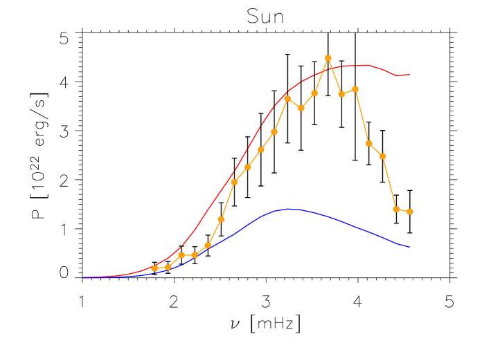
Figure 1: Rates $P$ at which solar modes with frequency n are excited. orange: excitation rates $P$ deduced from the seismic observations from the BiSon network (Chaplin et al., 1998) blue and red: excitation rates computed as explained in Sects. 2 and 3. The blue (red resp.) curve corresponds to a calculation in which $\chi_{k}$ is assumed Gaussian (Lorentzian resp. ).

5 $\alpha$ Cen A: the observations by Bedding et al (2004)

Solar-like oscillations have recently been detected in $\alpha$ Cen A by Butler et al. (2004) with the UCLES spectrograph. The identification of the modes and the determination of the mode amplitudes have been recently performed by Bedding et al. (2004). Fig. 2 presents the mode amplitudes in Doppler velocity for the l=0,1,2,3 modes which have been detected.

The authors have also derived — on the basis of the method proposed by Stello et al. (2004) — an estimation of the mode life-times for two different frequency ranges (see Table 1).

Table 1: Life-time of the modes as derived by Bedding et al. (2004) for two different frequency ranges.

Frequency range ($\mu$Hz)	1700-2400	2400-3000
Mode life-time (days)	1.4	1.3

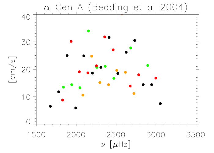
Figure 2: Amplitudes in Doppler velocity of the modes detected in $\alpha$ Cen A by Bedding et al. (2004). The green filled dots correspond to the l=0 modes, the black ones to the l=1 modes, the red ones to the l=2 modes and the orange one to the l=3 modes. Here the observed amplitudes have not been corrected for the mode visibility.

6 $\alpha$ Cen A: inferring the intrinsic amplitudes of the modes from observations

As can been seen in Fig. 2, the measured amplitudes are very scattered. Due to visibility effects, intrinsic amplitudes of l=3 modes ($I3$) are expected to be much smaller than those of l=1 ($I1$) i.e. $I3\ll I1$.

However some observed amplitudes of l=3 ($O3$) are found as large as those of l=1 ($O1$) but for a given radial order, amplitudes for l=1, l=3 modes are clearly anticorrelated as shown in Fig. 2. This suggests that the observed amplitude of a given mode l=3 can be strongly biaised by the presence of a neighborhood l=1 mode. In contrast, the pollution of the l=1 amplitude by that of a l=3 one is expected to be quite small. Neglecting this pollution effect, we sum the amplitudes of l=3 and l=1 neighboring modes of a given radial order and attribute this amplitude to l=1 mode i.e.: Since $I3\ll I1$, then $O3+O1=I3+I1\sim I1$. We next correct for the mode visibility.

We perform the same with the l=0 modes: we sum the amplitude of l=0 mode and the l=2 mode. However this determination of the amplitudes of the l=0 modes must be more biased than for the l=1 modes as the amplitudes of the l=2 modes are not so small compared with those of the l=0 modes.

Results of this determination of the intrinsic mode amplitudes are presented in Fig. 3.

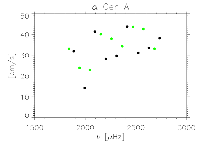
Figure 3: Inferred intrinsic amplitudes of the l=1 modes (black) and of the l=0 modes (green). The amplitudes of the l=1 modes are corrected for the mode visibility

7 $\alpha$ Cen A: comparison of the predicted excitation rates $P$ with those inferred from the observations

We derive the ’observed’ excitation rates $P$ from the intrinsic mode amplitudes (Fig. 3) and the mode life-times (Table 1) inferred from the observations according to the relation:

$$P=2\pi~{}M~{}\Gamma~{}V^{2}$$ (3)

where $\Gamma$ is the mode line-width related to the mode life-time $\tau$ (Table 1) as $\Gamma=1/\pi/\tau$, $M$ is the mode mass calculated from the mode eigenfunctions associated with the 1D stellar model of $\alpha$ Cen A and finally $V$ is the intrinsic mode amplitude (Fig. 3).

Theoretical $P$ are calculated according to Eq. (1) and as explained in Sects. 2 and 3.

Inferred and predicted mode excitation rates of $\alpha$ Cen A are presented in Fig. 4.

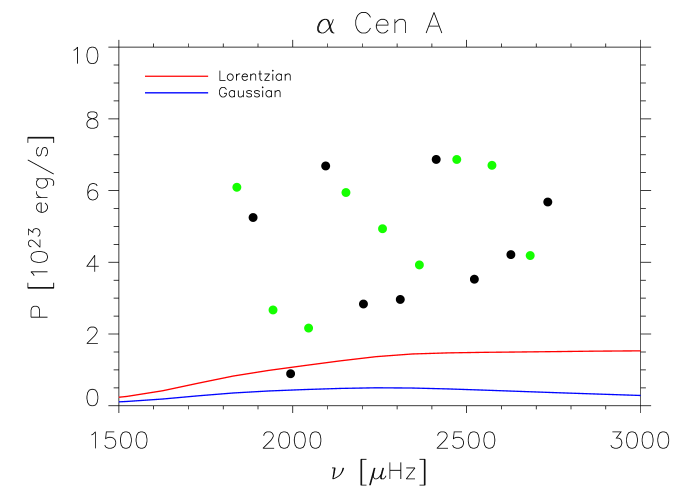
Figure 4: Filled dots correspond to the mode excitation rates derived from the inferred intrinsic amplitude (Fig. 3) of the l=0 mode (green) and the l=1 mode (black) amplitudes and the estimated mode life-times (Table 1). The blue and red curves correspond to the excitation rates computed as explained in Sects. 2 and 3. The blue (red resp.) curve corresponds to a calculation in which $\chi_{k}$ is assumed Gaussian (Lorentzian resp.).

8 Conclusion

For $\alpha$ Cen A as for the Sun, $P$ computed assuming the Lorentzian function for the eddy-time correlation function $\chi_{k}$ tend to be closer to the observations than those assuming the Gaussian function, however the quality of the data does not allow to conclude firmly about the best function for $\chi_{k}$.

In this first tentative comparison, the predictions and the observations of $\alpha$ Cen A disagree by a large amount (the inferred $P$ are very scattered: the disagreement varies by a factor 2 to 7 approximatively). This large discrepancy can either be caused by the present data quality which is not sufficient for our purpose , by the way the intrinsic amplitudes and the life-times of the modes are determined or finally attributed to the present modelling. Data of higher quality or/and more adapted data reductions are really welcome for deriving precise constraints on the p-mode excitation in $\alpha$ Cen A.

References

- Balmforth (1992) Balmforth, N. J. 1992, MNRAS, 255, 639
- Bedding et al. (2004) Bedding, T. R., Kjeldsen, H., Butler, R. P., et al. 2004, submitted to ApJ
- Butler et al. (2004) Butler, R. P., Bedding, T. R., Kjeldsen, H., et al. 2004, ApJ, 600, L75
- Chaplin et al. (1998) Chaplin, W. J., Elsworth, Y., Isaak, G. R., et al. 1998, MNRAS, 298, L7
- Chaplin et al. (1997) —. 1997, MNRAS, 288, 623
- Christensen-Dalsgaard (1982) Christensen-Dalsgaard, J. 1982, MNRAS, 199, 735
- Christensen-Dalsgaard & Berthomieu (1991) Christensen-Dalsgaard, J. & Berthomieu, G. 1991, Theory of solar oscillations (Solar interior and atmosphere (A92-36201 14-92). Tucson, AZ, University of Arizona Press, 1991, p. 401-478.), 401–478
- Christensen-Dalsgaard & Frandsen (1983) Christensen-Dalsgaard, J. & Frandsen, S. 1983, Sol. Phys., 82, 165
- Goldreich & Keeley (1977) Goldreich, P. & Keeley, D. A. 1977, ApJ, 212, 243
- Goldreich et al. (1994) Goldreich, P., Murray, N., & Kumar, P. 1994, ApJ, 424, 466
- Libbrecht (1988) Libbrecht, K. G. 1988, ApJ, 334, 510
- Samadi & Goupil (2001) Samadi, R. & Goupil, M. . 2001, A&A, 370, 136
- Samadi et al. (2001) Samadi, R., Goupil, M. ., & Lebreton, Y. 2001, A&A, 370, 147
- Samadi et al. (2003a) Samadi, R., Nordlund, Å., Stein, R. F., Goupil, M. J., & Roxburgh, I. 2003a, A&A, 404, 1129
- Samadi et al. (2003b) —. 2003b, A&A, 403, 303
- Stein (1967) Stein, R. F. 1967, Solar Physics, 2, 385
- Stein & Nordlund (1998) Stein, R. F. & Nordlund, A. 1998, ApJ, 499, 914
- Stello et al. (2004) Stello, D., Kjeldsen, H., Bedding, T. R., et al. 2004, Sol. Phys., 220, 207