Flux and energy modulation of redshifted iron emission in NGC3516: implications for the black hole mass

Abstract

We report the tentative detection of the modulation of a transient, redshifted Fe K$\alpha$ emission feature in the X-ray spectrum of the Seyfert galaxy NGC 3516. The detection of the spectral feature at 6.1 keV, in addition to a stable 6.4 keV line, has been reported previously. We find on re-analysing the XMM-Newton data that the feature varies systematically in flux at intervals of 25 ks. The peak moves in energy between 5.7 keV and 6.5 keV. The spectral evolution of the feature agrees with Fe K emission arising from a spot on the accretion disc, illuminated by a corotating flare located at a radius of (7–16) $r_{\rm g}$, modulated by Doppler and gravitational effects as the flare orbits around the black hole. Combining the orbital timescale and the location of the orbiting flare, the mass of the black hole is estimated to be (1–5)$\times 10^{7}$M_⊙, which is in good agreement with values obtained from other techniques.

1 Introduction

The Fe K$\alpha$ line is commonly observed in X-ray spectra of Active Galactic Nuclei (AGN). A narrow line at $6.4$ keV is often seen and originates most likely from distant material, such as the broad line regions or the molecular torus. A number of AGN and Galactic Black Holes Candidates (GBHCs) exhibit broad Fe emission, which is believed to originate in the innermost part of the accretion flow, where the line profile is shaped by special and general relativistic effects, such as Doppler shifts, gravitational redshift and light bending, as a result of the accreting material moving close to the speed of light and the large spacetime curvature (e.g., Fabian et al 2000; Reynolds & Nowak 2003). While the shape of the relativistic Fe line implies that the line emitting region is a few $r_{\rm g}$($=GM/c^{2}$), this does not constrain the mass of the black hole, which needs a physical unit for the emitting radius.

In addition to the major line emission around 6.4 keV, transient emission features at energies lower than 6.4 keV are sometimes observed in X-ray spectra of AGN. An early example was found in the ASCA observation of MCG–6-30-15 in 1997, which was interpreted as Fe K emission induced from a localised flare or from a narrow range of radii in the inner part of the accretion disc (Iwasawa et al 1999). More examples followed in recent years with improved sensitivity provided by XMM-Newton and Chandra X-ray Observatory (Turner et al 2002; Guainazzi et al 2003; Yaqoob et al 2003; Iwasawa et al 2004; Dovčiak et al. 2004; Turner et al 2004). These features can be attributed to an Fe K$\alpha$ line arising at a particular radius illuminated by a localised flare. If the illuminated spot is close to the central black hole, then the line emission is redshifted, depending on the location of the spot on the disc (Iwasawa et al 1999; Ruszkowski 2000; Nayakshin & Kazanas 2001; Dovčiak et al 2004).

In this context, the flare responsible for the spot illumination is most likely linked with the accretion disc via magnetic fields and is entrained with the disc orbital motion. A long-lived flare therefore orbits the central black hole with a period similar to that of the accretion disc at the radius where the flare takes place. If the sensitivity and duration of an X-ray observation are appropriate, evolution of the emission feature arising from such a spot can be tracked. When a flare survives more than one orbit, periodic signals should be observed. Combining this orbital period with the line emitting radius (in unit of $r_{\rm g}$) inferred from the line flux/energy evolution enables the black hole mass to be derived, as outlined by Dovčiak et al (2004).

The Keplerian orbital time around a $10^{7}$M_⊙ black hole (typical for Seyfert galaxies) is $\sim 10^{4}$ s at a radius of 10$r_{\rm g}$. Some of the long XMM-Newton observations last for $\sim 10^{5}$ s without interruptions, unlike for low-orbit satellites such as ASCA. Therefore a few cycles of periodic modulations of line emission induced by an orbiting spot in a Seyfert galaxy can occur within an XMM-Newton orbit. However, it is generally assumed that the sensitivity of currently available X-ray instruments is insufficient for detecting such orbital motion. Here, we apply an analysis technique, devised to search for temporal evolution of the Fe K line, to one of the XMM-Newton datasets in which such a redshifted Fe K emission feature has been reported.

2 The XMM-Newton data

We selected one of the XMM-Newton observations of the bright Seyfert galaxy NGC3516 (Observation ID: 0107460601), for which Bianchi et al (2004) reported excess emission at around 6.1 keV in addition to a stronger 6.4 keV Fe K$\alpha$ line in the time-averaged EPIC spectrum. The reasons for selecting this dataset as the primary target are as follows. NGC3516 is relatively bright in the Fe K band and the detection of the redshifted iron emission feature appears to be more robust than the other cases (Bianchi et al 2004). There is another XMM-Newton observation of NGC3516 carried out a few months later, in which the 6.1 keV feature is not present in the time averaged spectrum (Turner et al 2002; Miniutti et al 2004), indicating its transient nature. The black hole mass of a few times $10^{7}$ M_⊙ has been estimated from reverberation mapping technique (Ho 1999; Onken et al 2003) for NGC3516. With the black hole mass, a spot in the relativistic region of the accretion disc can complete a few orbits within the duration of an XMM-Newton observation (see below) if it survives, as discussed in the previous section. If the 6.1 keV feature is produced by such an orbiting spot, associated variability in the line emission is also observable. Dovčiak et al (2004) have already investigated the same dataset by dividing it into three time intervals of $\sim 27$ ks and found the ’red’ feature to be present in all the three spectra. This implies that the feature lasts at least for most of the observing duration. If it is variable, as the spot illumination model would predict, a study at a shorter time resolution is required. In the other XMM-Newton observation, which is longer than the one we have selected, although some narrow emission features have been reported (Turner et al 2002), they are seen only for a brief period and are fainter than the 6.1 keV feature in the first observation. We therefore consider the first observation more promising for a detailed line variability study over the second observation.

The observation started at 2001 April 10, 11:14 (UT), and the time in the light curves presented in this paper was measured from this epoch. We use only EPIC pn data, because of the high sensitivity in the Fe K band. Single and double events were selected for scientific analysis presented here. There are time intervals of high background at the beginning and in the last quarter of the observation. These intervals were excluded from our analysis, leaving a useful exposure time of 85 ks (of which the live time is 70 per cent due to the Small Window mode operation of the EPIC pn camera). The level of the background during the exposure was higher than its typical quiescence and fluctuated by some degree (see Fig. 1) but has little impact on the results presented below. The background fraction at the Fe K band is 4.4 per cent.

The data reduction was carried out using the standard XMM-Newton analysis package, SAS 6.0, and the FITS manipulation package, FTOOLS 5.3. The energy resolution of the EPIC pn camera at the Fe K band is $\approx 150$eV in FWHM.

The time-averaged 2–10 keV observed flux is $2.2\times 10^{-11}$ erg cm^-2 s^-1, and the absorption corrected luminosity is estimated to be $\sim 0.5\times 10^{43}$erg s^-1for the source distance of 38 Mpc ($z=0.0088$, $H_{0}=70$ km s^-1 Mpc^-1).

3 Data analysis

3.1 Continuum subtraction

The broad-band X-ray spectrum of NGC3516 is very complex, as a result of modification by absorption and reflection. Since our interest is on the behaviour of the relatively narrow feature in the Fe K band, we designed our analysis method as follows to avoid unnecessary complication: 1) The energy band is restricted to 5.0–7.1 keV, which is free from absorption which can affect energies below and above; 2) the continuum is determined by fitting an absorbed power-law to the data excluding the line band (6.0–6.6 keV), and is subtracted to obtain excess emission which is then corrected for the detector response. When determining the continuum in this way, the spectral curvature induced by much broad iron line emission (Miniutti, Iwasawa & Fabian 2004) is approximated by the effect of absorption and its contribution subtracted away together with the underlying continuum.

3.2 The excess emission map on the time–energy plane

We first investigated the excess emission at resolutions of 5 ks in time and 100 eV in energy. An image of the excess emission in the time-energy plane is constructed from individual time-intervals. The detailed procedure of this method is described in Iwasawa et al (2004). We have verified that the continuum in each spectrum is determined reliably and that the line flux measurements are robust against continuum modelling. The image suggests systematic variations taking place at the energies of the red feature (5.8–6.2 keV) at intervals of 25 ks while the 6.4 keV core remains nearly constant, although this raw digital image is only suggestive due to the low signal to noise ratio as discussed below.

In general, constructing an image is a useful way to search for events taking place in two dimensions of interest, e.g., time and energy in this case, when each event spreads across several pixels. Conversely, the events need to be appropriately over-sampled. In our excess emission map, the time scale of interest appears to be $\sim 25$ ks, oversampled by a factor of 5 in time. However, over-sampling can cause individual pixels to have insufficient statistics. The above individual 5-ks spectra have $\sim 60$ counts (uncorrected for the dead time) for the red feature at its peak and $\sim 85$ counts for the 6.4 keV core. Propagating Poisson error for the continuum subtraction gives a typical uncertainty for the red feature flux to be $\sim 40$ per cent. When the individual spectra are investigated individually, as done by the conventional spectral fitting, those errors are too large to test for flux variability.

However, as mentioned above, the events of interest take place over several pixels in the digital image, i.e., the characteristic variability frequency of the red feature appears to be larger than the noise frequency, which is equivalent to the time resolution (5 ks). When this condition is met, low pass filtering is effective in noise reduction. Therefore we applied weak Gaussian smoothing to the above image with a circular Gaussian kernel of $\sigma=0.85$ pixel (10 ks$\times$200 eV in FWHM). This kernel size was chosen so that random noise between neighbouring pixels is suppressed. This image filtering brings out the systematic variations of the red feature more clearly. The light curves of the major line core at 6.4 keV (6.2–6.5 keV) and the red feature (5.8–6.2 keV) are obtained from the filtered image. Fig. 1 shows the light curves of the excess emission in the two bands along with the broad-band (0.3–10 keV) light curve. The error of the line fluxes are estimated from extensive simulations, which are described in detail in Section 3.4, together with an assessment of the significance of the line flux variability.

Figure 1: Light curves of the source flux (upper panel), the Fe K red feature (middle panel), and the 6.4 keV line core (bottom panel). The source flux is measured in count rate in the 0.3–10 keV band with 2-ks resolution. The light curve of the background in the same energy band, normalised by the extraction area on the detector, is also shown in solid histogram. The line fluxes are measured by integrating excess emission over 5.8–6.2 keV for the red feature and 6.2–6.5 keV for the line core, obtained from the smoothed 5-ks resolution image of excess emission in the time-energy plane.

Figure 2: The folded light curve of the red feature. Two cycles are shown for clarity. One cycle is 25 ks. The same light curve obtained from the unsmoothed data is also shown in dotted line.

3.3 Line flux variability and its characteristic timescale

The red feature apparently shows a recurrent on-and-off behaviour. The peaks of its light curve appear at intervals of $\simeq 25$ ks for nearly four cycles. In contrast, the 6.4 keV line core remains largely constant, apart from a possible increase delayed from the ’on’ phase in the red feature by a few ks.

Folding the light curve of the red feature strongly suggests a characteristic interval of 25($\pm 5$) ks. Fig. 2 shows the folded light curve of the red feature, as well as the one obtained from the original unsmoothed data of the 5-ks fragments by folding on a 25 ks interval. This verifies that the apparent periodic behaviour of the red feature is not an artifact of the image filtering. However, a mere four cycles do not secure a periodicity. Whether random noise can produce spurious periodic variations such as observed at a significant probability is investigated by simulations below.

3.4 Error estimate and significance of the red feature variability

When Gaussian smoothing is applied, the independence of individual pixels is compromised (not by a great degree in our case of weak smoothing). This means that simple counting statistics no longer applies for estimating the error of the flux measurements. We therefore performed extensive simulations of the line flux measurements, as detailed below.

In each simulation run, both the 6.4 keV line-core and the red feature were assumed to stay constant at the flux observed in the time averaged spectrum throughout seventeen time-intervals. The normalisation of the power law continuum was set to follow the 0.3–10 keV light curve. From these simulated spectra, an image of the excess emission in the time–energy plane were obtained and then smoothed, from which light curves of the two line-bands were extracted, through exactly the same procedure as applied for the real data. The variance of each light curve was recorded. This process was repeated 1000 times.

Since the line flux is kept constant in each simulation, the variance of the individual light curves represents the measurement uncertainty. The mean variance of the 1000 simulations was computed and the standard deviation is adopted as the measurement error. Following this procedure, the errors of the line fluxes for the red feature and for the 6.4 keV line core are $0.36\times 10^{-5}$ ph s^-1 cm^-2 and $0.38\times 10^{-5}$ ph s^-1 cm^-2, respectively. With these errors, we can now assess the significance of the variability in the two line-bands (Fig. 1).

The $\chi^{2}$ test shows that a hypothesis of the 6.4 keV core flux being constant is acceptable. In contrast, the light curve of the red feature is not consistent with being constant with $\chi^{2}=36.0$ for 16 degrees of freedom. Because of the issue of the pixel independence, the $\chi^{2}$ value does not directly translate into a confidence level. The significance of the red feature variability can instead be estimated by comparing the $\chi^{2}$ values against a constant hypothesis for the real data and the 1000 simulations, or by comparing the variances directly. We find about 3 per cent of the simulations to exhibit variability at the same level as the real data, and therefore conclude that the variability of the red feature is significant at the 97 per cent confidence level.

Assuming now that the red feature is significantly variable, we examine how likely this is to occur on a 25-ks timescale. Folding the red feature light curve with the interval of 25 ks (Fig. 2) gives $\chi^{2}=24.5$ for 4 degrees of freedom. Due to the same limitation to the statistics mentioned above, we only take the false probability of 0.1 per cent, which would normally be inferred by the above $\chi^{2}$ value, as a target figure for $\chi^{2}$ tests, and examined what fraction of the simulated red-feature light curves exhibit similar level of periodic behaviour for assessing the significance. The simulated red-feature light curves were folded with six trial periods between 15 ks and 40 ks at a 5-ks step, and $\chi^{2}$ values for the folded light curves were recorded. We find 0.2 per cent show comparable or larger significance compared to the real data. This is however limited to the largest trial period of 40 ks. None of the 1000 simulations show comparable periodic signals to the real data for the trial periods of 35 ks or shorter. The same results were obtained from direct comparisons of variances of the folded light curves. This is because the smoothing suppresses the higher frequency (shorter time-scale) noise and allows the remaining random noise to manifest itself as spurious periodic variations only on long time scales. The above test indicates it is unlikely for random noise to produce the cyclic patterns at the intervals of 25 ks as observed, when our method is applied as for the real data analysis.

It should however be noted that this test is only against random independent noise, and does not necessarily prove the 25-ks periodicity of the line variations. If the line light curve has a ’coloured’ (e.g., red) noise spectrum, as AGN continuum emission usually does, folding tests could give large $\chi^{2}$ values (e.g., Benlloch et al 2001). However, general properties of the temporal behaviour of iron line emission in AGN are not yet known. Given the lack of knowledge of the matter, we have to make some assumptions for the noise spectrum when examining the periodicity. Two limited cases are presented below.

The power spectrum of the X-ray continuum variability of NGC3516 has been measured fairly well in a wide frequency range ($10^{-8}$–$10^{-3}$ Hz) and can be approximated by a broken power-law form (e.g., Markowitz et al 2003). The frequency range of interest is well above the break frequency at $\approx 2\times 10^{-6}$ Hz and the power spectrum density follows $\propto f^{-2}$, where $f$ is the Fourier frequency. If the same power spectrum is adopted for the iron line variability, the r.m.s. variability amplitude expected on the time scale of 25 ks is 2–3 per cent, much smaller than the error in line flux measurement. This means that the above test against random noise is valid in this case.

We further tested a case of the red noise with a large amplitude of variability using simulated light curves. 1000 light curves were simulated assuming the same power spectrum slope but a fractional r.m.s. amplitude of 35 per cent, similar to that in the red feature light curve, with the Timmer & König (1995) prescription. Gaussian noise based on the line flux measurement error (see above) was added to the light curves. We then folded the simulated light curves with the six trial periods between 15 ks and 40 ks and compared their $\chi^{2}$ values with that for the real data for significance. This comparison shows less than 2 per cent of the simulated light curves show stronger periodic signals than the real red feature light curve. While the above test suggests the probability of the 25 ks periodic signals being an artifact of red noise is low, given the crude assumptions, the inferred significance of the periodicity must be taken as an indication only. Also, with such a small number of cycles (and the limited frequency range of the noise spectrum we can examine), we draw no strong conclusion on the 25 ks periodicity.

3.5 Line profile variation

Figure 3: The Fe K line profiles during the on (filled circles) and off (open squares) phases of the red feature. The data are plotted in the form of a ratio against the best-fitting continuum. The energy scale has been corrected for the galaxy redshift ($z=0.0088$).

Using the above image and light curves as a guide, we constructed two spectra taken in a periodic manner from the ’on’ and ’off’ phases to verify the implied variability in the red feature. The line profiles obtained from the two spectra are shown in Fig. 3, which can be modelled with a double Gaussian (Table 1). The 6.4 keV core is resolved slightly ($\sim 5,000$ km s^-1in FWHM) and found in both spectra with an equivalent width (EW) of 110 eV. While the 6.4 keV core remains similar between the two, there is a clear difference in the energy range of 5.7–6.2 keV due to the presence/absence of the red feature. In the ’on’ phase spectrum, the red feature centred at $6.13^{+0.10}_{-0.07}$ keV (EW of 65 eV with respect to the continuum at the centroid energy) is evident. The line flux ratio to the 6.4 keV line core is $\simeq 0.7$. It is not detected in the ’off’ phase spectrum. The 90 per cent upper limit of the line flux given in Table 1 is the value when the same line centroid and the width of a Gaussian as in the ’on’ phase spectrum are adopted, and corresponds to $EW<20$ eV. The variability detected between the two spectra is significant at $4\sigma$. It would be unlikely to detect the variability if time intervals were chosen arbitrarily, as done by Dovčiak et al (2004).

3.6 Higher time resolution analysis

Having established the significance of the variability in the red feature, we now investigate possible time evolution of the feature at a finer time resolution. A similar image of excess emission but at a 2 ks time resolution is constructed. Then elliptical Gaussian smoothing with dispersion of $1.5\times 1.0$ pixel (7 ks$\times$250 eV in FWHM) has been applied to obtain the image shown in Fig. 4. The elliptical Gaussian kernel was chosen so as not to oversmooth the spectral resolution, which is kept to be 100 eV per pixel in the original mosaic image. Since the signal-to-noise ratio of the data in individual time intervals becomes worse, interpretations based on this image must be treated with cautions. However, further interesting behaviour of the red feature are noticed (see Fig. 4). The red feature apparently moves with time during each ’on’ phase revealed by the 5-ks resolution study: the feature emerges at around 5.7 keV, shifts its peak to higher energies with time, and joins the major line component at 6.4 keV, where there is marginal evidence for an increase of the 6.4 keV line flux (albeit only suggestive; see also the light curve in Fig. 1). This evolution appears to be repeated for the on-phases.

Table 1: The 6.4 keV core and the red feature of the Fe K$\alpha$ emission in on and off phases. The line energies are measured in the galaxy rest frame. The line fluxes are as observed and uncorrected for absorption. Errors are of the 90 per cent confidence range for one parameter of interest.

	$E$	$\sigma$	Line flux
	keV	keV	$10^{-5}$ph s-1 cm-2
Core	$6.42^{+0.02}_{-0.02}$	$0.045^{+0.020}_{-0.020}$	On: $2.9^{+0.6}_{-0.4}$	Off: $3.2^{+0.5}_{-0.5}$
Red	$6.13^{+0.10}_{-0.07}$	$0.15^{+0.25}_{-0.07}$	On: $2.1^{+1.3}_{-0.8}$	Off: $<0.7$

4 Interpretation and modelling

The detection of only four cycles is not sufficient to establish any periodicity at high significance. The 25 ks is however a natural timescale of a black hole system with a black hole mass of a few times $10^{7}$ M_⊙, as measured for NGC3516. The finding could potentially be important and, especially the evolution of the line emission, warrant a theoretical study. Here we shall assume that the 25 ks timescale is associated with the orbital motion of a corotating flare which illuminates a spot on the accretion disc, and present theoretical modelling which reproduces the saw-tooth features seen in Fig. 4. It also allows us to combine timing and spectral information for estimating the black hole mass.

Note that since a flare is not expected to last much longer than a few dynamical timescales nor be strictly periodic due to its orbital drift as the disc material spirals in (e.g. Karas, Martocchia & Subr 2001), the number of detectable cycles will be limited even in much longer observations. Flares occurring at small radii and/or black holes having small mass could provide shorter characteristic timescales. However, detectability is determined by a competition between line intensity and time resolution at a given throughput of the X-ray telescope. Line emission from smaller radii is more broadened, which would make it difficult to distinguish the line emission from the continuum.

4.1 The corotating flare model

We adopt a simple model in which a flare is located above an accretion disc, corotating with it at a fixed radius. The flare illuminates an underlying region on the disc (or spot) which produces a reflection spectrum, including an Fe K$\alpha$ line. The observed line flux and energy are both phase-dependent quantities and therefore, if the flare lasts for more than one orbital period, they will modulate periodically. Details on the expected behaviour can be found e.g. in the work of Ruszkowski (2000) and Dovčiak et al (2004).

The flare orbital period $T$ (equal to the spot period since corotation is assumed) is related to the black hole mass ($M_{\rm BH}$) and dimensionless spin ($a$) and to the radial location $r$ of the flare by the following relation (see e.g. Bardeen, Press & Teukolsky 1972)

$$T=310~{}[~{}a+(~{}r/r_{g}~{})^{3/2}~{}]~{}M_{7}\quad{\mathrm{[\,seconds\,]}}\ ,$$ (1)

where $M_{7}$ is the black hole mass in units of $10^{7}\,M_{\odot}$. Hereafter, by radial location $r$ we mean the flare distance from the black hole axis as measured in the equatorial plane. It is clear that if $T$ and $r$ can be inferred from observations, Eq. (1) provides an estimate of the black hole mass. Assuming that the observed 25 ks timescale corresponds to the orbital period, we now model the data and derive an estimate of $r$ that will constrain $M_{\rm{BH}}$ in NGC 3516.

4.2 Constraints on emission radius and black hole mass

We consider a corotating flare which has a power-law spectrum with photon index of $\Gamma=1.8$ (typical for Seyfert 1 galaxies) and emits isotropically at a constant flux in its proper frame. The disc illumination is computed by integrating the photon geodesics in a Kerr spacetime from the flare to the disc, and is converted to local emissivity (see e.g. George & Fabian 1991). Then, the observed emission line profile is computed through the widely used ray–tracing technique (see Miniutti et al 2003 and Miniutti & Fabian 2004 for more details).

Figure 4: The smoothed excess emission map on the time-energy plane. The pixel size is 2 ks in time and 100 eV in energy. The energy scale is as observed. The flux of the excess emission is indicated by the false colour, in the unit of photons/2000-s/cm². The value of 0.02 corresponds roughly to 10 counts (uncorrected for the dead time due to the EPIC operation in Small-Window mode).

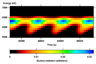
Figure 5: The smoothed theoretical time–energy map of the emission feature. The time resolution is enforced by dividing the flare orbit into $13$ intervals. By assuming an orbital period of $26$ ks (consistent with the measured period of $25\pm 5$ ks), each interval corresponds to $2$ ks. See text for details on the model parameters. No noise has been added to the theoretical results.

The free parameters of our model are the flare location, specified by $r$ and the height above the accretion disc ($h$), the accretion disc inclination $i$, the emission line rest–frame energy, and the inner disc radius. We assume a maximally rotating Kerr black hole with spin parameter, $a=0.998$. Note that the difference in the orbital period between a maximally rotating and a non-rotating black hole is smaller than the uncertainty of the period (20 per cent) when $r>3$ $r_{\rm g}$, for which our results would be insensitive to the spin of the black hole. Our assumption on the spin parameter needs to be verified once a lower limit on the flare radial position has been obtained.

Figure 6: A comparison between the observed (solid line) and predicted (dotted line) light curves in the 6.0–6.2 keV (upper panel) and 5.8–6.0 keV (lower panel) bands, obtained from the excess maps in Fig. 4 and Fig. 5. This demonstrates the level of match between the two. The model describes the amplitudes and delays of the emission feature as a function of time reasonably well, given the quality of the data.

The variation of energy and flux of the emission feature also depends on the assumed disc inclination. We have analysed all the BeppoSAX and XMM-Newton datasets available and found the Fe K line profiles are all consistent with $i=30^{\circ}\pm 10^{\circ}$. The range of inclination is in good agreement with previous results based on the ASCA data (Nandra et al 1997; Nandra et al 1999; Čadež et al 2000).

We have computed the evolution of Fe K emission induced by an orbiting flare and simulated time-energy maps with the same resolution and smoothing as in the excess emission map of Fig. 4. A constant, narrow $6.4$ keV core representing the Fe K$\alpha$ line from distant material is also added. As pointed out by Dovčiak et al (2004), the faint, broad part of the line profile has little contrast against the continuum and is likely missed in the observed excess map. To simulate this effect, we set a threshold below which line emission is assumed to have null intensity. The threshold is an additional parameter of the model and its adopted range is 30–40 per cent of the maximum amplitude of the emission feature during the orbital period.

Given the quality of the observed map in Fig. 4 and the simplified situation assumed in our model, an exact match of the simulated map with the observation is not to be expected (nor to be looked for). However, we have explored the parameter space, aiming to reproduce the key features as outlined below and constrain the maximum range of $r$ allowed by the data. The key features we identified are the followings: a) the emission has a skewed form in the time–energy map (no significant emission is seen below 6.1 keV during the ‘off’ phase); b) during the ‘on’ phase, the emission appears at $\sim 5.7$ keV, moves with time to join the narrow 6.4 keV emission and reaches the maximum energy of about $6.5$ keV; c) the maximum-to-minimum flux ratio of the feature in this phase is about 2; and d) the ‘on’ and ‘off’ phases have approximately equal durations.

The lack of emission below 6.1 keV during the ‘off’ phase, which makes the saw-tooth pattern of the excess map (Fig. 4), is the most notable difference from the predictions in the previous work (Nayakshin & Kazanas 2001; Dovčiak et al 2004). If the spot size is small, the emission line is always narrow during the orbital period, and the ‘off’ phase shows a decay both in energy and flux, resulting in an almost symmetric pattern to the rising ‘on’ phase, especially when the inclination is $\sim 30^{\circ}$. In contrast, in our model, the disc illumination is computed self-consistently and the spot size is related to the height of the illuminating source (i.e., flare): the higher the flare, the larger the spot (see also Ruszkowski 2000 for other relativistic effects mainly due to light bending). This causes the observed line profile to be broadened. Therefore when a flare is located higher than a certain height (typically $h\mathrel{\hbox{\hbox to0.0pt{\hbox{\lower 4.0pt\hbox{$\sim$}}\hss}\hbox{$>$}}}3~{}r_{g}$, depending on $r$), the broadened line emission becomes undetectable because of the lack of the contrast to the underlying continuum. This occurs at a phase when the flare is on the near receding side of the disc, which corresponds to the ’off’ phase, and explains the skewed form of the excess emission in Fig. 4.

Fig. 5 shows one of the theoretical time-energy maps that we consider to be in reasonable agreement with the observed map because they reproduce the key features mentioned above. This particular example assumes a flare with $(\,r\,,\,h\,)=(\,9\,,\,6\,)~{}r_{g}$, the rest-frame line energy of 6.4 keV, a disc inclination of $20^{\circ}$, an inner disc radius of 1.24 $r_{\rm g}$, and a detection threshold of 37 per cent. The normalisation of the excess emission in the theoretical map is adjusted so that the Fig. 5 can be compared with Fig. 4 directly. In Fig. 6, light curves in the two selected bands, obtained from the smoothed observed (Fig. 4) and simulated (Fig. 5) maps are shown to illustrate the degree of agreement between the model and the observation.

By applying the above procedure we find for the flare radius

$$7~{}r_{g}\mathrel{\hbox{\hbox to0.0pt{\hbox{\lower 4.0pt\hbox{$\sim$}}\hss}\hbox{$<$}}}r\mathrel{\hbox{\hbox to0.0pt{\hbox{\lower 4.0pt\hbox{$\sim$}}\hss}\hbox{$<$}}}16~{}r_{g}\ .$$ (2)

Radii larger than $16~{}r_{g}$ are ruled out because 1) the amplitude of flux variation during the ‘on’ phase becomes too large; 2) the ‘on’ phase lasts longer than the ‘off’ phase; and 3) substantial emission below 6.1 keV appears during the ‘off’ phase above the detection threshold. If the orbital radius is smaller than $7~{}r_{g}$, the opposite trend is seen. Some uncertainty comes from the presence of the narrow 6.4 keV line which blends with the moving feature at energies above 6.2 keV. Note that, since the minimum radius we find is larger than $3~{}r_{g}$, the orbital time is insensitive to our assumption of the maximally-rotating Kerr spacetime.

Together with $T=(~{}25\pm 5~{})$ ks, and by using Eq. (1), the flare radius translates to a black hole mass in NGC 3516:

$$1.0\times 10^{7}~{}M_{\odot}\mathrel{\hbox{\hbox to0.0pt{\hbox{\lower 4.0pt\hbox{$\sim$}}\hss}\hbox{$<$}}}M_{\rm{BH}}\mathrel{\hbox{\hbox to0.0pt{\hbox{\lower 4.0pt\hbox{$\sim$}}\hss}\hbox{$<$}}}5.0\times 10^{7}~{}M_{\odot}\ .$$ (3)

5 Discussion and Conclusions

We study the variability of a transient emission feature around 6 keV, of which detection has been reported previously in the time averaged X-ray spectrum of NGC3516. The feature appears to vary systematically both in flux and energy on a characteristic timescale of 25 ks. On comparing with extensive simulations, the variability is found to be significant at the 97 per cent confidence level, and the probability for the variations to occur cyclically as observed purely due to random noise is very low (see Section 3.4).

The flux and energy evolution of the red feature is consistent with being Fe K$\alpha$ emission produced by an illuminated spot on the accretion disc and modulated by Doppler and gravitational effects. Modelling the observed X-ray data with a relativistic disc illuminated by a corotating flare above it constrains the radial location of the flare to be $r=(7-16)~{}r_{g}$. This is combined with the orbital period to provide an estimate of the black hole mass in NGC 3516 which is $M_{\rm{BH}}=(1-5)\times 10^{7}~{}M_{\odot}$.

One caveat is any weak continuum variation correlated with the line variation. Since the flare is assumed to corotate with the disc, its direct emission should also produce modulation in the continuum in roughly the same way as the red feature. Ideally, this constraint should be obtained from the ionizing flux of the Fe K line, i.e., the continuum flux above 7.1 keV, but because of the poor signal to noise ratio of the light curve in those energies, the 0.3–10 keV band light curve (Fig. 1) is used instead. If the spectrum of the flare is harder than the total continuum emission, the limit given below would increase. The best constraint is obtained from the second and third ’on’ phases where the continuum light curve is relatively flat. Excess flux increases during those periods are of the order of 5 per cent, which represents an upper limit on the continuum modulation. Since the line flux of the red feature is a small fraction ($8\pm 5$ per cent on average) of that of the total broad Fe K emission, the relative contribution of the flare, which produces the red feature, to the total continuum flux is accordingly small, and the line flux ratio gives an estimate of that. Based on the estimate, the expected variability amplitude in the total light curve due to the modulation of the orbiting flare is computed for the range of flare radius and inclination of the disc derived above. It ranges over 3–19 per cent, which contains the observed limit towards the lower bound. The amplitude is smaller when the flare radius is larger and the inclination is smaller. We note the above estimate assumes other X-ray sources above the disc are entirely static. Other short-lived flares occuring at different radii may mask the continuum modulation.

The corotaing flare model is perhaps the simplest explanation for the evolution of the red feature, but there may be other models which do not invoke accompanied continuum modulation. If the red feature is related to a non-axisynmetric (e.g., spiral) structure on the disc with high emissivity, such as that resulted from density and ionzation perturbations or magnetohydrodynamic turbulance considered by Karas et al (2001) and Armitage & Reynolds (2003), respectively, then the line flux modulates as the structure orbits around but can be independent from the illuminating source.

Our result on $M_{\rm BH}$ is complementary to those from the reverberation mapping technique which are based on emission from clouds much far away from a central hole and unlikely to see those clouds to complete a whole orbit in a reasonable time. The estimates of $M_{\rm{BH}}$ in NGC 3516 from reverberation mapping lie in the range between $1\times 10^{7}~{}M_{\odot}$ and $4\times 10^{7}~{}M_{\odot}$. The most recent result obtained by combining the H$\alpha$ and H$\beta$ emission lines is $(1.68\pm 0.33)\times 10^{7}~{}M_{\odot}$ (Onken et al. 2003), while the previous analysis based on H$\beta$ alone gave $2.3\times 10^{7}~{}M_{\odot}$ (Ho 1999; no uncertainty is given). It is remarkable that our estimate of the black hole mass in NGC 3516 is in excellent agreement with the above results. Although the systematic flux and energy variability we report here is only tentative, the above agreement supports our interpretation.

Our results indicate that present X-ray missions such as XMM–Newton are close to probing the spacetime geometry in the vicinity of supermassive black holes if their observational capabilities are pushed to the limit. Future observatories such as XEUS and Constellation-X, which are planned to have much larger collecting area at $6$ keV, will be able to exploit this potential and map the strong field regime of general relativity with great accuracy.

References

- (1) Armitage P.J., Reynolds C.S., 2003, MNRAS, 341, 1041
- Bardeen, Press & Teukolsy (1972) Bardeen J.M., Press W.H., Teukolsky S.A., 1972, ApJ, 178, 347
- (3) Benlloch S., Wilms J., Edelson R., Yaqoob T., Staubert R., 2001, ApJ, 562, L121
- Bianchi et al. (2004) Bianchi S., Matt G., Balestra I., Guainazzi M., Perola G.C., 2004, A&A in press, astro-ph/0404308
- Čadež et al. (2000) Čadež A., Calvani M., di Gioacomo C., Marziani P., 2000, New Astr., 5, 69
- Dovčiak et al. (2004) Dovčiak M., Bianchi S., Guainazzi M., Karas V., Matt G., 2004, MNRAS, 350, 745
- Fabian et al. (2000) Fabian A.C., Iwasawa K., Reynolds C.S., Young A.J., 2000, PASP, 112, 1145
- George & Fabian (1991) George I.M., Fabian A.C., 1991, MNRAS, 249, 352
- Guainazzi (2003) Guainazzi M., 2003, A&A, 401, 903
- Ho (1999) Ho L.C., 1999, in Observational Evidence for Black Holes in the Universe, 157, ed. K. Chakrabarti (Kluwer, Dordrecht)
- Iwasawa et al. (1999) Iwasawa K., Fabian A.C., Young A.J., Inoue H., Matsumoto C., 1999, MNRAS, 306, L19
- Iwasawa et al. (2004) Iwasawa K., Fabian A.C., Vaughan S., Miniutti G., 2004, MNRAS, submitted
- Karas, Martocchia & Subr (2001) Karas V., Martocchia A., Subr L, 2001, PASJ, 53, 189
- (14) Markowitz A., et al, 2003, ApJ, 593, 96
- Miniutti et al. (2003) Miniutti G., Goyder R., Fabian A.C., Lasenby A.N., 2003, MNRAS, 344, L22
- Miniutti & Fabian (2004) Miniutti G., Fabian A.C., 2004, MNRAS, 349, 1435
- Miniutti, Iwasawa & Fabian (2004b) Miniutti G., Iwasawa K., Fabian A.C., 2004, MNRAS, in prep.
- Nandra et al. (1997) Nandra K., George I.M., Mushotzky R.F., Turner T.J., Yaqoob T., 1997, ApJ, 477, 602
- Nandra et al. (1999) Nandra K., George I.M., Mushotzky R.F., Turner T.J., Yaqoob T., 1999, ApJ, 523, L17
- Nayakshin & Kazanas (2001) Nayakshin S., Kazanas D., 2001, ApJ, 553, 885
- Onken et al. (2003) Onken C.A., Peterson B.M., Dietrich M., Robinson A., Salamanca I.M., 2003, ApJ, 585, 121
- Reynolds & Nowak (2003) Reynolds, C.S., Nowak M.A., 2003, PhR, 377, 389
- Ruszkowski (2000) Ruszkowski M., 2000, MNRAS, 315, 1
- (24) Timmer J., König M., 1995, A&A, 300, 707
- Turner et al. (2002) Turner T.J. et al., 2002, ApJ, 574, L123
- Turner, Kraemer & Reeves (2002) Turner T.J., Kraemer S.B., Reeves J.N., 2004, ApJ, 603, 62
- Yaqoob et al. (2003) Yaqoob T., George I.M., Kallman T.R., Padmanabhan U., Weaver K.A., Turner T.J., 2003, ApJ, 596, 85