A Parameter Study of Type II Supernova Light Curves Using
6 M_⊙ He Cores

Abstract

Results of numerical calculations of Type II supernova light curves are presented. The model progenitor stars have 6 $M{{}_{\odot}}$ cores and various envelopes, originating from a numerically evolved 20 $M{{}_{\odot}}$ star. Five parameters that affect the light curves are examined: the ejected mass, the progenitor radius, the explosion energy, the ⁵⁶Ni mass, and the extent of ⁵⁶Ni mixing. The following affects have been found: 1) the larger the progenitor radius the brighter the early–time light curve, with little affect on the late–time light curve, 2) the larger the envelope mass the fainter the early light curve and the flatter the slope of the late light curve, 3) the larger the explosion energy the brighter the early light curve and the steeper the slope of the late light curve, 4) the larger the ⁵⁶Ni mass the brighter the overall light curve after 20 to 50 days, with no affect on the early light curve, 5) the more extensive the ⁵⁶Ni mixing the brighter the early light curve and the steeper the late light curve. The primary parameters affecting the light curve shape are the progenitor radius and the ejected mass. The secondary parameters are the explosion energy, ⁵⁶Ni mass and ⁵⁶Ni mixing. I find that while in principle the general shape and absolute magnitude of a light curve indicate a unique set of parameters, in practice it is difficult to avoid some ambiguity in the parameters. I find that the nickel–powered diffusion wave and the recombination of helium produce a prominent secondary peak in all our calculations. The feature is less prominent when compositional mixing, both ⁵⁶Ni mixing and mixing between the hydrogen and helium layers, occurs. The model photospheric temperatures and velocities are presented, for comparison to observation.

1 Introduction

Type II supernovae (SNe) are classified by the presence of H in their spectra and sub-classes are based on their observed light curves. They are most likely caused from the gravitational collapse of a main sequence stars with M $>$ 8-10 $M_{\odot}$. The differences in Type II light curves was first pointed out by Pskovskii (1978) by introducing the beta parameter which resulted in a continuous classification based on the slope of the light curve. Another study showed that light curves can be differentiated into two distinctive sub-classes, plateaus and linears (Barbon et al.,, 1979). Pata et al. (1994), using a multivariable factor analysis, introduced a new classification based on an absolute peak magnitude vs. $\beta_{100}$ graph resulting in three sub-classes; Bright (includes both plateaus and linears), Normal (includes both plateaus and linears), and Faint.

Good observations of Plateau SNe such as SN 1969L, SN 1987A, SN 1993J and recently SN 1999em and SN 1999gi are usually followed by extensive theoretical light curve (LC) studies. After SN 1969L LC calculations correctly predicted features found in the observations (Grassberg and Nadyozhin,, 1969, 1976; Grassberg et al.,, 1971). Later more refined analytic treatments and hydrodynamical codes were developed (Falk and Arnett,, 1977; Chevalier and Klein,, 1979) and applied to red supergiant progenitors. Litvinova and Nadyozhin, (1983) conducted a numerical parameter study to examine how the ejected mass, progenitor radius, and explosion energy affect the plateau duration and magnitude of the light curve and photospheric velocity of material. They showed that relations between explosion energy, envelope mass, and progenitor radius can be obtained from observations of plateau duration, the absolute magnitude and the photospheric velocity. We are currently preparing a paper investigating a comparison between supernovae of evolved numerical stars and polytrope stars using the method (Young and Johnson,, 2004).

More recently Hamuy (2003) has conducted an observational parameter study based on properties of 24 type II supernova spectra and light curves. The author finds correlations between Ni mass and plateau luminosity, large ranges in all parameters, and a continuum in the parameter space for type II plateaus. Other studies of type II plateaus have found similar results. One study presents a technique of determining Ni mass based on H$\alpha$ luminosity at nebular phases (Elmhamdi et al.,, 2003). As mentioned above we will be publishing a paper comparing the light curves of numerical model explosions to those presented in Litvinova and Nadyozhin, (1983, 1985) and compare the least-squares fit formulas in their paper to those found in this study (Young and Johnson,, 2004).

Many papers on SN 1987A have been published on LC modeling and references can be found in review articles (Arnett et al.,, 1989; Imshennik and Nadyozhin,, 1989). In order to obtain a good fit to SN 1987A variations in envelope masses, explosion energies, progenitor radii, and mixing of both hydrogen-helium and ⁵⁶Ni were explored but only in a limited parameter space (Woosley,, 1988; Nomoto et al.,, 1991; Shigeyama and Nomoto,, 1990; Utrobin,, 1993). Podsiadlowski et al. (1992) in an attempt to find variations in Type II progenitors examined binary systems and showed it is possible to find many different scenarios. Hsu et al. (1993) , using hydrodynamical models, examined Type II light curves by varying the envelope mass and explosion energy.

The unusual LC of 1993J produced interest in possibly new progenitors. Many studies of SN 1993J conclude that the progenitor was a 4 $M_{\odot}$ helium core with an envelope of about 0.2 $M_{\odot}$ of hydrogen, a radius of about 300 R_⊙ and belonged to a binary system (Young et al.,, 1995; Shigeyama et al.,, 1994; Nomoto et al.,, 1993; Podsiadlowski et al.,, 1993; Bartunov et al.,, 1994). A more extensive study on SN 1993J was conducted by Blinnikov et al. (1998) comparing calculations from two different numerical codes by analyzing the evolution and explosion of the progenitor. Young et al.(1995), using the cepheid distance to M81 (Freedman et al., 1994), found a lower limit to the Ni mass of 0.1 $M_{\odot}$. Using the X-ray light curve Suzuki and Nomoto (1995) found a upper limit to explosion energy to be 1$\times 10^{51}$ ergs. Recently the massive companion star for SN 1993J was observed 10 years after the explosion, confirming the suggested binary system with two similar mass stars (Maund et al.,, 2004). Superior observations of supernova progenitors are now starting to constraining model progenitors and making light curve analysis more precise, e.g. SN 2001du Smartt et al., (2003).

Two well observed SNe 1999em and 1999gi have been extensively studied. The nature of the progenitor of SN1999em is constrained to be around 12 $M_{\odot}$(Smartt et al.,, 2002). The upper mass limit of SN 1999gi has been revised to 15 $M_{\odot}$. Both these progenitor masses are similar to that found in numerical fits to the light curves of SN 1999em and SN 1999gi (Young et al.,, 2002, 2004). As observations become more complete type II plateaus have a potential to be used as distance indicators. The distances to both SNe were found by using the expanding photosphere method (EPM) (Leonard and others, 2002a, ; Leonard and others, 2002b, ). Other studies examined type IIs as possible distance indicators using expansion velocities that correlate with the bolometric luminosity (Hamuy and Pinto,, 2002).

Young and Branch (1989) compared observed Type IIp light curves on an absolute magnitude scale and found a large spread in absolute magnitude, their plateau duration, and slope of the tails, attributing it to differences in the physical properties of the progenitor. These studies indicate that the parameter space is quite large for the progenitor of Type II SNe and it is difficult to say what type of progenitor will explode or not. What is needed is a parameter study that encompasses all variables and all combinations, but this is unfeasible. Therefore the aim of this and future studies is to have a standard SN model with parameters that are consistent with knowledge of progenitor stars, explosion mechanisms, and hydrodynamics. It is then of interest to see if all observed light curves can fit into this model and how far in parameter space they deviate from the standard model. In this study the standard model is a 20 $M_{\odot}$ main sequence star that has gone through a wind mass loss of 2 $M_{\odot}$, left a neutron star of 1.4 $M_{\odot}$, thus ejecting about 16 $M_{\odot}$ with a progenitor radius of 3$\times 10^{13}$ cm. The energetics of the simulation has a total energy of 1$\times 10^{51}$ ergs or 1 foe (ten to the fifty one ergs) and ejects 0.07 $M_{\odot}$ ⁵⁶Ni mixed throughout the 6 $M_{\odot}$ He core. The standard model is similar to SN 1987A except for the larger radius and less extensive mixing. In this paper the parameter space around this model is explored.

In this paper I show the results of how varying each parameter can influence the shape and absolute magnitude of Type II light curves out to 400 days. The five parameters explored in this study are; the progenitor radius, envelope mass, explosion energy, ⁵⁶Ni mass, and ⁵⁶Ni mixing. All light curves calculated in this paper use the numerically evolved 20 $M{{}_{\odot}}$  main sequence model with a 6 $M_{\odot}$ helium core from Woosley and Weaver (1980). The envelope parameters, mass and radius, are varied using homology transformations (section 2). The models are then exploded in a one dimensional, flux-limited hydrodynamical code with a simple prescription for gamma-ray deposition (section 3). The bolometric light curves are calculated and plotted on an absolute magnitude scale (section 4). The results are discussed in section 5.

2 Initial Models

For the initial models of all explosions I use the 6 $M{{}_{\odot}}$ helium core from Woosley and Weaver (1980) , originally a 20 $M{{}_{\odot}}$ main sequence star. The envelope mass and radius are subsequently modified in a systematic way. A total of 8 models were constructed that are identified by a specific mass and radius (Table I). In this study three different envelope masses were used producing total masses of 8, 12, and 16 $M{{}_{\odot}}$. For each envelope mass, three different radii where used 43 R_⊙ ($3\times 10^{12}$ cm) , 430 R_⊙ ($3\times 10^{13}$ cm), and 4300 R_⊙ ($3\times 10^{14}$ cm). The original H rich envelope was modified by homologous transformations to give the various masses and radii (Schwarzschild,, 1958; Chandrasekhar,, 1939).

For a homologous transformation in radius:

$$R^{\prime}=xR.$$

where R is the old radius, R^′ is the new radius, and $x$ is the percent changed. For a homologous transformation in mass :

$$\frac{1-\beta_{1}}{\mu_{1}^{4}\beta_{1}^{4}}=\frac{1-\beta_{o}}{\mu_{o}^{4}\beta_{o}^{4}}\left(\frac{M_{1}}{M_{o}}\right)^{2}$$

where $\beta_{o}$ and $\beta_{1}$ are the ratio of the gas pressure to the total pressure for the star before and after the homologous transformation. $M_{o}$ and $M_{1}$ are initial and final mass, and $\mu_{o}$ and $\mu_{1}$ are the mean molecular weights for the initial and final configuration. Following either of these calculations the remaining physical variables, $\rho$ and T, must be solved to ensure hydrostatic equilibrium. The homologous transformation is performed on the hydrogen envelope only and then matched to the He core. The core and various envelopes were then re-zoned to ensure a continuous density, temperature and radius. Eight progenitor models in all were constructed for this study each having 170 zones in order to have consistent results for opacity floors (opacity minimum) and gamma-ray deposition which are used to calculate zone dependent quantities like the photosphere and the gamma-ray contribution to the luminosity (see section 3). The innermost 1.4 $M_{\odot}$ is assumed to form a neutron star and is removed from the core, but set as an inner boundary condition in the explosions.
The constructed models are in hydrostatic equilibrium but not necessarily in radiative equilibrium. This should not be a problem since the shock moves through the star in 6 to 240 hours. Radiative equilibrium is important concerning the validity of the model stars representing real stars, but the point of this study is to compare various simple models and see how the LC responds.
Three different final explosion energies, $1\times 10^{51}$, $2\times 10^{51}$, and $3\times 10^{51}$ ergs are obtained by artificially placing the required energy, divided between kinetic and thermal, in the first few mass zones. This procedure is justifiable since the explosion mechanism for Type II SNe is beyond the scope of this paper. Furthermore, the type of shock is only important in the nucleosynthesis (Aufderheide 1991) which is not included in our study.

3 Numerical Method and Gamma-Ray Deposition

The radiation-hydrodyanmics code given to the author (Wheeler,, 1992; Sutherland and Wheeler,, 1984) contains the following attributes; spherically symmetric, 1-D, Lagrangian, flux-limited code which uses pseudo-viscosity and determines opacities calculated for hydrogen, helium, and oxygen rich layers. Modifications included a geometric dilution model for gamma-ray deposition, and updated opacity tables (Young,, 1994). Rayleigh-Taylor mixing and nuclear reactions are not included in the calculations. The Rosseland mean opacities are tabulated as functions of composition, temperature, and density,assuming local thermodynamic equilibrium. Two effects not included in the Rosseland mean are line opacities and non-thermal excitation or ionization from gamma rays. In order to account for these affects an opacity minimum (opacity floor) is set at 0.25 cm² g^-1 for the helium rich core and 0.01 cm² g^-1 for the hydrogen rich envelope.
The LC calculation is done in two steps, first the hydrodynamics is calculated, then in a second step the gamma-ray deposition is included in the computation. The prescription for absorbed gamma rays requires calculating a deposition function following Sutherland and Wheeler (1984) at interval times of 3.5$\times 10^{6}$ sec from 0 to 400 days. The deposition function calculates the diffusion of gamma-rays from the location they are produced to regions outside the Ni distribution, including gamma-rays escaping the ejecta. In the first step one obtains the time evolution of density and volume of the ejecta that is necessary to calculate the absorbed gamma rays.

The energy produced by the gamma rays is not enough to affect the hydrodynamics and thus is not necessary to be included in the primary run. This saves computation time, avoiding a calculation of the deposition function at each time step.
The ⁵⁶Ni mass is varied using 3 different masses of 0.035, 0.07, and 0.14 $M{{}_{\odot}}$ which are mixed to three different regions; less than 0.3 $M{{}_{\odot}}$, 6 $M{{}_{\odot}}$ (He core), and 11 $M{{}_{\odot}}$ (core plus half the envelope, 7 $M{{}_{\odot}}$ for model G). The Ni distribution is a step function resulting in a uniform spherical distribution of ⁵⁶Ni. As the ejecta becomes thin, the gamma rays deposit energy in a symmetric sphere outside the ⁵⁶Ni distribution. The mixing of ⁵⁶Ni is artificial since we are not mixing the composition along with it, but the goal of this study is not to create a rigorous model, only to explore the major parameters that influence the LC. However it has been shown that the mixing of H into the He layer does affect the LC as seen in SN1987A (Arnett et al.,, 1989; Imshennik and Nadyozhin,, 1989). The energy produced by the decay of ⁵⁶Ni and ⁵⁶Co is

$$S(t_{days})=\frac{3.4\times 10^{11}e^{-t/\tau_{Ni}}}{\tau_{Ni}}+\frac{7.5\times 10^{11}}{\tau_{Co}-\tau_{Ni}}(e^{-t/\tau_{Co}}-e^{-t/\tau_{Ni}})\ ergs\ g^{-1}s^{-1}$$ (1)

where S is the amount of energy per gram per second produced from the Ni-Co-Fe decay, t is time in days, $\tau_{Ni}$=8.8 days and $\tau_{Co}$=113.6 days and the amount being deposited in the SN ejecta ($S_{dep}$) is

$$S_{dep}(t_{days})=Dep\times S(t_{days})\ ergs\ g^{-1}s^{-1}$$ (2)

where Dep is the deposition function. In it is useful to introduce a gamma-ray “photosphere” (hereafter gammasphere), similar to how the actual photosphere is defined. This is taken to be $\tau_{\gamma}$ = 2/3, found by integrating the gamma-ray cross-section 0.06 cm² g^-1 and the net electron mole fraction Y_e.
The gamma rays are produced from the decay of ⁵⁶Ni to ⁵⁶Co, releasing photons with an average energy of 1.75 MeV, and ⁵⁶Co to ⁵⁶Fe, releasing photons with an average energy of 3.61 MeV, and positrons with an average kinetic energy of 0.12 MeV.
The optical photosphere is defined to be where $\tau$=2/3, integrating inward from the surface. The optical opacities are calculated and tabulated using bound-bound, free-free and bound-free transitions for multi-level atoms of H, He, C, O, Si, Fe. These tables were made for calculations where the H envelope was metal deficient, such as SN 1987A. This is not a problem in LC calculations because in the region where the optical depth is high most of the opacity comes from electron scattering and the metal lines are an insignificant contribution. In the optically thin regions the opacity is so low that the contribution of metal lines to the opacity is small. Plus the metalicity of progenitors is unclear, SNe found far from the nucleus in large galaxies with steep metalicity gradients most likely will have low metalicity envelopes.
The total luminosity (L) at any time is defined as the luminosity at the photosphere ($L_{PHOTO}$) plus the energy produced by the deposition of gamma rays above the photosphere which is assumed to add to the bolometric luminosity.

$$L=L_{PHOTO}+\int^{R}_{r_{photo}}m(r)S_{dep}(r)dr.$$ (3)

Where $r_{photo}$ is the position of the photosphere, $R$ is the radius of the ejecta, $m(r)$ is the mass at radius $r$, and $S_{dep}$ is energy per gram per second deposited by gamma rays at radius $r$. At late times when the gammasphere has receded through the ejecta the energy source of the LC is just the spontaneous release of energy deposited by the decay of Ni-Co-Fe. The absolute magnitude light curves are calculated following Swartz et al. (1991),

$$M_{bol}=-18.793-2.5log_{10}L_{43}$$ (4)

Where $M_{bol}$ is the absolute bolometric magnitude and $L_{43}$ is the total luminosity in units of $1\times 10^{43}$ ergs. Visual and blue light curves are calculated by assuming a blackbody at the effective temperature integrated over the V and B response curve given in Azusienis and Straizy (1969) . The photospheric temperature, T_photo, is defined by

$$T_{photo}=max\left\{{\left(\frac{L}{4{\pi}R^{2}_{photo}\sigma}\right)}^{0.25},4500\right\}$$ (5)

following Swartz et al. (1991). Where $L$ is the total luminosity and $R_{photo}$ is the photospheric radius. Finally the velocity at the photosphere, V_photo is the velocity of the material at the the photosphere.

4 Results

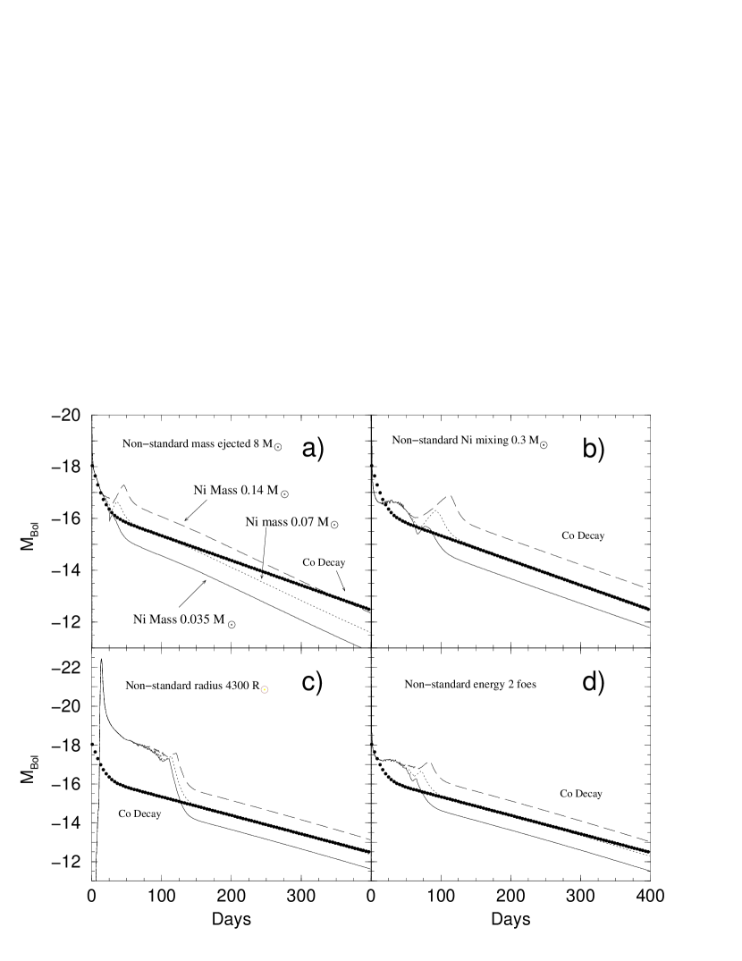
Figure 12: Absolute magnitude bolometric light curves showing the variations of the Ni mass with different constant values of the parameters. For reference the spontaneous luminosity of the Ni-CO-Fe decay for 0.07 M_⊙ Ni is shown. Plot a) shows the affect of Ni mass with the ejected mass reduced to 8 M_⊙ (variations of model G). Plot b) Shows the light curves of the same models as in figure 10 except the Ni mixing for all three models is $<$ .3 M_⊙. Plot c) shows the affect of Ni mass with the progenitor radius is increased to 4300 R_⊙ (variations of model C). Plot d) Shows the light curves of the same models as in figure 10 except the explosion energy for all three models is increased to $2\times 10^{51}ergs$.

The models A-H (Table I) were constructed in order to easily compare the behavior of one parameter while holding the other parameters constant. The standard model is model B (M = 16 M_⊙, R = 430 R_⊙) with E = $1\times 10^{51}$ ergs, M_Ni = 0.07 M_⊙, and Ni mixing throughout the 6 M_⊙ core. These are similar to the values of SN 1987A except with a larger radius, taking into consideration that SN 1987A might have had a nonstandard radius. Thus I take the standard model as having the most average values around which the parameters are varied. The 5 parameters are the progenitor radius, envelope mass, explosion energy, mass of ⁵⁶Ni, and ⁵⁶Ni mixing. All LC graphs are plots of absolute magnitude versus time in days and all calculations proceed to 400 days and include the observed LC of SN 1987A for comparison (Catchpole and others,, 1987). Figs. 1-3 show the affects of progenitor radius, Figs. 4-6 show the affects of ejected mass, Figs. 7-9 show the affects of explosion energy, Figs. 10-12 show the affects of Ni mass, Figs. 13-15 show the affects of Ni mixing. Figs. 1, 4, 7, 10, and 13 show bolometric and visual light curves, and photospheric temperature and velocity for each of the “affects of” series. Figs. 2, 5, 8, 11, and 14, show the density and temperature profiles for each of the “affects of” series at times 0, 36 hours, and 47 days. Also shown is the final velocity profile and the luminosity versus mass at times 94, 189, and 379 days. Figs. 3, 6, 9, 12, and 15, show the affects on the LC at different values of the parameters that are held constant for each of the “affects of” series and for reference compare them to the instantaneous energy released from the Ni-Co decay. In this way I am exploring the parameter space in the most systematic way possible.
For example, the affects of radius graphs show models with the radius ranging from 43 R_⊙ to 4300 R_⊙ while holding the envelope mass at 16 $M_{\odot}$, explosion energy at $1\times 10^{51}$ ergs, mass of ⁵⁶Ni at 0.07 $M{{}_{\odot}}$ and the ⁵⁶Ni mixing to 6 $M{{}_{\odot}}$. Figs. 1a, 1b, 1c, and 1d show the affects of radius on the bolometric LC, visual LC, T_photo, and photospheric velocity respectively. Figs. 2a, 2c show the affects of radius on the density, temperature versus mass at t = 0, 36 hours, and 47 days after explosion. Figure 2b shows the final velocity versus mass and Figure 2d shows the luminosity versus mass at t = 94, 189, 379 days after explosion. Figs. 3a, 3b, 3c, 3d each show the affects of varying the progenitor radius when changing the value of one parameter; ejected mass to 8 $M_{\odot}$, the explosion energy to $2\times 10^{51}$ ergs, the ⁵⁶Ni mass to 0.035 $M_{\odot}$, and the ⁵⁶Ni mixing $<$ 0.3 $M_{\odot}$, respectively.

5 Discussion

A general overview of the LC can be explained as follows. The LC gets its energy from two sources, deposited shock energy and deposited gamma rays. Almost always the early light curve ($<$ 50 days) is powered by the diffusive release of internal energy deposited by the shock wave as it propagates through the envelope. The middle LC (50-120 days), the plateau and secondary peak, is one or a combination of both energy sources. This region makes a transition from being powered by deposited shock energy to deposited gamma-ray energy. And the late time light curve ($>$ 120 days), the tail, is powered by the instantaneous energy of deposited gamma rays. Throughout the simulation the luminosity is determined by the position of the photosphere calculated by integrating the opacity times the density from the surface inward. As the model expands the opacity and density fall and the photosphere moves inward. This movement of the photosphere toward the center of the model is called the recombination wave (RW).

5.1 Affects of Progenitor Radius (figs. 1-3)

In Brief:

• Larger progenitor radii produce a brighter early LC, and a longer and brighter plateau/secondary peak

• The progenitor radius has no affect on the late-time light curve

• The SN light curve of the smaller progenitor radii are dramatically influenced by the affects of Ni

The progenitor radius has a significant affect on the early LC and little or no influence at all on the late LC. The light curve begins when the shock wave hits the surface. Once the shock breaks out the progenitor radius is the primary variable in determining the luminosity. Larger radii progenitors are already pre-expanded, have a large surface area, and produce a very bright peak (fig. 1a,b). At late times the initial radius has little affect on the gamma-ray deposition.
The initial delay in the light curve larger radii progenitors is due to the shock taking longer to arrive at the surface. The shock wave can be identified in figure 2 by the deviation of the long dashed lines and the solid lines for each of the three models. The time the shock wave spends inside the largest radius progenitor is 8 days compared to 2 hours for the smallest radius. It can be seen in Figs. 2a, and 2c that the shock in model A has already reached the surface by t = 4.2 hours, while both models B and C have shocks moving down the density gradient near 10 M_⊙ and 7.5 M_⊙, respectively. In Figure 2c the temperature profiles clearly show a forward shock and a reverse shock forming an mesa in the middle. In the largest radii model the deposited shock energy will not do as much PdV work, since it is already in an expanded state when the shock arrives, and the material will stay hotter longer. Once the shock wave emerges for models with increasingly larger radii the radiation has a smaller diffusion time and the photon flux is higher accounting for the progressively broader initial peak and plateau. A comparison of the diffusion times between the three models clarifies this; The ratio of model A to B is 10, model A to C is 100 using diffusion time scale at constant opacity $\sim$ 3$\kappa$M/(4$\pi$Rc).
The initial peak of model C has a 4 day rise time compared to the almost instantaneous rise time of models A and B (see Fig. 1a, 1b, 1c, 2d). This can be explained by the behavior of the shock wave in low, constant density material. As the shock nears the surface of model C it becomes smoothed out and looses it’s “shock” definition and more mass has a higher temperature, giving a broad peak to the photosperic temperature evolution. This is unlike the smaller radii models which have a sharper, more defined shock and thus achieves a higher temperature, but then expands and cools faster.
The difference between the radii can explain the maximum LC luminosity even though the photospheric temperature in the largest radii model is lower. The ratio of the largest to smallest radius model is 100, while the ratio of the breakout temperature is only about 2.5 (Fig. 1b). This leads to a factor of about 256 brighter in luminosity (6 in magnitude, Figs. 1a, 1c, 1d) for the larger radius progenitor. For smaller stars much more of the internal energy deposited by the shock is transformed into PdV work in order to unbind the star. The initial burst is much brighter, seen as a spike, but falls rapidly with the expansion.
At late times the luminosity profiles are a useful diagnostic for the gamma-ray deposition. All three models are shown at t = 94 days (Model A long dash, B dotted, C small dash), and have indistinguishable luminosity profiles at t = 189 (solid lines), and 379 (dark solid lines). The curves at t = 189 and 379 days are understandable since once the ejecta is in homologous expansion the velocity and density (Figs. 2a, 2b) profiles have similar shapes and thus give similar gamma-ray depositions. The absolute magnitude and slope of the LC tails (figs. 1 and 3) are similar since it is the mass of Ni and the expansion velocities which are important in the deposition of gamma rays.
The visual light curve (fig. 1c) is shown for comparison to observations in the V band. The radioactive tails all have a similar shape to figure 1a but reduced in brightness. This shift is just due to the temperature being constrained, a temperature floor, when convolving with the V band filters. The temperature floor is set at 4500 K. The photospheric velocity (fig. 1d) for the different models show the largest differences quite early and converge at about 100 days. After day 35 the V_photo is systematically higher for the larger radius model because the ejecta is evolving slower and thus the photosphere recedes inward at a slower rate. In the smallest radius model it is interesting that the increase in the photospheric temperature during the secondary peak does not influence the photospheric velocity. This is due to the photosphere residing in the He core and at temperatures of about 6000 K cannot ionize the He.
The recombination wave is an indictor of the dynamics of the temperature and density of the different models. To gauge the dynamics it is instructive to list the times of when each model is completely through the H envelope; smallest to largest progenitor radius, 42, 70, and 104 days (vertical arrows in figure 1b). These models reach the center of the model, completely through the He core, at 60, 103, and 113 days, respectively (vertical lines in figure 1b).

Figure 3a shows that increasing the explosion energy has an increasing affect on larger radii progenitors. The early LC gets progressively brighter as the progenitor radius is increased because the RW moves inward more rapidly and more of the shock energy gets radiated faster. Thus the characteristic features of the LC, the peak, plateau, and onset of the radioactive tail, are seen at earlier times. After 200 days the material has expanded enough that gamma rays have started to escape and the LC begins to show a steeper slope due to the increased velocity profile of each model being higher than for models presented in figure 1a (see affects of energy section).
Figure 3b shows that placing all the Ni at the center delays the affects of the deposited gamma rays and effectively traps more gamma rays at later times. This has a pronounced affect on the smaller radius progenitors since most of the plateau and secondary peak is powered by ⁵⁶Ni. Thus the plateau dips to even lower luminosities to indicate even more dramatically where the change from shock energy to deposited gamma rays occurs. The secondary peak then appears later, flatter, and fainter.
Figure 3c shows that reducing the mass of the H envelope produces a light curve that shows features like the onset and duration of the plateau, at earlier times. Because of a lower H mass the photosphere can move more quickly through the envelope, producing a brighter and faster light curve. The velocity, E/M, is faster than in figure 1a and thus the slope of the tail is steeper. The discrepancy of the tails at late times is due to the velocity profile of the He core (fig. 2b). The 8 M_⊙ models with only 2 M_⊙ of H envelope have a larger percent of the mass with different velocity profiles than the 16 M_⊙ models. This is the reason why the spreading of the tails was not seen in the case where the explosion energy was increased to $2\times 10^{51}$ ergs (fig. 3a). In that case the velocity profiles were just scaled to higher velocities (also see affects of mass section).
Figure 3d shows that the Ni mass affects the smaller radius progenitors more, reducing the plateau dip slightly and scaling down the entire secondary peak. The largest radius model is unaffected by the change during the initial peak, plateau, and secondary peak. However the luminosity drops further after the secondary peak to meet the tails of the other models. The tails also have the same slope as figure 1a only scaled down in absolute magnitude by about 1 magnitude.

5.2 Affects of Ejected Mass (figs. 4-6)

In Brief:

• Increasing the mass of the H envelope causes all the LC features (plateau, secondary peak, and tail) to appear at later times

• Increasing the H envelope mass produces a fainter early LC and a slowly declining radioactive tail

• Reducing the H envelope mass changes the final density profiles causing the LC tail to be very steep

The general trends seen in Figures 4-6 show that a more massive envelope results in a fainter early LC, a more pronounced plateau and secondary peak, and a slower decline of the tail. The affect is due to the significant difference in the velocity profiles (fig. 5c). Increasing the ejected mass and keeping the explosion energies the same lowers the energy per gram, thus the velocity, and the characteristic features of the LC are seen at a later time, a slower LC is produced.
The early LC is dependent on the mass because a larger mass envelope will have a longer diffusion time and thus trap the radiation longer and results in a fainter peak. During the plateau region a higher mass H envelope will take longer to expand and cool as seen by the different positions of the RW between the models at day 47 (figs. 5a and 5c). The position of the photosphere at 47 days (figure 5c) is at the top of RW, located at 12 M_⊙ for model B, 8 M_⊙ for model E, and 6 M_⊙ for model G. In the largest mass model the RW has more mass to move through so the photosphere will take longer to arrive at the He core, accounting for the longer plateau duration. Figure 4b supports this showing that the photospheric temperature for larger ejected mass stays hotter for a longer time. The smaller the mass of the envelope the higher the velocity profile (fig. 5b), the lower the density profile (fig. 5a), the lower the temperature profile (fig. 5c), the faster the RW and thus little time for the plateau to form. Since the late time LC is dependent on the trapping of gamma rays the smaller mass explosions will start losing gamma rays sooner for two reasons. First the number of absorbers is reduced and second the density profile is lower at any given time. Thus the LC tail will have an increasingly steeper slope as seen in figs. 4a, 4c, and 4d. Figure 4a shows the affect of an extreme case of having no hydrogen envelope. This model has only the 6 M_⊙ He core, with its original unmodified radius. The Ni mass and Ni mixing are consistent with the other three models. It can be seen that that the initial rise in brightness is reduced since the H envelope mass is absent and the progenitor radius is smaller. The affect of removing the H envelope causes the LC to have an earlier secondary peak similar to that seen from explosions of Wolf-Rayet stars (Ensman and Woosley,, 1991). The secondary peak and the LC tail are not as bright compared to the other models due to the photophere receding faster into the center of the model and to the fewer absorbed gamma rays heating the material and adding to the luminosity. The visual LC’s (fig. 4c) show that for a smaller ejected mass the initial peak becomes more defined, whereas the higher mass models show a more extended plateau. The photospheric velocity (fig. 4d) for all three models have identical early fall times, showing that the expansion in the outer regions is very similar. Then after about 25 days they start to separate showing that as the photosphere reaches the He core and the photosphere recedes to much lower velocities faster. For the 8 M_⊙ model this occurs at 40 days, 12 M_⊙ model at 65 days,and 16 M_⊙ model it is 90 days. The influence of the heating due to gamma rays can be seen in the luminosity profiles in figure 5d. At t = 94 days (solid lines) the 8 and 12 M_⊙ models have the same luminosity profiles indicating that the photosphere has receded into the most inner most material and the total luminosity is given by the trapping of gamma rays. Due to its large mass the 16 M_⊙ model can still release energy stored from the trapped gamma rays out past day 94. At t = 187 days (dashed lines) the photosphere in all models has receded to the inner most mass zones. The 8 M_⊙ model has had a movement of the gammasphere inward in mass indicated by the the lower luminosity profile. This is evidence that the material has become thin to gamma rays and some are escaping. By t = 379 days (solid dark lines) the luminosity profiles are diverging, showing that the smaller mass models have increasingly more gamma rays escaping.
Figure 6a shows that for a higher energy the early LC is just scaled brighter due to the increased shock energy being released. The plateau is shorter since the material is expanding faster and thus cooling faster and the recombination wave moves inward in mass faster. The most pronounced affect is the fanning of the tails due to the increased expansion velocity and thus the escape of gamma rays. This shows that increasing the explosion energy has an increasing affect on the escape of gamma rays for smaller masses.
Figure 6b shows that with smaller amounts of Ni the early LC is unchanged, but the luminosity drops near the end of the plateau, affecting both the secondary peak and tail. The diffusive release of shock energy was not influenced by the reduction of Ni mass so no change in the early LC or most of the plateau is seen. The secondary peak is affected since it is partially powered by Ni and figure 6c shows a reduction in its brightness and width. The most significant affect is the tails which show the same slopes as in fig 3a but the absolute magnitude is greatly reduced.
Figure 6c shows that for a larger radius the early LC is much brighter due to a larger radiating surface. The duration of the plateau is increasingly longer for larger ejected masses. However the width of the secondary peak doesn’t seem to be influenced at all. This is due to the recombination wave moving through the He core which doesn’t have the required internal energy to sustain the higher luminosity. Thus it recedes fast releasing stored shock energy and deposited gamma rays. The tail slopes and absolute magnitudes are exactly the same as for figure 3a (see Affects of Radius).
Figure 6d shows that confining the Ni to the innermost mass layers ($<$ .3 M_⊙) has an increasingly larger influence on the smaller ejected masses. For smaller masses the secondary peak is much longer in duration due to the appearance of the large dip at 25 days. The dip is also found for larger masses but the affect is reduced. The reason for the large dip is due to the change in the LC being powered by deposited shock energy to deposited gamma rays. This transition between energy sources is a smooth transition, possibly due to the treatment of gamma-ray deposition. Other light curve studies have used the mixing of H and He to reproduce the same transition for SN 1987A (Woosley 1988, Shigeyama 1988, Utrobin 1991). The purpose of H/He mixing was to reduce the number of free electrons and thus expedite the recombination wave inward. The photosphere then reaches the Ni bubble faster and the affect on the light curve is similar to mixing the Ni outward, showing a dip and a well defined secondary peak. In both scenarios the photosphere rapidly reaches the Ni bubble where the material is hot enough to cause an increase in the luminosity. At late times the tails all show total trapping of the gamma rays. The affects of mass shown here are consistent with Woosley (1988), Shigeyama and Nomoto (1990), Arnett (1989), and Hsu et al. (1992) when comparing both the luminosity differences in the secondary peak and time of the secondary peak maximum.

5.3 Affects of Explosion Energy (figs. 7-9)

In Brief:

• Higher explosion energies produce a LC with features (onset and duration of plateau, secondary peak) that occur at earlier times

• Higher explosion energies produce a bright early LC and a steeper slope of the tail

• Increasing the energy does not change the density profiles as significantly as changing the envelope mass (section 5.2), limiting the spread in the radioactive tails

The general trends found when the explosion energy is varied can be seen in Fig 7a. As the energy is increased the early LC and the plateau are scaled brighter and the tail has a steeper slope. Increasing the explosion energy produces a larger E/M, energy per gram, and thus a higher overall velocity profile. The higher the explosion energy the more energy deposited, the higher the temperature and the brighter the early LC and plateau in most cases because they are powered by the release of deposited shock energy. The larger velocities expand and cool the material giving a faster RW and and a faster overall LC. At later times the LC tails for a higher explosion energy have steeper slopes, but not as much of an affect as when varying the mass (see Affects of Mass). This can be understood from a comparison of velocity profiles. The velocity profile (fig. 8b) shows that the final velocities do not differ by nearly as much as compared with figure 5b (varying the M_env). Furthermore the density profiles figure 8a and temperature profiles figure 8c show more similar profiles for different explosion energies than figures 5a and 5c. At late times the “affects of energy” series of models have very similar density and velocity profiles in comparison to the “affects of mass”series of models. The similarity in velocity and density profiles accounts for the similarity in the LC tails in figure 7a. The important result here is that given a certain E/M it does not necessarily mean varying E or M_env will result in the same LC tail.
A comparison between changes in E or M_env also affects the photospheric temperature of the light curve. The photospheric temperature (fig. 7b) shows a much slower response to a variation in energy than the photospheric temperature when varying the mass (fig. 4b). A comparison in the time difference of when the photospheric temperature drops to 4500 K between varying the energy and varying the mass shows this. When the energy is tripled the time difference is only 27 days as opposed to when the mass is just halved the difference is 57 days. Thus the temperature of the photosphere is much more sensitive to a change in mass rather then a change in energy.
The visual LC (fig. 7c) shows very little or no change in the LC shape between differences in models when compared to figure 1a, except for the initial peak becoming part of the plateau. The photospheric velocity for all models is relatively the same until the photosphere enters the He core region where the velocities separate. The models with the highest energy show that they reach the He core the fastest and thus start to move into the slower moving material earlier. The luminosity profiles figure 8d show that for the least energetic model (long dashed lines) the affect of the gamma-ray heating wave is pushed to later times. The more energetic models have already passed through that stage by the same time period. By t = 190 days the profiles are exactly the same (solid lines) indicating that the difference in energies hasn’t changed the deposition of gamma rays. At t = 379 days the differences in the deposition can start to be seen as the luminosity profiles start to separate slightly for the different models.
Figure 9a shows that a smaller the ejected mass results is a smaller difference in the early LC and a steeper fall of the tail. This is understandable since the smaller the H envelope the faster the recombination wave and the faster the release of internal energy deposited by the shock. At late times the steeper tail can be explained by a higher overall velocity profile than figure 6b. This is due to the lowered H mass, and progressively more gamma rays escape with increasing explosion energy.
Figure 9b shows that when Ni mixing is changed to $<$ 0.3 M_⊙ the early LC is exactly the same as in fig 1a. But the plateau and secondary peak are systematically affected more. There is a clear separation between the thermal and Ni energy. This is seen as a more defined plateau/secondary peak. The tails are nearly the same since most of the gamma rays are absorbed.

Figure 9c shows that changing the radius to 4300 R_⊙ distinguishes between the LC peak times which are about 1.4 and 1.7 times earlier for the $2\times 10^{51}$ and $3\times 10^{51}$ erg models respectively. The affects of a larger radius show a narrower range in the duration, slope, and absolute scale of the plateau as compared to the same graph comparing ejecta masses (fig. 6c). The secondary peak is smaller in width and starts to blend with the plateau. This is due to more shock energy deposited into the H envelope and He core. The tail is almost identical to figure 7a but with a greater change in slope with increasing energy. Again the influence is much smaller than with a variation in mass (fig. 6c).
Figure 9d shows that when the Ni mass is decreased the secondary peak gets increasingly fainter but more importantly the the width of the peak gets smaller with increasing energy. This means that as the explosion energy gets higher, the secondary peak is more powered by gamma-ray energy deposition, while the lower energy explosions have a longer diffusion time and the shock energy can still contribute to the secondary peak. At later times the slope of the tails are similar to figure 7a but scaled to lower absolute magnitudes.

5.4 Affects of ⁵⁶Ni Mass (figs. 10-12)

In Brief:

• Larger ⁵⁶Ni mass produces brighter radioactive tails and plateaus/secondary peaks

• Models that have smaller radii are influenced more dramatically by the ⁵⁶Ni mass

• Larger E/M and extensive ⁵⁶Ni mixing reveals the ⁵⁶Ni affects earlier and steeper slope of the tail

The general trend found when varying the ⁵⁶Ni mass shows that as the ⁵⁶Ni mass is increased the plateau, secondary peak and tail of the LC get brighter. The early LC is powered by deposited shock energy so changing the Ni mass should not affect this part of the light curve. By about 20 to 50 days the photosphere moves into the region where gamma-ray deposition is important. The affects of Ni mass are apparent by the difference in absolute magnitude and shape of the LCs. In figure 10a the affects of an increased gamma-ray deposition can be seen by all three LC’s diverging at $\sim$ 40 days. As the Ni mass is increased the secondary peak increases in both absolute magnitude and width. In fact when the Ni mass is 0.14 M_⊙ the secondary peak is brighter than the plateau, and in the V light curve the secondary peak is even brighter than the initial peak (fig. 10c). At late times the V light curve have similar tail slopes but scaled to lower luminosity (equation 3). For comparison a model is shown that contains no Ni mass and abrutly falls after the plateau. Since having no Ni mass eliminates the secondary peak it is reasonable to assume that Ni heating plays a role in producing the secondary peak (fig 10a).
The plateau is actually lengthened by increased amount of Ni as seen in all graphs to the point where it is almost doubled for 0.14 M_⊙ Ni. The time of the secondary peak maximum increases with increasing Ni mass. This can be explained by the Ni-Co decay keeping the material hotter for a longer time, thus slowing the RW. Figure 10b shows the photospheric temperature for the 0.14 M_⊙ Ni model stays hot for greater than 115 days, indicating that the gamma rays participate in the heating of the material below the photosphere. There is little change in the photopspheric velocity (fig. 10d) which shows no difference until about 55 days. The slight difference in velocity after 55 days is due to an increase in the opacity, causing the photosphere to move into faster moving material. The slopes of all the tails (figs. 10a, 10c) are similar since there is no variation in mass, energy, or Ni mixing. This can be easily explained since all models have almost identical density, velocity, and temperature profiles figs. 11a, 11b, 11c. In figure 11c the heating due to Ni can be seen to slightly affect the temperature profile at day 47 in the region $<$ 6 M_⊙. Figure 11d shows the most predominate affect of Ni mass. The luminosity profile directly reflects the amount of energy supplied by radioactivity, similar profiles but different absolute luminosities. In general since the only source of energy at lates times is the decay of Co it is possible to estimate the Ni mass based on the absolute magnitude of the tail. However, a LC tail with a steeper slope than the decay rate of Co indicates that gamma rays are escaping the ejecta and thus an under-estimate of the Ni mass would be obtained.

Figure 12a shows that lowering the H envelope mass enables Ni to power the full plateau. The affects of Ni appear at day 20 due to the recombination wave moving quickly through the low mass H envelope and uncover the regions heated by gamma rays faster. As the Ni mass is increased the He core is kept hot enough to allow the RW to move more slowly. At later times the tails fall faster, when compared to figure 10a, due to the faster velocity, low density and thus less trapping of gamma rays.
Figure 12b shows that confining the Ni to $<$ 0.3 M_⊙ delays the affects of the Ni energy source and consequently the LC continues to fall 15 days longer than the other models in Figure 10a. This is due to the Ni taking longer to diffuses through more material. It also produces a broader and longer secondary peak which also lengthens the plateau. This is due to the Ni being trapped longer and keeping the material hotter and thus keeping the RW from moving inward too quickly.
Figure 12c shows that increasing the radius lets the deposited shock energy power the LC for a longer time, since the affects of the Ni mass aren’t seen until 80 days (whereas for fig. 10a it is 40 days). Varying the Ni mass doesn’t have as much of an affect on the plateau or the secondary peak because the RW travels inward slower due to the longer diffusion time. Just befor the secondary peak the photosphere moves through the He core the LCs start to diverage at about 140 days, showing that the model with the largest Ni mass stays brighter for a longer time.
Figure 12d shows that increasing the explosion energy, like decreasing the mass, lets the gamma rays power the LC earlier and lets the gamma rays escape at later times, so the LC falls below the instantaneous Co slope. Again the affects of increasing the energy are not as dramatic as lowering the H mass by the same factor.

5.5 Affect of ⁵⁶Ni Mixing (figs. 13-15)

In Brief:

• Extensive ⁵⁶Ni mixing causes the Ni heating to be seen only slightly earlier and the plateau to be slightly brighter

• Confining the ⁵⁶Ni delays and enhances the heating when the photosphere reaches the Ni-powered diffusion wave (Ni bubble)

• Larger ⁵⁶Ni mixing causes only a slightly steeper radioactive tail

The general trends found when the Ni is mixed further out in the ejecta the earlier the affects of the gamma rays are seen and at late times the slope of the tail becomes steeper. However the affects of Ni mixing are not as dramatic as varying the other parameters. Figure 13a shows that if Ni is mixed further out the gamma rays have a longer path length and deposit their energy at greater distances. So as the photosphere recedes, the more mixed models show the influence of the gamma rays earlier, see figs. 13a, 13b, 13c. It is expected that as mixing of Ni is varied there should be a time difference between models as to when the Ni starts to influence the light curve. The model with the greatest Ni mixing (11 M_⊙) has a LC that becomes brighter earlier, by about 20 days, than the other two less mixed models. This is expected since the photosphere will encounter the gamma-ray heated material faster in the model with greater Ni mixing.
The more mixed models have a brighter and slightly broader plateau due to a combination of two things. At earlier times the plateau is brighter because more gamma-ray energy depostions can heat the material nearer to the photosphere adding to the luminosity. Secondly gamma-ray deposited energy outside the photosphere adds directly to the luminosity. The photospheric temperature of the more mixed models is larger but not enough to account for the difference in brightness on the plateau, thus the additional luminosity is due to gamma ray deposition outside the photosphere. The secondary peak becomes broader as the Ni mixing is more confined to the central region. This is due to the slow diffusion of material being heated by the gamma rays, the Ni bubble or Ni-powered diffusion wave. The photosphere can be seen to increase in temperature as the RW reaches the Ni bubble in figure 13b and is shown to be slightly earlier for more mixed models. For the more mixed model this produces a wider plateau that merges with the secondary peak. For the least mixed model the plateau ends earlier and produces a dip in the light curve, resulting in a more defined secondary peak (Figs. 13a,c). Overall the Ni mixing is not a large factor in differentiating models. In Figure 14d the more mixed models have a luminosity profile that increases with increasing mass, showing the location of the Ni distribution. At later times the more mixed models have gamma rays escaping, as seen by a scaling down of the luminosity profile, indicating that the gammasphere is moving inward faster. The density, temperature or velocity profiles (figs. 14a, 14c, 14d) show very little difference for all models out to 400 days.

Figure 15a shows that for a smaller ejected mass the Ni mixing between the core (dotted line) and the envelope (dashed line) is not significant, which is expected since it is only a difference in mixing of 1 M_⊙. However the least mixed model (solid line) shows a dramatic early drop in luminosity with very little plateau. As the photosphere recedes into the He core material that has been heated by the trapped gamma rays it produces a secondary peak similar to SN 1987A. In the least mixed model since all the gamma rays are trapped the radioactive LC tail follows the instantaneous Co decay slope.
Figure 15b shows that when the amount of Ni is reduced the plateau drops earlier and the light curves look more similar to each other. Compared to figure 13a the secondary peak arrives earlier, has a lower absolute magnitude and a shorter width. And as expected the difference in the tails is similar to figure 13a but scaled fainter. These light curves represent the most severe case of no affect on the LC.
Figure 15c shows that with an increased progenitor radius the mixing of Ni has very little affect on any part of the light curve.
Figure 15d shows that when the explosion energy is increased the early LC become both more similar and brighter, and the tails tend to diverge only slightly more than figure 13a. This indicates that at higher energies Ni mixing is even less important.

6 Conclusion

A numerical parameter study of light curves showing the affects of five parameters representing the progenitor and explosion is carried out to 400 days. In this parameter study it is found that the early LC is affected by R, M, and E; the plateau is affected by R, M, E, M_Ni,and ⁵⁶Ni mixing; the secondary peak is affected by the R, M, E, M_Ni, and ⁵⁶Ni mixing; and the tail is affected by M, E, M_Ni, and ⁵⁶Ni mixing. It was found that the primary parameters that influence the overall behavior of the LC are the progenitor radius and the ejected mass. These are the two parameters that give the largest changes in the LC with reasonable variations in the parameters. The secondary parameters are the explosion energy, Ni mass, and Ni mixing. The ejected mass was determined a primary parameter since the ejected mass is thought to vary from 4 M_⊙ to up 25 M_⊙ and affects on the light curve sufficiently account for the observed LC variation. The explosion energy is taken as a secondary parameter since the explosion mechanism is not well determined and is thought to span a smaller range in parameter space for normal type IIs, from 0.5 to 2$\times 10^{51}$ ergs.
It is possible that a given LC is not unique since many variables affect the shape and absolute magnitude of the light curve. However it is more plausible to say that there is a small range in parameter space where the LC is not unique. It is then necessary to look at the entire LC (out to 400 days or later) in order to determine accurate values of the parameters. It is also beneficial to have a consistent model by fitting the spectrum in conjunction with the light curve, similar to the analysis of SN 1997D by Turatto et al., (1998).
The progenitor radius has the largest affect on the early LC but it was also varied by the largest factor, 100 compared to a factor of 3 for the explosion energy. The radius is the one parameter that can reasonably explain the range in peak absolute magnitudes of the light curve.
The conspicuous secondary peak found in almost all light curves just after or in place of the plateau is due to the recombination wave moving quickly through the compositionally unmixed He core and reaching the area where gamma-ray energy was deposited.
The influence of ⁵⁶Ni becomes increasingly important for stars with smaller radii and smaller ejected mass or larger explosion energy. But ⁵⁶Ni has its most significant affect on a smaller radius as demonstrated with SN 1987A. Thus as the progenitor radius is decreased the plateau and secondary peak become powered by the deposition of gamma rays. The affect of Ni mixing on the light curve can dissapear if the progenitor radius is large or the amount of Ni in the ejecta is very small.
The variation of ejected mass does not necessarily show inverse affects when compared to changing the explosion energy. This is especially true for the plateaus, secondary peaks, and tails. It is shown that changing the H envelope mass causes differences in the density and velocity profiles that change the light curve more dramatically than the explosion energy. Thus it would be expected that if the He core and the H envelope mass were changed in proportion the inverse affects should appear. It is also expected that if polytropes were used then changing the envelope mass would give more similar inverse affects.

Figure 1: Illustrates the affect of progenitor radius on light curve, photospheric temperature and velocity versus time for models A (dashed line), B (dotted line), and C (solid line). All models have the same total mass, energy, Ni mass and Ni mixing: M = 16 M_⊙, E = $1\times 10^{51}$ ergs, M_Ni = 0.07 M_⊙, Ni mixing throughout the He core. The plots a) and c) show the absolute magnitude bolometric and visual light curves of each model compared to SN 1987A, respectively. The markings in plot c) show the position of the recombination wave at the H/He boundary (vertical arrow) and He/C boundary (vertical line). Plots b) and d) shows the photospheric temperature and velocity of each model versus time, respectively.

Figure 2: $\rho$, v, T, and L versus mass for the three models in figure 1 are examined at different times. Plots a) and c) show the density and temperature versus mass at time = 0 (solid line), 36 hours (dashed line), and 47 days (dotted line). The shock can be seen at time = 36 hours in both the density and temperature profiles. The recombination wave can be seen at time = 47 days in the temperature profile. Plot b) shows the final velocity profile for all three models. Plot d) shows the luminosity versus mass at time = 94 days, 189 days, and 379 days. The Ni heating supplies all of the energy by day 189 and shows no difference in the luminosity profiles through day 379.

Figure 3: Absolute magnitude bolometric light curves showing the variations of the progenitor radius with different constant values of the parameters. For reference the spontaneous luminosity of the Ni-CO-Fe decay for 0.07 M_⊙ Ni is shown. Plot a) Shows the light curves of the same models as in figure 1 except the explosion energy for all three models is $2\times 10^{51}$ ergs. Plot b) Shows the light curves of the same models as in figure 1 except the Ni mixing for all three models is $<$ .3 M_⊙. Plot c) shows the affect of progenitor radius except the total mass is reduced to 8 M_⊙ (models F, G, H). Plot d) Shows the light curves of the same models as in figure 1 except the Ni mass for all three models is reduced to 0.035 M_⊙.

Figure 4: Illustrates the affect of the total ejected mass on light curve, photospheric temperature and velocity versus time for models B (dashed line), D (dotted line), and G (solid line). All models have the same progenitor radius, energy, Ni mass and Ni mixing: R = 430 R_⊙, E = $1\times 10^{51}$ ergs, M_Ni = 0.07 M_⊙, Ni mixing throughout the core. The plots a) and c) show the absolute magnitude bolometric and visual light curves of each model compared to SN 1987A, respectively. Plots b) and d) shows the photospheric temperature and velocity of each model versus time, respectively.

Figure 5: $\rho$, v, T, and L versus mass for the three models in figure 4 are examined at different times. Plots a) and c) show the density and temperature versus mass at time = 0 (solid line), 36 hours (dashed line), and 47 days (dotted line). The shock can be seen at time = 36 hours in both the density and temperature profiles. The recombination wave can be seen at time = 47 days in the temperature profile. Plot b) shows the final velocity profile for all three models. Plot d) shows the luminosity versus mass at time= 90 days, 189 days, and 379 days. The Ni heating supplies all of the energy by day 189 and the luminosity profiles separate by day 379 indicating a loss of gamma rays.

Figure 6: Absolute magnitude bolometric light curves showing the variations of the ejected mass with different constant values of the parameters. For reference the spontaneous luminosity of the Ni-CO-Fe decay for 0.07 M_⊙ Ni is shown. Plot a) Shows the light curves of the same models as in figure 4 except the explosion energy for all three models is $2\times 10^{51}$ ergs. Plot b) Shows the light curves of the same models as in figure 4 except the Ni mass for all three models is reduced to 0.035 M_⊙. Plot c) shows the affect of ejected mass with the progenitor radius is increased to 4300 R_⊙ (models C, E, H). Plot d) Shows the light curves of the same models as in figure 4 except the Ni mixing for all three models is $<$ .3 M_⊙.

Figure 7: Illustrates the affect of the explosion energy on light curve, photospheric temperature and velocity versus time for models B with $3\times 10^{51}$ ergs (dashed line), B with $2\times 10^{51}$ ergs (dotted line), and B with $1\times 10^{51}$ ergs (solid line). All models have the same progenitor radius, ejected mass, Ni mass, and Ni mixing: R = 430 R_⊙, M = 16 M_⊙, M_Ni = 0.07 M_⊙, Ni mixing throughout the core. The plots a) and c) show the absolute magnitude bolometric and visual light curves of each model compared to SN 1987A, respectively. Plots b) and d) show the photospheric temperature and velocity of each model versus time, respectively.

Figure 8: $\rho$, v, T, and L versus mass for the three models in figure 7 are examined at different times. Plots a) and c) show the density and temperature versus mass at time = 0 (solid line), 36 hours (dashed line), and 47 days (dotted line). The shock can be seen at time = 36 hours in both the density and temperature profiles. The recombination wave can be seen at time = 47 days in the temperature profile. Plot b) shows the final velocity profile for all three models. Plot d) shows the luminosity versus mass at time = 94 days, 190 days, and 379 days. The Ni heating supplies all of the energy by day 190 and by day 379 the models start to diverge showing signs of escaping gamma rays.

Figure 9: Absolute bolometric light curves showing the variations of the explosion energy with different constant values of the parameters. For reference the spontaneous luminosity of the Ni-CO-Fe decay for 0.07 M_⊙ Ni is shown. Plot a) shows the affect of explosion energy with the ejected mass reduced to 8 M_⊙ (variations of model G). Plot b) Shows the light curves of the same models as in figure 7 except the Ni mixing for all three models is $<$ .3 M_⊙. Plot c) shows the affect of explosion energy with the progenitor radius is increased to 4300 R_⊙ (variations of model C). Plot d) Shows the light curves of the same models as in figure 7 except the Ni mass for all three models is reduced to 0.035 M_⊙.

Figure 10: Illustrates the affect of the Ni mass on the light curve, photospheric temperature and velocity versus time for models B with M_Ni= 0.14 M_⊙ (dashed line), B with M_Ni= 0.07 M_⊙ (dotted line), B with M_Ni= 0.035 M_⊙ (solid line), and Model B with no Ni mass (labeled No Ni). All models have the same progenitor radius, ejected mass, explosion energy, and Ni mixing: R = 430 R_⊙, M = 16 M_⊙, E = $1\times 10^{51}$ ergs, Ni mixing throughout the core. The plots a) and c) show the absolute magnitude bolometric and visual light curves of each model compared to SN 1987A, respectively. Plots b) and d) show the photospheric temperature and velocity of each model versus time, respectively.

Figure 11: $\rho$, v, T, and L versus mass for the three models in figure 10 are examined at different times. Plots a) and c) show the density and temperature versus mass at time= 0 (solid line), 36 hours (dashed line), and 47 days (dotted line). The shock can be seen at time = 36 hours in both the density and temperature profiles. The recombination wave can be seen at time = 47 days in the temperature profile. Plot b) shows the final velocity profile for all three models. Plot d) shows the luminosity versus mass at time = 94 days, 189 days, and 379 days. The difference in luminosity profiles reflect the respective amounts of Ni present in the ejecta.

Figure 13: Illustrates the affect of the Ni mixing on light curve, photospheric temperature and velocity versus time for models B with mixing to M = 11 M_⊙ (dashed line), B with mixing to M = 6 M_⊙ (dotted line), and B with M $<$ 0.3 M_⊙ (solid line). All models have the same progenitor radius, ejected mass, explosion energy, and Ni mass: R = 430 R_⊙, M = 16 M_⊙, E = $1\times 10^{51}$ ergs, M_Ni = 0.07 M_⊙. The plots a) and c) show the absolute magnitude bolometric and visual light curves of each model compared to SN 1987A, respectively. Plots b) and d) show the photospheric temperature and velocity of each model versus time respectively.

Figure 14: $\rho$, v, T, and L versus mass for the three models in figure 13 are examined at different times. Plots a) and c) show the density and temperature versus mass at time = 0 (solid line), 36 hours (dashed line), and 47 days (solid line - mixing ¡ 0.3 $M_{\odot}$, dotted line - mixing to 6 $M_{\odot}$, dashed line - mixing to 11 $M_{\odot}$). The shock can be seen at time = 36 hours in both the density and temperature profiles. The recombination wave can be seen at time = 47 days in the temperature profile. Plot b) shows the final velocity profile for all three models. Plot d) shows the luminosity versus mass at time = 94 days, 189 days, and 379 days. The Ni heating supplies all of the energy by day 189 and the physical distribution of the Ni determines the shape of the luminosity profile, at later times gamma rays begin to escape.

Figure 15: Absolute bolometric light curves showing the variations of the Ni mixing with different constant values of the parameters. For reference the spontaneous luminosity of the Ni-CO-Fe decay for 0.07 M_⊙ Ni is shown. Plot a) shows the affect of Ni mass with the ejected mass reduced to 8 M_⊙ (variations of model G). Plot b) shows the light curves of the same models as in figure 13 except the Ni mass for all three models is reduced to 0.035 M_⊙. Plot c) shows the affect of Ni mass with the progenitor radius is increased to 4300 R_⊙ (variations of model C). Plot d) Shows the light curves of the same models as in figure 13 except the explosion energy for all three models is increased to $2\times 10^{51}ergs$.

Table 1: Model Parameters

  

Model	Radius	Mass	Energy	$\bf M_{Ni}$	Ni mixing
	cm	$M_{\odot}$	$\times 10^{51}$ ergs	$M_{\odot}$	$M_{\odot}$

 

A	$3\times 10^{12}$	16	1,2	0.035,0.07	center,core
B	$3\times 10^{13}$	16	1,2,3	0.035,0.07,0.14	center,core,env.
C	$3\times 10^{14}$	16	1,2,3	0.035,0.07,0.14	center,core,env.
D	$3\times 10^{13}$	12	1,2	0.035,0.07,0.14	center,core
E	$3\times 10^{14}$	12	1	0.07	core
F	$3\times 10^{12}$	8	1	0.07	core
G	$3\times 10^{13}$	8	1,2,3	0.035,0.07,0.14	center,core,env.
H	$3\times 10^{14}$	8	1	0.07	core

References

- Arnett et al., (1989) Arnett, W. D., Bahcall, J. D., Kirshner, R. P., and Woosley, S. E. (1989), Ann Rev Ast Ap 27, 629.
- Azusienis and Straizy, (1969) Azusienis, A. and Straizy, V. (1969), Sov Astr 13, 316.
- Barbon et al., (1979) Barbon, R., Ciatti, F., and Rosino, L. (1979), A & A 72, 287.
- Bartunov et al., (1994) Bartunov, O. S., Blinnikov, S. I., Pavlyuk, N. N., and Tsvetkov, D. T. (1994), A & A 281, 53.
- Blinnikov et al., (1998) Blinnikov, S. I., Eastman, R., Bartunov, O., Popolitov, V., and Woosley, S. (1998), ApJ. 496, 454.
- Catchpole and others, (1987) Catchpole, R. M. and others, . (1987), MNRAS 229, 15P.
- Chandrasekhar, (1939) Chandrasekhar, S. (1939), An Introduction To The Study Of Stellar Structure, University of Chicago Press.
- Chevalier and Klein, (1979) Chevalier, R. A. and Klein, R. I. (1979), ApJ 234, 597.
- Elmhamdi et al., (2003) Elmhamdi, A., Chugai, N., and Danzinger, I. (2003), A & A 110, 2868.
- Ensman and Woosley, (1991) Ensman, L. and Woosley, S. (1991), Type-Ib Supernovae Wolf-Rayet Stars, in Supernovae, edited by Woosley, S., The Tenth Santa Cruz Workshop in Astronomy and Astrophysics, Springer-Verlag.
- Falk and Arnett, (1977) Falk, S. W. and Arnett, W. D. (1977), ApJS 33, 515.
- Falk and others, (1994) Falk, W. and others, . (1994), ApJ 427, 628.
- Grassberg et al., (1971) Grassberg, E. K., Imshennik, V. S., and Nadyozhin, D. K. (1971), Ap & Sp Sci 10, 28.
- Grassberg and Nadyozhin, (1969) Grassberg, E. K. and Nadyozhin, D. K. (1969), Sov Astr 46, 745.
- Grassberg and Nadyozhin, (1976) Grassberg, E. K. and Nadyozhin, D. K. (1976), Ap & Sp Sci 44, 409.
- Hamuy, (2003) Hamuy, M. (2003), ApJ 582, 905.
- Hamuy and Pinto, (2002) Hamuy, M. and Pinto, P. (2002), ApJL 566, L63.
- Hsu et al., (1993) Hsu, J. J. L., Ross, R. R., Podsiadlowski, P., and Joss, P. C. (1993), BAAS 25, 835.
- Imshennik and Nadyozhin, (1989) Imshennik, V. S. and Nadyozhin, D. K. (1989), Ap & Sp Phys Rev 8, 1.
- (20) Leonard, D. and others, . (2002a), AJ 124, 2490.
- (21) Leonard, D. and others, . (2002b), PASP 114, 35.
- Litvinova and Nadyozhin, (1983) Litvinova, I. Y. and Nadyozhin, D. K. (1983), Ap & Sp Sci 89, 89.
- Litvinova and Nadyozhin, (1985) Litvinova, I. Y. and Nadyozhin, D. K. (1985), Sov Astr Lett 11, 145L.
- Maund et al., (2004) Maund, J., Smartt, S., Kudritzki, R., Podsiadlowski, P., and Gilmore, G. (2004), Nature 427, 129.
- Nomoto et al., (1991) Nomoto, K., Shigeyama, T., Kumagai, S., and Yamaoka, H. (1991), in Supernovae and Stellar Evolution, edited by Ray, A. and Velusamy, T., page 116, World Scientific, Singapore.
- Nomoto et al., (1993) Nomoto, K., Suzuki, T., Shigeyama, T., Kumagai, S., Yamaoka, H., and Saio, H. (1993), Nature 364, 507.
- Pata et al., (1994) Pata, F., Barbon, R., Cappellaro, E., and Turatto, M. (1994), A & A 282, 731.
- Podsiadlowski et al., (1993) Podsiadlowski, P., Hsu, J. J. L., Joss, P. C., and Ross, R. R. (1993), Nature 364, 509.
- Pskovskii, (1978) Pskovskii, Y. P. (1978), Sov Astr 22, 201.
- Schwarzschild, (1958) Schwarzschild, M. (1958), Structure And Evolution Of The Stars, Princeton University Press.
- Shigeyama and Nomoto, (1990) Shigeyama, T. and Nomoto, K. (1990), ApJ 360, 242.
- Shigeyama et al., (1994) Shigeyama, T., Suzuki, T., Kumagai, S., Nomoto, K., Saio, H., and Yamaoka, H. (1994), Nature 364, 507.
- Smartt et al., (2002) Smartt, S., Gilmore, G., Tout, C., and Hodgkin, S. (2002), ApJ 565, 1089.
- Smartt et al., (2003) Smartt, S., Maund, J., Gilmore, G., Tout, C., Kilkenny, D., and Benetti, S. (2003), MNRAS 343, 735.
- Sutherland and Wheeler, (1984) Sutherland, P. G. and Wheeler, J. C. (1984), ApJ 280, 282.
- Suzuki and Nomoto, (1995) Suzuki, T. and Nomoto, K. (1995), ApJ 455, 658.
- Swartz et al., (1991) Swartz, D. A., Wheeler, J. C., and Harkness, R. P. (1991), ApJ 374, 266.
- Turatto et al., (1998) Turatto, M., Mazzali, P., Young, T., and others, . (1998), ApJ 498, 129.
- Utrobin, (1993) Utrobin, V. (1993), A & A 270, 249.
- Wheeler, (1992) Wheeler, C. (1992), Private Communication .
- Woosley, (1988) Woosley, S. E. (1988), ApJ 330, 218.
- Woosley and Weaver, (1980) Woosley, S. E. and Weaver (1980), ApJ .
- Young, (1994) Young, T. R. (1994), PhD Thesis , University of Oklahoma.
- Young et al., (1995) Young, T. R., Baron, E., and Branch, D. (1995), ApJL 449, L51.
- Young and Branch, (1989) Young, T. R. and Branch, D. (1989), ApJL 342, L79.
- Young and Johnson, (2004) Young, T. R. and Johnson, T. (2004), ApJ , in preparation.
- Young et al., (2002) Young, T. R., Thrall, R., Johnson, T., and Thomson, B. (2002), BAAS 34, 1204.
- Young et al., (2004) Young, T. R., Thrall, R., Johnson, T., and Thomson, B. (2004), ApJ , in preparation.