A Conceptual Tour About the Standard Cosmological Model

Abstract

With the beginning of the XXIst century, a physical model of our Universe, usually called the Standard Cosmological Model (SCM), is reaching an important level of consolidation, based on accurate astrophysical data and also on theoretical developments. In this paper we review the interplay between the basic concepts and observations underlying this model. The SCM is a complex and beautiful building, recieving inputs from many branches of physics. Major topics reviewed are: General Relativity and the cosmological constant, the Cosmological Principle and Friedmann-Robertson-Walker-Lemaître models, Hubble diagrams and dark energy, large scale structure and dark matter, the cosmic microwave background, Big Bang nucleosynthesis, and inflation.

1 Introduction

Cosmology is the science that studies the Universe as a whole. From the dawn of civilization mankind has asked questions about the structure and composition of the Universe and the laws that govern it. Examples of such questions are

• How old is the Universe?

• What is the size and the geometry of the Universe?

• How did the Universe began and how will it end?

• What is the composition of the Universe?

• How did the matter and the structures that we observe in the Universe originate?

A very remarkable historical and philosophical feature of the present epoch, and in particular of the last few years, is the emergence of Cosmology as a mature science in which most of the former questions have a precise answer. For example, within a few percent, we know that the Universe is 13.7 Gyr. old, and that the part of it within our present horizon is flat and has a radius of 14-15 Gpc . These definite answers to such fundamental questions are possible in the context of the Standard Cosmological Model (SCM), that arised in the second half of the last century with the discovery of the Cosmic Microwave Background (CMB). The SCM is presently growing towards a level of development and reliability comparable to the Elementary Particles Standard Model (EPSM). This achievement has been possible due to the combined effort of theory based on fundamental physics, and a large number of astronomical observations from a host of scientific satellite and balloon probes, and also from the ground.

The SCM is based on five strong pillars: i) The General Theory of Relativity, introduced by A. Einstein in 1916, which provides the theory of the gravitational field and the basic framework for the cosmological models. ii) The Cosmological Principle, also introduced by Einstein in 1917, that states the homogeneity and isotropy of the Universe. iii) The Hubble law, discovered by E. Hubble in 1929, stablishing the expansion of the Universe, and the Hubble diagrams which allow to determine the acceleration/deceleration of the Universe by means of standard candles. iv) The CMB corresponding to blackbody radiation at $T=2.725$ K, accidentally discovered by A. Penzias and R. Wilson in 1964, whose mean isotropy supports the cosmological principle, and whose small anisotropies in the spatial distribution of the sky temperatures contain a wealth of information on the cosmological parameters. v) The light elements cosmological abundances, namely ¹H, ²D, ³He, ⁴He, and ⁷Li, originated during the primordial Big Bang Nucleosynthesis (BBN) when the Universe was 100 s. old, whose theoretical analysis pioneered by G. Gamow in 1948, reinforces the Big Bang scenario. To this list it should be added the analysis of the Large Scale Structure (LSS) in the Universe based on galaxy catalogs, which has recently received a major boost with the Two degree Field Galaxy Redshift Survey (2dFGRS) and the Sloan Digital Sky Survey (SDSS).

The elucidation of the impact of the former pillars in the model conveys a lot of fundamental physics, from which the EPSM is not the lesser part. From this elucidation emerges the SCM as the Hot Big Bang model with the addendum of a primordial inflationary phase. In the Hot Big Bang model, the Universe expands and cools from a very dense and hot state. The temperature of the plasma in the early phase, and of the CMB photons later on, scale as $T\propto a^{-1}$, with $T$ being the temperature and $a$ the scale factor of the Universe. The history of this expansion and cooling can be followed backwards in time in terms of well known fundamental physics until a time $t\sim 10^{-5}$s corresponding to a temperature $T\sim 10^{12}$K, when the Universe was $10^{12}$ times smaller than it is now. This corresponds to a mean energy in the plasma of 100 MeV, and although particle accelerators have explored the EPSM up to energies of 1 TeV, the accurate control of the physics that is going on is lost at this point because of our present lack of knowledge about the hadron to quark-gluon plasma phase transition, which ought to occur around 170 MeV. However the basic features of the model can be further extrapolated up to the Grand Unification temperature $T_{\mathrm{GU}}\sim 10^{29}$K ($t\sim 10^{-39}$s) and ultimately to the Planck temperature $T_{\mathrm{P}}\sim 10^{32}$K ($t_{\mathrm{P}}\sim 10^{-44}$s) where our lack of understanding of quantum gravity? prevents further extrapolation to earlier times. Classically, the extrapolation to zero time would lead to a state of infinite temperature and density known as the Big Bang singularity. Thus, the name Big Bang has two meanings in Cosmology. The first refers to the very hot and dense plasma composed of protons, neutrons, electrons, positrons, neutrinos and photons existing at $t\sim 10^{-5}$s from which our present Universe, containing ourselves, emerges through expansion, cooling and growing of structures. This Big Bang is firmly stablished through astronomical observations related to CMB, BBN, LSS and Hubble diagrams. The second meaning refers to the classical singularity from which the Universe seems to spring at Planck time $t_{\mathrm{P}}\sim 10^{-45}$s. A consistent quantum mechanical description of this phase is unfortunately not yet available, but this is a fertile ground for promising theoretical speculations like string theory, M-theory, branes and other TOEs (Theory of Everything).

In 1980 A. Guth and in 1981 A. Linde, inspired in Grand Unified Theories, introduced the hypothesis that around the epoch between Planck time and Grand Unification time, the Universe underwent a period of rapid exponential expansion which augmented its size by a factor between $e^{50}$ and $e^{70}$. This idea was introduced to solve the so-called problems of the Hot Big Bang model, meaning to find a mechanism which explains why the Universe is so smooth, old and flat. The introduction of the inflationary phase provides a compelling natural explanation, but more importantly, it gives a model for structure formation based on the quantum fluctuations of the inflaton field, whose ground state energy drives the rapid exponential expansion of the Universe.

In this short review we will present a broad view description of the Standard Cosmological Model, and of the theoretical ideas and observational facts that support it. An updated textbook on the Standard Cosmological Model is for example Dodelson .

2 General Relativity, the Cosmological Principle and FRWL Models

2.1 General Relativity and the Cosmological Constant

Despite its weakness with respect to other fundamental forces, the long range and the absence of screening make gravity the driving force of the cosmos. To the extent of the present knowledge, the gravitational force is correctly described by Einstein’s General Relativity, which also provides the geometrical framework for cosmological models. In the broad view General Relativity consists of two basic elements: the Equivalence Principle and Einstein’s field equations.

In its Newtonian version the Equivalence Principle amounts to the identification of the gravitational mass entering Newton’s gravity law and the inert mass entering the second law of Newtonian mechanics. The first precise experimental test of this equality was performed by R. Eötvös in 1890, who showed that the ratio $m_{\mathrm{g}}/m_{\mathrm{i}}$ does not differ from one substance to another in more than one part in $10^{9}$. The most accurate test that all bodies fall with the same accelaration in a gravitational field comes from the comparison of the accelerations of the Moon and the Earth as they fall around the Sun by means of lunar laser ranging. These accelerations agree to an accuracy of $1.5\times 10^{-13}$ Equiv .

Equality of the inertial and gravitational masses led Einstein to formulate the relativistic version of the equivalence principle by identifying the gravitational field with the metric tensor $g_{\mu\nu}$ describing the (pseudo) Riemannian geometry of the space-time manifold.

The second element of General Relativity are Einstein’s field equations for the gravitational field

$$R_{\mu\nu}-\frac{1}{2}g_{\mu\nu}R=8\pi GT_{\mu\nu}+\Lambda g_{\mu\nu}~{}~{}.$$ (1)

These equations derived by D. Hilbert and A. Einstein in 1916, are similar in spirit to Maxwell’s equation for the electromagnetic field, and relate the geometry of space-time embodied in the Ricci tensor $R_{\mu\nu}$ and the scalar curvature $R$, with the stress-energy tensor $T_{\mu\nu}$ as its source.

The second term in the second member, containing the cosmological constant $\Lambda$, was introduced by Einstein only in 1917, to obtain his famous static cosmological solution. After the discovery of the expansion of the Universe by E. Hubble in 1929, Einstein considered the introduction of the $\Lambda$ term as the biggest mistake of his life. This case provides a good example of the (dangerous) role that preconceptions can play in Cosmology. The idea of a stationary Universe was the current paradigm, which had reigned for centuries, when Einstein introduced General Relativity. The idea of evolution, a common place for Life Sciences since the nineteenth century, was taken seriously in Cosmology only after the discovery of the CMB in 1964.

Ironically enough, after long theoretical efforts to prove that $\Lambda$ should be equal to zero, the $\Lambda$ term reappears in two places in modern Cosmology: during the inflationary phase as the vacuum energy of the inflaton field, and as a natural explanation for the observed acceleration of the Universe, discovered in 1998 SN . In the modern view of Quantum Field Theory, the cosmological constant should receive a contribution from the vacuum energy or zero point energy of the oscillatory modes of the quantum fields. Then, in terms of the energy density $\Lambda/8\pi G$, a natural value would be $M_{p}^{4}\sim 10^{76}$ GeV⁴. This value is even unacceptable for the inflationary phase of the Universe, and it is disparately wrong by 124 orders of magnitude when compared with a cosmological constant driving the present acceleration of the Universe. In addition, each phase transition, like the GUT or the electroweak, shoud give a jump in the vacuum energy density of the order of $E^{4}$, with $E$ being the energy scale of the transition. This rather odd state of affairs with $\Lambda$, is undoubtely one of the most important problems that needs to be settled in physics.

On the other hand, the present value of the cosmological constant, although very important for cosmological dynamics, is too small to have any effect at non-cosmic distances. Indeed Einstein’s equations without $\Lambda$ have been experimentally checked in the weak fields of the Sun and the Earth. In this regime, the simplest Einstein’s equations without $\Lambda$ provide a correct description of gravity. However, the same cannot be guaranteed in strong field regimes or at very short or very long scales. In such cases, modifications of Einstein’s equations could be possible. This is the case for instance in string theory and higher derivative theories of gravity. In this sense the equivalence principle, i.e. the description of the gravity field by a metric tensor, seems to be much more fundamental than the precise form of the dynamical equations for the gravitational field.

2.2 The Cosmological Principle

Introduced by Einstein in 1917, the term Cosmological Principle was coined by E. Milne in 1933. It states the homogeneity (translation invariance) and isotropy (rotation invariance about each point) of the three-dimensional space-like slices of the Universe at each instant of time. There are very good reasons to formulate this principle. There is very strong observational evidence that the Universe is isotropic about the position ocuppied by the Earth. The distribution of different backgrounds like galaxies, radio sources, or X-ray background, are pretty isotropic around our position on large scales, but by far the most precise observational test of isotropy comes from CMB. After subtracting the dipole term in the angular distribution of the CMB temperature on the sky, a temperature distribution remains, whose departure from isotropy is only about one part in $10^{5}$.

From the observation of isotropy around our position, homogeneity can also be inferred through the so-called Copernican Principle. Copernicus believed that the Sun, not the Earth was the center of the Universe. Later on, it was discovered that neither the Sun nor the Milky Way occupy a special place in the Universe. In 1960 H. Bondi, coined the term Copernican Principle to mean that we at Earth do not occupy a special place in the Universe. Therefore, since we observe isotropy, it means that isotropy should be observed from any position in the Universe. Finally, geometry tells us that isotropy about all points imply homogeneity. Thus the observed isotropy of CMB from our position, plus the Copernican Principle, imply the homogeneity of the Universe.

On the other hand recent tridimensional galaxy catalogs 2df , SDSS , provide direct observational support for homogeneity. Figure 1 shows the power spectrum, i.e the density contrast $\delta\rho/\rho$ as a function of the averaging scale. 2dF and SDSS maps reach up to 600 Mpc deep in the sky, and from Figure 1 we see that the mass density fluctuations in galaxy ditribution diminish to 10% at scales around 400 Mpc. 10% is not a very high precision compared to the $10^{-5}$ for isotropy, and so the observational check for homogeneity is not so strong as for isotropy. In addition, it has been also argued Pietro , that the distribution of galaxies could be compatible with a part of a fractal up to the limits of the present catalogs. It should be noticed however, that this does not disprove the Cosmological Principle, nor set reliable limits to the true scale of homogeneity in the geometry. Even if the crossover to homogeneity in luminous matter happens to be at a scale which is not yet reached, it should be taken into account that luminous matter represents less than 1% of the energy density driving the geometry of the Universe. Nevertheless, understanding the relation between the complex galaxy structures and the smooth CMB represents an extremely interesting and important problem at the heart of the theory of structure formation.

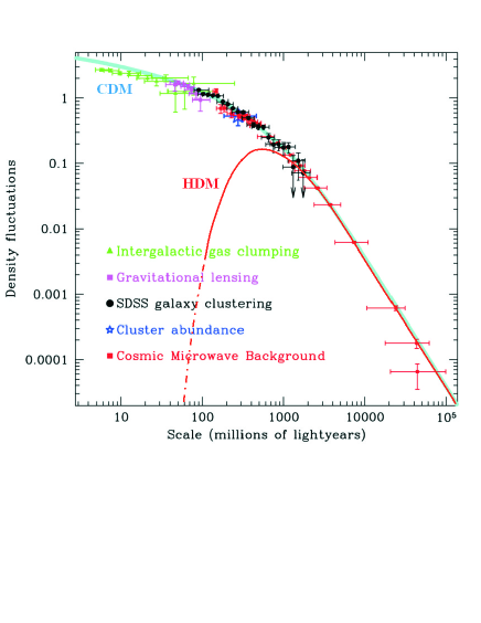
Figure 1: Scale dependence of density fluctuations from CMB anisotropies and large-scale structure. The continuous line labelled by CDM corresponds to a flat model with cold dark matter ($\Omega_{M}=0.28$, $h=0.72$) and a scale invariant spectrum of fluctuations ($n_{s}=1$). The behaviour for $\lambda<\lambda_{eq}\simeq 2.9\cdot 10^{8}$ lightyears is approximately logarithmic, whereas it decays as $\lambda^{-2}$ for $\lambda>\lambda_{eq}$. The line labelled by HDM represents the typical behaviour of a hot dark matter model, with a sharp cut-off for $\lambda<\lambda_{FS}$, (data from SDSS collaboration SDSS )

Another important physical aspect of the cosmological principle is that homogeneity and isotropy are connected to the fact that the present Universe comes from a previous state of thermal equilibrium: the Hot Big Bang. This is a very satisfactory state of affairs because it makes the Universe comprehensible, since its present state can be understood through casual laws without any reference to particular initial conditions. There is however a caveat. As we shall discuss below, the existence of a suitable inflationary phase guarantees that the region of the Universe that is observable today, comes from a tiny patch which was causally connected -therefore able to be in thermal equilibrium- before inflation happened. Thus, it could well be that we live not very near to the edge of a smooth, homogeneous and isotropic patch caused by inflation, with the Universe as whole being chaotic. So, it is possible that the Cosmological Principle is valid only in a local sense.

The Cosmological Principle together with the Equivalence Principle dictates the geometry of the Universe given by the Robertson-Walker metric

$$ds^{2}=-dt^{2}+a^{2}(t)\left(\frac{dr^{2}}{1-kr^{2}}+r^{2}(d\theta^{2}+{\rm sen}^{2}\theta\,d\phi^{2})\right)\,~{}~{}.$$ (2)

In this metric the function $a(t)$ is the scale factor of the Universe, the constant $k=1,0,-1$ specifies the sign of the spatial curvature of the Universe, and $t$ is the cosmic time. The cosmic time is the time measured by the fundamental or comoving observers which are at rest with respect to the expansion. They can be characterized as those measuring zero dipole anisotropy in CMB. Since the peculiar velocity of the Sun is roughly 370 km/s with respect to CMB, the time measured by our watches at Earth coincides with cosmic time with an error of approximately 1 part in $10^{6}$.

The coordinates $r,\theta,\phi$ are (spherical) comoving coordinates meaning that comoving observers remain at rest in these coordinates. Velocities with respect to these coordinate systems are called peculiar velocities. Galaxies are nearly comoving, their peculiar velocities being about a few hundred km/s.

As the Universe expands, physical distances between comoving objects and wavelenghts scale with $a(t)$. Thus, the wavelength of a freely propagating photon is stretched in proportion to the expansion factor from the epoch of emission to detection

$$1+z=\frac{\lambda_{\mathrm{obs}}}{\lambda_{\mathrm{em}}}=\frac{a_{\mathrm{obs}}}{a_{\mathrm{em}}}~{}~{}.$$ (3)

This expression also defines the redshift parameter $z$.

The observable region of the Universe at a given time is limited by the physical distance that light can travel since the Big Bang. This distance, called the particle horizon is directly related to the scale factor by $d_{H}(t)=a(t)\int_{0}^{t}dt^{\prime}a^{-1}(t^{\prime})$.

The Cosmological Principle also restricts the form of the material content of the Universe. Since a perfect fluid can be characterized by its isotropy around observers comoving with the fluid, the stress-energy tensor for the material content of the Universe must have the perfect fluid form

$$T_{\mu\nu}=pg_{\mu\nu}+(p+\rho)u_{\mu}u_{\nu}~{}~{},$$ (4)

where $p$ and $\rho$ are the pressure and the energy density measured by a comoving observer, and $u^{\mu}$ is the four velocity of the fluid.

2.3 FRWL Models

The Robertson-Walker (2) metric provides the kinematical framework for cosmological models. It plays a similar role to the metric of the two-dimensional sphere in the study of Geography. Thus the analysis of cosmological observations based only in the RW metric, without any dynamical assumptions, is sometimes called Cosmography.

Cosmological dynamics i. e.  the study of the time variation of the scale factor and the cosmological densities for the various matter species entering the composition of the Universe, is obtained by the combination of the second basic element of General Relativity: the dynamical equations for the gravitational field, and the Cosmological Principle. This leads to the Friedmann-Lemaître equation

$$H^{2}=\frac{8\pi G}{3}\rho+\frac{1}{3}\Lambda-\frac{k}{a^{2}}~{}~{},$$ (5)

and the energy conservation equation

$$\frac{d}{dt}(\rho a^{3})=-p\frac{d}{dt}a^{3}~{}~{},$$ (6)

where $H=\dot{a}/a$ is called the Hubble parameter. Its present value $H_{0}$ is the Hubble constant, usually expressed in terms of the adimensional number $h$ in the form $H_{0}=100\,h$ km s^-1 Mpc^-1. Thus, solving Friedmann-Lemaître equation (5) relates the expansion rate of the Universe given by the Hubble parameter $H(t)$, with the cosmic time $t$ and the red-shift parameter $z$.

The various species entering the cosmological models are assumed to satisfy linear equations of state of the form $p=w\rho$. This includes in particular the cases of photons in the CMB or an ultrarelativistic plasma $(w=1/3)$, cold non relativistic matter $(w=0)$, and the cosmological constant $(w=-1)$. In addition, the density parameters for each species are defined as $\Omega_{i}=8\pi G\rho_{i}/3H^{2}$, where $3H^{2}/8\pi G$ is the critical density corresponding to a flat Universe $(k=0)$ with $\Lambda=0$. Moreover Friedmann-Lemaître equation (5) when rewritten as

$$\sum_{i}\Omega_{i}+\Omega_{\Lambda}-\frac{k}{a^{2}H^{2}}=1~{}~{},$$ (7)

relates the density parameters to the spatial curvature, including $\Omega_{\Lambda}=\Lambda/3H^{2}$ as the density parameter for the cosmological constant. Thus flat universes are those fulfilling the condition $\sum_{i}\Omega_{i}+\Omega_{\Lambda}=1$. It is important to remark that all universes having a Big Bang, are nearly flat at early times since the density parameter for curvature $\Omega_{k}=-k/a^{2}H^{2}\rightarrow 0$ as $t\rightarrow 0$

On the other hand the temporal evolution for the densities is given, in terms of the red-shift parameter $z$, by the energy conservation equation (6), and the equation of state

$${\Omega_{i}H^{2}(1+z)^{\left(-3-3w_{i}\right)}=\frac{8\pi G}{3}\rho_{i}(1+z)^{\left(-3-3w_{i}\right)}=\mathrm{const.}}$$ (8)

As we shall discuss below, observations favour a present Universe which is nearly flat and composed of cold matter and a cosmological constant, with present values of density parameters $\Omega_{M}\approx 0.27$ and $\Omega_{\Lambda}\approx 0.73$. As shown in Figure 2 the selection of a region in the $\Omega_{M}$-$\Omega_{\Lambda}$ plane centered about these values, arises from the combination of observational information from supernova type Ia Hubble diagrams, CMB anisotropies, and clustering of galaxies in LSS. Taking into account the measured value of the Hubble constant $h\approx 0.72(10\%)$ Hubble and solving Friedmann-Lemaître equation for these models, yields an age for the Universe around 13.7 Gyr, and a distance to the particle horizon about 14-15 Gpc.

According to the evolution equation for the densities (8), $\Omega_{\Lambda}$ decreases and $\Omega_{M}$ increases with increasing red shift. Thus, going backwards in time, for $t\lesssim 1$ Gyr, $\Omega_{\Lambda}$ becomes negligible and we are left with a critical Universe dominated by cold matter, until radiation begins to dominate. In addition, from the analysis of CMB anisotropies, and from BBN, it follows that only about $15\%$ of this cold matter are baryons, the rest being cold dark matter.

Planck’s formula for blackbody radiation translates the present CMB temperature $T=2.725$, into an energy density of CMB photons $\Omega_{\gamma}h^{2}=2.48\times 10^{-5}$. Including three massless (or very light) species of neutrinos, the total energy density in radiation would be at present $\Omega_{R}h^{2}=2.48\times 10^{-5}$, which is negligible in front of the energy density in cold matter. However as we go backwards in time, the number density of radiation particles scales as $a^{-3}$, and the wavelength shrinks in proportion to the scale factor $a$. Therefore, the energy density in radiation scales as $a^{-4}$ while the energy density in cold matter goes with $a^{-3}$. As a consequence, at sufficient earlier times, radiation dominates the energy density of the Universe. For $h\approx 0.72$ and $\Omega_{M}\approx 0.27$ the energy densities in matter and radiation become equal at $z_{\mathrm{eq}}\approx 3300$, which corresponds to an approximately 55 kyr old Universe.

3 Hubble Law, Hubble Diagrams and Dark Energy

In the approximation in which galaxies are comoving, the physical distance to a given galaxy scales with $a(t)$, and consequently its recession velocity $V$ is related to its physical distance $d$ at a given time, by

$$V=Hd~{}~{}.$$ (9)

This is the theoretical Hubble law which is exact, and a direct consequence of the Robertson-Walker form of the cosmic metric. This relation cannot be directly checked because neither the recession velocities nor the physical emission distances to galaxies are empirically measurable.

The Robertson-Walker form of the metric was stablished in 1936. Earlier, in 1929 E. Hubble found the empirical Hubble law

$$z=H_{0}d_{\mathrm{L}}~{}~{},$$ (10)

linearly relating the red-shift of galaxies to their luminosity distance. The luminosity distance is defined as $d_{\mathrm{L}}=\sqrt{L/4\pi\mathcal{F}}$, where $L$ is the absolute luminosity of the source and $\mathcal{F}$ its apparent luminosity, i. e. the flux of energy received in the collecting surface of the telescope. So, luminosity distance $d_{\mathrm{L}}$ is defined as such that a source of absolute luminosity $L$, located in a static Euclidean space, would produce a flux $\mathcal{F}$ at distance $d_{\mathrm{L}}$. From RW metric, it follows that the relation between $d_{L}$ and the red-shift parameter $z$ is nonlinear. To second order this relation takes the form

$$H_{0}\,d_{\mathrm{L}}(z)=z+\frac{1}{2}(1-q_{0})z^{2}+\cdots~{}~{},$$ (11)

where $q=-a\ddot{a}/\dot{a}^{2}$ is the deceleration parameter of the Universe and $q_{0}$ its present value. It follows then from RW metric, i. e. from Cosmological Principle, that the empirical Hubble law can be expected to be true only for $z\ll 1$. On the other hand for $z\ll 1$, the approximate equalities $d\approx d_{\mathrm{L}}(z)$ and $V\approx z$ hold. Thus empirical and theoretical Hubble laws coincide in this regime. In this weak sense checking Hubble’s law is also a check of the RW metric.

To accurately check Hubble’s law, measuring $H_{0}$ within the linear approximation to (11), and eventually going deeper in red-shift to determine $q_{0}$, has been a central research program in Cosmology since 1929, called Hubble program. The key observational tool for this endeavour are standard candles: luminous sources whose absolute luminosity has been properly calibrated. Once a class of sources has been calibrated, a Hubble diagram can be obtained by representing these sources in a two-dimensional plot of luminosity distances versus red-shifts, the final goal being to extract from the observational points the cosmological parameters $H_{0}$ and $q_{0}$. This program received a major boost with the launching of the Hubble Space Telescope (HST) in 1990, whose so-called Key project was to perform a precise measure of $H_{0}$.

Measuring cosmic distances starts by the trigonometric parallax of nearby stars, due to the annual motion of the Earth around the Sun. From this starting point, a cosmic distance ladder is built by means of standard candles. This method works typically by finding precise correlations between the absolute luminosity and another observable for a definite class of objects. The first and basic step is provided by Cepheid variable stars, whose absolute luminosity is tightly related to its period. HST has been able to resolve thousands of Cepheid variables in galaxies up to 20 Mpc. Once the distances to these nearby galaxies are fixed, five different methods are used to go up to 400 Mpc. Three of them are based on global properties of spiral and elliptical galaxies: Tully-Fisher relation that links rotation velocities of spiral galaxies to their luminosity, relation between star velocities dispersion and luminosity in ellipticals, and fluctuations in galaxies surface brightness. The other two are based on the use of supernovae type Ia (SNe Ia), and supernovae type II (SNe II) as standard candles. The combination of all these methods yields for the Hubble constant a weighted average $H_{0}=72\pm 8$ km s^-1 Mpc^-1 Hubble . It is most remarkable that this value for $H_{0}$ agrees with the value obtained by the analysis of the CMB anisotropy map provided by WMAP: $H_{0}=71$ km s^-1 Mpc^-1 $(5\%)$.

Due to their big absolute luminosity, SNe Ia are the most far reaching standard candles in red-shift. This makes these objects ideal tools to investigate the deceleration parameter $q_{0}$. In 1998 two groups: the High z Supernovae Search Team (HZT) and the Supernova Cosmology Project (SCP) using SNe Ia, reported the discovery of the accelerated expansion of the Universe ($q_{0}<0$) SN . The result appears through an exceeding faintness of supernovae as they would have in a decelerating universe. Notice that from eq. (11), an accelerating universe ($q_{0}<0$) results in bigger luninosity distances -hence, fainter objects- for the same red-shift than a decelerating one ($q_{0}>0$). Thus, once other astrophysical effects like dust or evolutionary effects have been discarded, the exceeding faintness of supernovae should be interpreted as due to the acceleration of the Universe expansion.

Friedmann’s equations (5), (6) imply that an accelerating Universe should contain part of its energy density in a substance with equation of state parameter $w<-1/3$. This kind of substance goes under the name of dark energy, and the most obvious candidate is a cosmological constant ($w=-1$). For a model composed of dark matter plus a cosmological constant, the deceleration parameter $q=\frac{1}{2}\,\Omega_{M}-\Omega_{\Lambda}$, and as shown in Figure 2, the supernovae data select a linearly shaped maximum likelihood region in the $\Omega_{M}-\Omega_{\Lambda}$ plane. So, supernovae data alone, suffice to stablish the acceleration of the Universe with a very high confidence level. When supplemented with the data coming from CMB and LSS, a best fit is obtained for $\Omega_{M}\approx 0.28$ and $\Omega_{\Lambda}\approx 0.72$, corresponding to a nearly flat Universe.

Although the LSS models favored the so-called $\Lambda$CDM (cosmological constant plus cold dark matter) scenario, the discovery of the acceleration of the Universe in 1998 came as a surprise, since a universe filled with cold matter ($w=0$) decelerates ($q=\frac{1}{2}\,\Omega_{M}>0$). However as explained above, when we go backwards in time, $\Omega_{M}$ grows and $\Omega_{\Lambda}$ decreases. So, at earlier times there should have been a decelerating period of the Universe. In fact, very recently vuelta , using the HST, 16 new type Ia supernovae has been found at very high red-shift, up to $z\approx 1.7$, which give conclusive evidence for this decelerating period. These newly discovered SNe Ia, together with the 170 previously reported confirm the concordance model with $\Omega_{M}\approx 0.28$ and $\Omega_{\Lambda}\approx 0.72$, and give a value for the red-shift of the transition between the accelerating and deccelerating epochs $z=0.46\pm 0.13$. It is the most remarkable that the confirmation of the effect of deceleration in supernovae, almost fully rule out alternative astrophysical explanations like dust or evolutionary effects for the luminosity distance versus red-shift distribution, since it is very unlikely for these effects to exactly mimick the deceleration/acceleration transition.

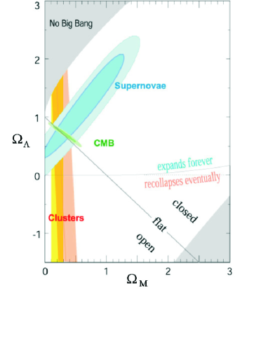
Figure 2: Matter density $\Omega_{M}$ vs. vacuum energy density $\Omega_{\Lambda}$ 68$\%$ and 95$\%$ C.L. contours for supernovae, cluster and CMB data, (from Supernova/Acceleration Probe: SNAP collaboration SNAP )

In addition to the cosmological constant, other forms of dark energy could be possible with a different or even a variable equation of state $w$. An interesting class of models are quintessence models in which dark energy is the energy density of an evolving scalar field, much the same way as the inflaton during the inflationary phase of the Universe. For a constant equation of state, SNe Ia data yield $w=-1.02_{0.19}^{0.13}$ and $w<-0.76$ to 95% confidence level vuelta . An alternative proposal to dark energy as an explanation for the deceleration/acceleration of the Universe could be the weakening of gravity in our 3+1 dimensions by leaking into the extra dimensions as suggested by string theories. A major observational effort will be needed to discriminate among these competing models.

4 Large Scale Structure and Dark Matter

Far from a smooth distribution, matter exhibits a complex clustering pattern in the Universe. Thus, there are regions in which matter is strongly clumped forming galaxies, clusters and even larger structures, whereas at the same time, we can also find almost empty regions with very low densities. In fact, strong inhomogeneities can be found at galactic scales ($\sim$ 10 kpc), where the density contrast can be as large as $\delta\rho/\rho\sim 10^{2}$. Galaxies, which can be considered as the elementary building blocks of structures, are not homogeneously distributed either, but grouped hierarchically into groups, clusters and superclusters, the latter ones extending over distances of tens of Mpc. Filament-like chains of galaxies connect different superclusters in a network with scales of around 100 Mpc. Most of the matter distributes on the walls of this cell-like structure with large voids in between. In Figure 1 we can see a data plot showing the scale dependence of the density contrast. Each point represents the density fluctuation measured at a given scale $\lambda$, which is obtained by comparing the avarage density within a sphere of radius $\lambda$, as it is placed at different spatial positions. As we see from the data, the density contrast declines as we take larger and larger spheres, in agreement with the Cosmological Principle. Thus, we can conclude that the Universe can be considered as approximately homogeneous only on very large scales ($\sim$ 1000 Mpc).

The SCM allows us to understand the growth of these structures from seeds of primordial density fluctuations. However, the origin of such seeds is left unspecified, this being one of the most important limitations of the classical standard cosmology. In Section 7 we will see a possible generation mechanism based on the idea of inflation. Leaving aside the issue of the origin, the growth mainly takes place during the matter dominated era as more and more matter is attracted towards the initially overdense regions. When the structure is sufficiently large (larger than the so-called Jeans scale), its gravitational self-attraction is able to decouple it from the Hubble expansion, forming a bound object. For small density fluctuations (linear regime), the growth rate is linear with the scale factor. This means that the total growth from the matter-radiation decoupling time ($a_{dec}\sim 10^{-3}$) until present ($a_{0}=1$) would be a factor $10^{3}$. However, the amplitude of CMB fluctuations at that time, measured by the COsmic Background Explorer (COBE) satellite, was only $\delta\rho/\rho\sim\delta T/T\sim 10^{-5}$. This obviously poses a problem since fluctuations have not had enough time to reach the non-linear regime $\delta\rho/\rho\gg 1$. Notice that in the previous reasoning it is assumed that matter fluctuations are comparable to temperature fluctuations at decoupling. This is indeed the case for baryons, which were coupled to photons until decoupling time, and implies that a universe dominated by baryons at the time of decoupling is not consistent with galaxy formation.

However, if there existed a new type of weakly coupled matter, which did not interact with radiation, its density fluctuations could have started growing much before, thus explaining the apparent mismatch. This is one of the strongest arguments in favor of the existence of dark matter. Once, baryons and radiation decouple, baryons will fall in the potential wells created by dark matter, their density fluctuations acquiring the same amplitude as that of dark matter.

The nature of dark matter determines the final density distribution at different scales. At present there are important projects which aim to collect information about the distribution of galaxies in the Universe. They are galaxy redshifts catalogues such as the 2dFGRS 2df and the SDSS SDSS . The first one, which has been completed recently, has measured the redshift of 221000 galaxies over a five years period. The SDSS is in progress and is expected to measure the position and the absolute brightness of 100 million celestial objects. The information obtained from these catalogues combined with that coming from CMB anisotropies and high-redshift supernovae observations is allowing us to determine the cosmological parameters with unprecedented accuracy (see Fig. 2), and to shed light on the nature of dark matter.

Let us see how dark matter affects structure formation. For that puropse it is convenient to differentiate between the so-called hot (HDM) and cold dark matter (CDM) scenarios. In the hot case, dark matter is made out of light particles, which were still ultrarelativistic at the beginning of the structure formation period, with the typical candidate being a light neutrino. Since hot dark matter particles propagate close to the speed of light, they can escape from overdense regions into underdense ones, erasing the density fluctuations on scales smaller than the free-streaming scale $\lambda_{FS}$. This is the maximum distance that a particle can travel from the initial time until matter-radiation equality. Typical values are $\lambda_{FS}\sim 40$ Mpc, corresponding to the size of a large cluster, for a neutrino (or any other light particle) mass around $m_{\nu}\sim 30$ eV. This means that, in this scenario, galaxies cannot grow directly from primordial fluctuations. Superclusters should form first, reach the non-linear regime and then, by fragmentation, give rise to small clusters and galaxies. As a consequence the power spectrum of density fluctuations should be strongly peaked around the $\lambda_{FS}$ scale (see Fig. 1). However, recent CMB data together with 2dFGRS or SDSS information on the matter power spectrum, constrain the above effect. The results show that hot dark matter cannot be the dominant dark matter component and $\Omega_{\nu}h^{2}\leq 0.0076$ (2dF+WMAP at 95 $\%$ C.L.). This bound can be translated into a very strict limit on the sum of the neutrino masses $\Sigma_{i}\;m_{\nu_{i}}\leq 0.71$ eV, which improves by several orders of magnitude the laboratory limits.

In the cold dark matter case, dark matter particles are already non-relativistic at matter-radiation equality. Thus, free-streaming damping is not a problem. As shown in Fig. 1, an enormous variety of observations at very large scales ($\mathrel{\mathop{\kern 0.0pt\hbox to0.0pt{\raise 0.86108pt\hbox{$>$}\hss}}\lower 3.87495pt\hbox{\kern-1.90002pt$\sim$}}1$ Mpc), from cosmic microwave background anisotropies, galaxy surveys, cluster abundances or Ly-$\alpha$ forest are successfully explained within the CDM framework. Despite its success at large scales, the model exhibits certain difficulties at sub-galactic scales. In particular, high resolution N-body simulations of dark halos show cuspy density profiles which contradict observations from low surface brightness galaxies and dwarfs which indicate flatter density profiles. In addition, CDM also predicts too many small subhalos within simulated larger systems, in contradiction with observations of the number of satellite galaxies in the Local Group. In any case a spatially flat Universe with cosmological constant and cold dark matter ($\Lambda$CDM) is generally accepted at present as the Standard Model in Cosmology.

4.1 Nature of Dark Matter

Apart from the difficulties of a baryon dominated universe to explain galaxy formation, there are additional evidences that the luminous mass of the Universe is only a small fraction of the total matter density DM . This deficit is present in two different contexts: first at galactic scales, where dark matter is believed to form spherical halos several times bigger than the galactic disks; and second at cosmological scales. Many different kinds of observations such as rotation curves of galaxies, weak gravitational lensing, cluster abundance, virial motions in clusters, matter power spectrum, CMB anisotropies, …, agree in a value for the total matter $\Omega_{M}=0.27\pm 0.04$. This value should be compared to the baryon density $\Omega_{B}=0.044\pm 0.004$ and to the luminous mass density $\Omega_{lum}=0.006\pm 0.003$, i.e we find $\Omega_{lum}<\Omega_{B}<\Omega_{M}$. We thus have two dark matter problems, namely, there are missing baryons which do not contribute to the luminous matter and there is non-baryonic dark matter which make up most of the matter of the Universe.

Concerning the baryonic dark matter problem, it is difficult to find dark baryons in the galactic halos. They could be present in the form of hot or cold clouds of hydrogen, although an entire halo made of gas would conflict with observations of absortion or emission of radiation. They could form massive compact halo objects (MACHOs) similar to big planets. However the current limits from EROS and MACHO microlensing observations show that less than 25$\%$ of standard halos can be composed of MACHOs with masses between $10^{-7}-1$ M_⊙.

On the other hand, the nature of non-baryonic dark matter is even a greater mistery. Different possible explanations include: massive neutrinos, modifications of gravity at large distances or the existence of a background of new weakly interacting massive particles (WIMPs). A natural dark matter particle should be neutral, stable, massive and weakly interacting, so that its relic density could contribute in an important way to the matter density. Accordingly a massive neutrino would be the most economical solution. However, different limits prevent neutrinos from being a viable candidate. Thus, apart from the strong limit coming from 2dF + WMAP mentioned above, simply imposing that relic neutrinos do not overclose the Universe, i.e. $\Omega_{\nu}\mathrel{\mathop{\kern 0.0pt\hbox to0.0pt{\raise 0.86108pt\hbox{$<$}\hss}}\lower 3.87495pt\hbox{\kern-1.90002pt$\sim$}}0.3$, then their masses should be either smaller than $\sim 20$ eV or larger than $\sim 20$ GeV.

Let us study in more detail each possibility. In the case of light (hot) neutrinos, if they are required to make up the galactic halos, their mass density should be $\rho_{halo}\simeq 0.3$ GeV cm^-3. However, their number density cannot exceed the limit imposed by the Pauli exclusion principle, so that their masses should be sufficiently high. In particular we get $m_{\nu}\mathrel{\mathop{\kern 0.0pt\hbox to0.0pt{\raise 0.86108pt\hbox{$>$}\hss}}\lower 3.87495pt\hbox{\kern-1.90002pt$\sim$}}20$ eV for spiral galaxies and $m_{\nu}\mathrel{\mathop{\kern 0.0pt\hbox to0.0pt{\raise 0.86108pt\hbox{$>$}\hss}}\lower 3.87495pt\hbox{\kern-1.90002pt$\sim$}}100$ eV for dwarf galaxies (Tremaine-Gunn limit), in contradiction with the overclose limit. In the case of heavy (cold) neutrinos, the overclose limit is much larger than the laboratory limits on the three known neutrino species, but still there is the possibility of the existence of a stable heavy fourth generation of Dirac or Majorana neutrinos. Current direct detection experiments have enough sensitivity to detect halo particles with cross-sections typical of weak interactions and masses above 20 GeV. However, at present there is no compelling evidence of the detection of such particles, so that a fourth generation of neutrinos is excluded. (DAMA experiment claims the detection of an annual modulation in its dark matter signal. However, such a result seems to be incompatible with other direct detection experiments as CDMS).

The absence of cold dark matter candidates within the known particles is one of the most pressing arguments for the existence of new physics beyond the Standard Model, either as new particles or as modifications of the gravitational interaction at large distances. Among the proposed new particle candidates, we find, on one hand, the axion which is the Goldstone boson associated to the spontaneous breaking of the Peccei-Quinn symmetry postulated to solve the strong CP problem of QCD. The production of axions in the early Universe mainly takes place through the so-called misalignment mechanism in which the $\Theta$ angle is initially displaced from its equilibrium value $\Theta=0$, and oscillates coherently. Such oscillations can be intrepreted as a zero-momentum Bose-Einstein condensate which essentially behaves as a non-relativistic matter fluid. Despite the fact that axions are light particles, this non-thermal mechanism produces cosmologically important energy densities. On the other hand we have the thermal relics, produced by the well-known freeze-out mechanism in an expanding Universe. They are typically weakly interacting massive particles (WIMPs) such as the neutralino in supersymmetric theories (for a recent review see DM ). In addition to their weak interactions with ordinary particles included in the EPSM, these candidates usually have also very weak self-interactions (collisionless).

At present there are several kinds of experiments (ground based and satellite borne) which aim to detect cold dark matter halo particles, either directly or indirectly. Direct detection experiments are based on the possibility of measuring the recoil energy that a target nucleus acquires in the elastic collision with a DM particle. Some of the experiments in progress are: DAMA, CRESST and GENIUS, at Gran Sasso Laboratory or CDMS at Soudan mine. The indirect experiments are based on the possibility of detecting the annihilation products of halo DM particles. Typically they include: gamma ray telescopes such as MAGIC (ground based) or GLAST (satellite) which could be sensitive to annihilations into pairs of photons; antimatter detectors such as AMS which can detect positrons produced in $e^{+}e^{-}$ annihilations; and finally high-energy neutrino telescopes such as ANTARES or AMANDA which will be sensitive to neutrino-antineutrino annihilations. The projected sensitivity of these experiments covers a part of the parameter regions (masses and interaction cross-sections) which will be explored by future particle accelerators such as LHC or Tevatron II. However their relative low cost make them very promising alternatives for finding new physics.

5 The Cosmic Microwave Background

The existence of a Cosmic Microwave Background with present temperature around 5K, was theoretically predicted in 1948 by G. Gamow, R. Alpher and R. Hermann, as a necessary relic of a hot phase of the Universe in which the light elements should have been cooked through nuclear reactions starting with primordial protons. This work largely ignored during almost two decades, can be regarded with hindsight as the foundational paper of the Hot Big Bang model. On the other hand, in year 1964, A. Penzias and W. Wilson who where working at Bell Telephone Laboratories to fit an antenna for satellite communications operating in the microwave range, found to his annoyance an “excess” radio noise isotropically distributed and corresponding to a temperature of about 3K, whose origin they did not know and did not hypothesized about. In the same year the group of theoreticians of Princeton University: B. Dicke, P. Peebles, P. Roll, and D. Wilkinson, who did not know or had forgotten about the work of Gamow et al, where following a similar line of reasoning. In fact they where thinking about building a radiometer to detect the fossil radiation left out from a primitive dense and hot phase of the Universe, when they knew about Penzias and Wilson observations and correctly interpreted them as the cosmic background radiation they were looking for. Similar considerations were also done by Y. Zeldovich and his group in Moscow around the same time. Thus CMB was accidentally discovered in 1964, and Penzias and Wilson (but not Gamow et al. nor Dicke et al.) were awarded the Nobel prize in 1978.

Since the temperature of the photons in CMB scales according to $T\propto a^{-1}$, the existence of CMB together with the expansion of the Universe imply a hot early phase, which becomes hotter and denser as we go backwards in time. In this primitive epoch, the Universe is a plasma containing more and more species of particles as we go backwards in time and new channels are opened for pair production to the increasingly energetic photons. In this way, when the photons are cold enough, $T\sim 3000$ K, the baryons and electrons recombine to form neutral hydrogen and helium atoms, and the photons are free to propagate: the Universe becomes transparent. This happens for a red-shift parameter $z_{\mathrm{rec}}\sim 1100$, which corresponds to an age of about 380 Kyr. The recombination red-shift $z_{\mathrm{rec}}$ defines a last scattering surface for charged particles and photons, or cosmic photosphere, where CMB is coming from. Indeed, this is not a mathematical surface but it has a thickness which can be modeled by a Gaussian visibility function with a width $\delta z\simeq 80$.

CMB radiation is therefore a relic from $z_{\mathrm{rec}}\sim 1100$, beyond which the Universe is optically thick in almost all wave bands, and it carries vital information about the processes and features of the early Universe CMB . So, since its discovery and specially in the last fifteen years there has been an intense observational effort on CMB. The COBE satellite launched in November 1989 made a major breakthrough. With the FIRAS (far infrared absolute spectrophotometer) instrument on board, it was stablished the almost perfect blackbody spectrum of CMB, which witnesses the perfect thermal equilibrium state from which our Universe is coming from. It is most remarkable that such a pure blackbody spectrum has never been observed in laboratory experiments. In addition, with the help of the DMR (differential microwave radiometer) instrument, a map of CMB temperature anisotropies was obtained for the first time. After COBE a series of ground and balloon based measurements: ARCHEOPS, BOOMERANG, DASI, MAXIMA, VSA and for smaller scales CBI and ACBAR, have been carried out to improve the quality of temperature anisotropies distribution data. The most important recent advance has been the fisrt year of operation results from NASA’s WMAP (Wilkinson Microwave Anisotropy Probe) CMB ; WMAP . Launched in June 2001, the first data release in February 2003, corresponds to a twofold full coverage of the sky and provides a much more precise anisotropies map than COBE’s (see Fig. 3). WMAP is funded to operate for at least another three years, completing and eightfold covering of the sky and increasing statistical accuracy. After that, ESA’s satellite Planck Planck , scheduled for launch in 2007, will take over. As WMAP, Planck will be stationed at Lagrange L2 point of the Sun-Earth system, and will cover the full sky reaching an angular resolution up to one tenth of degree.

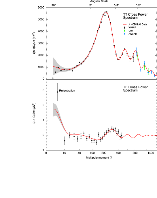
Figure 3: TT and TE angular power spectra from WMAP one-year data, CMB

The CMB temperature distribution in the sky, being a function defined on a sphere is most naturally analyzed through an spherical harmonics expansion

$$T(\theta,\phi)=\sum_{\ell m}a_{\ell m}Y_{\ell m}(\theta,\phi)$$ (12)

The monopole component gives the mean temperature of CMB $T=2.725\pm 0.001$ K, which according to Planck’s law for blackbody radiation, corresponds to a photon number density $n_{\gamma}=411$ cm^-3, and an energy density $\rho_{\gamma}=0.260$ eV cm^-3. The largest anisotropy is the $\ell=1$ dipole term with amplitude $3.346\pm 0.017$ mK interpreted as the result of the Doppler shift caused by the Solar system motion relative to the CMB. The implied velocity for the Sun is $v=368\pm 2$ km s^-1, directed towards Hydra-Centaurus (more precisely, right ascension $=166\pm 3$ and declination $=-27.1\pm 3)$. This interpretation is reinforced by the yearly modulation of the anisotropy due to Earth’s motion around the Sun, and also by measurements of the velocity field of local galaxies. This rather impressive finding about what could be called “our home’s absolute velocity” embodies a delicious irony: the negative result of the Michelson-Morley experiment in 1887 in detecting Earth’s motion with respect to aether (the hypothetical mechanical medium supporting the propagation of light), motivated the introduction of Special Relativity. On these foundations General Relativity was built and Cosmology developed during the XXth century. Finally, towards the end of the last century, the peculiar velocity of the Earth was measured with light (CMB) playing the role of aether, and without contradicting Relativity. Simply, CMB photons materialize a convenient comoving coordinate system.

Once the monopole and the dipole have been removed from the expansion (12), we are left with the CMB intrinsic anisotropies which are of the order of, or below $10^{-5}$ in all angular scales, and contain the imprints of the early Universe physics at radiation-matter decoupling. Most of the cosmological information is contained in the two point temperature-temperature (TT) correlation function. This quantity is defined by averaging the product of the fractional temperature deviations in directions $\vec{n}$ and $\vec{n^{\prime}}$ over the sky, and expanding the result in Legendre polynomials

$$C(\theta)\equiv\langle\,\frac{\Delta T(\vec{n})}{T}\frac{\Delta T(\vec{n^{\prime}})}{T}\,\rangle=\sum_{\ell=0}^{\infty}\frac{2\ell+1}{4\pi}C_{l}P_{l}(\cos\theta)$$ (13)

The expansion coefficients $C_{l}$, when represented as function of $\ell$ (more suitably $\log\ell)$ give the so-called angular power spectrum which is the key function in comparing theory and observations. The cosmological parameters affect the form of this function and this is the way in which they can be deduced from CMB observations. Several physical mechanisms contribute to the angular power spectrum at different angular scales $\theta\sim\pi/\ell$. An important milestone is the size of the comoving Hubble radius at decoupling. This is half the size of the comoving particle horizon at that time if inflation had not happened before, and far from covering the whole sky, it subtends an angular opening $\theta\sim 0.86\sqrt{\Omega}$, with $\Omega$ being the present total density parameter of the Universe. This is the origin of the horizon problem that inflation solves as we will discuss below.

The description of the physics contained in $C_{l}$, can be separated into three main regions. i) The Sachs-Wolfe plateau for $\ell\leq 100$: This region corresponds to angular scales bigger than the Hubble radius at decoupling and it is dominated by the so-called Sachs-Wolfe effect: the photons coming from denser regions have to climb out of deeper gravitational potential wells and become redder. A nearly scale invariant spectrum of density perturbations, as predicted by inflation, agrees with a plateau for this effect. Also, the integrated Sachs-Wolfe effect due to the time variation of the gravitational potential along CMB photons world lines, and gravity waves too, are expected to contribute in this large angular scale region, although these effects are buried in the cosmic variance. This means that doing an statistical analysis of fluctuations for a given set of cosmological parameters, but having only one realization of these fluctuations (our Universe) forces to introduce a kind of ergodic hypothesis: averages of patterns over parts of the sky, extended to the full sky by periodicity, would be equal to averages over different full sky realizations of perturbations for the same set of parameters. Indeed this method becomes increasingly uncertain at large angular scales and this is the meaning of the term cosmic variance.

ii) The acoustic peaks for $100\leq\ell\leq 1000$. Before decoupling, photons, electrons and baryons form a tightly coupled fluid with the photons providing the pressure and the baryons the inertia. The fluid supports acoustic waves whose fundamental halfperiod is determined by the Hubble length at decoupling, and in turn its wavelength is obtained from the known value of the sound speed in the plasma. In this oscillating plasma denser regions correspond also to hotter regions (notice the opposite sign of this effect as compared to Sachs-Wolfe) according to Planck’s law. Therefore a series of peaks in $C_{l}$ are expected. The first one corresponding to the fundamental acoustic mode, and subsequent ones for higher harmonics. These peaks were theoretically predicted by P. Peebles, and Y. Zeldovich and collaborators already in 1970, and the empirical proof of their existence is a major success of modern cosmology. The position and height of the acoustic peaks encode information about the cosmological parameters. Indeed the angular scale subtended today by the fundamental acoustic wavelength depends on the underlying geometry. This is how the position of the first peak, stablished by WMAP to be around $\ell\sim 220$, results in a flat Universe with $\Omega=1.02\pm 0.02$. This way of stablishing the flatness of our Universe is in fact very similar in essence to the method attributed to Gauss, who supposedly measured the three angles formed by three peaks in the Harz mountains, in order to check space geometry. In this case the triangle is the one formed by the acoustic fundamental halfwavelenght sitting on the last scattering surface, and two lines of sight from its extremes to us. Thus in a $\Lambda$CDM model, the position of the first acoustic peak determines $\Omega_{M}+\Omega_{\Lambda}$, while the difference $\Omega_{M}-\Omega_{\Lambda}$ can be extracted from SNe Ia Hubble diagrams as explained above. The second peak is not as high as the first one because the baryons feel the radiation pressure but cold dark matter does not, and as a consequence the relative height of the first and second peak gives the amount of baryons in the Universe. Combined results from WMAP, CBI and ACBAR yield $\Omega_{B}h^{2}=0.023\pm 0.001$. In turn this result, together with the photon number density, fixes a very important cosmic number, namely the baryon/photon ratio or specific entropy of the Universe, only from CMB data. The resulting value is $\eta_{10}\equiv 10^{10}\eta=6.14\pm 0.25$. It is very remarkable, and a strong indication of the maturity of the SCM that this value is consistent with the determination of $\eta$ via the physics of BBN when the Universe was three minutes old. In addition, the relative height of the first three peaks provides a determination of $\Omega_{M}$. The Hubble parameter $H_{0}$ can be also extracted from the angular power spectrum, although the dependence of its shape with respect to $H_{0}$ is more involved. WMAP gives $h=0.71(5\%)$, also in good agreement with Hubble diagrams.

iii) The damping tail for $\ell\geq 1000$. As stated above the transition to transparence is not instantaneous and the last scattering surface has a thickness. This leads to the so-called Silk damping of the anisotropies for angular scales smaller than this thickness. In addition, gravitational lensing by non-linear structures at low red-shift, like clusters of galaxies, also deform and smooth the primordial angular spectrum at small scales. As a consequence there are not much primordial anisotropies to observe below 5’ of arc.

Electron-photon Thomson scattering at the last scattering surface transforms anisotropies into CMB photons polarization. The analysis of polarization leads to four new non-vanishing two sky points correlators, with their corresponding angular spectra. The theoretical and observational analysis of these spectra lies at the present frontier of CMB research. For example, Planck satellite is expected to do a significant advance in this respect. In particular the gravity wave contribution to CMB anisotropies could be observed. If the gravity wave perturbations were produced by inflation, these observations would determine the energy scale at which inflation happened. Also the WMAP results concerning polarization measurements have recently uncovered an earlier than expected reionization of the Universe at red-shift $z$ around 20 (see the TE power spectrum in Figure 3). This means that the first stars in the Universe were formed as early as a few hundred million years after Big Bang. Such an early star formation could be challenging for the theory of inflation.

6 Big Bang Nucleosynthesis

While the CMB map of anisotropies can be considered as a photograph of the Universe when it was 380 kyr old, the observed abundances of the light nuclides ¹H, ²D, ³He, ⁴He, and ⁷Li represent the most ancient archaelogical document about the history of the Universe BBN . These light elements were cooked in nuclear reactions when the Universe was about 3 minutes old. The remaining elements is the work of the stars with a little help of cosmic rays spallation. The first to propose a Big Bang nucleosynthesis was G. Gamow in 1946. In fact, a glance at the helium abundance: 24% in weight against 76% for hydrogen, tells us that so much helium can not have been produced by stars. For example, assuming that the age of the Milky Way is $10^{10}$ yr and that it has been radiating all the time at its current power $L_{\mathrm{MW}}=4\times 10^{36}$ W, with all this power coming from the burning of hydrogen into helium, this will account only for less than 1% helium abundance.

The very early Universe is a too hostile environment for nuclei. When the temperature stays above a few MeV -the typical nucleon binding energy- the photons will immediately destroy any existing nuclei. So, nucleosynthesis has to wait until the Universe has cooled down enough. How much is enough? The first step for nucleosynthesis is the formation of deuterium through the reaction $n+p\rightarrow d+\gamma$, and the binding energy of deuterium is 2.22 MeV. However until the temperature does not reach below $0.1$ MeV, formation of deuterium is not possible due to the high specific entropy of the Universe. Put in other words: since the photons outnumber the baryons by a factor $10^{9}$, even well below the binding energy of deuterium, there are enough hard photons in the high energy tail of the Planck distribution to destroy the deuterons as fast as they are produced. Once the deuterons are able to survive they almost instantaneously transform into helium through the reaction $d+d\rightarrow^{4}$He $+\gamma$ and through other fusion reactions involving ³H and ³He as intermediate steps. Production of helium is very much favoured by its comparatively high binding energy $28.3$ MeV. So, from energetic considerations only, it could have happened earlier, but it has to wait until deuterium is formed. This effect is called the deuterium bottleneck. Finally some ⁷Li seven is also formed in collisions of ⁴He with ³He and ³H nuclei. Why not higher nuclei? The reason is that there are not stable nuclei with $A=5$ and $A=8$, and only minute quantities of the nuclei with $A=2,3$ are formed in the synthesis of helium. In addition, the Universe is cooling down very fast, and Coulomb barriers which are higher for higher nuclei suppress nuclear reactions. Therefore BBN stops at this point. So, how do the stars manage to form the rest of the elements like $C$, $N$, $O$, which we the observers are made of? The answer was given by F. Hoyle. There exists a metastable resonance of two ⁴He nuclei. Then, if a third ⁴He nucleus meets the resonance, a ¹²C nucleus is formed by a two steps chain of two particle collisions. This is possible if the temperature and the density are both very high, but in the early Universe, the density and temperature continually drop, and by the time helium has been synthesized, it is too late for this way of producing carbon. However in the interior of stars temperature and density steadily rise as the star evolves, and eventually, the physical conditions for the transformation of helium into carbon -and then into heavier elements- are attained.

The nuclear and elementary particle physics needed to study BBN is well known, and the temporal dependence of the density and temperature can be derived from Friedmann equations. Therefore, the light elements cosmic abundances can be theoretically calculated and compared to the observed ones. The synthesis of light elements is sensitive to physical conditions for temperatures $T\lesssim 1$ MeV, corresponding to an age $t\gtrsim 1$s. Above this temperature neutrons and protons are in thermal equilibrium through weak reactions like $e^{-}+p\leftrightarrow\nu_{e}+n$ and $\bar{\nu_{e}}+p\leftrightarrow e^{+}+n$, and also similar ones for the other neutrino and lepton families. Thus the neutron abundance of protons and neutrons is fixed by the Boltzmann factor $e^{-Q/T}$, where $Q=1.293$ MeV is the neutron-proton mass difference. Thus, as long as thermal equilibrium is mantained, the Universe is running out of neutrons very fast as it cools down. Indeed, if thermal equilibrium held until the deuterium bottleneck is surpassed, very few neutrons would survive. However this is not so because before that, weak interactions “freeze-out” and neutrinos go out of thermal equilibrium. This happens because weak interaction cross sections scale with temperature as $T^{2}$ and non-relativistic particle densities as $T^{3}$, while Hubble parameter $H$ scales as $T^{2}$. Therefore the weak reaction rates $\Gamma_{w}$ over the expansion rate $H$ scale as $\Gamma_{w}/H\propto T^{3}$. Thus, eventually at some temperature, which detailed calculations show to be $T\simeq 1$ MeV, the neutron-proton interconversion go out of thermal equilibrium. At this point, the neutron to proton ratio is about 1/6. From this point on, occasional weak interactions with the tails of the lepton and nucleon Fermi distributions, and neutron beta decay still lower (although much more slowly) the neutron to proton ratio. When the deuterium bottleneck is surpassed at $T=0.1$ MeV, the Universe is about 2 min old, and the neutron to proton ratio has fallen down to $\simeq 1/7$. Therefore, since practically all deuterium transforms into helium, the helium abundance today should be about 25% in weight.

The observed cosmological abundance for primordial ⁴He are in the range 23-24%, in good agreement with the theoretical calculation based in BBN. The observed primordial abundances for deuterium and ⁷Li can de estimated to be in the ranges $D/H=1-7\times 10^{-5}$, and ⁷Li$/H=0.59-4.1\times 10^{-10}$, while for ³He there is not a good estimation, which renders ³He unsuitable as a cosmological probe. In BBN, the light elements abundances depend on the balance between the expansion rate $H$ of the Universe during nucleosynthesis, and the nuclear reactions rates, which in turn depend on the baryon density. All light elements abundances can be explained with a baryon density given by a baryon to photon ratio $\eta_{10}$ in the range 3.4-6.9 (95% CL). This value agrees remarkably well with the value for the same parameter obtained from CBM acoustic peaks, and provides another key confirmation of the BBN theory and of the SCM.

Since the reactions building ⁴He are so rapid, ⁴He primordial abundance depends mainly on the neutron availability when the required temperature to surpass the deuterium bottleneck is attained, and it is rather insensitive to baryon density. In turn, neutron availability at deuterium bottleneck depends on how long it takes to reach this point, i. e. on the expansion rate of the Universe. Therefore, primordial ⁴He act as a chronometer. On the other hand, the other light elements relic abundances depend mainly on the nucleon density and act as a baryometer. In particular, primordial deuterium abundance is best known and depends sensitively on $\eta$. Therefore, deuterium abundance is the baryometer of choice.

The impressive agreement in the determination of the baryon content of the Universe by means of two totally independent sources of information: the acoustic peaks in the angular spectrum of CMB anisotropies, and BBN, is, beyond all doubts, a sign of the maturity of the SCM. However, a very important question remains unanswered: Why the photon to baryon ratio is about $10^{9}$, or why are there any baryons at all? We briefly adress this question in the following subsection.

6.1 Baryogenesis

Since there is a nucleon for approximately each $10^{9}$ photons, but almost no antinucleons, the observable Universe seems to have a net baryonic number (number of baryons minus the number of antibaryons). In addition, when the temperature of the Universe falls below 1 MeV, electrons and positrons annhilate into photons but not wholly. A small fraction of electrons in excess survive to exactly balance the charge of the protons. Thus, there is a matter-antimatter asymmetry in the Universe, which is very tiny but very important for us (otherwise we would not exist). The exact origin of this asymmetry is still unknown, A. Sakharov formulated three necessary conditions that must be fulfilled in order to generate the matter-antimatter asymmetry. i) There must exist CP violating processes, that distinguish particle from antiparticle interactions. Such kind of processes are known to exist in the EPSM, due to the mixings between the three families of quarks and leptons, and have been observed in the neutral kaons system. ii) There should exist baryon number violating processes that generate a net baryonic number. Such processes exist in Grand Unifed Theories, and also as a non-perturbative effect in the minimal standard model. iii) There should exist deviations from thermal equilibrium. For if thermal equilibrium was always mantained, since particles and antiparticles have the same mass, their abundances would be always exactly the same. Much work has been done over the last two decades in building models that meet the Sakharov criteria, and predict the right amount of baryons in the Universe (the value of $\eta$). However, there is still not any conclusive explanation of baryogenesis at present baryogenesis .

7 Inflation

Despite the success of classical standard Cosmology in explaining the expansion of the Universe, the abundances of light elements, and the existence of a highly isotropic cosmic microwave background; this theoretical framework exhibits important limitations which we will discuss in this section.

On one hand, the assumed initial conditions for the evolution of the homogeneous FRW background are problematic. Thus, observations favor a universe with flat or almost flat spatial sections. However, such an universe is an unstable solution of the cosmological evolution equations. This implies that only a very small set of initial conditions could evolve into the presently observable Universe. This is usually referred to as the flatness problem. More important is the so-called horizon problem. Since the Universe had an origin in time, the maximum distance that light can travel from the Big Bang until a given time (particle horizon) is finite. This is also the maximum size that a causally connected region can have at that time. However, when comparing the size of the particle horizon at matter-radiation decoupling with the physical size of the presently observable Universe at that time, we find that the latter was much larger than the horizon size. This implies that not all of our observable Universe was inside a single causally connected region, and therefore there is no reason to expect that background radiation photons coming from different regions in the sky were at the same temperature. However, observations confirm that this is certainly the case, since the temperature anisotropies are extremely small. It is important to emphasize that these two problems arise because we are assuming that the evolution of the Universe is the standard one all the way down to the initial singularity. However, General Relativity is a classical field theory which is expected to break down at very short distances where quantum effects would dominate.

On the other hand, as explained above, the formation of large scale structures such as galaxies or galaxy clusters, is understood within the SCM as the amplification of initially small density perturbations, due to Jeans instability. However, although it is possible to determine the evolution of such perturbations within classical Cosmology, the model does not provide a mechanism for the generation of the primordial seeds, which are considered as an additional input. Indeed, there is a general argument which suggests that fluctuations generated within the horizon size at an early epoch by some mechanism (thermal fluctuations, …) cannot be responsible for the observed structure at all scales. The argument reads as follows: consider a process which took place before nucleosynthesis when $T\mathrel{\mathop{\kern 0.0pt\hbox to0.0pt{\raise 0.86108pt\hbox{$>$}\hss}}\lower 3.87495pt\hbox{\kern-1.90002pt$\sim$}}100$ MeV. The mass within the horizon at that time was around $m_{H}\mathrel{\mathop{\kern 0.0pt\hbox to0.0pt{\raise 0.86108pt\hbox{$<$}\hss}}\lower 3.87495pt\hbox{\kern-1.90002pt$\sim$}}M_{\odot}$. Consider also large density fluctuations of order $\delta_{H}=(\delta\rho/\rho)|_{H}\sim 1$ on those scales. As larger and larger scales $M$ enter the horizon, the dispersion of the mass fluctuations will decrease as $N^{-1/2}$ where $N=M/m_{H}$ is the number of small regions contained in the large one. Thus, the typical size of fluctuations on horizon scales at the time when a galactic scale with $M_{gal}\sim 10^{12}M_{\odot}$ entered the horizon, would be $\delta_{gal}\sim\delta_{H}N^{-1/2}\mathrel{\mathop{\kern 0.0pt\hbox to0.0pt{\raise 0.86108pt\hbox{$<$}\hss}}\lower 3.87495pt\hbox{\kern-1.90002pt$\sim$}}10^{-6}$, which is too small to explain the present galactic density contrast. Thus, the existence of structures and temperature anisotropies at large scales is difficult to explain by causal phenomena in classical Cosmology and suggests the presence of perturbations on super-horizon scales, generated by some exotic mechanism (such as inflation).

In fact, if we insist on solving these problems ignoring possible quantum gravitational effects near the Big Bang singularity, then inflation can do the job Liddle . Although its original motivation was to get rid of the overproduction of supermassive relics (monopoles) which were predicted by certain models of the very early Universe, it was soon realized that inflation also provided a natural solution for the flatness and horizon problems.

Inflation is a short phase of accelerated expansion in the very early Universe. If inflation lasts for a sufficiently long period, i.e. for a large enough number of e-folds: $N_{e}=\ln(a_{f}/a_{i})$, where $a_{f(i)}$ denotes the scale factor at the end (beginning) of inflation, ($N_{e}\mathrel{\mathop{\kern 0.0pt\hbox to0.0pt{\raise 0.86108pt\hbox{$>$}\hss}}\lower 3.87495pt\hbox{\kern-1.90002pt$\sim$}}50-70$ depending on the model); then it can be shown that the previously mentioned problems are automatically solved. Thus, the typical exponential growth of the scale factor during inflation makes the spatial curvature of the Universe to decline dramatically. In addition, during inflation, the physical size of the particle horizon grows at a similar rate as the physical distances, and as a consequence the presently visible patch of the Universe was at all times well inside the causally connected region.

Apart from the debatable importance of inflation as a solution for the flatness and horizon problems, its major success was the prediction of a (nearly) scale invariant spectrum of density fluctuations on super-horizon scales, in agreement with observations. In fact, during inflation, quantum fluctuations with sub-horizon physical wavelengths ($\lambda\ll H_{I}^{-1}\sim(10^{13}$ GeV)^-1 in typical models) can be stretched by the Universe expansion up to scales comparable to the size of galaxies, galaxy clusters (kpc-Mpc) or even larger, at the present epoch. The amplitude of the quantum fluctuations of any light scalar field at horizon crossing is determined by the Hubble parameter $H_{I}$. Then, since this parameter is typically almost constant during inflation, a generic prediction of any inflationary model, is the mentioned flat spectrum of perturbations. Such form for the spectrum had been postulated many years before by Harrison and Zeldovich in order to explain galaxy formation. In addition to acting as seeds for structure formation as explained above, these perturbations are also responsible for the generation of anisotropies in the background radiation through the already mentioned Sachs-Wolfe effect.

It can be seen that those large scales which became larger than the Hubble radius (exit the horizon) at the beginning of inflation, re-entered the Hubble radius later, whereas the shorter wavelengths re-entered sooner, following a LOFI (last out, first in) scheme. Linear perturbation theory shows that once a given scale has entered the horizon, the corresponding density fluctuation can grow linearly with the scale factor $a$ in the matter dominated era, whereas the growth is only logarithmic in the radiation dominated one. Thus, the scale $\lambda_{eq}\simeq 13(\Omega_{M}h^{2})^{-1}$ Mpc corresponding to the size of the Hubble horizon at matter-radiation equality separates out the two behaviours. Therefore, the perturbations with shorter wavelengths have had more time to grow since reentering than the larger ones. So, there are definite predictions of inflation for structure formation and CMB anisotropies. Since the primordial spectrum is flat, i.e. perturbations have the same amplitude at all scales, the supression factor (ignoring possible non-linear effects) in the density constrast will be given by $(a_{eq}/a)=(\lambda_{eq}/\lambda)^{2}$ for $\lambda>\lambda_{eq}$, whereas it will be only logarithmic for shorter wavelengths. The predictions agree reasonably well with observations (see Fig. 1). In addition, the presence of the so called Sachs-Wolfe plateau in the large angular scales region of the CMB power spectrum (see Fig. 3), corresponding to wavelengths of thousands of Mpc, can be traced back also to the inflationary prediction.

Although inflation is at present the only viable scenario of the early Universe, unfortunately it is not a complete theory. The mechanism responsible for the accelerated expansion is unknown. Most of the inflationary models are based on the existence of a hypothetical scalar field called inflaton (either fundamental or effective) whose potential energy density dominates at early times, acting as an effective cosmological constant. However, only extensions of the Standard Model of elementary particles, such as supersymmetry, supergravity or string theory could naturally accomodate a scalar field with the required properties. These models are not free from difficulties either, since the required smallness of the slow-roll parameters for the inflaton potential, which is needed to fit observations, can only be maintained in particular cases.

The increasing observational precision in CMB anisotropies and large scale structure has allowed to improve the constraints on inflationary models. In particular, the primordial curvature power spectrum predicted by inflation can be parametrized as:

$$P_{R}(k)=A_{S}^{2}\left(\frac{k}{k_{0}}\right)^{n_{s}-1}$$ (14)

where $A_{S}$ is the amplitude of scalar metric perturbations, $n_{s}$ is the spectral index and $k_{0}$ is the normalization scale. Observations seem to be compatible with a simple power-law, gaussian, adiabatic spectrum, although a small contribution from isocurvature modes cannot be excluded. The combined analysis of CMB data from WMAP satellite, ground-based detectors such as CBI and ACBAR, the 2dF galaxy redshift survey and Ly-$\alpha$ forest information, provides the following 68$\%$ C.L. results at the $k_{0}=0.05$ Mpc^-1 scale:

$$A_{S} = (4.1\,-\,5.0)\cdot 10^{-5}$$

$$n_{s} = 0.90\,-\,0.96$$

$$dn_{s}/d\ln k = -(0.049\,-\,0.015)$$ (15)

We see the agreement with the Harrison-Zeldovich prediction $n_{s}\simeq 1$, and the small running of $n_{s}$ with the scale. Although at present, these results do not exclude any kind of inflationary model, some particular form of the inflaton potential could be disfavored in the near future when new data are available.

Apart from scalar perturbations, inflation also predicts the generation of a gravity wave background, characterized too by its power spectrum:

$$P_{T}(k)=A_{T}^{2}\left(\frac{k}{k_{0}}\right)^{n_{t}}$$ (16)

The amplitude of tensors is usually compared with the scalar amplitude in the tensor-scalar ratio $r=A_{T}^{2}/A_{S}^{2}$. In single-field models of inflation, the tensor spectral index is related to $r$ thorugh the consistency condition $n_{t}=-r/8$, so that the number of independent parameters can be reduced to $(A_{s},n_{s},r,dn_{s}/d\ln k)$. Since no gravity wave mode has been detected yet, the previous combined analysis gives only the constraint: $r<0.9$ at the 95 $\%$ C.L. (a very recent fit from SDSS+WMAP+Ly-$\alpha$+SNIa data has obtained a better bound, $r<0.45$ at the 95 $\%$ C.L. SDSSnew ) Things can improve if we take into account the effect of CMB polarization. Gravity waves produce magnetic components of polarization (B-modes) which are not produced by scalar perturbations. Planck satellite, with polarized detectors, is expected to measure $r$ with error bars around $0.13$.

The possibility of testing different inflationary models by future experiments will open a fascinating window to the physics of the early Universe. Indeed, quantum fluctuations generated during inflation well inside the Hubble radius have typical wavelengths much smaller than those probed by current particle accelerators. In other words, inflation tells us that the CMB temperature anisotropies and the large scale structures that we observe today, are the signals of very high-energy physics in the sky.

 

The Cosmic Inventory

Hubble parameter	$h=0.71^{\;+0.04}_{\;-0.03}$
Baryon density	$\Omega_{B}=0.044\pm 0.004$
Matter density	$\Omega_{M}=0.27\pm 0.04$
Dark energy density	$\Omega_{\Lambda}=0.73\pm 0.04$
Total energy density	$\Omega_{tot}=1.02\pm 0.02$
Neutrino density	$\Omega_{\nu}h^{2}\leq 0.0076$ (95 $\%$ C.L.)
Dark energy equation of state	$w<-0.78$ (95 $\%$ C.L.)

Table 1: Cosmological parameters with $68\%$ C.L. intervals (except as otherwise stated). Results from the combined fit of WMAP, CBI, ACBAR, 2dF and Ly-$\alpha$

Acknowledgements: This work has been partially supported by the DGICYT (Spain) under the project numbers FPA2000-0956 and BFM2002-01003.

References

- (1) S. Dodelson, Modern Cosmology, Academic Press, San Diego, California (2003)
- (2) J. D. Anderson and J. G. Williams. Class. Quant. Grav. 18, 2447, (2001).
- (3) A. G. Riess et al. Astron. J. 116, 1009, (1998). S. Perlmutter et al. Astrophys. J. 517, 565, (1999).
-
(4)
2dF Galaxy Redshift Survey home page:
http://www.mso.anu.edu.au/2dFGRS/ -
(5)
M. Tegmark et al., Astrophys.J. 606, 702-740 (2004)
Sloan Digital Sky Survey home page. http://www.sdss.org/sdds.html - (6) L. Pietronero, F. Sylos-Labini. ArXiv:astro-ph/0406202
- (7) W. L. Freedman, and M. Turner Rev. Mod. Phys. 75, 1433, (2003).
- (8) A. G. Riess et al. arXiv:astro-ph/0402512
- (9) SNAP home page: http://snap.lbl.gov/
- (10) G. Bertone, D. Hooper an J. Silk, hep-ph/0404175, to appear in Phys. Rep.
- (11) D. N. Spergel et al. Astrophys. J. Suppl. 148, 175, (2003).
- (12) WMAP home page: http://map.gsfc.nasa.gov/index.html
- (13) Planck home page: http://www.rssd.esa.int/index.php?project=PLANCK
- (14) For a review see K.A. Olive et al. Phys. Rep. 333, 389 (2000)
- (15) M. Dine and A. Kusenko, Rev. Mod. Phys. 76, 1 (2004)
- (16) A.R. Liddle and D.H. Lyth, Cosmological Inflation and Large Scale Structure, Cambridge University Press, (2000)
- (17) U. Seljak et al., arXiv:astro-ph/0407372