The Nature of the Molecular Environment
within 5 pc of the Galactic Center

Abstract

We present a detailed study of molecular gas in the central 10 pc of the Galaxy through spectral line observations of four rotation inversion transitions of NH₃ made with the Very Large Array. Updated line widths and NH₃(1,1) opacities are presented, and temperatures, column densities, and masses are derived for the major molecular features. We examine the impact of Sgr A East on molecular material at the Galactic center and find that there is no evidence that the expansion of this shell has moved a significant amount of the 50 km s^-1 giant molecular cloud. The western streamer, however, shows strong indications that it is composed of material swept-up by the expansion of Sgr A East. Using the mass and kinematics of the western streamer, we calculate an energy of $E_{SN}=(2-9)\times 10^{51}$ ergs for the progenitor explosion and conclude that Sgr A East was most likely produced by a single supernova. The temperature structure of molecular gas in the central $\sim 20$ pc is also analyzed in detail. We find that molecular gas has a “two-temperature” structure similar to that measured by Hüttemeister et al. (1993a) on larger scales. The largest observed line ratios, however, cannot be understood in terms of a two-temperature model, and most likely result from absorption of NH₃(3,3) emission by cool surface layers of clouds. By comparing the observed NH₃ (6,6)-to-(3,3) line ratios, we disentangle three distinct molecular features within a projected distance of 2 pc from Sgr A*. Gas associated with the highest line ratios shows kinematic signatures of both rotation and expansion. The southern streamer shows no significant velocity gradients and does not appear to be directly associated with either the circumnuclear disk or the nucleus. The paper concludes with a discussion of the line-of-sight arrangement of the main features in the central 10 pc.

1 Introduction

Since its discovery by Balick & Brown (1974), the bright ($\sim 1$ Jy), compact radio source called Sagittarius A* (Sgr A*) has been hypothesized to mark the nucleus of the Milky Way. Today, the dynamical center of the Galaxy has been precisely determined through infrared observations of stellar orbits in the central $1^{\prime\prime}$ (0.04 pc) (Schödel et al., 2002; Ghez et al., 2003). The inferred mass of $\sim 4\times 10^{6}$ $M_{\odot}$ contained within a radius of $\sim 60$ AU is some of the most convincing evidence for the existence of a supermassive black hole. Based on Very Long Baseline Array observations of the proper motion of Sgr A*, Reid & Brunthaler (2004) find that the peculiar motion of Sgr A* relative to the dynamical center of the Galaxy is $-0.4\pm 0.9$ km s^-1. Such a small velocity so near a supermassive black hole implies that Sgr A* must contain at least $10^{6}$ $M_{\odot}$ (Reid & Brunthaler, 2004). It is therefore most likely that that the radio emission from Sgr A* originates in either the inner region of a radiatively inefficient accretion flow (Quataert, 2003) or the nozzle of a jet emanating from the supermassive black hole (Yuan et al., 2002).

With a bolometric luminosity of $\sim 10^{36}$ ergs s^-1 (Narayan et al., 1998, and references therein), the emission from Sgr A* is extremely sub-Eddington ($L_{Edd}=5\times 10^{44}$ ergs s^-1 for a $4\times 10^{6}~{}M_{\odot}$ black hole). However, the close proximity of Sgr A* ($d=8.0\pm 0.5$ kpc, Reid (1993)), makes it uniquely suited for the detailed study of the environment around a supermassive black hole. In the central $\sim 2$ pc of the Galaxy, Sgr A* is surrounded by multiple arcs of ionized gas, which together are called the “mini-spiral” or Sgr A West (Ekers et al., 1983; Lo & Claussen, 1983; Roberts & Goss, 1993). These arcs are surrounded by an apparent “ring” of dense ($\sim 10^{5}~{}$cm^-3) molecular material called the circumnuclear disk (CND, Güsten et al. (1987); Wright et al. (2001)). Neither of these features appears to be gravitationally stable, and it is estimated that (barring other external pressures) this material will accrete into the nucleus on the order of $10^{4}-10^{5}$ yr (Wright et al., 2001).

For the past two decades, the origin of the dense gas and dust in the CND and Sgr A West has remained unclear. Many attempts have been made to detect kinematic connections between two nearby giant molecular clouds (GMCs) and the CND. This work has focused primarily on observations of rotation inversion transitions of NH₃ at frequencies of 23–25 GHz. These transitions trace densities similar to those traced by the 3 mm HCN(1-0) transition ($n_{H_{2}}\sim 10^{5}$cm^-3), but the higher energies and lower opacities of the NH₃ transitions significantly reduce the effects of self-absorption and absorption along the line-of-sight (LOS) (McGary et al., 2001). Due to the close frequency spacing of these spectral lines, observations of multiple transitions can be made with the same instrument and receiver making calculation of line ratios (and therefore rotational temperatures) relatively straightforward. In addition, hyperfine splitting of the NH₃ lines enables direct calculation of gas opacity (Ho & Townes, 1983).

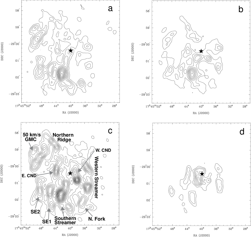
Figure 1: Velocity integrated maps of a) NH₃(1,1), b) NH₃(2,2), c) NH₃(3,3), and d) NH₃(6,6). Contours are in steps of 1.32 Jy beam^-1 km s^-1 in all four panels. The rms noise level, $\sigma_{JK}$, for each $(J,K)$ rotation inversion transition is $\sigma_{11}=0.28$ Jy beam^-1 km s^-1, $\sigma_{22}=0.30$ Jy beam^-1 km s^-1, $\sigma_{33}=0.33$ Jy beam^-1 km s^-1, and $\sigma_{66}=0.33$ Jy beam^-1 km s^-1 (McGary et al., 2001; Herrnstein & Ho, 2002). The position of Sgr A* is labeled by a star in each panel. The main molecular features in the central 10 pc are labeled in panel c.

Previous NH₃ observations detect a long filamentary “southern streamer” extending northwards from the “20 km s^-1” GMC (M–0.13–0.08; Güsten et al. (1981)) towards the the southeastern edge of the CND (Okumura et al., 1989; Ho et al., 1991; Coil & Ho, 1999, 2000). (See Figure 1c for positions of the main molecular features in the region.) Increased line widths and evidence of heating as the southern streamer approaches the Galactic center indicate that gas may be flowing from the 20 km s^-1 GMC towards the circumnuclear region. Supporting morphological evidence for this connection has come from observations of HCN(3–2) (Marshall et al., 1995), ¹³CO(2–1) (Zylka et al., 1990), and 1 mm continuum emission (Dent et al., 1993; Zylka et al., 1998). However, the southern streamer shows neither the velocity gradient nor curved morphology that would be expected for a cloud infalling towards the nucleus (Coil & Ho, 1999). NH₃ emission also becomes very faint near the CND making it difficult to study the gas in this region (McGary et al., 2001). Two additional connections originating in the northern fork of the 20 km s^-1 GMC (Coil & Ho, 1999, 2000) and the northern ridge (McGary et al., 2001) have also been suggested based on NH₃ observations. A fourth possible connection originating in the “50 km s^-1” GMC (M–0.03–0.07) was detected in HCN(1–0), but it has not been observed in NH₃ (Ho, 1995).

In this paper, we combine data from previous interferometric observations of four rotation inversion transitions of NH₃ to study the molecular environment in this region in detail. The observations and velocity integrated maps, which were previously published in McGary et al. (2001) and Herrnstein & Ho (2002), are briefly reviewed in §2. We then derive physical parameters for the molecular clouds in §3, and use these results to investigate the impact of Sgr A East on molecular gas in the central 10 pc in §4. Based on the interaction of Sgr A East with the western streamer, we place limits on the energy of the progenitor explosion. In §5, we discuss the detailed temperature structure of molecular clouds at the Galactic center. Measured temperatures for clouds more than 2 pc from Sgr A* are consistent with a two-temperature structure in which roughly one quarter of the gas is contained in a hot ($\sim 200$ K) component. This structure is similar to the model used by Hüttemeister et al. (1993a) to characterize temperatures on larger scales. NH₃ (6,6)-to-(3,3) line ratios in the central 2 pc, however, exceed theoretical limits for gas in LTE (Herrnstein & Ho, 2002). In §5.2, we model these line ratios as resulting from absorption of NH₃(3,3) by cool material in a shielded layer of the cloud. In §6, we disentangle emission from three distinct molecular clouds within a projected distance of 2 pc from Sgr A* through a comparison of NH₃(3,3) and (6,6) emission. We conclude this paper with a model of the line-of-sight (LOS) distribution of the main features in the central 10 pc based on our molecular data and in the context of existing data at other wavelengths.

2 Observations and Velocity Integrated Maps

The large range of velocities observed at the Galactic center and the relatively narrow velocity coverage of current interferometers at centimeter wavelengths make spectral line observations of the region difficult. A velocity coverage of $\pm 110$ km s^-1 is necessary to detect all of the emission from the CND, but additional clouds with velocities as high as –185 km s^-1 have been detected near Sgr A* (Zhao et al., 1995). Using the Very Large Array (VLA), we observed the central 10 pc of the Galaxy in NH₃(1,1), (2,2), and (3,3) in 1999 March. The five pointing mosaic fully samples the central $5^{\prime}$ (10 pc) of the Galaxy with a velocity coverage of of –140 to +130 km s^-1. The resulting data are more complete in both velocity coverage and spatial sampling than previous interferometric observations of NH₃ emission in this region, which tended to concentrate on velocities associated with the GMCs (Coil & Ho, 1999). However, the wide velocity coverage of our data is gained at the expense of channel width, which is only 9.8 km s^-1.

Figure 1a-c shows velocity integrated maps of NH₃(1,1), (2,2), and (3,3) emission from the central 10 pc (see McGary et al. (2001) for details on the observational setup and data reduction). The position of Sgr A* ($\alpha_{2000}=17^{h}45^{m}40^{s}.0,~{}\delta_{2000}=-29^{\circ}00^{\prime}26^{\prime\prime}.6$) is marked by a star in each panel. Major molecular features discussed in this paper are labeled in Figure 1c. After application of a Gaussian taper to de-emphasize long baselines, the synthesized beam in all three maps is roughly $16^{\prime\prime}\times 14^{\prime\prime}$ with a position angle of $\sim 0^{\circ}$. The rms noise level, $\sigma_{JK}$, for each $(J,K)$ rotation inversion transition is $\sigma_{11}=0.28$ Jy beam^-1 km s^-1, $\sigma_{22}=0.30$ Jy beam^-1 km s^-1, and $\sigma_{33}=0.33$ Jy beam^-1 km s^-1 (McGary et al., 2001). Contours in all four panels of Figure 1 are in steps of 1.32 Jy Beam^-1 km s^-1, thereby facilitating comparisons between different transitions. However, all emission exceeding $3\sigma_{JK}$ is considered significant (see McGary et al. (2001) for maps showing $3\sigma_{JK}$ contours). In order to have a constant noise level across the map, we have not corrected for primary beam attenuation at the edge of our mosaic, and the data are not sensitive to emission $\lower 2.15277pt\hbox{$\;\buildrel>\over{\sim}\;$}150^{\prime\prime}$ from Sgr A* (McGary et al., 2001). The 50 km s^-1 GMC, molecular ridge (composed of SE1 and SE2), and southern streamer all extend past the edge of the mosaic (see Armstrong & Barrett, 1985; Dent et al., 1993; Zylka et al., 1998, for large-scale maps showing the extent of these clouds). However, the outer edges of both the northern ridge and western streamer occur well within our mosaic and reflect intrinsic cloud edges (McGary et al., 2001).

As reported in McGary et al. (2001), we find dense molecular gas throughout much of the region. A notable exception is the far western and northwestern parts of the mosaic. These regions also lack emission from HCN(1–0) (Wright et al., 2001) and thermal dust (Dent et al., 1993; Zylka et al., 1998; Pierce-Price et al., 2000). Emission from NH₃ is predominately associated with the 20 and 50 km s^-1 GMCs. Both the southern streamer and northern fork (Coil & Ho, 1999) are extensions of the 20 km s^-1 GMC. The two southeastern clouds (SE1 and SE2) form part of the “molecular ridge” that connects this GMC to the 50 km s^-1 GMC in the northeast (Coil & Ho, 2000). Only the CND, northern ridge, and western streamer show velocities outside the $\sim 20-50$ km s^-1 range, and are not direct extensions of these GMCs. Overall, we find some evidence for kinematic connections between giant molecular clouds in the central 10 pc, but the expansion of the Sgr A East shell appears to be a dominating force in the region, possibly pushing much of the molecular gas away from the nucleus (McGary et al., 2001; Herrnstein & Ho, 2003).

In 2001, an upgrade of the 23 GHz system at the VLA enabled us to make the first interferometric map of the Galactic center in NH₃(6,6) ($\nu=25.056025$ GHz). With an energy above ground of 412 K, NH₃(6,6) traces significantly warmer gas than our earlier NH₃ data. An identical setup to our previous NH₃ observations was used. After application of a Gaussian taper to the $(u,v)$ data, the resulting synthesized beam is $16^{\prime\prime}\times 14^{\prime\prime}$ (Herrnstein & Ho, 2002). A velocity integrated map of NH₃(6,6) emission is shown in Figure 1d. Contour levels are the same as in panels a–c, and correspond to steps of $4\sigma_{66}$, where $\sigma_{66}=0.33$ Jy Beam^-1 km s^-1. While some features such as the western streamer are also observed in lower NH₃ rotation inversion transitions, the velocity integrated image is dominated by a cloud of hot molecular gas located less than 2 pc in projected distance from Sgr A*. This cloud is apparently located interior to the CND, and fills the molecular “hole” in the NH₃(3,3) map (Herrnstein & Ho, 2002).

3 Derived Parameters

3.1 Opacity and Intrinsic Line Width

Hyperfine splitting of the NH₃ rotation inversion transitions enables direct calculation of gas opacity (Ho & Townes, 1983). Each NH₃ rotation inversion transition is split into five hyperfine components by the interaction between the electric quadrupole moment of the nitrogen nucleus and the electric field of the electrons (see Townes & Schawlow (1975) and Ho & Townes (1983) for a detailed description of the NH₃ rotation inversion transitions). Although spin-spin interactions further split each of these components, the resulting lines are closely spaced in frequency and are only resolvable in cold, quiescent cores where line widths are less than 1–2 km s^-1. Therefore, the spectral profile for a typical molecular cloud with a line width of a few kilometers per second will consist of a main line and two symmetric pairs of satellite hyperfine lines, which are located 10–30 km s^-1 from the main line. At the Galactic center, however, molecular clouds have line widths in excess of 10 km s^-1, and even the five electric quadrupole components are blended. The blending of these components produces a correlation between measured line widths of the gas and calculated main line opacities (McGary & Ho, 2002).

In McGary & Ho (2002), we presented a method to disentangle the opacity and intrinsic line width by using the observed line widths ($\Delta\rm{v}_{obs}$) and main line flux densities of two rotation inversion transitions. In that paper, we used NH₃(1,1) and (3,3) because they had the highest signal-to-noise (S/N) (see Figure 1). However, as a result of their different excitation requirements, the NH₃(3,3) and (1,1) lines do not in fact trace the same volume of gas at the Galactic center (see §5.1). We have recalculated the NH₃(1,1) main line opacity ($\tau_{\rm{m}}(1,1)$) and $\Delta\rm{v}_{int}$ using the NH₃(1,1) and (2,2) data. With an energy difference of only 42 K, NH₃(1,1) and (2,2) are more likely to trace the same material. NH₃(2,2) is significantly fainter than NH₃(3,3), and the lower S/N limits somewhat the number of pixels to which our method can be applied.

In addition to changing the two rotation transitions considered in our method, we also use a Monte-Carlo simulation with 1000 trials to determine the significance of the derived parameter value at every pixel. Solutions are calculated following the algorithm of McGary & Ho (2002) for every pixel with a $>3\sigma$ detection of both the (1,1) and (2,2) lines and an uncertainty in the observed line width of $<20$ km s^-1. Uncertainties in the measured flux densities are equal to the rms noise in the map, and uncertainties in the observed line widths are estimated from the fit of a Gaussian profile to the spectrum. Pixels included in the final map must successfully converge in at least 50% of the trials. The exact value of this cutoff does not appear to be important, and all pixels with solutions $>50\%$ of the time show similar trends.

For each pixel, the final value for the parameter is taken to be the mean value from the Monte-Carlo simulations. The mean values of $\Delta\rm{v}_{obs}$ and $\tau_{\rm{m}}(1,1)$ at each pixel are plotted in Figure 2a and c. No smoothing has been applied to the data, and regions of low S/N have a “pixelated” appearance. Uncertainties in each parameter are calculated from the standard deviation of the distribution of solutions at each pixel. Figures 2b and d plot the S/N of $\Delta\rm{v}_{int}$ and $\tau_{\rm{m}}(1,1)$, respectively, at each pixel.

Table 1 lists the mean and standard deviation of derived parameters (including $\Delta\rm{v}_{int}$ and $\tau_{\rm{m}}(1,1)$) for the main molecular clouds in the central 10 pc. To avoid confusion with mean pixel values described above, we refer to the cloud-averaged value as the “characteristic value.” The characteristic parameter value is calculated as the average of the parameter at all pixels where a value was determined from the Monte-Carlo simulations with $>3\sigma$ significance. For the northern ridge and western streamer, some parameters had no determinations with $>3\sigma$ significance. In these cases, all pixels were used in the calculation of the characteristic value and standard deviation. Inclusion of all pixels will tend to lower the characteristic value because smaller values will have a lower significance for a given absolute uncertainty. The characteristic value quoted in Table 1 is intended to provide a general value that can be easily compared between different clouds. However, it is important to note that many parameters show significant variations, such as gradients and local maxima/minima, within a single cloud. The amount of significant variation of each parameter within a cloud is characterized by the standard deviation, which is also listed in Table 1.

Both the 50 km s^-1 GMC ($\Delta\alpha=120^{\prime\prime}$, $\Delta\delta=60^{\prime\prime}$) and the central region of the southern streamer ($30^{\prime\prime}$, $-90^{\prime\prime}$) have NH₃(1,1) main line opacities significantly greater than one (see Figure 2a). The characteristic opacity that we derive for the southern streamer is very similar to the values measured by Coil & Ho (1999). The western streamer and northern ridge have significantly lower opacities with typical values of $0.3-0.4$. Hatched regions in Figure 2b denote pixels for which only a lower limit for the opacity could be calculated. Although some of these values are the result of poor signal-to-noise, others may reflect real regions of high opacity. Many of these pixels have main line opacities near five, which corresponds to the maximum value of opacity considered in our solution method (McGary & Ho, 2002).

Intrinsic line widths in the central 10 pc tend to have values between 10 and 20 km s^-1 (see Figure 2c). Significant increases in intrinsic line widths are observable near many cloud edges. However, the apparent random distribution of these features throughout the central 10 pc makes it difficult to determine the exact way in which they formed. In general, these gradients may reflect dissipative effects at cloud edges possibly due to external pressures or tidal effects. For those pixels where only a lower limit on opacity can be calculated, the effect of blending on observed line width cannot be determined. The NH₃(2,2) observed line width is less affected by blending of the hyperfine lines than $\Delta\rm{v}_{obs}(1,1)$, and it is therefore used as the upper limit to the intrinsic line width for these pixels (Herrnstein, 2003).

Using the derived values of $\tau_{\rm{m}}(1,1)$ and $\Delta\rm{v}_{int}$ along with the measured main line fluxes, we can calculate the (2,2)-to-(1,1) rotational temperature, excitation temperature, and column density, and ultimately estimate cloud masses. In the derivation of each parameter, we perform a Monte-Carlo simulation to determine the mean value and associated uncertainties at each pixel. Pixels for which only a limiting value was calculated for $\tau_{\rm{m}}(1,1)$ and $\Delta\rm{v}_{int}$ are not included in the following calculations.

3.2 Rotational and Excitation Temperatures

The ratio of main line emission from two NH₃ rotation inversion transitions can be used to calculate the rotational temperature of molecular clouds at the Galactic center. From Ho & Townes (1983), the equation for rotational temperature calculated using NH₃(1,1) and (2,2) is

$$T_{R21}=\frac{-41.5~{}\rm{K}}{{\rm ln}\left(\frac{-0.282}{\tau_{m}(1,1)}{\rm ln}\left(1-\frac{\Delta T_{A_{m}}(2,2)}{\Delta T_{A_{m}}(1,1)}\left(1-e^{-\tau_{m}(1,1)}\right)\right)\right)}~{},$$ (1)

where $\frac{\Delta T_{A_{m}}(2,2)}{\Delta T_{A_{m}}(1,1)}$ is the ratio of emission from NH₃(2,2) and (1,1) main hyperfine lines. (Because of the similar frequencies of the NH₃ transitions, $\Delta T_{A}$ depends linearly on flux density, and the ratio of main line flux densities can be used in place of the ratio of antenna temperatures.) Using $\tau_{\rm{m}}(1,1)$ and the peak fluxes of the NH₃(1,1) and (2,2) emission, we calculate NH₃ (2,2)-to-(1,1) rotational temperatures. Mean values of $T_{R21}$ from the Monte-Carlo simulations and the associated S/N estimates are plotted in Figure 3a and b. In addition, Table 1 lists the characteristic (2,2)-to-(1,1) rotational temperature for each cloud.

(2,2)-to-(1,1) rotational temperatures in the central 10 pc are generally 25 K with uncertainties on the order of 10%. The relatively small uncertainties are the result of a weak dependence on $\tau_{\rm{m}}(1,1)$ for $0<\tau_{\rm{m}}(1,1)<1$ and (2,2)-to-(1,1) line ratios less than one (Ho & Townes, 1983). The derived rotational temperature depends primarily on the (2,2)-to-(1,1) line ratio, which is determined with a much higher S/N than $\tau_{\rm{m}}(1,1)$. The coldest gas is found in the 50 km s^-1 GMC ($120^{\prime\prime}$, $60^{\prime\prime}$), where the characteristic rotational temperature is $21$ K. The western streamer ($-80^{\prime\prime}$, $-40^{\prime\prime}$ and $-50^{\prime\prime}$, $40^{\prime\prime}$) has the warmest gas, with a characteristic (2,2)-to-(1,1) rotational temperature of $31$ K.

The measured rotational temperature is a lower limit on the true kinetic temperature of the gas (Martin et al., 1982). Table 1 lists the kinetic temperatures calculated from $\langle T_{R21}\rangle$ using the relations of Danby et al. (1988), which assume a H₂ density of $10^{5}$ cm^-3. (The degree to which $T_{R21}$ underestimates $T_{K}$ decreases as the H₂ density increases, until $T_{R21}\approx T_{K}$ for $n_{H_{2}}\lower 2.15277pt\hbox{$\;\buildrel>\over{\sim}\;$}10^{8}$ cm^-3 (Hüttemeister et al., 1993a).) The resulting range of kinetic temperatures for clouds in the central 10 pc is roughly 20–50 K. It is important to note that NH₃ (2,2)-to-(1,1) rotational temperatures are not sensitive to gas with kinetic temperatures much greater than 50 K (see Danby et al., 1988). Therefore, the true range of temperatures at the Galactic center is much larger than indicated by the (2,2)-to-(1,1) rotational temperatures in Figure 3a. This effect will be discussed in more detail in §5.1.

From standard radiative transfer, the excitation temperature is related to the measured antenna temperature of the line emission, $\Delta T_{A}$, by

$$\Delta T_{A}=\eta~{}\Phi~{}(T_{ex}-T_{bg})(1-e^{-\tau})$$ (2)

where $\eta$ is the telescope efficiency (0.4 for the VLA at 23 GHz), $\Phi$ is the filling factor, $T_{ex}$ is the excitation temperature of the gas, and $T_{bg}$ is the temperature of background radiation incident on the cloud (assumed to be the 2.7 K background of the Cosmic Microwave Background (CMB)). Solving for excitation temperature, we have

$$T_{ex}=2.7~{}{\rm K}+\frac{\Delta T_{A}}{\eta\Phi(1-e^{-\tau})}~{}.$$ (3)

Assuming the filling factor is equal to one (probably not a realistic assumption, see below), we have calculated the excitation temperature for gas in the central 10 pc. The resulting maps of mean excitation temperature and the S/N of these values determined from Monte-Carlo simulations are shown in Figure 3c and d. Overall, the excitation temperature has a smooth distribution (especially in regions with high S/N), with values ranging between 4 and 8 K. The characteristic excitation temperatures that we derive are consistent with the peak values reported by Coil & Ho (1999, 2000). Our results are also consistent with excitation temperatures of $\sim 5$ K derived from NH₃ observations within a few degrees of the Galactic center (Hüttemeister et al., 1993a).

Throughout the central 10 pc, calculated excitation temperatures are much lower than the corresponding (2,2)-to-(1,1) rotational temperatures. There are two possible explanations for this discrepancy. First, low densities could lead to sub-thermal excitation due to lack of collisions. From detailed balance of emission and absorption, the equation for $T_{ex}$ is

$$e^{-h\nu/k_{b}T_{ex}}=\frac{\frac{n(H_{2})}{n_{crit}}e^{-h\nu/k_{b}T_{K}}+u}{\frac{n(H_{2})}{n_{crit}}+u+1}~{},$$ (4)

where $k_{b}$ is the Boltzmann constant and $u=1/(e^{h\nu/k_{b}T_{rad}}-1)$ (see e.g. Stutzki & Winnewisser, 1985). The critical density is defined as the ratio of the Einstein coefficient for spontaneous emission to the collision coefficient. Using the values for $A_{10}$ from Ho & Townes (1983) and collision coefficients from Danby et al. (1988), we calculate a critical density of $2\times 10^{3}$ cm^-3 for every rotation inversion transition that we have observed. Figure 4 plots the excitation temperature as a function of H₂ volume density for selected kinetic temperatures. Despite the low critical density, excitation temperatures do not increase significantly until $n(H_{2})\approx 10^{5}$ cm^-3, and the gas is not thermalized ($T_{ex}\approx T_{K}$) until densities approach $10^{6}$ cm^-3. The large differences between our measured excitation and kinetic temperatures imply an H₂ density of $\lower 2.15277pt\hbox{$\;\buildrel<\over{\sim}\;$}10^{4}$ cm^-3, which is significantly lower than densities measured for the GMCs and CND. Sub-thermal excitation of this sort would imply even larger kinetic temperatures for molecular gas in the central 10 pc.

In §5.2, we will argue that at least the hottest gas components in the Galactic center must be nearly thermally excited with $n$(H₂)$\lower 2.15277pt\hbox{$\;\buildrel>\over{\sim}\;$}10^{5}$ cm^-3. A more likely cause of the low measured excitation temperatures is small filling factors. If the clouds fill only a small fraction of the beam, then the observed excitation temperature will be lowered by the ratio of the cloud area to the area of the beam. If the molecular gas in the central 10 pc is thermalized, then the measured difference between $T_{ex}$ and $T_{R21}$ implies typical filling factors of $\sim 0.2$.

3.3 Column Densities and Masses

The column density of a NH₃(J,K) rotation inversion transition is calculated as

$$N_{{\rm JK}}=4.1\times 10^{-20}~{}{\rm cm^{-2}}~{}\frac{\tau_{m}\nu^{2}T_{ex}\Delta{\rm v}}{A_{10}k_{{\rm JK}}}~{},$$ (5)

where $A_{10}$ is the Einstein coefficient for spontaneous emission and $k_{{\rm JK}}$ is the fraction of emission in the main hyperfine line (Ho et al., 1977; Herrnstein, 2003). For NH₃(1,1), $\nu=23.69$ GHz, $A_{10}=1.67\times 10^{-7}$ s^-1, and $k_{11}=0.50$. Thus Equation 5 becomes

$$N_{11}=2.8\times 10^{13}~{}{\rm cm^{-2}}~{}\tau_{m}(1,1)~{}T_{ex}~{}\left(\frac{\Delta{\rm v}}{1~{}{\rm km~{}s^{-1}}}\right)~{}.$$ (6)

The total NH₃ column density depends on $N_{11}$ and the fraction of molecules in the (1,1) state. The fraction of NH₃ molecules in the (J,K) state is

$$f_{{\rm JK}}=n_{\rm JK}/\sum\limits_{J=0}^{\infty}\sum\limits_{K=0}^{J}n_{{\rm JK}}~{},$$ (7)

where $n_{{\rm JK}}=g_{\rm JK}e^{-E_{{\rm JK}}/k_{b}T_{R}}$ is the number of molecules in the (J,K) state for a given rotational temperature (Townes & Schawlow, 1975). The energy above ground of a (J,K) rotation inversion transition is $E_{{\rm JK}}=h\left(BJ(J+1)+(C-B)K^{2}\right)$, where $B=h/8\pi^{2}I_{B}=2.98\times 10^{11}$ Hz and $C=h/8\pi^{2}I_{C}=1.89\times 10^{11}$ Hz. Given $f_{JK}$ and $N_{JK}$, the total NH₃ column density is then $N_{{\rm NH_{3}}}=N_{JK}/f_{JK}$. For NH₃(1,1), $E_{11}/k_{b}=23$ K. We have chosen to consider only the lowest 19 metastable states of NH₃ in calculating the fractional population of the NH₃(1,1) transition. The time scale for spontaneous emission for the non-metastable states is roughly one second, six orders of magnitude shorter than that for metastable states. However, emission from these states has been detected from the nearby Sgr B2 region . The omission of non-metastable states from our calculation will at most cause an overestimation of the fractional population of a factor of two (Herrnstein, 2003).

The NH₃(1,1) column density is related to $\tau_{\rm{m}}(1,1)$, $T_{ex}$, and $\Delta\rm{v}_{int}$ by (Ho et al., 1977)

$$N_{11}=2.8\times 10^{13}~{}{\rm cm^{-2}}~{}\tau_{m}(1,1)~{}T_{ex}~{}\left(\frac{\Delta{\rm v}}{1~{}{\rm km~{}s^{-1}}}\right)~{}.$$ (8)

By correcting for the fraction of molecules in the (1,1) state, which is characterized by the rotation temperature, $N_{11}$ can be converted to the total NH₃ column density, $N_{\rm{NH_{3}}}$ (Townes & Schawlow, 1975). Although emission from non-metastable states has been observed from the nearby Sgr B2 star-forming region (Hüttemeister et al., 1993b), we consider only the lowest 19 metastable states of NH₃ in our calculation of the fractional population of the NH₃(1,1) transition. The omission of non-metastable states from our calculation will at most cause an overestimation of the fractional population of a factor of two (Herrnstein, 2003).

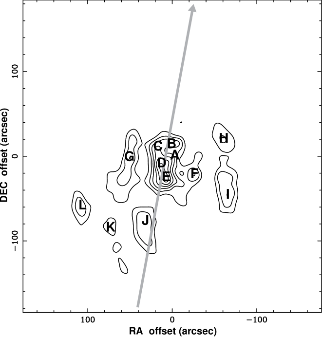
Figure 9: Position of twelve spectra and one position-velocity cut overlaid on a velocity integrated map of NH₃(6,6). Sgr A* is located at ($\Delta\alpha=0^{\prime\prime}$,$\Delta\delta=0^{\prime\prime}$) (spectrum A).

Total NH₃ column densities determined from our data are plotted in Figure 5 and characteristic values for specific clouds are listed in Table 1. Characteristic column densities for the main features range from $2-9\times 10^{15}$ cm². However, the largest column densities ($N_{{\rm NH_{3}}}>10^{16}$ cm²) are found primarily in the features associated with the GMCs. The central core of the southern streamer ($30^{\prime\prime}$, $-80^{\prime\prime}$) has a NH₃ column density of $1.4(\pm 0.3)\times 10^{16}$ cm^-2. The 50 km s^-1 GMC also has large NH₃ column densities, with highest values found at the northeastern edge of our mosaic. This GMC extends more than an arcminute past the northeastern edge of our map (see Figure 9 in McGary et al. (2001)), and emission at ($-130^{\prime\prime}$, $80^{\prime\prime}$) is associated with dense regions of the cloud where column densities should be highest.

At the Galactic center, the total mass of a cloud is given by

$$M=2.4~{}{\rm M_{\odot}}~{}\left(\frac{N_{{\rm NH_{3}}}}{10^{15}~{}{\rm cm}^{-2}}\right)\left(\frac{A}{1~{}\Box^{\prime\prime}}\right)\left(\frac{X{\rm(NH_{3})}}{10^{-7}}\right)^{-1}~{}.$$ (9)

where $A$ is the area of the cloud in arcsec² and $X$(NH₃) is the abundance of NH₃ relative to H₂. At present, $X$(NH₃) is not well-known for Galactic center molecular clouds. Abundances measured in the Perseus and –3 km s^-1 spiral arms and in dense, star-less cores suggest $X$(NH₃)$=10^{-9}-10^{-8}$ (Benson & Myers, 1983; Batrla et al., 1984; Serabyn & Guesten, 1986). However, there is much evidence that NH₃ abundances are enhanced in warm clouds, most likely as the result of evaporation of NH₃ molecules off of dust grains (Pauls et al., 1983; Walmsley et al., 1987). NH₃ abundances range from $10^{-7}$ to $10^{-4}$ in warm molecular clouds, with the highest measured abundances coming from the Sgr B2 complex, one of the largest star formation regions in the Galaxy (Hüttemeister et al., 1993b, and references therein). The precise relationship between $X$(NH₃) and $T_{K}$ is not straightforward. Assuming that high temperatures at the Galactic center will produce enhanced abundances of NH₃, we adopt $X$(NH₃)=$10^{-7}$ in our calculations. Resulting estimates of masses are presented in Table 1. The assumption of an enhanced NH₃ abundance should produce smaller cloud masses than those calculated by Coil & Ho (1999, 2000), who use $X$(NH₃)$=10^{-8}$.

A comparison of our derived mass for the edge of the 50 km s^-1 GMC to published values in the literature can be used as a consistency check for our choice of $X$(NH₃). Total mass estimates for the 50 km s^-1 GMC range between $6\times 10^{4}$ and $4\times 10^{5}$ $M_{\odot}$ (Güsten et al., 1981; Armstrong & Barrett, 1985; Zylka et al., 1990). The virial relation between the mass of a cloud and its size and line width ($M_{V}\approx 2\times 10^{2}~{}{\rm M_{\odot}}~{}\left(\frac{R}{1~{}{\rm pc}}\right)\left(\frac{\Delta{\rm v}}{1~{}{\rm km~{}s}^{-1}}\right)^{2}$ for a density profile of $1/r$, MacLaren et al. (1988)) can also be used to calculate the minimum mass of a gravitationally bound cloud. Assuming a size of 5 pc and a line width of 17 km s^-1 (see Table 1), the virial mass of the 50 km s^-1 GMC is $\sim 3\times 10^{5}$ $M_{\odot}$. As previously mentioned, roughly 3/4 of the 50 km s^-1 GMC, including the densest condensations, lies outside our VLA mosaic. Our derived mass of $5\times 10^{4}$ $M_{\odot}$ for the fraction of this cloud within our mosaic is therefore consistent with what we expect, and we conclude that $X$(NH₃)$=10^{-7}$ is a reasonable assumption for molecular clouds near Sgr A*.

The southern streamer is the second-most massive feature in the central 10 pc. We estimate a total mass of $8\times 10^{4}$ $M_{\odot}$ for the southern streamer. Using $X$(NH₃)$=10^{-8}$, Coil & Ho (1999) calculate a mass of $6\times 10^{4}$ $M_{\odot}$ for gas from the “central cloud” of the southern streamer, which is roughly coincident with the core of bright NH₃ emission centered at ($+30^{\prime\prime}$, $-80^{\prime\prime}$) in our maps. If the Coil & Ho (1999) result is re-calculated using our assumed value of X(NH₃) then the associated mass would be $6\times 10^{3}$ $M_{\odot}$, more than an order of magnitude smaller than our value. The large difference between these results reflects different definitions for the size and extent of the southern streamer. First, Coil & Ho (1999) assume a size of only 300 arcsec² for the central cloud, while it appears to be closer to 2000 arcsec² in our velocity integrated maps. In addition, the emission associated with the southern streamer at ($0^{\prime\prime}$, $-125^{\prime\prime}$) is associated with the northern tip of the “southern cloud” in Coil & Ho (1999) and not included in the above mass estimate. It should also be noted, that the measured NH₃ column for the central cloud is consistent between the two papers (for the same assumption of X(NH₃)). Considering the different assumptions outlined above, the reported masses for the southern streamer are consistent. However, we believe that our result is a more complete measure of the mass of the southern streamer from $50^{\prime\prime}$ to $150^{\prime\prime}$ south of Sgr A*.

— to be cut

and $2.3\times 10^{5}$ $M_{\odot}$ for gas from the extended “southern cloud”, centered roughly 150^′′ south of Sgr A*. The majority of the “southern cloud” is outside of our VLA mosaic. Due to the assumption of a lower NH₃ abundance, these masses should be expected to be roughly an order of magnitude smaller than our derived mass.

However, we can calculate a mass associated with the “central cloud” alone. Using the characteristic value of $N_{NH_{3}}$ from Table 1, and assuming a size of only 1600 arcsec², we calculate a mass of $3.3\times 10^{4}$ M_⊙.

located roughly at ($+30^{\prime\prime}$, $-80^{\prime\prime}$). This position corresponds to the core of bright emission that we detect from the southern streamer. the southern streamer associated Because (Coil & Ho, 1999) do not convert $\tau_{\rm{m}}(1,1)$ to the total opacity across all hyperfine lines ($\tau$(1,1)), the correct mass estimate for their data should be $1.2\times 10^{5}$ $M_{\odot}$. Considering the different assumptions for $X$(NH₃), our derived mass for the southern streamer is significantly larger than that derived by (Coil & Ho, 1999). The larger mass estimate from our data may imply that we recovered more flux in our de-convolution algorithm, which used maximum entropy rather than CLEAN (McGary et al., 2001).

—-

We estimate masses of $1\times 10^{4}$ $M_{\odot}$ and $2\times 10^{4}$ $M_{\odot}$ for SE1 and SE2, respectively. Together, these clouds have a mass of a few$\times 10^{4}$ $M_{\odot}$, and constitute the majority of the dense “molecular ridge” that connects the 20 km s^-1 GMC in the south to the 50 km s^-1 GMC in the northeast (Coil & Ho, 2000). Both the western streamer and northern ridge have masses roughly an order of magnitude smaller than the southern streamer and two orders of magnitude smaller than estimated total masses of the 20 and 50 km s^-1 GMCs (Zylka et al., 1990). As we argue in the following section, we believe these smaller clouds have been swept up by the expansion of Sgr A East.

4 The Impact of Sgr A East on Nearby Molecular Clouds

Maps of radio continuum emission from the Galactic center show a large shell of synchrotron emission with a radius of $\sim 1.6^{\prime}$ (4 pc) centered roughly $1^{\prime}$ to the east of Sgr A* (Pedlar et al., 1989). This shell is called Sgr A East and is thought to lie within a few parsecs of the Galactic center (see §7). To the northeast, the edge of Sgr A East lies precisely along the western edge of the 50 km s^-1 GMC, and it is generally agreed that Sgr A East is interacting with the GMC to some extent. Previous work by Mezger et al. (1989) interpreted this interaction as indicating that much of the material in the 50 km s^-1 GMC was cleared out of the central parsecs by the expansion of Sgr A East. The resulting estimate of the energy of Sgr A East is $\lower 2.15277pt\hbox{$\;\buildrel>\over{\sim}\;$}4\times 10^{52}$ ergs, more than an order of magnitude larger than typical supernova remnants (Mezger et al., 1989). This result has sparked many discussions on the possible origin of Sgr A East, including multiple correlated supernovae, expansion within a bubble (Mezger et al., 1989), or tidal disruption of a star by the supermassive black hole (Khokhlov & Melia, 1996).

The assumption that a significant amount of material in the 50 km s^-1 GMC was swept up by the expansion of Sgr A East was based primarily on the apparent concave morphology of the GMC, with the northern part of the cloud wrapping around the top of the Sgr A East shell (Mezger et al., 1989). However, in McGary et al. (2001), we showed that this “northern ridge” is kinematically distinct from the 50 km s^-1 GMC, with a characteristic velocity of –10 km s^-1. Using the derived cloud parameters presented in the previous sections, we no longer need to rely on morphology as the primary indication of an interaction. In the following paragraphs, we revisit the question of the impact of Sgr A East on molecular gas near Sgr A*, and we calculate a new estimate for the energy associated with the progenitor explosion.

The 50 km s^-1 GMC, northern ridge, and western streamer lie along the edge of Sgr A East (McGary et al., 2001). However, the physical conditions differ significantly between these clouds. The molecular gas in the 50 km s^-1 GMC does not appear to be strongly affected by the impact of Sgr A East. The characteristic (2,2)-to-(1,1) rotational temperature of the 50 km s^-1 GMC ($\langle T_{R21}\rangle=21$ K) is the lowest value of any feature in the central 10 pc. If the 50 km s^-1 GMC is moving outwards with the expansion of Sgr A East, then we should expect to see a velocity gradient along the cloud. However, no velocity gradient is observed in this cloud (McGary et al., 2001).

The northern ridge and western streamer are more than a magnitude less massive than the 50 km s^-1 GMC, and thus might be expected to be more affected by the impact of Sgr A East. The northern ridge is a linear feature, roughly $90^{\prime\prime}$ in length, that lies along the northern edge of Sgr A East. Compared to the 50 km s^-1 GMC, the northern ridge has a similar characteristic intrinsic line width ($\langle\Delta\rm{v}_{int}\rangle=17$ km s^-1) and higher characteristic (2,2)-to-(1,1) rotational temperature ($\langle T_{R21}\rangle=28$ K). There is no velocity gradient larger than the size of the spectral resolution in our data ($\sim 9.8$ km s^-1), but this result is not surprising because the cloud velocity of –10 km s^-1 is consistent with the bulk of any expansion occurring perpendicular to the LOS.

The strongest evidence for an interaction between Sgr A East and molecular gas comes from the western streamer. The western streamer also has a long, filamentary structure, and its curvature matches closely the western edge of Sgr A East. In McGary et al. (2001) we reported a velocity gradient of 1 km s^-1 arcsec^-1 (25 km s^-1 pc^-1) covering 150^′′ (6 pc) along the western streamer. At ($60^{\prime\prime}$, $-80^{\prime\prime}$) emission is at $-70$ km s^-1, but the velocity smoothly shifts towards the red until it reaches $\sim 90$ km s^-1 at ($-70^{\prime\prime}$, $70^{\prime\prime}$) (McGary et al., 2001). A velocity gradient of this type is consistent with a ridge of gas highly inclined to the line-of-sight that is being pushed outwards by expansion of Sgr A East. In this model, the southern part of the streamer would be located on the front side of the shell, thereby producing the observed blue-shifted velocities. Molecular gas in the western streamer has the largest characteristic intrinsic line width ($20$ km s^-1) and highest temperatures in the central 10 pc. The characteristic (2,2)-to-(1,1) rotational temperature of $31$ K corresponds to a kinetic temperature near 46 K. The western streamer is also the only one of these three clouds with strong NH₃(6,6) emission, and it is likely that some fraction of the gas has kinetic temperatures $\lower 2.15277pt\hbox{$\;\buildrel>\over{\sim}\;$}100$ K.

Based on the above comparison, it seems unlikely that a significant amount of the 50 km s^-1 GMC has been moved by Sgr A East. However, there is convincing evidence that the expansion of Sgr A East swept up the material in the western streamer. Assuming that only the western streamer was cleared out of the central parsecs by Sgr A East, we calculate a new estimate of the age and energy of the progenitor explosion in the following paragraphs.

A supernova remnant (SNR) is reckoned to have entered the isothermal or “snow-plow” phase when the time scale for radiative cooling becomes less than the dynamical time of the SNR. At this point, the shell expands with constant radial momentum, and a thin, dense layer of gas is formed that moves outwards with the shock front. For a SNR in the snow-plow phase, the energy of the progenitor supernova, $E_{SN}$, is related to the current energy associated with the shell, $E_{sh}$, by (Shull, 1980)

$$\left(\frac{E_{SN}}{E_{sh}}\right)=\left(\frac{R_{sh}}{R_{sg}}\right)^{2}~{},$$ (10)

where $R_{sh}$ is the radius of the shell and $R_{sg}$ is the radius at the time of shell generation, $t_{sg}$. The shell radius at time, $t$, is given by (Shull, 1980)

$$R_{sh}=3.29~{}{\rm pc}~{}\left(\frac{E_{SN}}{10^{51}~{}{\rm ergs}}\right)^{\frac{1}{4}}\left(\frac{n_{o}}{100~{}{\rm cm}^{-3}}\right)^{-\frac{1}{2}}\left(\frac{t}{t_{sg}}\right)^{\frac{2}{7}}~{},$$ (11)

where $n_{o}$ is the mean initial H density in cm^-3. At $t=t_{sg}$, Equation 11 defines the shell generation radius, $R_{sg}$. Substituting the equation for $R_{sg}$ into Equation 10, and solving for $E_{SN}$ we find

$$E_{SN}=2.0\times 10^{50}~{}{\rm ergs}~{}\left(\frac{E_{sh}}{10^{51}~{}{\rm ergs}}\right)^{\frac{2}{3}}\left(\frac{R_{sh}}{1~{}{\rm pc}}\right)^{\frac{4}{3}}\left(\frac{n_{o}}{100~{}{\rm cm}^{-3}}\right)^{\frac{2}{3}}~{}.$$ (12)

If the $4\times 10^{3}$ $M_{\odot}$ of material in the western streamer was swept out of a region with a radius of 4 pc, then the implied mean initial density is $n_{o}\approx 600$ cm^-3, which is typical of molecular clouds. The kinetic energy associated with the western streamer (assuming a velocity of 100 km s^-1 (McGary et al., 2001)) is $E_{ws}=4\times 10^{50}$ ergs. Taking $E_{ws}$ as the shell energy, the derived energy for the progenitor supernova explosion is $E_{SN}=2\times 10^{51}$ ergs. This estimate of $E_{SN}$ is a lower limit on the energy of the progenitor explosion because the western streamer covers only a fraction of the total shell. The shell energy (and therefore $E_{SN}$) will scale as $4\pi/\Omega_{ws}$, where $\Omega_{ws}$ corresponds to the solid angle initially covered by the material in the western streamer. This solid angle likely differs significantly from the solid angle that it currently covers. For example, as the shock front expanded, it may have wrapped around the densest regions compressing them into narrow filaments and thereby decreasing the solid angle of the material in the western streamer. Based on observations of ionized material surrounding Sgr A East, the total kinetic energy of the shell has been estimated to be $\sim 2\times 10^{51}$ ergs (Mezger et al., 1989; Genzel et al., 1990). This kinetic energy would imply that $\Omega_{ws}/4\pi\approx 0.15$. The mean initial density calculated from the western streamer is also a lower limit. However, the observed distribution of dense molecular gas in the region indicates that Sgr A East probably expanded into a clumpy and highly non-homogeneous environment. The filaments of dense gas detected in NH₃ emission therefore likely account for the majority of the gas mass surrounding the remnant, and the estimate of $n_{o}$ from the western streamer is probably accurate to within a factor of a few. Taking $E_{sh}=2\times 10^{51}$ ergs and assuming $n_{o}=1000$ cm^-3, we calculate an upper limit on the energy of the progenitor supernova of $E_{SN}=9\times 10^{51}$ ergs.

Based on the range of energies for the progenitor explosion calculated from our molecular data, we conclude that Sgr A East is most likely the result of a single supernova that occurred near the Galactic center. The expansion of Sgr A East into molecular gas produced the western streamer and possibly the northern ridge, but it has had little effect on the majority of the material in the 50 km s^-1 GMC. In fact, this GMC is likely significantly slowing the expansion of the supernova remnant to the northeast of Sgr A*.

The case for a single supernova explosion as the progenitor of Sgr A East has been gaining momentum in the past few years. In particular, the small gas mass and thermal energy of $10^{49}$ ergs inferred from Chandra observations of hot gas associated with Sgr A East is consistent with the ejecta of a single supernova (Maeda et al., 2002). Based on the centrally concentrated X-ray emission, Maeda et al. (2002) classify Sgr A East as a “mixed morphology” (MM) SNR produced by a Type II supernova. This classification is supported by the detection of multiple 1720 MHz OH masers, which are often found in MM SNRs, along the edge of the shell (Yusef-Zadeh et al., 1999; Green et al., 1997).

Using the estimated energy of the progenitor supernova, we can calculate the age of Sgr A East. From Shull (1980), the time of shell generation is given by

$$t_{sg}=3600~{}{\rm yr}~{}\left(\frac{E}{10^{51}~{}{\rm ergs}}\right)^{\frac{1}{8}}\left(\frac{n_{o}}{100~{}{\rm cm}^{-3}}\right)^{-\frac{3}{4}}~{}.$$ (13)

Substituting the equation for $t_{sg}$ into Equation 11, we determine an age of $(1-2)\times 10^{4}$ yr for Sgr A East. This age is similar to the age of $7500$ yr derived by Mezger et al. (1989) for a model in which the supernova occurred within a low-density bubble inside the dense 50 km s^-1 GMC. However, the lack of evidence for a strong impact on the 50 km s^-1 GMC leads us to favor a scenario in which the supernova occurred outside the GMC. Our derived age of $\sim 10^{4}$ yr agrees well with other independent measurements of the age of Sgr A East. Based on the expected differential shearing of a shell near the Galactic center, Uchida et al. (1998) independently derive an age of a few $10^{4}$ year for Sgr A East. An age of $10^{4}$ yr is also consistent with the X-ray properties of the shell (Maeda et al., 2002).

As noted elsewhere (see e.g. Serabyn et al., 1992; Morris & Serabyn, 1996; Maeda et al., 2002) the inferred age of the supernova is 1–2 orders of magnitude smaller than the age of the Hii regions that lie along the western edge of the 50 km s^-1 GMC. Therefore, these Hii regions could not have been triggered by the impact of the Sgr A East shock front on the molecular cloud. However, the alignment of these star formation regions along the edge of the 50 km s^-1 GMC is noteworthy, and may be the result of previous interactions between this cloud and expanding shock fronts that originated near the nucleus.

5 The Temperature Structure of the Central 10 pc

5.1 A Two-Temperature Gas

In general, a rotational temperature can be calculated from any two rotation inversion transitions of NH₃ using the equation

$$T_{Rul}=\frac{-\Delta E_{ul}}{{\rm ln}\left[\frac{-C_{ul}}{\tau_{m,l}}{\rm ln}\left[1-\frac{\Delta T_{A_{m}}(u,u)}{\Delta T_{A_{m}}(l,l)}\left(1-e^{-\tau_{m,l}}\right)\right]\right]}~{},$$ (14)

where $\Delta E_{ul}$ is the energy difference between the upper ($J,K=u$) and lower ($J,K=l$) rotation inversion states and $C_{ul}=\frac{g_{l}|\mu_{10}|_{l}^{2}k_{l}}{g_{u}|\mu_{10}|_{u}^{2}k_{u}}$ relates the statistical weights ($g_{i}$), magnetic dipole moment ($|\mu_{10}|_{i}^{2}$), and fraction of emission in the main line ($k_{i}$) of the two transitions. This equation assumes equal excitation temperatures, filling factors, and telescope efficiencies for the two transitions. Due to slow mixing rates ($\sim 10^{-6}$ yr^-1) between the “ortho” ($K=3n$) and “para” ($K\neq 3n$) spin states of NH₃, rotational temperatures are generally calculated using two transitions from the same spin state (Ho & Townes, 1983). Therefore, if the gas is in LTE, then we can calculate a (6,6)-to-(3,3) rotational temperature from our VLA data.

NH₃ (6,6)-to-(3,3) line ratios in the central 10 pc are higher than would be expected based on NH₃ (2,2)-to-(1,1) rotational temperatures (Herrnstein & Ho, 2002). Within 2 pc of Sgr A*, the (6,6)-to-(3,3) line ratios exceed theoretical limits, preventing calculation of $T_{R63}$ (Herrnstein & Ho, 2002; Herrnstein, 2003). These “un-physical” line ratios will be explained in §5.2. Elsewhere in the map, faint NH₃(6,6) emission makes calculation of $T_{R63}$ difficult (see Figure 1). In addition, the NH₃(3,3) main line opacity cannot be reliably calculated from $\tau_{\rm{m}}(1,1)$ because these two transitions likely trace gas at different temperatures (see below). Although $\tau_{\rm{m}}(3,3)$ is directly related to the ratio of the main and outer-most satellite hyperfine lines, the relative population of the satellite lines compared to the main line is only 0.008 (compared to 0.22 for NH₃(1,1)), (Townes & Schawlow, 1975)), and emission from the satellite hyperfine lines is generally below the rms noise level of our map.

Due to the above limitations, $T_{R63}$ can only be directly calculated for the core of the southern streamer and SE1. At ($33^{\prime\prime}$, $-75^{\prime\prime}$), the southern streamer has a measured NH₃ (6,6)-to-(3,3) line ratio of $0.16\pm 0.02$ and a NH₃(3,3) main line opacity of $\tau_{\rm{m}}(3,3)=2.5^{+0.4}_{-0.3}$. The inferred(6,6)-to-(3,3) rotational temperature of $T_{R63}=80\pm 5$ K corresponds to a kinetic temperature of $100^{+10}_{-~{}9}$ K for gas with a H₂ density of $10^{5}$ cm^-3 (Danby et al., 1988). In SE1 ($73^{\prime\prime}$, $-87^{\prime\prime}$), the NH₃(3,3) main line opacity is $3.6^{+1.7}_{-1.5}$. The (6,6)-to-(3,3) main line ratio of $0.27^{+0.6}_{-0.5}$ corresponds to $T_{R63}=88^{+22}_{-14}$ K and a kinetic temperature of $110^{+45}_{-20}$ K.

Lower limits on the kinetic temperature can be calculated in SE2 and the 50 km s^-1 GMC. In SE2 ($108^{\prime\prime}$,$-60^{\prime\prime}$), the NH₃(6,6)-to-(3,3) line ratio is $0.39^{+0.05}_{-0.04}$, and an upper limit of 1.5 is calculated for $\tau_{\rm{m}}(3,3)$. These values result in lower limits for the rotational and kinetic temperatures of $T_{R63}\lower 2.15277pt\hbox{$\;\buildrel>\over{\sim}\;$}120$ K and $T_{K}\lower 2.15277pt\hbox{$\;\buildrel>\over{\sim}\;$}190$ K. For the 50 km s^-1 GMC, NH₃(6,6) is only detected near ($112^{\prime\prime}$, $48^{\prime\prime}$). (Although significant, the velocity integrated NH₃(6,6) emission at this position does not exceed 1.32 Jy beam^-1 km s^-1 ($\approx 4\sigma_{66}$) and thus is not seen in Figure 1d.) At this position, the (6,6)-to-(3,3) line ratio is $0.16\pm 0.05$ and $\tau_{\rm{m}}(3,3)\lower 2.15277pt\hbox{$\;\buildrel<\over{\sim}\;$}2$. The inferred lower limits on the derived temperatures are $T_{R63}\lower 2.15277pt\hbox{$\;\buildrel>\over{\sim}\;$}75$ K and $T_{K}\lower 2.15277pt\hbox{$\;\buildrel>\over{\sim}\;$}90$ K. Due to low S/N and large line widths, the main line opacity cannot be estimated for the western streamer. The typical line ratio of 0.7 in this cloud implies an upper limit of $T_{R63}\lower 2.15277pt\hbox{$\;\buildrel<\over{\sim}\;$}230$ K (Herrnstein & Ho, 2002). This upper limit on the (6,6)-to-(3,3) rotational temperature provides little constraint on the kinetic temperature of the gas (Danby et al., 1988).

The kinetic temperatures derived above are significantly higher than those derived from NH₃ (2,2)-to-(1,1) line ratios. This discrepancy is indicative of a gas composed of a mixture of separate cool and hot components. If multiple temperature components are contained within the telescope beam, then emission from different rotation inversion transitions will not trace the same material, and the resultant measurement of kinetic temperature will depend strongly on the choice of rotation inversion transitions used in the calculation. Because the fractional population of the (J,K) state is a function of kinetic temperature, each NH₃(J,K) transition is most sensitive to gas at a particular temperature corresponding to the peak fractional population of that transition. The peak fractional population of NH₃(1,1) and (2,2) occurs around 20–30 K (see Herrnstein, 2003), making these transitions excellent tracers of cool molecular material. At kinetic temperatures greater than 50 K, however, $T_{R21}$ becomes insensitive to changes in $T_{K}$. All kinetic temperatures $\lower 2.15277pt\hbox{$\;\buildrel>\over{\sim}\;$}80$ K have (2,2)-to-(1,1) rotational temperatures between 40 and 60 K (Walmsley & Ungerechts, 1983; Ho & Townes, 1983; Danby et al., 1988). Higher transitions such as NH₃(3,3) and (6,6) have a small fractional population in cool clouds. (For example, only $\sim 1$ % of the NH₃ molecules are in the NH₃(6,6) state for gas at 50 K.) The fractional population rapidly increases towards higher temperatures, making it easier to detect the emission. In addition, $T_{R63}$ is much more sensitive to variations in kinetic temperatures between 50 and a few hundred Kelvin. While an increase in kinetic temperature from 100 to 200 K changes $T_{R21}$ by only a few degrees, $T_{R63}$ increases from 80 to 125 K.

Extensive single-dish observations of NH₃ rotation inversion transitions by Hüttemeister et al. (1993a) show that molecular clouds in the central $4^{\circ}\times 1^{\circ}$ of the Galaxy are best characterized by a two-temperature gas distribution on the scale of 3 pc (corresponding to the size of the NRAO 40-m primary beam). In general, 75% of the total column of NH₃ comes from a cool gas at 25 K, while the remaining 25% of the material is contained in a hot component with a temperature of roughly 200 K (Hüttemeister et al., 1993a). The uncertainty in these temperatures is roughly 30%, but the cold temperature matches well the observed dust temperature in the region.

Based on the temperatures calculated in this paper, it appears that a similar cloud structure is valid in the central 10 pc on a spatial scales of $\sim 0.5$ pc. In Figure 6a, we plot the inferred kinetic temperature as a function of rotational temperature for different combinations of hot and cold gas. The hot gas is assumed to be at 200 K based on the results of Hüttemeister et al. (1993a). The cold component is set at 15 K in order to be consistent with the kinetic temperatures inferred from our $T_{R21}$ measurements. Models for the derived rotational temperatures are plotted for cases in which the hot component comprises 0, 25, 50, 75, and 100% of the gas.

Mean kinetic temperatures derived from our data are overlaid in Figure 6a. The mean kinetic temperature derived from $T_{R21}$ is $26\pm 2$ K. The cold component therefore must have a kinetic temperature lower than $\sim 25$ K. The two measurements of $T_{R63}$ from our data have a weighted average of $101\pm 9$ K. Although the low measurements from $T_{R21}$ imply a lower temperature for the cold component than derived by Hüttemeister et al. (1993a), the data are consistent with their conclusions that roughly 25% of the gas is contained in a hot component.

In order to study the temperature structure in the central parsecs in more detail, we have compiled published NH₃ rotational temperatures from a $7.5^{\prime}\times 11^{\prime}$ ($17.5\times 25.5$ pc) region surrounding Sgr A* that includes both the 20 and 50 km s^-1 GMC. A summary of the references for the measurements, including the telescope and corresponding beam size, is given in Table 2, and the specific values for the rotational temperatures are listed in Table 3. Only one pointing from the large-scale survey by Hüttemeister et al. (1993a) is contained within this region.

Figure 7, overlays the position of each observation on a 1.2 mm continuum image showing bright dust emission from the GMCs and free-free emission from ionized arcs of Sgr A West (Zylka et al., 1998). For single-dish measurements (Figure 7a), the size of the circle corresponds to the FWHM telescope beam. Single-dish observations have focused primarily on the large GMCs, and pointings tend to be arranged parallel to the Galactic plane. The FWHM of the primary beam is plotted for each interferometric observation in Figure 7b. Both Coil & Ho (1999, 2000) and the data presented in this paper include a pointing centered on Sgr A*. For the interferometric data, independent temperature measurements may be made once per synthesized beam. However, Okumura et al. (1989) and Coil & Ho (1999, 2000) present calculated temperatures at selected positions only. We plot the synthesized beam for the NMA at the positions of rotational temperature measurements in Okumura et al. (1989). In Coil & Ho (1999, 2000), characteristic rotational temperatures are given for the main condensations and we report their estimated positions in Table 3.

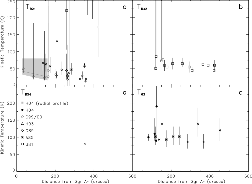
Figure 8: Measured kinetic temperature versus distance from Sgr A* calculated from the rotational temperatures listed in Table 3 using Danby et al. (1988). The four panels show kinetic temperatures derived from a) $T_{R21}$, b) $T_{R42}$, c) $T_{R54}$, and d) $T_{R63}$. Uncertainties in the radial distance from Sgr A*, which are equal to the FWHM of the beam, have been omitted for clarity. The dark grey line in panel $a$ shows the best fit radial profile for kinetic temperatures derived from our data. The surrounding light grey box shows the approximate range of kinetic temperatures from pixels with a significance of $\geq 3\sigma$.

Using the relation of Danby et al. (1988), kinetic temperatures have been calculated for all measurements of $T_{R21}$, $T_{R42}$, $T_{R54}$, and $T_{R63}$. ($T_{R41}$ is not included in Danby et al. (1988), and it is therefore not converted to a kinetic temperature.) In Figure 8, we plot kinetic temperatures as a function of distance from Sgr A*. The uncertainty in position due to the size of the beam (see Table 2) is not plotted. We also calculate a radial profile for the kinetic temperatures derived from our $T_{R21}$ measurements. The best fit radial profile $[T_{K}=31(\pm 2)-0.06(\pm 0.02)r]$ is overlaid as the grey line in Figure 8a. The surrounding light grey box shows the approximate range of derived kinetic temperatures from pixels with a $\geq 3\sigma$ determination of $T_{R21}$.

In general, kinetic temperatures in Figures 8a, b, and d are consistent with a relatively constant kinetic temperature within $500^{\prime\prime}$ of Sgr A*. Kinetic temperatures derived from our $T_{R21}$ measurements show a slight increase as gas nears Sgr A*. Unfortunately, there are no measurements of $T_{R63}$, which would be more sensitive to large increases in the kinetic temperature, within $100^{\prime\prime}$ of the nucleus. Kinetic temperatures derived from $T_{R63}$ for distances between $100^{\prime\prime}$ and $150^{\prime\prime}$ are consistent with measured kinetic temperatures at larger radii. Any significant heating of the molecular gas is therefore confined to a region less than $\sim 4$ pc from Sgr A*.

In Figure 6b, the average kinetic temperatures calculated from $T_{R21}$, $T_{R42}$, and $T_{R63}$ measurements in the central 20 pc are plotted as filled circles overlaid on the same models for a two-temperature gas as Figure 6a. These temperatures are calculated as the average of the measurements in Figure 8 weighted by the associated uncertainties (see Table 3), and are equal to $26\pm 6$ K, $55\pm 5$ K, and $100\pm 8$ K, for kinetic temperatures derived from $T_{R21}$, $T_{R42}$, and $T_{R63}$, respectively. (Values of $T_{R21}$ reported by Güsten et al. (1981) differ significantly from other published rotational temperatures (see Table 3) and imply extraordinarily high kinetic temperatures. Omission of these data from our analysis results in $\langle T_{R21}\rangle=24\pm 2$ K and does not affect the conclusions below.) The mean kinetic temperatures are consistent with the kinetic temperatures measured from our VLA data alone. Based on the consistency between our VLA measurements and these previously published results, we conclude that molecular clouds within 10–20 pc of Sgr A* have a two-temperature structure on size scales of $\lower 2.15277pt\hbox{$\;\buildrel<\over{\sim}\;$}0.5$ pc in which roughly one quarter of the gas is contained in a hot component.

Only one measurement of $T_{R54}$ has been made near the 20 or 50 km s^-1 GMC (Hüttemeister et al., 1993a). The inferred kinetic temperature from this measurement is marked by a triangle in Figure 6b. The corresponding kinetic temperature derived from $T_{R21}$ at the same position is also plotted. Both kinetic temperature measurements are significantly larger than expected for our two-temperature model. However, there is a large scatter in $T_{R21}$ measurements in this region, and it is not surprising that this single measurement set does not follow the same trend as the weighted average result.

5.2 Interpreting the Highest Line Ratios at the Galactic Center

Rotational temperatures calculated using Equation 14 will give a reasonable value only if

$$0<\frac{-C_{ul}}{\tau_{m,l}}{\rm ln}\left[1-R_{m,ul}\left(1-e^{-\tau_{m,l}}\right)\right]<1~{},$$ (15)

where $R_{m,ul}=\frac{\Delta T_{A_{m}}(u,u)}{\Delta T_{A_{m}}(l,l)}$ is the observed main line ratio of the upper and lower transitions. This constraint translates to an upper limit on the main line ratio of

$$R_{m,ul}<\frac{1-e^{-\tau_{m,l}/C_{ul}}}{1-e^{-\tau_{m,l}}}~{},$$ (16)

which has a maximum value of $1/C_{ul}$ when $\tau_{m,l}\ll 1$. Thus $1/C_{ul}$ is a firm upper limit on the observed line ratio, regardless of the opacity or kinetic temperature of the gas. We refer to line ratios that exceed this limit as “un-physical” because they are not theoretically possible for a single cloud in LTE.

It is important to note that the two-temperature model described in the previous section cannot account for un-physical line ratios. In that model, gas components at two different temperatures, but each in LTE, are contained within the telescope beam. Because the observed line ratio is simply the weighted average of the line ratios from the two gas components, it will never exceed the line ratio associated with the hot cloud component.

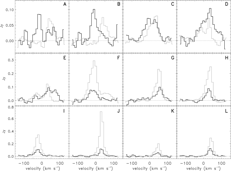
Figure 10: Spectra from NH₃(3,3) (grey) and NH₃(6,6) (black) at the positions labeled in Figure 9. For both transitions, we use image cubes deconvolved using a $14^{\prime\prime}$ Gaussian taper. Spectra are Hanning smoothed and the noise levels are $\sigma^{*}_{33,ch}=7.6$ mJy Beam^-1 and $\sigma^{*}_{66,ch}=9.5$ mJy Beam^-1.

Un-physical (6,6)-to-(3,3) line ratios (where $R_{m,63}>2.3$) are found throughout the central 2 pc. Figure 9 shows the positions of 12 spectra overlaid on velocity integrated NH₃(6,6) emission. Figure 10 plots the corresponding NH₃(3,3) (grey) and NH₃(6,6) (black) spectra. The spectra have been Hanning smoothed, and have an rms noise in one channel of 7.6 and 9.5 mJy for NH₃(3,3) and (6,6), respectively. Spectrum A is coincident with Sgr A*. In this section, we focus on the spectra associated with un-physical line ratios. Gas kinematics will be discussed in the following section.

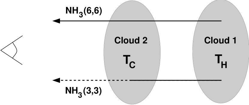
Figure 11: Schematic model of the orientation of a hot and cold cloud that can produce “un-physical” NH₃ (6,6)-to-(3,3) line ratios.

Un-physical NH₃ (6,6)-to-(3,3) line ratios occur near –20 km s^-1 in spectra A and B, and +70 km s^-1 in spectra D and E. These line ratios do not appear to result from an enhancement in NH₃(6,6) emission. Instead, they occur at velocities where there is no NH₃(3,3) emission. This complete lack of NH₃(3,3) emission implies that un-physical line ratios are likely the result of an absorption process along the LOS. The most straightforward scenario for the origin of un-physical line ratios is one in which emission from a hot cloud with a high (but physical) (6-6)-to-(3,3) line ratio, passes through cold molecular material along the line of sight. The lower-energy NH₃ (3,3) emission will be significantly absorbed by the cold cloud, while NH₃(6,6) will be relatively unaffected. This model is drawn schematically in Figure 11 and explored in more detail in the following paragraphs.

For simplicity, we assume that there is no radiative coupling between the two clouds in our model. From basic radiative transfer, the brightness temperature of the first cloud is expressed as

$$T_{b,1}=T_{ex,1}(1-e^{-\tau_{1}})+T_{bg}e^{-\tau_{1}}~{}.$$ (17)

For the cold cloud we assume that the background temperature is equal to the temperature of the CMB. If Cloud 2 is near Cloud 1, then emission from Cloud 1 will dominate the background, and the brightness temperature of the second cloud is

$$T_{b,2}=T_{ex,2}(1-e^{-\tau_{2}})+T_{b,1}e^{-\tau_{2}}~{}.$$ (18)

The antenna temperatures “on” and “off” source are related to the brightness temperature of Cloud 2 by

$$T_{A,{\rm on}} = \eta\left[\Phi T_{b,2}+(1-\Phi)T_{{\rm CMB}}\right]$$ (19)

$$T_{A,{\rm off}} = \eta T_{{\rm CMB}}~{},$$ (20)

where $\eta$ is the telescope efficiency and $\Phi$ is the filling factor of the source in the telescope beam. The difference between these two antenna temperatures will correspond to the measured antenna temperature due to the source ($\Delta T_{A}$). In practice, $\Delta T_{A}$ must be corrected for the fraction of emission in the main hyperfine component ($k$). For NH₃(3,3) and (6,6), however, the population of satellite hyperfine lines relative to the main component is very small and can be ignored ($k_{6}/k_{3}=1.08$). Assuming equal efficiencies and filling factors for NH₃(3,3) and (6,6), the observed main line ratio is therefore

$$R_{m,63}\approx\frac{\Delta T_{A}(6,6)}{\Delta T_{A}(3,3)}=\frac{T_{b,2}(6,6)-T_{{\rm CMB}}}{T_{b,2}(3,3)-T_{{\rm CMB}}}~{}.$$ (21)

In order to produce un-physical line ratios, Cloud 2 must have $\tau_{2}(3,3)\gg 1$ and $\tau_{2}(6,6)\ll 1$. This can be accomplished most efficiently for a cold cloud with $T_{C}\approx 30$ K. Kinetic temperatures $<30$ K have only minimal populations in both transitions, and although the relative population of NH₃(3,3) compared to NH₃(6,6) is higher at temperatures lower than 30 K, the small population of these transitions requires a large H₂ column density. Clouds with temperatures greater than 40 K will begin to have a significant population of NH₃(6,6) and both lines will be affected by absorption in the foreground cloud.

Assuming $\tau_{2}(3,3)\gg 1$, the brightness temperature of the second cloud will be approximately equal to $T_{ex,2}(3,3)$. For NH₃(6,6), however, $\tau_{2}(6,6)\ll 1$ implies that $T_{b,2}(6,6)\approx T_{b,1}(6,6)$. Therefore, the observed line ratio can be approximately written as

$$R_{m,63}\approx\frac{T_{b,1}(6,6)-T_{{\rm CMB}}}{T_{ex,2}(3,3)-T_{{\rm CMB}}}~{}.$$ (22)

Un-physical line ratios with $R_{m,63}\gg 1$ imply that $T_{b,1}(6,6)\gg T_{ex,2}(3,3)$. Assuming that the NH₃(6,6) excitation temperature in Cloud 1 exceeds $T_{{\rm CMB}}$, then Equation 16 implies that $T_{b,1}(6,6)\leq T_{ex,1}(6,6)$. Therefore, un-physical line ratios will generally imply that $T_{ex,1}(6,6)\gg T_{ex,2}(3,3)$. As seen in §3.2, such large differences in excitation temperatures imply that the H₂ density must exceed $10^{5}$ cm^-3 in these clouds (see Figure 4).

It should be noted that un-physical (6,6)-to-(3,3) line ratios were not reported in the survey of Galactic center molecular clouds by Armstrong & Barrett (1985). However, these data do not include any molecular gas within 2 pc of Sgr A* (see Figure 8d). In addition, the single-dish measurements have a resolution of only $84^{\prime\prime}$, and thus sample the average temperature structure on scales of $\sim 3$ pc. Clouds with high or un-physical line ratios are likely to be small and therefore fill only a fraction of the telescope beam. Cool gas, however, is prevalent throughout the entire region. The inclusion of significant amounts of cool gas within the telescope beam will lower the observed line ratios. Because our VLA data have a resolution of $16^{\prime\prime}\times 14^{\prime\prime}$, they are more sensitive to the temperature structure of molecular clouds on small scales. However, evidence for beam dilution of high line ratios is still detected at velocities near 20 km s^-1. Although some (6,6)-to-(3,3) line ratios greater than one occur near 20 km s^-1 (see Spectra C, D, and E), no line ratios exceed $\sim 2$. It is likely that any un-physical line ratios at these velocities are diluted by emission from cool gas in the 20 km s^-1 GMC. If beam dilution greatly affects observed line ratios, then the cloud that produces the un-physical line ratios must be significantly smaller than the synthesized beam of our VLA data.

It is also worth noting that the maximum allowed line ratio can exceed $1/C_{ul}$ if the cloud is not in LTE. Equation 14 assumes equal telescope efficiencies, filling factors, and excitation temperatures for the two transitions. If the values of these parameters for the upper transition exceed those for the lower transition, then the corresponding limit on the line ratio will exceed $1/C_{ul}$. However, because the energy separation of the inversion doublets is very small, it seems difficult to imagine a scenario in which the excitation temperatures of the two transitions differ significantly. We prefer the absorption model outlined above because it provides a simple explanation for un-physical line ratios that is consistent with observed spectral line profiles without having to invoke non-LTE conditions.

In summary, we believe that the un-physical line ratios observed to the east and southeast of Sgr A* are the result of absorption of NH₃(3,3) emission from a hot cloud near Sgr A* by cool material along the LOS. Although the current resolution of these data prevents a determination of the exact parameters of this cloud, the un-physical line ratios require that at least the hot material must be contained in a dense component with $n_{H_{2}}\lower 2.15277pt\hbox{$\;\buildrel>\over{\sim}\;$}10^{5}$ cm^-3.

6 Separating Multiple Gas Components Near Sgr A*

Spectra taken from the central 2 pc of the Galaxy are very complicated, with strong evidence for multiple clouds projected along the LOS (see spectra A–F in Figure 10). The (6,6)-to-(3,3) line ratios can be used to separate emission from the absorbed hot cloud from emission associated with cool, un-absorbed gas. Direct comparison of line ratios can be difficult because many features have infinite NH₃ (6,6)-to-(3,3) line ratios. We therefore separate these gas components by using the difference between the NH₃(3,3) and (6,6) emission. Gas with $S_{\nu}(6,6)>S_{\nu}(3,3)$ is termed “high line ratio” (HLR) gas, while gas with $S_{\nu}(6,6)<S_{\nu}(3,3)$ is called “low line ratio” (LLR) gas. This designation works well because gas with $S_{\nu}(6,6)=S_{\nu}(3,3)$ (or $R_{m,63}=1$) corresponds to a rotational temperature of 340 K, or a kinetic temperature of thousands of Kelvin. Because most NH₃ molecules will be destroyed at these temperatures, (6,6)-to-(3,3) line ratios greater than one most likely result from absorption of NH₃(3,3) emission from a hot cloud by cool intervening material.

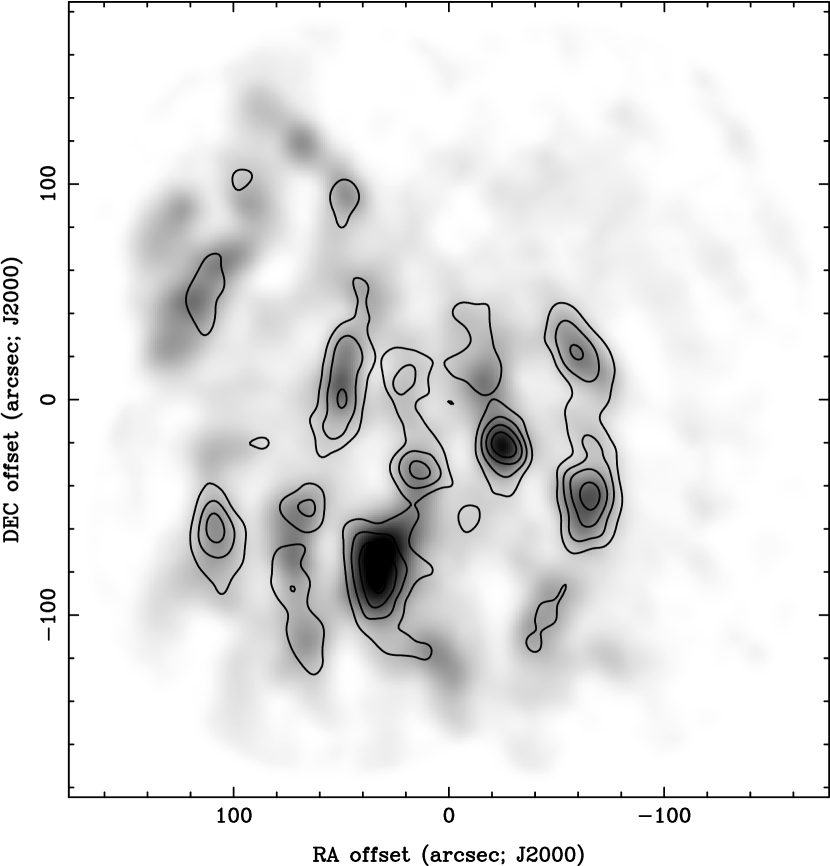
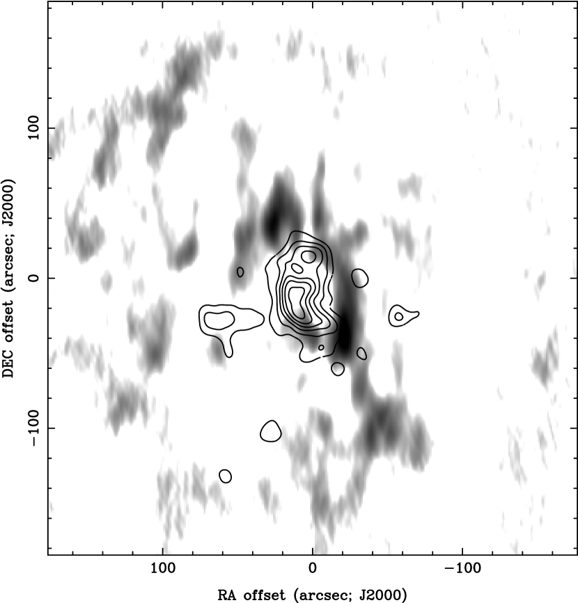
Figure 12: Left: Velocity integrated map of NH₃(6,6) emission at all points with NH₃ (6,6)-to-(3,3) line ratios less than one overlaid on a grey scale map of velocity integrated NH₃(3,3) emission. Contours are in steps of $3\sigma_{66}$ where $\sigma_{66}=0.33$ Jy Beam^-1 km s^-1. Low line ratio gas has a similar distribution to velocity integrated emission from lower-energy rotation inversion transitions. Right: Velocity integrated map of NH₃(6,6) emission at all points with NH₃ (6,6)-to-(3,3) line ratios greater than one overlaid on a grey scale map of velocity integrated HCN(1–0) emission (Wright et al., 2001). Contour levels are the same as in the left-hand panel. High-line-ratio (HLR) gas is confined to the inner 2 pc, interior to the CND, and a tongue of emission extending to the east at $\Delta\delta=-30^{\prime\prime}$.

The difference in NH₃(3,3) and (6,6) flux is calculated at every pixel ($x,y,v$) where the emission exceeds three sigma in at least one of the tracers. Figure 12 plots velocity integrated NH₃(6,6) emission associated with each gas component. The left-hand panel of Figure 12 plots velocity integrated map of NH₃(6,6) emission associated with the LLR component in contours overlaid on a velocity integrated map of NH₃(3,3) in grey scale. There is a very high degree of correspondence between the two maps, confirming that LLR gas traces clouds observed in lower rotation inversion transitions. Spectra F–L in Figure 10 show characteristic line profiles for LLR gas. The right-hand panel of Figure 12 overlays a velocity integrated map of NH₃(6,6) emission associated with HLR gas on a velocity integrated map of HCN(1–0) from Wright et al. (2001). HLR gas is predominantly located within 2 pc of the Galactic center and interior to the CND. A tongue of HLR gas also extends to the east of the nucleus ($60^{\prime\prime}$, $-30^{\prime\prime}$) with a velocity of 25 km s^-1. This HLR gas does not appear to be associated with the streamer at 60 km s^-1 and offset roughly $50^{\prime\prime}$ to the northeast of Sgr A* that was detected in HCN(1–0) by Ho (1995).

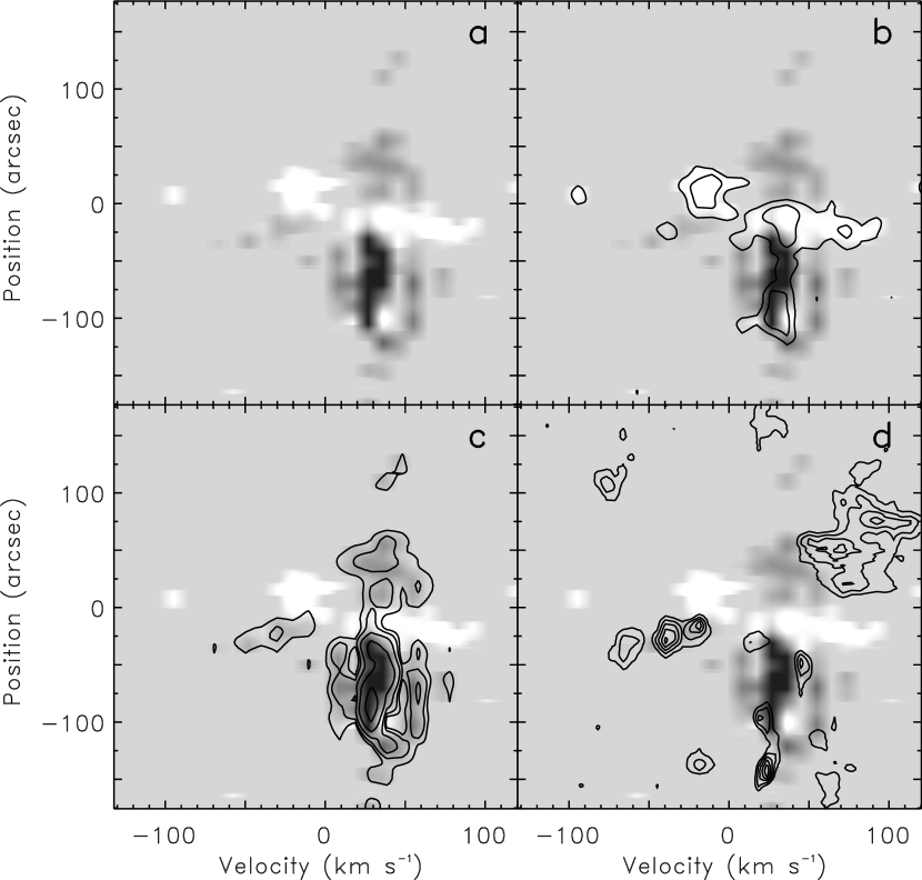
Figure 13: Position velocity diagrams showing the distribution of molecular gas in the central 2 pc. The position of the cut is labeled in Figure 9. A position of $0^{\prime\prime}$ corresponds to $\Delta\delta=0^{\prime\prime}$, and positive positions are to the northwest of Sgr A*. In all four panels, $S_{\nu}(6,6)-S_{\nu}(3,3)$ is plotted in grey scale. High-line-ratio gas ($S_{\nu}(6,6)>S_{\nu}(3,3)$) appears as white, while low-line-ratio gas ($S_{\nu}(6,6)<S_{\nu}(3,3)$) is dark grey. Although $S_{\nu}(6,6)-S_{\nu}(3,3)$ ranges between –0.65 and 0.13, the grey scale stretch ranges from –0.25 to 0.25 to highlight the different components in the data. b) NH₃(6,6) overlaid in contour steps of $3\sigma_{66,ch}$. NH₃(6,6) emission is observed from both the HLR and LLR gas. c) NH₃(3,3) overlaid in contour steps of 3, 6, 12, 24, and $48~{}\sigma_{33,ch}$. NH₃(3,3) emission comes only from LLR gas. d) HCN(1–0) from Wright et al. (2001) overlaid in contour steps of 0.25 Jy Beam^-1. The lack of HCN(1–0) emission at 30 km s^-1 is the result of self-absorption.

Figure 9 shows the location of a position-velocity cut that begins in the southern streamer and passes northwards through the central 2 pc of the Galaxy. The corresponding position velocity diagram of $S_{\nu}(6,6)-S_{\nu}(3,3)$ is shown in grey scale in Figure 13. Although $S_{\nu}(6,6)-S_{\nu}(3,3)$ ranges between –0.65 and 0.13, the grey scale stretch ranges from –0.25 to 0.25 to highlight the different components in the data. Black corresponds to LLR gas, and white corresponds to HLR gas. The $0^{\prime\prime}$ position corresponds to $\Delta\delta=0^{\prime\prime}$.

Panels $b-d$ of Figure 13 compare the difference map to emission from three molecular tracers. In Figure 13b, we overlay a position-velocity cut from our NH₃(6,6) data cube. Contours are in steps of $3\sigma_{66,ch}$, where $\sigma_{66,ch}=0.014$ Jy Beam^-1 (Herrnstein & Ho, 2002). Emission from NH₃(6,6) is present in both the HLR and LLR gas. Figure 13c plots a position-velocity cut of NH₃(3,3) with contours in steps of 3, 6, 12, 24, and $48\sigma_{33,ch}$, where $\sigma_{33,ch}=0.011$ Jy Beam^-1 (McGary et al., 2001). Unlike NH₃(6,6), NH₃(3,3) emission is only present in the LLR gas. The lack of NH₃(3,3) emission is consistent with all of the HLR gas resulting from absorption of NH₃(3,3) by cool intervening material along the LOS.

In Figure 13d, we plot a position-velocity diagram of HCN(1–0) from Wright et al. (2001). This position-velocity diagram resembles neither the NH₃(6,6) nor (3,3) plot. From $-150^{\prime\prime}$ to $-30^{\prime\prime}$, only the line wings of the southern streamer are detected. Self-absorption of HCN(1–0) is detected throughout the central 10 pc of the Galaxy (see spectra A, B, C, D, and F in Wright et al. (2001)) and strongly affects emission from the massive clouds (McGary et al., 2001). The strong self-absorption results from the low equivalent temperature of the HCN(1–0) transition (5 K). The higher equivalent temperatures of NH₃ (equal to $125$ K for NH₃(3,3)) make the rotation inversion transitions much less susceptible to absorption. Although not precisely coincident, the HCN(1–0) emission appears to be most closely related to emission from NH₃(3,3) and the LLR gas.

6.1 The Circumnuclear Disk

Faint NH₃(3,3) emission associated with the CND is detected at $-30$ km s^-1 at $-20^{\prime\prime}$ in Figure 13c. The CND is the dominant feature in the HCN(1–0) data, with emission observed from $-70$ km s^-1 at $-30^{\prime\prime}$ to $+100$ km s^-1 at $80^{\prime\prime}$ (see Figure 13d). However, the HCN(1–0) emission is not coincident with the NH₃(3,3) emission. In particular, HCN(1–0) emission at $-20^{\prime\prime}$ shows two peaks at $-20$ and $-40$ km s^-1 that bracket the NH₃(3,3) emission at $-30$ km s^-1, indicating that self-absorption of HCN(1–0) is a significant effect even in the CND.

It is well-established that there is a lack of HCN(1–0) emission in the southeastern part of the CND (Güsten et al., 1987; Wright et al., 2001). In Figure 13d, we find that emission from HCN(1–0) and HLR gas do not overlap at any position. Therefore, it might be suspected that the same material that absorbs NH₃(3,3) to produce un-physical (6,6)-to-(3,3) line ratios also absorbs HCN(1–0) emission from the eastern side of the CND. However, a detailed comparison of the HCN and NH₃ data in the “missing” southeastern part of the CND indicate that this scenario is unlikely. Both HCN(1–0) and HLR gas are absent at a position of ($40^{\prime\prime}$, $-10^{\prime\prime}$) relative to Sgr A* (see Figure 12). At ($25^{\prime\prime}$, $-20^{\prime\prime}$) HLR gas overlaps part of the missing ring, but it has velocities from $30-100$ km s^-1  and will not absorb emission from the CND, which is expected to have velocities between $\pm 20$ km s^-1(see Figure 12 of Wright et al. (2001)). Finally, lower line ratios near 20 km s^-1 indicate that the HLR gas cloud has a small filling factor compared to the southern streamer. It is thus unlikely that the cloud could absorb a significant portion of the CND. The “missing” southeastern part of the CND most likely reflects an intrinsically clumpy morphology.

6.2 The Southern Streamer

The majority of LLR gas in Figure 13 is associated with the southern streamer. This northeastern extension of the 20 km s^-1 GMC towards the CND has been suggested to be physically connected to the nucleus (Ho et al., 1991; Coil & Ho, 1999; McGary et al., 2001). However, this model has been hindered by a small velocity gradient and only minimal heating. For a central mass of $10^{7}~{}M_{\odot}$, a cloud at a distance of 5 pc should have a velocity gradient of $\sim 9$ km s^-1 pc^-1 (Coil & Ho, 1999). However, a velocity gradient of only 2–3 km s^-1 pc^-1 is measured along the 5 pc length of this cloud (Coil & Ho, 1999). The small observed velocity gradient implies that the bulk of the acceleration must occur perpendicular to the LOS. This orientation seems unlikely, however, because the 20 km s^-1 GMC is known to be located in front of the Galactic center along the LOS (see §7).

LLR gas associated with the southern streamer has a typical velocity of 20–30 km s^-1. Strong NH₃(3,3) emission is associated with this feature (see Figure 13c), and even the outer satellite hyperfine lines, which are offset by $\pm 29$ km s^-1 from the main line, are detected. Emission from the southern streamer appears to continue to the north of the CND, with no evidence for a significant change in velocity. LLR gas can also be seen in Spectrum A of Figure 10. In this spectrum, the LLR gas shows slightly higher velocities of $\sim 50$ km s^-1. This molecular gas at 50 km s^-1 is most likely responsible for the stimulated H 92$\alpha$ emission observed towards Sgr A* by Roberts & Goss (1993). Assuming that the LLR gas in Spectrum A is associated with the southern streamer, we measure an upper limit for the velocity gradient along the streamer of 12 km s^-1 arcmin^-1 (5 km s^-1 pc^-1), which is still a factor of two smaller than the expected gradient for infalling gas. Increased line widths near the CND were also reported by (Coil & Ho, 1999). In NH₃(3,3) we see no significant evidence for line width broadening associated with the LLR gas. Based on the continuation of the streamer to the north of Sgr A* as well as the lack of a large velocity gradient or increased line widths, we conclude that the southern streamer shows no conclusive evidence for direct interaction with material in the central 2 pc of the Galaxy. Instead, its apparent approach towards the Galactic center is most likely the result of projection along the LOS in front of Sgr A*.

Although we favor the above model for the southern streamer, the $15^{\prime\prime}$ resolution of our data prevents us from unequivocally ruling out an interaction of some type with the nucleus. While the kinematics of the southern streamer do not indicate a close association with the nucleus, it should be noted that a significant change in the NH₃(3,3) emission occurs at roughly the location of the southern lobe of the CND. NH₃(3,3) emission north of the CND is significantly weaker than the emission to the south. The coincidence of this change with the nucleus may indicate that there is some interaction between this cloud and the nucleus.

It is also possible that the faint LLR emission to the north of Sgr A* is not associated with the southern streamer at all. LLR emission from $0-50^{\prime\prime}$ in Figure 13c appears to fill in the velocities between the two lobes of high velocity emission associated with the CND. Continuous emission from $-30^{\prime\prime}$ to $+80^{\prime\prime}$ would imply that the CND extends very close to the nucleus, which is contrary to the current model of the CND as a ring-like structure. However, observations of HCN(1–0) emission from the CND have shown that it is warped and clumpy, and it differs significantly from a simple Keplerian ring (Güsten et al., 1987). It has even been suggested that the structure is the result of three independent clouds in orbit about the nucleus (Wright et al., 2001). A more precise understanding of the CND is necessary to rule out an association with the 30 km s^-1 LLR gas to the north of Sgr A*.

Finally, the faint NH₃(3,3) emission to the north of Sgr A* may partially result from “blooming” of flux during the MEM deconvolution. (Blooming occurs when extra flux in the form of a faint, extended component is added to the image by MEM in order to obtain the “best” solution.) Because emission to the north of the CND has slightly more red-shifted velocities than the bright southern emission, we believe that it is unlikely that this emission is the result of blooming. These questions should be resolved with the future addition of single-dish data, which will eliminate deconvolution artifacts and also allow us to use the full $3^{\prime\prime}$ resolution of the data.

6.3 The High-Line-Ratio Cloud

High line ratio gas has a very different kinematic structure from the southern streamer and CND. Figure 13 shows that HLR gas has a large velocity gradient from $\lower 2.15277pt\hbox{$\;\buildrel>\over{\sim}\;$}50$ km s^-1 at $-20^{\prime\prime}$ to –20 km s^-1 at $\sim 0^{\prime\prime}$ and then back to 0 km s^-1 at $+20^{\prime\prime}$. Due to the large range of velocities over which HLR gas is observed, a cool gas cloud along the LOS cannot produce the majority of the absorption of NH₃(3,3). The absorbing material responsible for the un-physical (6,6)-to-(3,3) line ratios most likely lies in a shielded outer layer of the same cloud. The rotation of the HLR cloud is in the opposite sense as the CND. The gradient is in the same direction as the high velocity cloud discussed in McGary et al. (2001), but the positions and velocities of the emission from the two features do not precisely agree. Improved spatial resolution is necessary to determine the exact morphology of this cloud.

The large velocity gradient in the HLR gas explains the observed line widths of of 80–90 km s^-1 in Figure 2 of Herrnstein & Ho (2002). The true line width of the gas can be measured at the turning point in the NH₃(6,6) position-velocity diagram (position of $0^{\prime\prime}$ in Figure 13b). We estimate that the intrinsic line width of the HLR gas is $\sim 20$ km s^-1. This line width is very similar to intrinsic line widths determined for the other molecular features in the central 10 pc (see Figure 2c).

Line ratios at the position where HLR gas crosses the 20 km s^-1 GMC favor a model in which the HLR cloud is significantly smaller than the synthesized beam of these data. At a position of $-15^{\prime\prime}$ in Figure 13a, there is a slight decrease in the values of $S_{\nu}(6,6)-S_{\nu}(3,3)$. Lower (6,6)-to-(3,3) line ratios are consistent with beam dilution of line ratios at these velocities by cool emission from the southern streamer.

The “hook” profile of the position-velocity diagram for the HLR gas is characteristic of a cloud that is undergoing both rotation and either infall or expansion (Keto et al., 1988). The position-velocity profile of the HLR gas is best fit by a linear velocity gradient of –1.6 km s^-1 arcsec^-1 ($-40$ km s^-1 pc^-1) and expansion or contraction at 80 km s^-1. Assuming the gradient is due to circular rotation and that the measured length of the cloud ($\sim 1$ pc) is twice the radius, the observed gradient corresponds to rotation at 20 km s^-1. This rotation velocity implies a minimum enclosed mass of $4\times 10^{4}$ $M_{\odot}$. If the cloud is assumed to have a circular orbit around a mass of $10^{7}$ $M_{\odot}$, then the observed velocity gradient would correspond to an inclination of $\sim 4^{\circ}$. Such a low inclination is unlikely, although it cannot be ruled out with the current resolution, and the HLR cloud is probably not in a circular orbit.

Because emission is blue-shifted from the expected rotation velocities, we must either be observing emission from the far side of a contracting cloud or the near side of an expanding shell. We currently favor a model in which we are observing the near edge of an expanding shell. Assuming the source of the expansion is therefore behind the observed shell along the line-of-sight, then it naturally follows that the cool layer which absorbs the NH₃(3,3) would be located between the hot material on the inner edge of the shell and the observer. Although it is possible that the other half of the shell is truly missing, the lack of symmetry may also provide clues to the morphology of the shell and the location of the cool absorbing material. Improved spatial resolution will be useful in resolving this question.

7 Towards a 3-D Model of the Central 10 pc

In the preceding sections, we have investigated the physical conditions and interactions of dense molecular clouds within 5 pc of Sgr A*. We briefly summarize our main results below:

• The 50 km s^-1 GMC shows no evidence for a strong interaction with Sgr A East. Based on the observed effects of Sgr A East on the western streamer, we find that the energy of Sgr A East is consistent with a single supernova occurring roughly $10^{4}$ years ago (§4).

• The temperature structure of dense clouds in the central 10 pc can be characterized by a two-temperature structure on scales of 0.5 pc. The data are consistent with the structure on scales of 3 pc proposed by (Hüttemeister et al., 1993a), in which roughly one quarter of the gas is in a hot component at 200 K.

• NH₃ (6,6)-to-(3,3) line ratios in the central 2 pc exceed theoretical limits for gas in LTE (§5.2). We conclude that these line ratios result from absorption of NH₃(3,3) by a cool, shielded layer of the same cloud. This result implies that $n_{H_{2}}\lower 2.15277pt\hbox{$\;\buildrel>\over{\sim}\;$}10^{5}$ cm^-3.

• Three distinct molecular gas components lie within a projected distance of 2 pc from Sgr A* (§6). Both the CND and the “high-line-ratio gas” show large velocity gradients, although in opposite directions. Emission associated with the southern streamer, however, shows no significant velocity gradient, and extends to the north of the nucleus.

It is important to relate the molecular features described in this paper to other structures in the nuclear region. Discussions of the central parsecs of the Galaxy seem to inevitably evolve into discussions of the location of these structures along the LOS. In this concluding section, we present a model for the LOS arrangement of the features in the central 10 pc. The model is based on the molecular line data presented in this paper as well as the most current results in the published literature. The model is not to scale (or completely inclusive), but it is presented to promote discussion of the interaction between different structures observed at the Galactic center.

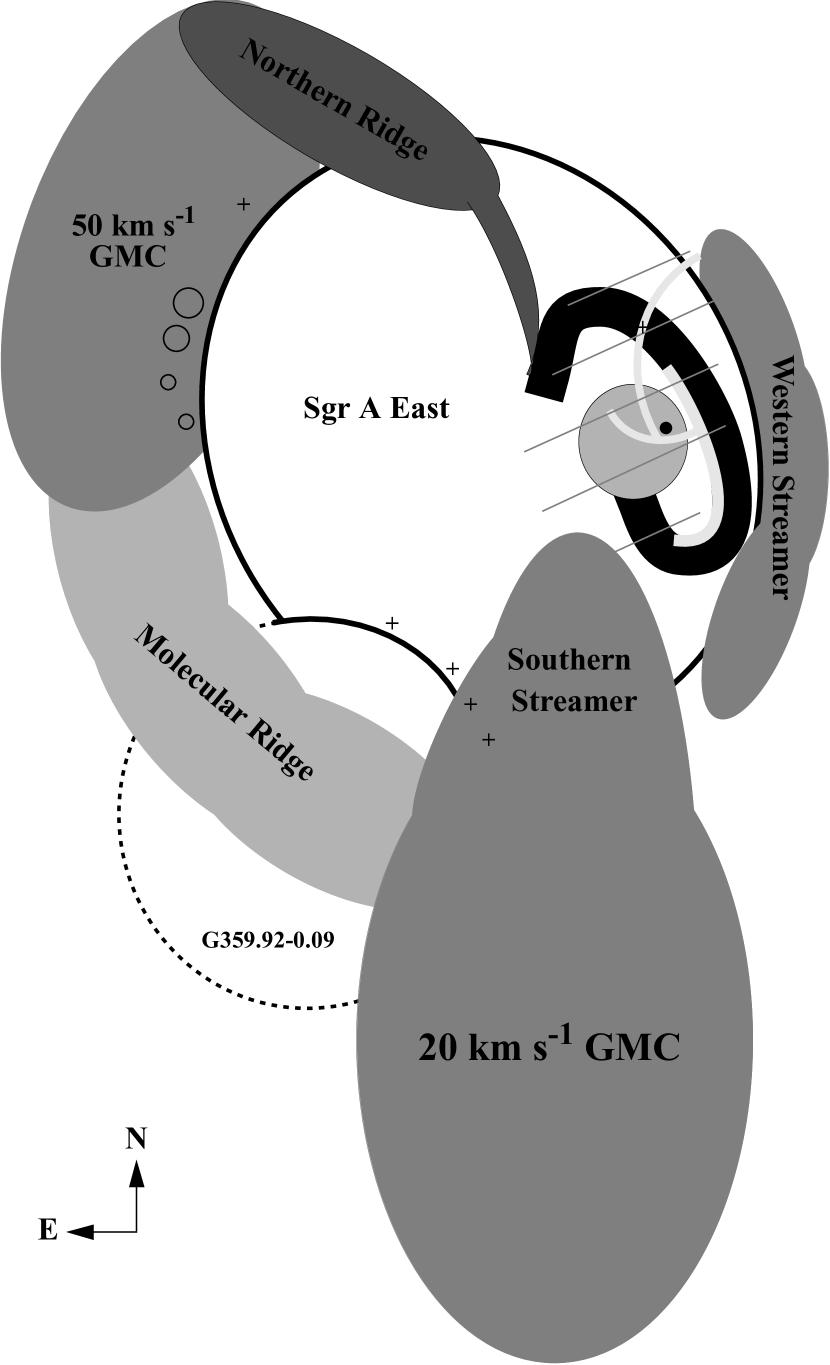
Figure 14: Schematic drawing of the Galactic center as seen in the plane of the sky.

A schematic drawing of the main structures in the central 10 pc of the Galaxy is presented in Figure 14. The elongated Sgr A East shell fills the center of the image. Towards the western side of the shell, a black dot shows the location of Sgr A*, which is surrounded by the arcs of Sgr A West (light grey) and the backwards “C” shape of the CND (black). The cloud of HLR gas discussed in §6 is also shown in close proximity to Sgr A*. Because its exact morphology is not known, it is shown as a grey circle, slightly offset to the southeast of Sgr A*. The major molecular features described in this paper are labeled. Hatched lines extending northwards from the southern streamer indicate the faint extension of this cloud to the north of Sgr A* (see §6.2). A second supernova, G359.92–0.09, which is impacting Sgr A East in the southeast is also shown (Coil & Ho, 2000). Positions of 1720 MHz OH masers (Yusef-Zadeh et al., 1999) are marked with crosses, and the Hii regions observable at 6 cm are shown as small circles in the 50 km s^-1 GMC.

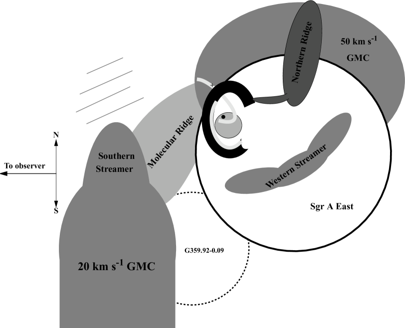
Figure 15: Schematic drawing of the Galactic center with left denoting the direction to the observer and the vertical direction denoting north and south.

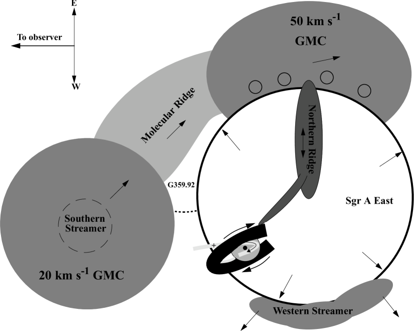
Figure 16: Schematic drawing of the Galactic center with left denoting the direction to the observer and the vertical direction denoting east and west. Arrows show the inferred motions of the main features based on the Doppler-shifted velocities.

In Figures 15 and 16, we present schematic drawings of the proposed location of these structures along the LOS. Figure 16 also shows the motions of the clouds inferred from their Doppler-shifted velocities. The LOS structure of the arcs of Sgr A West is based on H 92$\alpha$ emission from Roberts & Goss (1993). Because the location of the eastern bar relative to Sgr A* is not well known, it is not included in the LOS model. The northern arc is best described as a tidally disrupted cloud that is passing within 0.13 pc of Sgr A*. The orbit produces high negative velocities of –250 km s^-1 at the southern-most end of the arc (Roberts & Goss, 1993; Roberts et al., 1996). The western arc, however, is coincident with the inner edge of the circumnuclear disk, and most likely is the ionized inner layer of this structure (Roberts & Goss, 1993). Absorption of starlight and Br$\gamma$ emission from the western arc of Sgr A West favors an orientation of the CND with the western side in front of the Galactic center along the LOS (Roberts & Goss, 1993). The location of the HLR molecular gas is schematically drawn interior to the CND, but exact determination of the morphology and location of this cloud cannot be determined with the current resolution of our data.

Absorption of 90 cm continuum emission from Sgr A East by Sgr A West places the nucleus in front or just inside Sgr A East (Pedlar et al., 1989). The connection of the northern ridge, which lies along the northern edge of Sgr A East, to the CND indicates that Sgr A East must be within a few parsecs of the nucleus (McGary et al., 2001). More recently, Maeda et al. (2002) place Sgr A*, Sgr A West, and the CND just inside the leading edge of Sgr A East. (For schematic drawings of proposed relative locations of Sgr A West, Sgr A*, and Sgr A East, see e.g. Pedlar et al. (1989) and Maeda et al. (2002).)

As discussed in §4, the velocity gradient of the western streamer indicates that it is highly inclined to the LOS and expanding outwards with Sgr A East. The northern ridge is placed along the northern edge of Sgr A East. The cloud is located at the same distance as the center of Sgr A East, with an orientation roughly in the plane of the sky. This placement allows for the bulk of the motion associated with the expansion of Sgr A East to occur perpendicular to the line of sight, consistent with its velocity of –10 km s^-1.

The 50 km s^-1 cloud is located predominately to the east of Sgr A East. As discussed in §6, stimulated H 92$\alpha$ emission at 50 km s^-1 observed towards Sgr A* (Roberts & Goss, 1993) is most likely associated with the southern streamer and not the GMC. The 50 km s^-1 cloud is not observed to strongly absorb X-ray emission from the central 10 pc (Park et al., 2004), which also implies that little of the material is in front of the Galactic center along the LOS. This GMC is connected to the 20 km s^-1 cloud along the molecular ridge (Coil & Ho, 2000). As mentioned in §4, the Hii regions found along the interior of the western edge of this GMC are much too old to have been caused by the current impact of Sgr A East.

Observations of formaldehyde absorption towards the Galactic center, indicate that the 20 km s^-1 GMC lies in front of the nucleus along the LOS (Güsten & Downes, 1980). This placement has been recently confirmed by absorption of 2–10 keV X-rays in the region of this GMC (Park et al., 2004). The distance between the 20 km s^-1 GMC and the nucleus is constrained by observations of SNR 359.92–0.09. This SNR was first reported by Coil & Ho (2000), who detected it in 20 cm radio continuum images from Yusef-Zadeh & Morris (1987). More recently, an X-ray filament associated with the southwest edge of this SNR has been detected with both XMM-Newton and Chandra (Sakano et al., 2003; Park et al., 2004). The impact of SNR 359.92–0.09 is responsible for the concave morphology of Sgr A East in the southeast. Multiple 1720 MHz OH masers with velocities of $\sim 50$ km s^-1 have been detected along this interface region (Yusef-Zadeh et al., 1999). These masers have been associated with disrupted gas associated with the 20 km s^-1 GMC (Coil & Ho, 2000). Because SNR 359.92–0.09 is interacting with both Sgr A East and the 20 km s^-1 GMC, the GMC must be no more than $5-10$ pc from Sgr A*. Finally, based on the results of §6, the southern streamer is depicted as extending northwards from the 20 km s^-1 cloud, but not interacting with the nucleus.

Although uncertainties in this model undoubtedly remain, the fact that such a detailed three dimensional model of the Galactic center can be proposed based on observational data reflects the great advances in recent years in our understanding of this region. In particular, the data presented in this paper have shed new light on the role of dense molecular gas in the region around the supermassive black hole. The large velocity coverage of our VLA data combined with the relatively high excitation requirements of the rotation inversion transitions have resulted in a more complete picture of the location of dense material within 5 pc of Sgr A*. The additional knowledge of temperatures, line widths, and cloud masses, all of which are directly obtained from the NH₃ data, have enabled us to more precisely determine the interactions between these dense molecular clouds and other features near the nucleus. At present, a more precise understanding of the role of the dense molecular structures in the Galactic center is primarily hindered by the relatively low resolution ($16^{\prime\prime}\times 14^{\prime\prime}$) of our data. Future incorporation of measurements made with large single-dish telescopes should allow us to resolve many of the outstanding questions regarding dense molecular gas at the center of the Galaxy.

Table 1: Physical Parameters for Galactic Center Clouds

Parameter	Unit	Southern	Northern	SE1	SE2	Northern	50 km s-1	Western
		Streamer	Fork			Ridge	GMC	Streamer
Extent in R.A.	′′	–30, 60	–70, –30	60, 90	90, 140	30, 100	80, 150	–100, –40
Extent in Dec.	′′	–30, -150	–150, -90	–30, –140	–10, –100	80, 130	0, 125	–100, 100
$\langle\Delta{\rm v}_{{\rm int}}\rangle$	km s-1	15.2	13.9	14.6	16.7	15.8	16.9	20.5
$\sigma(\Delta{\rm v}_{{\rm int}})$	km s-1	8.1	5.4	8.1	10.0	4.0	6.4	4.5
$\langle\tau_{m}(1,1)\rangle$	…	2.4	3.0	2.2	1.9	0.5	2.5	0.4
$\sigma(\tau_{m}(1,1))$	…	0.7	0.2	0.7	0.3	0.4	0.5	0.3
$\langle T_{R21}\rangle$	K	26.4	25.4	28.9	29.3	28.2	21.4	30.9
$\sigma(T_{R21})$	K	5.1	2.8	5.2	4.7	4.5	2.9	3.9
$\langle T_{K}\rangle$	K	33	32	39	40	37	25	46
$\langle T_{ex}\rangle$	K	6.2	4.3	4.9	4.7	4.9	4.4	4.1
$\sigma(T_{ex})$	K	1.1	0.2	0.5	0.6	1.4	0.5	0.7
$\langle N_{(1,1)}\rangle$	$10^{15}$ cm-2	3.5	3.6	1.5	1.2	0.9	2.8	1.4
$\sigma(N_{(1,1)})$	$10^{15}$ cm-2	1.9	1.0	1.1	0.9	0.2	1.1	0.6
$\langle N_{{\rm NH_{3}}}\rangle$	$10^{15}$ cm-2	8.7	5.0	3.0	2.9	2.1	6.1	3.7
$\sigma(N_{{\rm NH_{3}}})$	$10^{15}$ cm-2	4.3	4.2	2.1	2.1	0.5	2.6	1.4
Area	$10^{3}\Box^{\prime\prime}$	4.0	0.3	1.5	2.2	0.4	3.3	0.4
Mass	$M_{\odot}$	$8\times 10^{4}$	$4\times 10^{3}$	1$\times 10^{4}$	$2\times 10^{4}$	$2\times 10^{3}$	$5\times 10^{4}$	$4\times 10^{3}$

Table 2: Summary of NH₃ Observations at the Galactic Center

Label	Telescope	Beam (′′)	Measured Temperatures	Reference
G81	Effelsberg	40	$T_{R21}$, $T_{R41}$, $T_{R42}$	Güsten et al. (1981)
O89	NMA	$24\times 13$	$T_{R21}$	Okumura et al. (1989)
A85	Haystack	84	$T_{R21}$, $T_{R63}$	Armstrong & Barrett (1985)
H93	NRAO 40-m	84	$T_{R21}$, $T_{R54}$	Hüttemeister et al. (1993a)
C99/00	VLA	$14\times 9$	$T_{R21}$	Coil & Ho (1999, 2000)
H04	VLA	$15\times 13$	$T_{R21}$	this paper

Table 3: NH₃ Rotational Temperature Measurements for Galactic Center Molecular Clouds

$\Delta\alpha$	$\Delta\delta$	$T_{R21}$	$T_{R41}$	$T_{R42}$	$T_{R54}$	$T_{R63}$	Ref.
(′′)	(′′)	(K)	(K)	(K)	(K)	(K)
$185$	$113$	…	$>47$	…	…	…	G81
$76$	$95$	…	$>44$	$>41$	…	…	G81
$143$	$53$	…	$>52$	$>54$	…	…	G81
$152$	$47$	…	$>49$	$>56$	…	…	G81
$177$	$32$	…	$>39$	$>43$	…	…	G81
$122$	$19$	…	$>49$	$>61$	…	…	G81
$62$	$-155$	66	46	46	…	…	G81
$30$	$-207$	…	…	49	…	…	G81
$-3$	$-259$	$55^{+15}_{-10}$	$45^{+15}_{-10}$	$49^{+10}_{-6}$	…	…	G81
$-67$	$-287$	96	47	43	…	…	G81
$-33$	$-308$	$100^{+51}_{-25}$	$40^{+4}_{-3}$	$37^{+6}_{-4}$	…	…	G81
$-66$	$-360$	71	46	43	…	…	G81
$-13$	$-392$	63	44	46	…	…	G81
$-97$	$-412$	91	40	37	…	…	G81
$39$	$-424$	51	41	46	…	…	G81
$219$	$100$	…	…	…	…	80 $\pm$ 16	A85
$94$	$70$	…	…	…	…	80 $\pm$ 16	A85
$172$	$23$	34 $\pm$ 7	…	…	…	75 $\pm$ 15	A85
$125$	$-54$	37 $\pm$ 7	…	…	…	75 $\pm$ 15	A85
$77$	$-130$	36 $\pm$ 7	…	…	…	100 $\pm$ 20	A85
$30$	$-207$	48 $\pm$ 10	…	…	…	80 $\pm$ 16	A85
$-18$	$-283$	31 $\pm$ 6	…	…	…	70 $\pm$ 14	A85
$59$	$-331$	…	…	…	…	100 $\pm$ 20	A85
$-66$	$-360$	62 $\pm$ 8	…	…	…	70 $\pm$ 14	A85
$-113$	$-436$	…	…	…	…	90 $\pm$ 18	A85
$-8$	$-203$	25 $\pm$ 7	…	…	…	…	O89
$-38$	$-203$	24 $\pm$ 5	…	…	…	…	O89
$-18$	$-233$	31 $\pm$ 7	…	…	…	…	O89
$-49$	$-253$	30 $\pm$ 13	…	…	…	…	O89
$-77$	$-253$	22 $\pm$ 25	…	…	…	…	O89
$-18$	$-263$	24 $\pm$ 3	…	…	…	…	O89
$-28$	$-263$	17 $\pm$ 2	…	…	…	…	O89
$-70$	$-263$	27 $\pm$ 34	…	…	…	…	O89
$-58$	$-323$	18 $\pm$ 3	…	…	…	…	O89
$-107$	$-323$	3 $\pm$ 6	…	…	…	…	O89
$-91$	$-347$	18 $\pm$ 3	…	…	…	…	O89
$-49$	$-353$	13 $\pm$ 3	…	…	…	…	O89
$-106$	$-335$	35 $\pm$ 2	…	…	$64\pm 4$	…	H93
$26$	$-23$	$32_{-5}^{+30}$	…	…	…	…	C99
$26$	$-83$	$22_{-5}^{+30}$	…	…	…	…	C99
$-13$	$-163$	$22_{-5}^{+30}$	…	…	…	…	C99
$144$	$4$	$20_{-5}^{+30}$	…	…	…	…	C00
$105$	$-126$	$30_{-5}^{+30}$	…	…	…	…	C00

Figure 2: NOTE: Image too large for astro-ph. Please download a full version of this paper at http://www.astro.columbia.edu/$\sim$herrnstein/NH3/paper/ .a) Mean value of NH₃(1,1) main line opacity ($\tau_{\rm{m}}(1,1)$). Contours are in integer steps. b) Significance of opacity determinations. Contours are 1, 2, 3, 6, 9, and 12$\sigma$. Hatches denote pixels for which only a lower limit for $\tau_{\rm{m}}(1,1)$ could be determined. c) Mean value of intrinsic line width ($\Delta\rm{v}_{int}$). Typical intrinsic line widths are 15 km s^-1. d) Significance of intrinsic line width determinations. Contours are in steps of $3\sigma$. Hatches denote pixels for which only an upper limit for $\Delta\rm{v}_{int}$ could be determined.

Figure 3: NOTE: Image too large for astro-ph. Please download a full version of this paper at http://www.astro.columbia.edu/$\sim$herrnstein/NH3/paper/ . a) Pseudo-color map of the derived (2,2)-to-(1,1) rotational temperature. Contours are in steps of 10 K. b) Significance of $T_{R21}$ determinations. Contours are in steps of 3$\sigma$. c) Derived values for the excitation temperature. Contours are in steps of 4 K. Compared to the rotational temperature, the excitation temperature is smoothly distributed (especially in regions with high S/N) with values between 4 and 8 K. d) Significance of the $T_{ex}$ values. Contours are 3, 15, 30, and 45$\sigma$.

Figure 4: Excitation temperature as a function of H₂ density for kinetic temperatures of 10, 30, 100, and 300 K. This plot is valid for NH₃(1,1), (2,2), (3,3), and (6,6) because the critical densities for these transitions are all equal to $2\times 10^{3}$ cm^-3. Gas is not thermalized until $n(H_{2})\approx 10^{6}$ cm^-3.

Figure 5: NOTE: Image too large for astro-ph. Please download a full version of this paper at http://www.astro.columbia.edu/$\sim$herrnstein/NH3/paper/ . Total column density of NH₃. Contours are in steps of $4\times 10^{15}$ cm^-2. Significance of $N_{{\rm NH_{3}}}$ determinations. Contours are in steps of 1.5$\sigma$.

Figure 6: Calculated kinetic temperature for $T_{R21}$, $T_{R42}$, $T_{R54}$, and $T_{R63}$ for six different combinations of hot gas at 200 K and cold gas at 15 K. a) Weighted mean kinetic temperatures calculated from the $T_{R21}$ and $T_{R63}$ measurements presented in this paper are overlaid as squares. b) Weighted mean kinetic temperatures calculated from published $T_{R21}$, $T_{R42}$, and $T_{R63}$ measurements in Figure 8 are overlaid as filled circles. The measurements of $T_{R21}$ and $T_{R54}$ from Hüttemeister et al. (1993a) are overlaid as triangles.

Figure 7: NOTE: Image too large for astro-ph. Please download a full version of this paper at http://www.astro.columbia.edu/$\sim$herrnstein/NH3/paper/ . a) Position of the single dish measurements listed in Table 3 overlaid on a grey scale image of 1.2 mm emission (Zylka et al., 1998). Contours denote 10, 20, 40, and 80% of the peak flux. Labels correspond to the list of observations in Table 2. b) Position of interferometric observations in the same region. Primary beams of the interferometer are plotted. For Okumura et al. (1989), the synthesized beam of the NMA is also overlaid at the positions where temperature measurements were made.

References

- Armstrong & Barrett (1985) Armstrong, J. T. & Barrett, A. H. 1985, ApJS, 57, 535
- Balick & Brown (1974) Balick, B. & Brown, R. L. 1974, ApJ, 194, 265
- Batrla et al. (1984) Batrla, W., Walmsley, C. M., & Wilson, T. L. 1984, A&A, 136, 127
- Benson & Myers (1983) Benson, P. J. & Myers, P. C. 1983, ApJ, 270, 589
- Coil & Ho (1999) Coil, A. L. & Ho, P. T. P. 1999, ApJ, 513, 752
- Coil & Ho (2000) —. 2000, ApJ, 533, 245
- Danby et al. (1988) Danby, G., Flower, D. R., Valiron, P., Schilke, P., & Walmsley, C. M. 1988, MNRAS, 235, 229
- Dent et al. (1993) Dent, W. R. F., Matthews, H. E., Wade, R., & Duncan, W. D. 1993, ApJ, 410, 650
- Ekers et al. (1983) Ekers, R. D., van Gorkom, J. H., Schwarz, U. J., & Goss, W. M. 1983, A&A, 122, 143
- Genzel et al. (1990) Genzel, R., Stacey, G. J., Harris, A. I., Townes, C. H., Geis, N., Graf, U. U., Poglitsch, A., & Stutzki, J. 1990, ApJ, 356, 160
- Ghez et al. (2003) Ghez, A. M., Becklin, E., Duchêne, G., Hornstein, S., Morris, M., Salim, S., & Tanner, A. 2003, in Astron. Nachr., Vol. 324, No. S1, Special Supplement “The central 300 parsecs of the Milky Way”, Eds. A. Cotera, H. Falcke, T. R. Geballe, S. Markoff,, Vol. 324, 527–533
- Green et al. (1997) Green, A. J., Frail, D. A., Goss, W. M., & Otrupcek, R. 1997, AJ, 114, 2058
- Güsten & Downes (1980) Güsten, R. & Downes, D. 1980, A&A, 87, 6
- Güsten et al. (1987) Güsten, R., Genzel, R., Wright, M. C. H., Jaffe, D. T., Stutzki, J., & Harris, A. I. 1987, ApJ, 318, 124
- Güsten et al. (1981) Güsten, R., Walmsley, C. M., & Pauls, T. 1981, A&A, 103, 197
- Herrnstein (2003) Herrnstein, R. M. 2003, Ph.D. Thesis
- Herrnstein & Ho (2002) Herrnstein, R. M. & Ho, P. T. P. 2002, ApJ, 579, L83
- Herrnstein & Ho (2003) —. 2003, Astronomische Nachrichten Supplement, 324, 583
- Ho (1995) Ho, P. T. P. 1995, in The Physics and Chemistry of Interstellar Molecular Clouds, Proceedings of the 2nd Cologne-Zermatt Symposium, Held at Zermatt, Switzerland, 21 - 24 September 1993. Edited by G. Winnewisser and G. C. Pelz. (Springer-Verlag: New York), 33
- Ho et al. (1991) Ho, P. T. P., Ho, L. C., Szczepanski, J. C., Jackson, J. M., & Armstrong, J. T. 1991, Nature, 350, 309
- Ho et al. (1977) Ho, P. T. P., Martin, R. N., Myers, P. C., & Barrett, A. H. 1977, ApJ, 215, L29
- Ho & Townes (1983) Ho, P. T. P. & Townes, C. H. 1983, ARA&A, 21, 239
- Hüttemeister et al. (1993a) Hüttemeister, S., Wilson, T. L., Bania, T. M., & Martin-Pintado, J. 1993a, A&A, 280, 255
- Hüttemeister et al. (1993b) Hüttemeister, S., Wilson, T. L., Henkel, C., & Mauersberger, R. 1993b, A&A, 276, 445
- Keto et al. (1988) Keto, E. R., Ho, P. T. P., & Haschick, A. D. 1988, ApJ, 324, 920
- Khokhlov & Melia (1996) Khokhlov, A. & Melia, F. 1996, ApJ, 457, L61+
- Lo & Claussen (1983) Lo, K. Y. & Claussen, M. J. 1983, Nature, 306, 647
- MacLaren et al. (1988) MacLaren, I., Richardson, K. M., & Wolfendale, A. W. 1988, ApJ, 333, 821
- Maeda et al. (2002) Maeda, Y. et al. 2002, ApJ, 570, 671
- Marshall et al. (1995) Marshall, J., Lasenby, A. N., & Harris, A. I. 1995, MNRAS, 277, 594
- Martin et al. (1982) Martin, R. N., Ruf, K., & Ho, P. T. P. 1982, Nature, 296, 632
- McGary et al. (2001) McGary, R. S., Coil, A. L., & Ho, P. T. P. 2001, ApJ, 559, 326
- McGary & Ho (2002) McGary, R. S. & Ho, P. T. P. 2002, ApJ, 577, 757
- Mezger et al. (1989) Mezger, P. G., Zylka, R., Salter, C. J., Wink, J. E., Chini, R., Kreysa, E., & Tuffs, R. 1989, A&A, 209, 337
- Morris & Serabyn (1996) Morris, M. & Serabyn, E. 1996, ARA&A, 34, 645
- Narayan et al. (1998) Narayan, R., Mahadevan, R., Grindlay, J. E., Popham, R. G., & Gammie, C. 1998, ApJ, 492, 554
- Okumura et al. (1989) Okumura, S. K. et al. 1989, ApJ, 347, 240
- Park et al. (2004) Park, S., Muno, M. P., Baganoff, F. K., Maeda, Y., Morris, M., Howard, C., Bautz, M. W., & Garmire, G. P. 2004, ApJ, 603, 548
- Pauls et al. (1983) Pauls, A., Wilson, T. L., Bieging, J. H., & Martin, R. N. 1983, A&A, 124, 23
- Pedlar et al. (1989) Pedlar, A., Anantharamaiah, K. R., Ekers, R. D., Goss, W. M., van Gorkom, J. H., Schwarz, U. J., & Zhao, J. 1989, ApJ, 342, 769
- Pierce-Price et al. (2000) Pierce-Price, D. et al. 2000, ApJ, 545, L121
- Quataert (2003) Quataert, E. 2003, Astronomische Nachrichten Supplement, 324, 435
- Reid (1993) Reid, M. J. 1993, ARA&A, 31, 345
- Reid & Brunthaler (2004) Reid, M. J. & Brunthaler, A. 2004, astro-ph/0408107
- Roberts & Goss (1993) Roberts, D. A. & Goss, W. M. 1993, ApJS, 86, 133
- Roberts et al. (1996) Roberts, D. A., Yusef-Zadeh, F., & Goss, W. M. 1996, ApJ, 459, 627
- Sakano et al. (2003) Sakano, M., Warwick, R. S., Decourchelle, A., & Predehl, P. 2003, MNRAS, 340, 747
- Schödel et al. (2002) Schödel, R. et al. 2002, Nature, 419, 694
- Serabyn & Guesten (1986) Serabyn, E. & Guesten, R. 1986, A&A, 161, 334
- Serabyn et al. (1992) Serabyn, E., Lacy, J. H., & Achtermann, J. M. 1992, ApJ, 395, 166
- Shull (1980) Shull, J. M. 1980, ApJ, 237, 769
- Stutzki & Winnewisser (1985) Stutzki, J. & Winnewisser, G. 1985, A&A, 148, 254
- Townes & Schawlow (1975) Townes, C. H. & Schawlow, A. L. 1975, Microwave Spectroscopy (New York: Dover Publications, Inc.)
- Uchida et al. (1998) Uchida, K. I., Morris, M., Serabyn, E., Fong, D., & Meseroll, T. 1998, in IAU Symp. 184: The Central Regions of the Galaxy and Galaxies, ed. Sofue, Y., 317
- Walmsley et al. (1987) Walmsley, C. M., Hermsen, W., Henkel, C., Mauersberger, R., & Wilson, T. L. 1987, A&A, 172, 311
- Walmsley & Ungerechts (1983) Walmsley, C. M. & Ungerechts, H. 1983, A&A, 122, 164
- Wright et al. (2001) Wright, M. C. H., Coil, A. L., McGary, R. S., Ho, P. T. P., & Harris, A. I. 2001, ApJ, 551, 254
- Yuan et al. (2002) Yuan, F., Markoff, S., & Falcke, H. 2002, A&A, 383, 854
- Yusef-Zadeh & Morris (1987) Yusef-Zadeh, F. & Morris, M. 1987, ApJ, 320, 545
- Yusef-Zadeh et al. (1999) Yusef-Zadeh, F., Roberts, D. A., Goss, W. M., Frail, D. A., & Green, A. J. 1999, ApJ, 512, 230
- Zhao et al. (1995) Zhao, J.-H., Goss, W. M., & Ho, P. T. P. 1995, ApJ, 450, 122
- Zylka et al. (1990) Zylka, R., Mezger, P. G., & Wink, J. E. 1990, A&A, 234, 133
- Zylka et al. (1998) Zylka, R., Philipp, S., Duschl, W. J., Mezger, P. G., Herbst, T., & Tuffs, R. 1998, in IAU Symp. 184: The Central Regions of the Galaxy and Galaxies, 291