Current Observational Constraints on Cosmic Doomsday

Abstract

In a broad class of dark energy models, the universe may collapse within a finite time $t_{c}$. Here we study a representative model of dark energy with a linear potential, $V(\phi)=V_{0}(1+\alpha\phi)$. This model is the simplest doomsday model, in which the universe collapses rather quickly after it stops expanding. Observational data from type Ia supernovae (SNe Ia), cosmic microwave background anisotropy (CMB), and large scale structure (LSS) are complementary in constraining dark energy models. Using the new SN Ia data (Riess sample), the CMB data from WMAP, and the LSS data from 2dF, we find that the collapse time of the universe is $t_{c}\mathrel{\mathchoice{\lower 3.6pt\vbox{\halign{$\mathsurround=0pt\displaystyle\hfill#\hfil$\cr>\crcr\sim\crcr}}}{\lower 3.6pt\vbox{\halign{$\mathsurround=0pt\textstyle\hfill#\hfil$\cr>\crcr\sim\crcr}}}{\lower 3.6pt\vbox{\halign{$\mathsurround=0pt\scriptstyle\hfill#\hfil$\cr>\crcr\sim\crcr}}}{\lower 3.6pt\vbox{\halign{$\mathsurround=0pt\scriptscriptstyle\hfill#\hfil$\cr>\crcr\sim\crcr}}}}42$ (24) gigayears from today at 68% (95%) confidence.

I Introduction

The existence of dark energy Riess98 ; Perl99 is one of the most significant cosmological discoveries ever made. The nature of this dark energy has remained a mystery. Viable models of dark energy include a cosmological constant, quintessence Banks ; Linde ; quintessence , or modified Friedmann equations modifiedgravity . The only available model of dark energy based on string theory describes a metastable cosmological constant with an exponentially large decay time KKLT . See reviews for reviews with more complete lists of references.

Although current observational data seem to favor a cosmological constant Riess04 ; WangTegmark ; Jassal ; Huterer04 , there are two good reasons to continue dark energy studies. First, the measured dark energy density as an arbitrary function of time, $X(z)\equiv\rho_{X}(z)/\rho_{X}(0)$, has large uncertainties WangMukherjee ; WangTegmark ; Daly04 , hence it does not rule out dark energy models with $\rho_{X}(z)$ that do not vary greatly with time variousX . Second, even if $\rho_{X}(z)$ were measured to be a constant at high accuracy in future observations, we still need to find physically well motivated models that give an effective cosmological constant with an incredibly small value $\Lambda\sim 10^{-29}$ g/cm³.

One of the first (and by far the simplest) models of dark energy, which we are going to discuss in our paper, was proposed in Linde in order to address the cosmological constant problem. In this model the cosmological constant was replaced by the energy density of a slowly varying scalar field $\phi$ with the linear effective potential

$$V(\phi)=V_{0}(1+\alpha\phi).$$ (1)

Here we use the units $M_{p}=(8\pi G)^{-1/2}=1$. If the slope of the potential is sufficiently small, $\alpha V_{0}\lesssim 10^{-120}$ in Planck units, the field $\phi$ practically does not change during the last $10^{10}$ years, its kinetic energy is very small, so its total potential energy $V(\phi)$ acts nearly like a cosmological constant. The anomalous flatness of the effective potential in this scenario is a standard feature of most of the models of dark energy Banks ; Linde ; quintessence .

Even though the energy density of the field $\phi$ in this model practically does not change at the present time, it changed substantially during inflation. Since $\phi$ is a massless field, it experienced quantum jumps with the amplitude $H/2\pi$ during each time interval $H^{-1}$. These jumps moved the field $\phi$ in all possible directions. As a result, the universe became divided into an infinitely large number of exponentially large ‘universes’ containing all possible values of the field $\phi$, and, consequently, all possible values of the effective cosmological constant $\Lambda(\phi)=V(\phi)$. This quantity may range from $-M_{p}^{4}$ to $+M_{p}^{4}$ in different parts of the universe, but we can live only in the ‘universes’ with $|\Lambda|\lesssim 10^{-28}$ g/cm³.

Indeed, if $\Lambda\lesssim-10^{-28}$ g/cm³, the universe collapses within a time much smaller than the present age of the universe $\sim 10^{10}$ years Linde:ir ; Linde ; Barrow . On the other hand, if $\Lambda\gg 10^{-28}$ g/cm³, the universe at present would expand exponentially fast, energy density of matter would be exponentially small, and life as we know it would be impossible Linde:ir ; Linde . This means that we can live only in those parts of the universe where the cosmological constant does not differ too much from its presently observed value $|\Lambda|\sim 10^{-29}$ g/cm³. This approach constituted the basis for many subsequent attempts to solve the cosmological constant problem using the anthropic principle in inflationary cosmology Barrow ; Weinberg87 ; GV ; Don ; Kallosh .

There are several other models of a slowly rolling scalar field which may allow one to solve the cosmological constant problem. For example, one may consider models with quadratic potential $m^{2}\phi^{2}/2-\Lambda$ Banks ; GV , with potentials $V_{0}e^{\alpha\phi}-\Lambda$ exp , potentials unbounded from below in $N=8$ supergravity Kallosh , or potentials depending on two different fields $\alpha V_{0}\phi+\beta\xi^{n}$ Garriga:2003hj . In all of these models the anthropic solution of the cosmological constant problem is based on the assumption that the effective potential continuously changes in a sufficiently broad interval near $V=0$. In all of these models the scalar fields eventually roll down to negative values of $V$, and the universe experiences global collapse, just as the universe with a negative cosmological constant. A detailed description of this process can be found in negative .

Thus, in all of the models mentioned above, the anthropic solution of the cosmological constant problem goes hand in hand with the prediction of the global collapse of the universe. This makes it especially interesting whether there could be any observational evidence in favor of these models, and what kind of bounds on the lifetime of the universe one could obtain by cosmological observations.

Talking about the future observations, even if the results to be obtained by JDEM and Planck satellites will favor the simplest cosmological constant model, they will not necessarily imply that the universe is going to expand forever. They will only place some model-dependent limits on the possible time of the doomsday. For example, in the context of the simplest linear model (1), such data would only imply that the collapse of the universe cannot happen earlier than $t_{c}\sim 40$ gigayears from now, at the 95% confidence level Kalloshetal .

The actual data to be obtained many years from now may alter these estimates. It is important to understand what we can say about the possible doomsday time on the basis of the presently available data. There were several attempts to study this question exp ; Kalloshetal ; Alam:2003rw ; Riess04 ; WangTegmark , but the results of these investigations appear to be strongly model-dependent. Our approach will be similar to that of Ref. Riess04 , where the constraint on the doomsday time $t_{c}\gtrsim 30$ Gyrs was obtained for models with the potential $V_{0}e^{\phi/2}-\Lambda$. However, this constraint would change significantly if one considered a more general function $V_{0}e^{\alpha\phi}-\Lambda$ depending on three parameters, $\alpha$, $V_{0}$, and $\Lambda$, in addition to the initial value of the field $\phi$.

In this paper we are going to study the observational constraints on the lifetime of the universe in the simplest but rather general class of models where the effective potential with respect to the slowly rolling field $\phi$ can be represented by the linear function (1) in the cosmologically interesting interval $|V(\phi)|\lesssim 10^{-28}$ g/cm³ Linde . An advantage of this model (see also DimThom ) is that it depends only on one parameter $\alpha V_{0}$. This can be made manifest by a shift $\phi\to\phi-V_{0}/\alpha$ which reduces the potential (1) to an even simpler expression $\alpha V_{0}\phi$. This will allow us to obtain more definite constraints on the doomsday $t_{c}$.

We will use the Markov Chain Monte Carlo (MCMC) technique, which will allow us to compare observational data with the model (1) with different values of $\alpha$. Even for this simple model, we still need an additional input from the theory. The simplest and perhaps the most reasonable approach is to say that since we do not know anything about the origin of the parameter $\alpha$, we will consider all values of $\alpha$ being equally probable, and use flat prior probability distribution $p(\alpha)=const$ as an input in the MCMC calculations. But various theoretical arguments may give different prior probability distributions $p(\alpha)$, which may affect the results. For example, one may argue that if there is some reason why the parameter $\alpha V_{0}$ in (1) is smaller than $10^{-120}$, in Planck units, then perhaps it is many orders of magnitude smaller than $10^{-120}$ GVdark . This is a very strong argument which suggests that $p(\alpha)$ may be strongly peaked at small $\alpha$, in which case the theory will have almost exactly the same observational consequences as the simple cosmological constant model. On the other hand, instead of the model (1) one may consider models with potentials $\alpha V_{0}\phi+\beta\xi^{n}$. During inflation, each of these two fields will fluctuate, so that in different parts of the universe with $|V|\lesssim 10^{-28}$ g/cm³ one will have different combinations of the fields $\phi$ and $\xi$, and the slope of the effective potential in the steepest descent direction will also take different values. Such models in the observationally important region $|V|\lesssim 10^{-28}$ g/cm³ behave just as the model with a constant slope of the effective potential (1) with respect to a combination of the fields $\phi$ and $\chi$, but the prior probability distribution to live in a part of the universe with a given effective slope $\alpha V_{0}$ will depend on the parameter $n$ Garriga:2003hj .

That is why in our calculations we will examine the linear model (1) using the simplest prior probability $p(\alpha)=const$, as well as two other possibilities, $p(\alpha)\propto\alpha$ and $p(\alpha)\propto\alpha^{-1/2}$. Whereas the resulting constraints on the lower bound on the doomsday time $t_{c}$ appears not to be very sensitive to the choice of $p(\alpha)$, one should keep in mind that, in general, predictions of the fate of the universe depend not only on the choice of the potential, but also on the prior probability for the parameters of the model. This does not make the results of the MCMC calculations ill defined, it just means that the definition of a physical model of dark energy should include some idea about the probability of the parameters of the model, as well as the probability of initial conditions for the scalar field. In the absence of any a priori idea, it is reasonable to use a flat prior for these parameters.

In Sec. II of our paper we will describe our analysis technique and the data used. We present our results in Sec. III. In Sec. IV we will make some methodological comments, comparing the results of the MCMC calculations with the Fisher matrix approach. Sec. V contains a critical discussion of the possibility to obtain model-independent constraints on the doomsday time. We summarize our results and discuss their implications in Sec. VI.

II Method

II.1 Evolving the scalar field

Following Ref.Kalloshetal , we assume a flat universe, $\Omega_{tot}=\Omega_{m}+\Omega_{\phi}=1$, which is consistent with current observational data WMAP ; Tegmark03 . Note that since the expansion rate of the universe today, $H_{0}$, depends on $\Omega_{m}$, $V_{0}$ and $\alpha$, the only independent parameters in this model are ($\Omega_{m}$, $\alpha$, $H_{0}$).

The usual equations of motion are

$$\ddot{\phi}+3H(a)\dot{\phi}+\frac{\partial V}{\partial\phi}=0,$$ (2)

$$\frac{\ddot{a}}{a}=\frac{8\pi G}{3}\left[V(\phi)-\dot{\phi}^{2}-\frac{1}{2}\frac{\rho_{m}^{0}}{a^{3}}\right],$$ (3)

where $a$ is the cosmic scale factor, $\rho_{m}^{0}$ is the matter density today, and the dots denote derivatives with respect to the cosmic time $t$. The Hubble parameter is

$$H^{2}(a)\equiv\left(\frac{\dot{a}}{a}\right)^{2}=\frac{8\pi G}{3}\left[\frac{\rho_{m}^{0}}{a^{3}}+\frac{\dot{\phi}^{2}}{2}+V_{0}(1+\alpha\phi)\right],$$ (4)

It is not straightforward to solve the usual equations of motion for a given set of ($\Omega_{m}$, $\alpha$, $H_{0}$), since $\Omega_{m}$ depends on $H_{0}$, which in turn is only known once we have solved the equations for $a(t)$ and found its derivative at $a=1$.

We rewrite the equations of motion as

$$\frac{d^{2}\overline{\phi}}{d\tau^{2}}+3E_{*}(z)\,\frac{d\overline{\phi}}{d\tau}+\overline{\alpha}=0,$$ (5)

$$\frac{1}{a}\frac{d^{2}a}{d\tau^{2}}=1+\overline{\alpha}\overline{\phi}-\left(\frac{d\overline{\phi}}{d\tau}\right)^{2}-\frac{1}{2}\frac{\Omega_{m}^{*}}{a^{3}},$$ (6)

$$\left(\frac{1}{a}\frac{da}{a\tau}\right)^{2}=E_{*}^{2}(z)\equiv\frac{\Omega_{m}^{*}}{a^{3}}+\frac{1}{2}\left(\frac{d\overline{\phi}}{d\tau}\right)^{2}+1+\overline{\alpha}\overline{\phi},$$ (7)

where

$$\tau\equiv\sqrt{\frac{8\pi GV_{0}}{3}}\,t,\hskip 28.45274pt\overline{\phi}\equiv\sqrt{\frac{8\pi G}{3}}\,\phi,\hskip 28.45274pt\overline{\alpha}\equiv\sqrt{\frac{3}{8\pi G}}\,\alpha,\hskip 28.45274pt\Omega_{m}^{*}\equiv\frac{\rho_{m}^{0}}{V_{0}}.$$ (8)

Note that the equations of motion (Eqs.[5]-[7]) only depend on ($\Omega_{m}^{*}$, $\overline{\alpha}$).

At $\tau\rightarrow 0$, $a\rightarrow 0$, we take $\phi=d\phi/dt=0$ Kalloshetal . Evolving the equations of motion to $a=1$ ($z=0$) gives us

$$H_{0}=\sqrt{\frac{8\pi GV_{0}}{3}}\,E_{*}(z=0),\hskip 28.45274pt\Omega_{m}=\frac{\Omega_{m}^{*}}{E_{*}^{2}(z=0)}.$$ (9)

II.2 Prior distributions of parameters

In the linear model of Eq.(1), the expansion rate of the universe depends on the parameters ($\rho_{m}^{0}$, $V_{0}$, $\alpha$) (see Eq.(4)). We assume uniform priors for $\rho_{m}^{0}$ and $V_{0}$. It can be shown that choosing uniform prior for $V_{0}$ is equivalent to choosing uniform prior for the initial value of the scalar field $\phi$ after inflation, which is the standard assumption made in Linde ; Garriga:2003hj . For $\alpha$, we consider three different priors (see Ref.Garriga:2003hj for justifications):

$$P(\alpha)\propto 1;\hskip 28.45274ptP(\alpha)\propto\alpha^{-0.5};\hskip 28.45274ptP(\alpha)\propto\alpha$$ (10)

which correspond to $n=2,3,3/2$ in Eq.(29) of Ref.Garriga:2003hj .

Using the Bayes’ Theorem, we can take the prior in $\alpha$ into consideration by replacing the usual $\chi^{2}$ with

$$\tilde{\chi}^{2}=\chi^{2}-2\,\ln P(\alpha).$$ (11)

II.3 Data used

The measured distance-redshift relations of type Ia supernovae (SNe Ia) provide the foundation for testing dark energy models. In a flat Universe, the dimensionless luminosity distance

$$d_{L}(z)=cH_{0}^{-1}\,(1+z)\Gamma(z),\hskip 28.45274pt\Gamma(z)=\int_{0}^{z}dz^{\prime}/E(z^{\prime}),$$ (12)

where

$$E(z)=E_{*}(z)/E_{*}(z=0)$$ (13)

with $E_{*}(z)$ given by Eq.(7).

The observational data we use in this paper are the same as in WangTegmark . We use the “gold” set of 157 SNe Ia (the Riess sample) published in Riess04 and analyze it using flux-averaging statistics Wang00b ; WangMukherjee to reduce the bias due to weak gravitational lensing by intervening matter lensing . A Fortran code that uses flux-averaging statistics to compute the likelihood of an arbitrary dark energy model (given the SN Ia data from Riess04 ) can be found at http://www.nhn.ou.edu/$\sim$wang/SNcode/ Wang00b ; WangMukherjee ; WangTegmark .

We only use CMB and LSS data that are not sensitive to the assumptions made about dark energy Knop ; WangTegmark .

The only CMB data we use is the measurement of the CMB shift parameter Bond97 ,

$$R\equiv\Omega_{m}^{1/2}\Gamma(z_{CMB})=1.716\pm 0.062$$ (14)

from CMB (WMAP, CBI, ACBAR) WMAP ; CMB , where $z_{CMB}=1089$.

The only large-scale structure information we use is the linear growth rate $f(z_{2dF})=0.51\pm 0.11$ measured by the 2dF galaxy redshift survey (2dFGRS) Hawkins03 ; Verde02 , where $z_{2dF}\simeq 0.15$ is the effective redshift of this survey. Since $f=\beta*b_{1}$, where $\beta$ is the redshift distortion parameter measured from the ratio of the redshift-space correlation function to the real-space correlation function [see Eq.(17) in Hawkins03 ], and $b_{1}$ is the bias factor [square root of the ratio of galaxy power spectrum and mass power spectrum]. Since both correlation function and power spectrum are statistical descriptions of galaxy survey data, they can be extracted from data without making specific assumptions about dark energy. Note that on the other hand, the theoretical prediction of the linear growth rate does depend on assumption about dark energy, as well as cosmological parameters; this is why we can use galaxy survey data to probe dark energy and constrain cosmological parameters. For a given set of cosmological parameters and an assumed dark energy density $\rho_{X}(z)$, the linear growth rate $f\equiv(d\ln D/d\ln a)$ is determined by solving the equation for the linear growth rate $D$,

$$D^{\prime\prime}(\tau)+2E(z)D^{\prime}(\tau)-{3\over 2}\Omega_{m}(1+z)^{3}D=0,$$ (15)

where primes denote $d/d(H_{0}t)$, and $E(z)=\left[\Omega_{m}(1+z)^{3}+(1-\Omega_{m})\rho_{X}(z)/\rho_{X}(0)\right]^{1/2}$ for a flat universe. For the dark energy model studied in this paper, $E(z)$ is given by Eqs.(13) and (7).

We use the Markov Chain Monte Carlo (MCMC) technique in the likelihood analysis (based on the MCMC engine of Lewis02 ), and obtain a few million samples of ($\Omega_{m}^{*}$, $\overline{\alpha}$, $H_{0}$). This method samples from the full posterior distribution of the parameters, and from these samples the marginalized posterior distributions of the parameters (i.e., their probability distribution functions [pdf]) can be estimated. We use the method proposed by Gelman and Rubin to test for convergence Gelman92 ; Verde03 . This method uses a convergence indicator

$$\hat{R}=\frac{[(N-1)/N]W+B_{n}(1+1/M)}{W},$$ (16)

where $M$ is the number of chains (each with 2$N$ elements) starting at well-separated points in parameter space, W is the mean variance of the chains, and $B_{n}$ is the variance between the chains. Convergence is achieved for $\hat{R}<1.2$. We find that $\hat{R}<1.01$ for our MCMC chains, which assures us that convergence has been achieved.

III Results

In models that lead to a Big Crunch, the Hubble parameter $H(z)\propto E(z)$ will decrease with time until $E(z)=0$ at $t=t_{turn}$, when the universe stops expanding and starts to collapse. Fig.1 of Ref.Kalloshetal shows the cosmic scale factor in five models (the linear potential model with five different parameter choices). Clearly, the universe collapses rather quickly after it stops expanding.

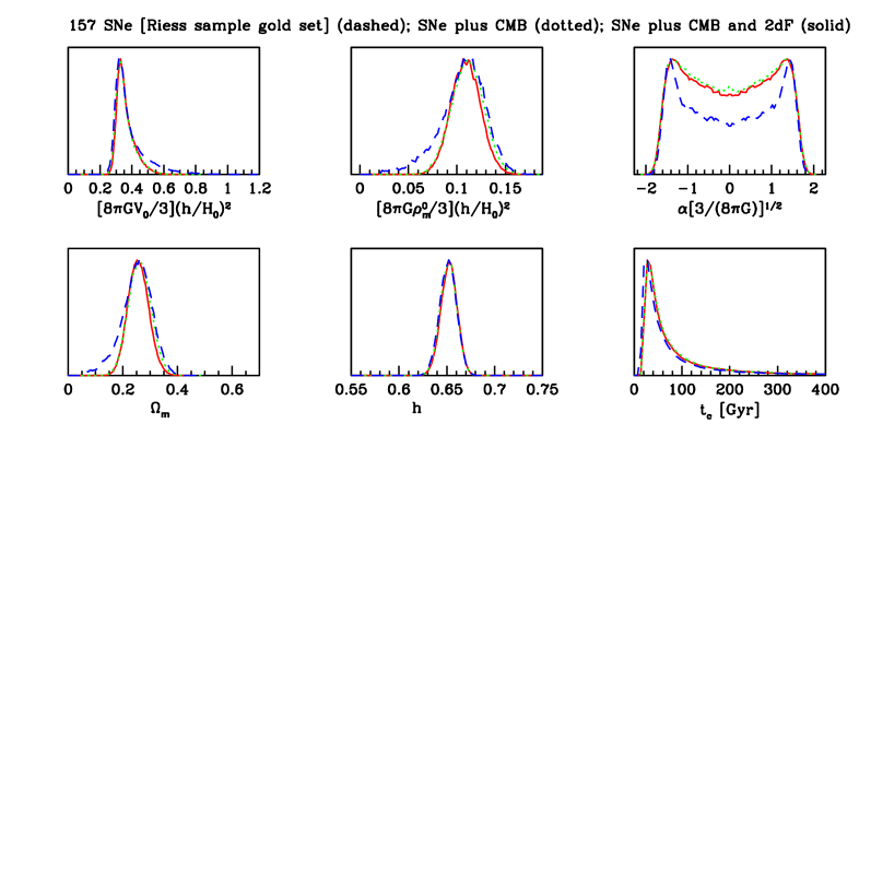
Figure 1: The constraints on the linear model parameters from current SN data only (Riess sample gold set, flux-averaged with $\Delta z=0.05$) (dashed lines), SN together with CMB data (dotted lines), SN together with CMB and LSS data (solid lines). Uniform priors on ($\rho_{m}^{0}$, $V_{0}$, $\alpha$) are assumed. The first row shows the probability distribution functions of the set of independent parameters $V_{0}$, $\rho_{m}^{0}$, and $\alpha$ The second row shows derived parameters $\Omega_{m}$, $h$, and the time to collapse from today $t_{c}$.

Fig.1 shows the constraints on the linear model from current observational data, assuming uniform priors on ($\rho_{m}^{0}$, $V_{0}$, $\alpha$). The first row of figures in Fig.1 shows the probability distribution functions of the set of independent parameters $V_{0}$, $\rho_{m}^{0}$, and $\alpha$. The second row of figures in Fig.1 shows derived parameters $\Omega_{m}$, $h$, and the time to collapse from today $t_{c}$. The dashed lines denote results using SN data only, the dotted lines denote results using SN together with CMB data, the solid lines denote results using SN together with CMB and LSS data.

Table 1 lists the mean and the 68% and 95% confidence ranges of $\Omega_{m}$, $h$, $\alpha$, and $t_{c}$ from Fig.1.

Table 1
The constraints on the linear potential dark energy model from current data
  SN only^a   SN plus CMB^b   SN plus CMB and LSS^c $\Omega_{m}$ $.25\,[.19,.30][.12,.35]\,$ $.26\,[.22,.30][.18,.35]\,$ $.26\,[.22,.30][.19,.33]\,$ $h^{d}$ $.651\,[.642,.660][.634,.668]\,$ $.651\,[.643,.660][.635,.668]\,$ $.652\,[.644,.661][.635,.668]\,$ $\alpha\left(\frac{3}{8\pi G}\right)^{1/2}$ $0.00\,[-1.30,1.30][-1.60,1.60]\,$ $0.00\,[-1.20,1.20][-1.60,1.60]\,$ $0.00\,[-1.20,1.20][-1.60,1.60]\,$ $t_{c}$/[Gyr]^e   56.01 [35.75, —] [19.18, —]   67.48 [42.95, —] [23.61, —]   65.66 [41.92, —] [23.74, —]            [—, 108.18] [—, 2704.01]            [—, 134.34] [—, 4095.18]            [—, 130.52] [—, 3652.01] $\chi^{2}_{min}$/$N_{dof}^{f}$   25.98/23   26.04 /24   26.16/25

^a Riess sample gold set (157 SNe Ia), flux-averaged with ${\Delta}z=.05$.
^b CMB shift parameter $R\equiv\Omega_{m}^{1/2}\Gamma(z_{CMB})=1.716\pm 0.062$.
^c The linear growth rate $f(z_{2dF})=0.51\pm 0.11$.
^d Statistical error only, not including the contribution from the much larger SN Ia absolute magnitude error of $\sigma_{h}^{int}\simeq 0.05$ WangMukherjee .
^e For $t_{c}$, we list median, the 68% and 95% lower bounds and the 68% and 95% upper bounds.
^f The number of degrees of freedom.

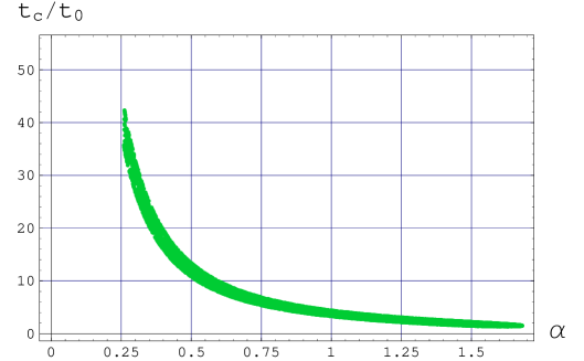
Figure 2: The ratio of the collapse time from today, $t_{c}$, and the age of the universe today, $t_{0}$, as a function of the linear potential parameter $|\alpha|$. Fig.4.

Note that only the median, 68% and 95% confidence lower and upper limits of the collapse time from today $t_{c}$ are given, since $\alpha=0$ is the cosmological constant model with $t_{c}\rightarrow\infty$ (the mean of $t_{c}$ is not well defined for this reason). Computationally, we have to make a cutoff in $t_{c}$ for all models that are longer lived than the computation limit. The dependence of $t_{c}/t_{0}$ on $\alpha$ is shown in Fig.2, where $t_{0}$ is the age of the universe today.

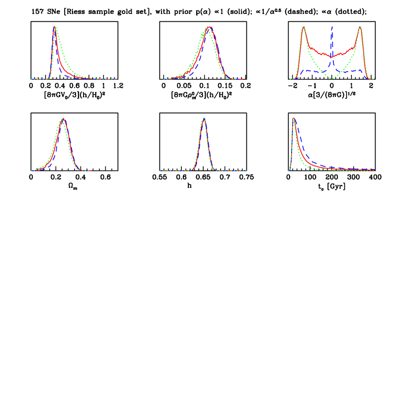
Figure 3: The effect of assuming different priors for $\alpha$, using only SN data (Riess sample gold set, flux-averaged with $\Delta z=0.05$). The parameters are the same as in Fig.1. The solid, dashed, and dotted lines correspond to priors of $p(\alpha)\propto 1$, $\alpha^{-0.5}$, and $\alpha$ respectively.

Fig.3 shows the effect of assuming different priors for $\alpha$, using only SN data (Riess sample gold set, flux-averaged with $\Delta z=0.05$). The parameters are the same as in Fig.1. The solid, dashed, and dotted lines correspond to priors of $p(\alpha)\propto 1$, $\alpha^{-0.5}$, and $\alpha$ respectively. Table 2 shows how assuming different priors for $\alpha$ changes the median, 68% and 95% lower and upper bounds on the collapse time from today $t_{c}$.

Table 2
Effect of assuming different priors for $\alpha$ on the collapse time from today $t_{c}$ (in Gyrs)
$P(\alpha)\propto$ 1 $\alpha^{-0.5}$ $\alpha$ median 56.01 96.92 35.04 68% lower bound 35.75 38.77 27.41 95% lower bound 19.18 19.38 17.91 68% upper bound 108.18 523.35 48.75 95% upper bound 2704.01 714260.81 186.42

IV MCMC versus Fisher Matrix

In this section we compare the joint confidence regions from our MCMC calculations to that of the popular Fisher matrix estimates. The Fisher matrix approach is an easy way to estimate the confidence regions in an $n$-dimensional parameter space $p_{i},$ ($i=1,2,...,n$), and it is especially powerful in the case when the probability distributions are close to the Gaussian distribution. The Fisher matrix is the inverse of the covariance matrix in this $n$-dimensional parameter space, see Fisher :

$$F\equiv C^{-1}.$$

It is easy to calculate the covariance matrix $C$ using the MCMC data and marginalizing over additional parameters. We will consider the distribution and confidence regions for $\alpha$ and $\Omega_{m}.$

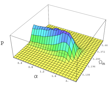
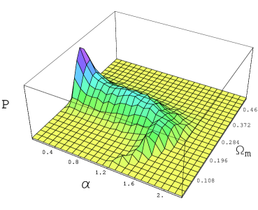
Figure 4: The probability distribution function for the set of parameters $|\alpha|$ and $\Omega_{m}$ with uniform prior on $\alpha$ (left figure) and with the prior proportional to $\alpha^{-0.5}$ (right figure).

In our case, the distribution of the parameter $\alpha$ (slope of the potential) is significantly non-Gaussian (see Fig.1). There are a few facts that we have to take into account. First, the symmetry of the picture is dictated by the fact that the $-\alpha$ and $\alpha$ slopes in Eq.(1) are indistinguishable. It also leads to a paradoxical statement that $\Omega_{m}$ and $\alpha$ parameters become uncorrelated (the corresponding off-diagonal elements of the Fisher matrix are 0). Second, the actual parameter that we are trying to measure, and, hopefully, distinguish from $0$ (cosmological constant case) is actually $|\alpha|.$ This means that in our estimations for joint confidence regions we have to consider absolute value $|\alpha|$ rather than $\alpha.$ In Fig.4 the two-dimensional probability distribution functions for the set of parameters $|\alpha|$ and $\Omega_{m}$ are presented for two different cases - SN plus CMB and LSS data with uniform priors on ($\rho_{m}^{0}$, $V_{0}$, $\alpha$) (right plot) and SN data with $p(\alpha)\propto\alpha^{-0.5}$ (left plot). In both cases the probability distributions are non-Gaussian.

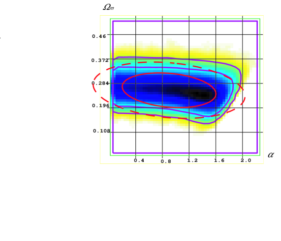
Figure 5: The confidence region for the set of parameters $|\alpha|$ and $\Omega_{m}$. The purple contours are MCMC $68\%$ and $95\%$ regions and red solid (dashed) ellipsoids correspond to $68\%$ ($95\%$) Fisher matrix estimations.

The confidence regions form the Fisher matrix and MCMC method are shown in Fig.5 for SN with CMB and LSS data and uniform priors on ($\rho_{m}^{0}$, $V_{0}$, $\alpha$) (left plot in Fig.4). The MCMC confidence regions are presented by two uneven contours for 1-$\sigma$ (68%) and 2-$\sigma$ (95%) values. Two Fisher ellipses (red solid ellipse corresponds to $68\%$ confidence region and red dashed ellipse corresponds to $95\%$ region) are shown as well. It is clear that due to the non-Gaussian nature of the distribution the Fisher ellipses could be used only for very rough estimations of the confidence regions. In fact, according to Fig.5, $\alpha=0$ (the cosmological constant case) would be excluded at 1-$\sigma$ level for the Fisher matrix approach, that is clearly not the case from the MCMC results. The 2-$\sigma$ regions for both cases give similar results for $\alpha=0$ and $10\%$ discrepancy for the upper bound on $|\alpha|$.

V Predictions from Model-Independent Bounds on the Past Evolution

We now derive complementary bounds on the cosmic doomsday by finding linear potential models that fit completely under the 68% and 95% confidence contours of the model-independent reconstruction of dark energy density $\rho_{X}(z)$ from Ref.WangTegmark .

The idea is to map out the boundaries of the past behavior of $\rho_{X}(z)$ in a model-independent way based on SN Ia and other observations, in this case by the means of splines. Splines have the advantage over polynomials, for instance, that they do not have the tendency to wiggle in between measurement points. While the results will depend somewhat on the type of splines used, i.e. on the number of parameters (the more parameters one uses, the more information is extracted from the data, but the weaker the constraints will become), it is important to realize how this approach differs from earlier, conventional, model-dependent studies. The splines approach is able to model any arbitrary function, not making any assumption about the functional form of $\rho_{X}(z)$ or $w_{X}(z)$, contrary to the practice prevailing in present literature of using two parameter fits.

As a starting point for our study, we take the model-independent boundaries on the past evolution of $\rho_{X}(z)/\rho_{X}(0)$ obtained in WangTegmark . Next, we solve the differential equations for the evolution history of the universe with the linear potential for all possible initial conditions for the scalar field consistent with the $95\%$ and $68\%$ confidence regions of $\Omega_{m}$, and fit their corresponding past $\rho_{X}(z)/\rho_{X}(0)$ history into the above envelope. The model parameters yielding the shortest lifetime, but still not being in violation anywhere with this envelope, determine the minimal lifetime obtainable by this method. These limiting cases, together with the boundaries, are graphically represented in Fig.6.

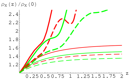
Figure 6: The model-independent constraints on the past of $\rho_{X}(z)/\rho_{X}(0)$ and how they constrain the linear model. The bounds are represented by thick lines, while the corresponding linear model is shown by thin lines with same color and same texture (same dashing). Green denotes the 3-parameter spline bound and its linear model, while red shows the 4-parameter splines. The dashed lines depict the 68% confidence level, while the solid lines stand for 95%. Since the 3-parameter constraint contours always lie inside the 4-parameter spline at a given confidence level, one can argue that the 3-spline investigation is sufficient for this analysis, yielding a minimal future lifetime of $20.6$ Gyr at 95% confidence level.

Our approach is different from WangTegmark in that we recognize that an accurate prediction of the future can only be obtained by a model-specific extrapolation. One can study the past model-independently, yet whatever the conclusion from it is, the future will always depend on the specific underlying physical model. Even in the absence of knowledge of the exact physics—as it is the case presently with dark energy—one is forced to assume a specific physical model to obtain a prediction on the future lifetime of the universe. In our case, the model is the scalar field linear potential.

We use the Hubble time $H_{0}^{-1}$ as the time scale in our calculations. To translate the lifetime into Gyr, we need the value of the Hubble constant $H_{0}$. The Hubble constant, as obtained from the model-independent analysis in WangTegmark , has a mean value of $H_{0}=63.7\rm{km/s/Mpc}$, corresponding to a Hubble time $H_{0}^{-1}=15.36\rm{Gyr}$, for the 3-parameter splines, while $H_{0}=63.5\rm{km/s/Mpc}$ ($H_{0}^{-1}=15.41\rm{Gyr}$) for the 4-parameter spline.

Even the $95\%$ error bars of the distribution for $h$ do not cause an uncertainty of more than $5.7\%$, corresponding to $0.87\mathrm{Gyr}$, thus we will neglect this uncertainty in our lifetime calculation in this section.

In this manner, we obtain for the future lifetime of the universe:

Table 3
The lower bound on future lifetime of the universe
 
Spline Type Confidence Level Future Lifetime 4-parameter 95% lower bound 18.1 Gyr $68\%$ lower bound 22.2 Gyr 3-parameter $95\%$ lower bound 20.6 Gyr $68\%$ lower bound 25.3 Gyr

These results turn out to be a little weaker than our model-specific analysis above. This is not unexpected; it will be very difficult, if not impossible, to close the gap and raise the model-independent analysis to the same accuracy level as the model-dependent one. After all, no assumption about the model in the past is made.

The model-independent analysis also depends on the number of free parameters used. The difference in results between the 3-parameter and the 4-parameter spline is roughly $10\%$. As usual, stronger constraints are achieved by fewer parameters at the cost of less flexibility. Since the 3-parameter spline contour lies completely within the 4-parameter one, one can argue that for the studied sample of supernovae using 3-parameter splines is sufficient.

We conclude that the results obtained by the model-independent study of the past are somewhat less stringent than our results obtained in Sec. III. Indeed, constraining the parameters of a given model directly is the most precise way to proceed. However, it is quite convenient to have a model-independent analysis of the past, and then apply it to any particular model for a quick estimate of the lifetime of the universe. This method provides a useful shortcut, which lets one to obtain approximate results without having to employ the whole machinery of MCMC that we have used to obtain our results in Sec. III.

VI Discussion and Summary

We have studied a representative dark energy model with a linear potential, $V(\phi)=V_{0}(1+\alpha\phi)$, assuming a flat universe. This model has the interesting property of dooming the universe to a Big Crunch for $\alpha\neq 0$. It is the simplest doomsday model, in which the universe collapses rather quickly after it stops expanding.

Since this model has only one free parameter, $\alpha V_{0}$, it is well constrained even by SN Ia data alone (Riess sample), see Fig.1.

We studied this model using current SN Ia (Riess sample), CMB (WMAP, CBI, and ACBAR), and LSS (2dF) data. We have used flux-averaging to minimize the effect of weak lensing Wang00b ; WangMukherjee , and included CMB and galaxy survey data in a consistent manner WangTegmark . We found that in the context of the model with $V(\phi)=V_{0}(1+\alpha\phi)$, observations imply that the cosmic doomsday is more than about 42 billion years from today at 68% confidence, and more than about 24 billion years from today at at the 95% confidence level.

These results represent a stronger bound on the doomsday time than the estimate of $t_{c}\gtrsim 11$ Gyr based on the previously available observational data Kalloshetal . When the data from SNAP and Planck satellites become available, it will be possible to further strengthen our bound up to $t_{c}\gtrsim$ 40 Gyr at 95% confidence Kalloshetal . Note that these timescales have been derived assuming a uniform prior on $\alpha$ (the parameter of the linear model).

When one evaluates the cosmological consequences of a given theory, one should specify not only its Lagrangian and the cosmological initial conditions, but also the theoretical expectations (priors) for the values of the parameters in the model. Since the change of the prior on the parameters is equivalent to changing the underlying physical model, there is nothing surprising in the dependence of the final results on the choice of the prior. For example, if one assumes, on the basis of some physical theory, that the cosmological constant is given by $|\Lambda|=e^{\gamma}$, and all values of $\gamma=\ln|\Lambda|$ are equally probable, one would come to a conclusion that the prior probability for $\Lambda$ is strongly peaked at $\Lambda=0$. This would completely change not only the most probable value of dark energy density obtained from supernova experiments by using MCMC method, but also the famous anthropic bounds on $\Lambda$. However, in the absence of convincing theoretical arguments in favor of the uniform prior for $\ln\Lambda$, one usually assumes uniform or nearly uniform prior for $\Lambda$.

Similarly, the main emphasis of our work was on the study of the linear model with the uniform prior for $\alpha$. To make our results more general and robust, we have also considered other physically motivated priors on $\alpha$ as well, based on Garriga:2003hj . Changing the prior on $\alpha$ can change the bounds on the cosmic doomsday. We found that taking different priors, $p(\alpha)\sim\alpha$ and $p(\alpha)\sim\alpha^{-0.5}$, altered the 95% confidence lower bound on $t_{c}$ obtained for $p(\alpha)=const$ only by about 10%. If one assume the uniform prior for $\ln|\alpha|$, one would conclude that the universe will live for an exponentially long time GV ; Garriga:2003hj . However, if, just as in the case with the cosmological constant, one leaves theoretical speculations aside, one may want to concentrate on the results of our investigation with the uniform prior for $\alpha$.

Interestingly, we were able to obtain not only the lower bound on the doomsday time, but the upper bound as well. For the uniform prior on $\alpha$ the full bound on the doomsday time is $24\ {\rm Gyr}<t_{c}<3652$ Gyr at the 95% confidence level (SN Ia plus CMB and LSS data, see Table 1). In other words, if one believes that the dark energy is described by the simplest linear model, and the parameter $\alpha$ can take any value with equal probability, then our universe most probably will not collapse earlier than in $24$ billion years, but it will most probably live no longer than $3.65\times 10^{3}$ billion years. This doomsday prediction is model-dependent: it is a consequence of our assumption that dark energy is described by the linear model (1), and that all values of the parameter $\alpha$ are equally probable. On the other hand, as we already mentioned, this model is rather generic; it is the simplest representative of a broad class of the dark energy models where the effective cosmological constant can change continuously and the cosmological constant problem can be solved using anthropic considerations Linde ; GV ; Kallosh ; Garriga:2003hj . To improve our constraints on the cosmic doomsday time in this class of models one would need further cosmological observations and a deeper understanding of the theory of dark energy.

- (1) A. G. Riess et al. [Supernova Search Team Collaboration], “Observational Evidence from Supernovae for an Accelerating Universe and a Cosmological Constant,” Astron. J. 116, 1009 (1998) [arXiv:astro-ph/9805201].
- (2) S. Perlmutter et al. [Supernova Cosmology Project Collaboration], “Measurements of Omega and Lambda from 42 High-Redshift Supernovae,” Astrophys. J. 517, 565 (1999) [arXiv:astro-ph/9812133].
- (3) T. Banks, “T C P, Quantum Gravity, The Cosmological Constant And All That..,” Nucl. Phys. B 249, 332 (1985).
- (4) A. D. Linde, “Inflation And Quantum Cosmology,” Print-86-0888 (June 1986), in: “Three hundred years of gravitation”, (Eds.: S. W. Hawking and W. Israel, Cambridge Univ. Press, 1987), 604-630. SPIRES entry
- (5) C. Wetterich, “Cosmology And The Fate Of Dilatation Symmetry,” Nucl. Phys. B 302, 668 (1988); P. J. E. Peebles and B. Ratra, “Cosmology With A Time Variable Cosmological ’Constant’,” Astrophys. J. 325, L17 (1988); J. A. Frieman, C. T. Hill, A. Stebbins and I. Waga, “Cosmology with ultralight pseudo Nambu-Goldstone bosons,” Phys. Rev. Lett. 75, 2077 (1995) [arXiv:astro-ph/9505060]; R. R. Caldwell, R. Dave and P. J. Steinhardt, “Cosmological Imprint of an Energy Component with General Equation-of-State,” Phys. Rev. Lett. 80, 1582 (1998) [arXiv:astro-ph/9708069].
- (6) L. Parker and A. Raval, “Non-perturbative effects of vacuum energy on the recent expansion of the universe,” Phys. Rev. D 60, 063512 (1999) [Erratum-ibid. D 67, 029901 (2003)] [arXiv:gr-qc/9905031]; C. Deffayet, “Cosmology on a brane in Minkowski bulk,” Phys. Lett. B 502, 199 (2001) [arXiv:hep-th/0010186]; K. Freese and M. Lewis, “Cardassian Expansion: a Model in which the Universe is Flat, Matter Dominated, and Accelerating,” Phys. Lett. B 540, 1 (2002) [arXiv:astro-ph/0201229]; S. Mukohyama and L. Randall, “A dynamical approach to the cosmological constant,” Phys. Rev. Lett. 92, 211302 (2004) [arXiv:hep-th/0306108].
- (7) S. Kachru, R. Kallosh, A. Linde and S. P. Trivedi, “De Sitter vacua in string theory,” Phys. Rev. D 68, 046005 (2003) [arXiv:hep-th/0301240]; C. P. Burgess, R. Kallosh and F. Quevedo, “de Sitter string vacua from supersymmetric D-terms,” JHEP 0310, 056 (2003) [arXiv:hep-th/0309187].
- (8) T. Padmanabhan, “Cosmological constant: The weight of the vacuum,” Phys. Rept. 380, 235 (2003) [arXiv:hep-th/0212290]; P. J. E. Peebles and B. Ratra, “The cosmological constant and dark energy,” Rev. Mod. Phys. 75, 559 (2003) [arXiv:astro-ph/0207347].
- (9) A. G. Riess et al. [Supernova Search Team Collaboration], “Type Ia Supernova Discoveries at From the Hubble Space Telescope: Evidence for Past Deceleration and Constraints on Dark Energy Evolution,” Astrophys. J. 607, 665 (2004) [arXiv:astro-ph/0402512].
- (10) Y. Wang and M. Tegmark, “New dark energy constraints from supernovae, microwave background and galaxy clustering,” Phys. Rev. Lett. 92, 241302 (2004) [arXiv:astro-ph/0403292].
- (11) H. K. Jassal, J. S. Bagla and T. Padmanabhan, “WMAP constraints on low redshift evolution of dark energy,” arXiv:astro-ph/0404378.
- (12) D. Huterer and A. Cooray, “Uncorrelated Estimates of Dark Energy Evolution,” arXiv:astro-ph/0404062.
- (13) Y. Wang and K. Freese, “Probing dark energy using its density instead of its equation of state,” arXiv:astro-ph/0402208.
- (14) Y. Wang and P. Mukherjee, “Model-Independent Constraints on Dark Energy Density from Flux-averaging Analysis of Type Ia Supernova Data,” Astrophys. J. 606, 654 (2004) [arXiv:astro-ph/0312192].
- (15) R. A. Daly and S. G. Djorgovski, “Direct Determination of the Kinematics of the Universe and Properties of the Dark Energy as Functions of Redshift,” arXiv:astro-ph/0403664.
- (16) S. Matarrese, C. Baccigalupi and F. Perrotta, “Approaching Lambda without fine-tuning,” arXiv:astro-ph/0403480; U. Alam, V. Sahni and A. A. Starobinsky, “The case for dynamical dark energy revisited,” JCAP 0406, 008 (2004) [arXiv:astro-ph/0403687]; Y. G. Gong, X. M. Chen and C. K. Duan, “A new alternative model to dark energy,” Mod. Phys. Lett. A 19, 1933 (2004) [arXiv:astro-ph/0404202]; B. Feng, X. L. Wang and X. M. Zhang, “Dark Energy Constraints from the Cosmic Age and Supernova,” arXiv:astro-ph/0404224; O. Elgaroy and T. Multamaki, “Cosmic acceleration and extra dimensions: Constraints on modifications of the Friedmann equation,” arXiv:astro-ph/0404402.
- (17) A. D. Linde, “The Inflationary Universe,” Rept. Prog. Phys. 47, 925 (1984).
- (18) J. D. Barrow and F. J. Tipler, “The Anthropic Cosmological Principle,” Oxford University Press, New York 1986.
- (19) S. Weinberg, “Anthropic Bound On The Cosmological Constant,” Phys. Rev. Lett. 59, 2607 (1987); H. Martel, P. R. Shapiro and S. Weinberg, “Likely Values of the Cosmological Constant,” Astrophys. J. 492, 29 (1998) [arXiv:astro-ph/9701099].
- (20) J. Garriga, M. Livio and A. Vilenkin, “The cosmological constant and the time of its dominance,” Phys. Rev. D 61, 023503 (2000) [arXiv:astro-ph/9906210]; J. Garriga and A. Vilenkin, “On likely values of the cosmological constant,” Phys. Rev. D 61, 083502 (2000) [arXiv:astro-ph/9908115]; J. Garriga and A. Vilenkin, “Solutions to the cosmological constant problems,” Phys. Rev. D 64, 023517 (2001) [arXiv:hep-th/0011262].
- (21) J. F. Donoghue, “Random values of the cosmological constant,” JHEP 0008, 022 (2000) [arXiv:hep-ph/0006088]; S. A. Bludman and M. Roos, “Quintessence cosmology and the cosmic coincidence,” Phys. Rev. D 65, 043503 (2002) [arXiv:astro-ph/0109551]; A. Linde, “Inflation, quantum cosmology and the anthropic principle,” arXiv:hep-th/0211048.
- (22) R. Kallosh, A. Linde, S. Prokushkin and M. Shmakova, “Supergravity, dark energy and the fate of the universe,” Phys. Rev. D 66, 123503 (2002) [arXiv:hep-th/0208156]; R. Kallosh and A. Linde, “M-theory, cosmological constant and anthropic principle,” Phys. Rev. D 67, 023510 (2003) [arXiv:hep-th/0208157].
- (23) R. Kallosh and A. Linde, “Dark energy and the fate of the universe,” JCAP 0302, 002 (2003) [arXiv:astro-ph/0301087].
- (24) J. Garriga, A. Linde and A. Vilenkin, “Dark energy equation of state and anthropic selection,” Phys. Rev. D 69, 063521 (2004) [arXiv:hep-th/0310034].
- (25) G. N. Felder, A. Frolov, L. Kofman and A. Linde, “Cosmology with negative potentials,” Phys. Rev. D 66, 023507 (2002) [arXiv:hep-th/0202017].
- (26) R. Bousso and J. Polchinski, “Quantization of four-form fluxes and dynamical neutralization of the cosmological constant,” JHEP 0006, 006 (2000) [arXiv:hep-th/0004134].
- (27) L. Susskind, “The anthropic landscape of string theory,” arXiv:hep-th/0302219.
- (28) M. R. Douglas, “The statistics of string / M theory vacua,” JHEP 0305, 046 (2003) [arXiv:hep-th/0303194].
- (29) R. Kallosh and A. Linde, “Landscape, the scale of SUSY breaking, and inflation,” arXiv:hep-th/0411011.
- (30) R. Kallosh, J. Kratochvil, A. Linde, E. V. Linder and M. Shmakova, “Observational Bounds on Cosmic Doomsday,” JCAP 0310, 015 (2003) [arXiv:astro-ph/0307185].
- (31) U. Alam, V. Sahni and A. A. Starobinsky, “Is dark energy decaying?,” JCAP 0304, 002 (2003) [arXiv:astro-ph/0302302].
- (32) S. Dimopoulos and S. Thomas, “Discretuum versus continuum dark energy,” Phys. Lett. B 573, 13 (2003) [arXiv:hep-th/0307004].
- (33) J. Garriga and A. Vilenkin, “Testable anthropic predictions for dark energy,” Phys. Rev. D 67, 043503 (2003) [arXiv:astro-ph/0210358].
- (34) C. L. Bennett et al., “First Year Wilkinson Microwave Anisotropy Probe (WMAP) Observations: Preliminary Maps and Basic Results,” Astrophys. J. Suppl. 148, 1 (2003) [arXiv:astro-ph/0302207]; D. N. Spergel et al. [WMAP Collaboration], “First Year Wilkinson Microwave Anisotropy Probe (WMAP) Observations: Determination of Cosmological Parameters,” Astrophys. J. Suppl. 148, 175 (2003) [arXiv:astro-ph/0302209].
- (35) M. Tegmark et al. [SDSS Collaboration], “Cosmological parameters from SDSS and WMAP,” Phys. Rev. D 69, 103501 (2004) [arXiv:astro-ph/0310723].
- (36) Y. Wang, “Flux-averaging Analysis of Type Ia Supernova Data,” Astrophys. J. 536, 531 (2000) [arXiv:astro-ph/9907405].
- (37) R. Kantowski, T. Vaughan and D. Branch, “The Effects of Inhomogeneities on Evaluating the Deceleration Parameter q0,” Astrophys. J. 447, 35 (1995) [arXiv:astro-ph/9511108]; J. A. Frieman, Comments Astrophys. 18, 323 (1997); J. Wambsganss, R. Cen, G. Xu, J. P. Ostriker, Astrophys. J. 475, L81; D. E. Holz and R. M. Wald, “A New method for determining cumulative gravitational lensing effects in inhomogeneous universes,” Phys. Rev. D 58, 063501 (1998) [arXiv:astro-ph/9708036]; R. B. Metcalf and J. Silk, “A fundamental test of the nature of dark matter,” Astrophys. J. 519, L1 (1999) [arXiv:astro-ph/9901358]; Y. Wang, “Analytical Modeling of the Weak Lensing of Standard Candles,” Astrophys. J. 525, 651 (1999) [arXiv:astro-ph/9901212]; Y. Wang, D. E. Holz and D. Munshi, “A universal probability distribution function for weak-lensing amplification,” Astrophys. J. 572, L15 (2002) [arXiv:astro-ph/0204169]; Y. Wang, J. Tenbarge and B. Fleshman, “Simple and Accurate Formulae for Distances in Inhomogeneous Universes,” arXiv:astro-ph/0307415.
- (38) R. A. Knop et al., “New Constraints on , , and w from an Independent Set of Eleven High-Redshift Supernovae Observed with HST,” Astrophys. J. 598, 102 (2003) [arXiv:astro-ph/0309368].
- (39) J. R. Bond, G. Efstathiou and M. Tegmark, “Forecasting Cosmic Parameter Errors from Microwave Background Anisotropy Experiments,” Mon. Not. Roy. Astron. Soc. 291, L33 (1997) [arXiv:astro-ph/9702100].
- (40) T. J. Pearson et al., “The Anisotropy of the Microwave Background to l = 3500: Mosaic Observations with the Cosmic Background Imager,” Astrophys. J. 591, 556 (2003) [arXiv:astro-ph/0205388]; C. l. Kuo et al. [ACBAR collaboration], “High Resolution Observations of the CMB Power Spectrum with ACBAR,” Astrophys. J. 600, 32 (2004) [arXiv:astro-ph/0212289].
- (41) E. Hawkins et al., “The 2dF Galaxy Redshift Survey: correlation functions, peculiar velocities and the matter density of the Universe,” Mon. Not. Roy. Astron. Soc. 346, 78 (2003) [arXiv:astro-ph/0212375];
- (42) L. Verde et al., “The 2dF Galaxy Redshift Survey: The bias of galaxies and the density of the Universe,” Mon. Not. Roy. Astron. Soc. 335, 432 (2002) [arXiv:astro-ph/0112161].
- (43) A. Lewis and S. Bridle, “Cosmological parameters from CMB and other data: a Monte-Carlo approach,” Phys. Rev. D 66, 103511 (2002) [arXiv:astro-ph/0205436].
- (44) A. Gelman and D. B. Rubin, “Inference from Iterative Simulation Using Multiple Sequences,” Statistical Science, 7, 457 (1992)
- (45) L. Verde et al., “WMAP: Parameter Estimation Methodology,” Astrophys. J. Suppl., 148, 195 (2003)
- (46) R. A. Fisher, J. Roy. Stat. Soc. 98, 39; M. Tegmark, A. Taylor and A. Heavens, “Karhunen-Loeve eigenvalue problems in cosmology: how should we tackle large data sets?,” Astrophys. J. 480, 22 (1997) [arXiv:astro-ph/9603021].
- (47) B. A. Bassett, P. S. Corasaniti and M. Kunz, “The essence of quintessence and the cost of compression,” arXiv:astro-ph/0407364.
- (48) D. Branch, “Type Ia Supernovae and the Hubble Constant,” Annual Review of Astronomy & Astrophysics, 36, 17 (1998) [arXiv:astro-ph/9801065].
- (49) W. L. Freedman et al., “Final Results from the Hubble Space Telescope Key Project to Measure the Hubble Constant,” Astrophys. J. 553, 47 (2001) [arXiv:astro-ph/0012376].