This document can be cited as: Draine, B.T., and Flatau, P.J. 2004,
“User Guide for the Discrete Dipole Approximation Code DDSCAT 6.1”,
http://arxiv.org/abs/astro-ph/0409262
User Guide for the Discrete Dipole
Approximation Code DDSCAT 6.1

Abstract

DDSCAT 6.1 is a freely available software package which applies the “discrete dipole approximation” (DDA) to calculate scattering and absorption of electromagnetic waves by targets with arbitrary geometries and complex refractive index. The DDA approximates the target by an array of polarizable points. DDSCAT 6.1 allows accurate calculations of electromagnetic scattering from targets with “size parameters” $2\pi a_{\rm eff}/\lambda<15$ provided the refractive index $m$ is not large compared to unity ($|m-1|<2$). DDSCAT 6.1 includes the option of using the FFTW (Fastest Fourier Transform in the West) package. DDSCAT 6.1 also includes support for MPI (Message Passing Interface), permitting parallel calculations on multiprocessor systems.

We also make available a “plain” distribution of DDSCAT 6.1 that does not include support for MPI, FFTW, or netCDF, but is much simpler to install than the full distribution.

The DDSCAT package is written in Fortran and is highly portable. The program supports calculations for a variety of target geometries (e.g., ellipsoids, regular tetrahedra, rectangular solids, finite cylinders, hexagonal prisms, etc.). Target materials may be both inhomogeneous and anisotropic. It is straightforward for the user to “import” arbitrary target geometries into the code, and relatively straightforward to add new target generation capability to the package. DDSCAT automatically calculates total cross sections for absorption and scattering and selected elements of the Mueller scattering intensity matrix for specified orientation of the target relative to the incident wave, and for specified scattering directions.

This User Guide explains how to use DDSCAT 6.1 to carry out electromagnetic scattering calculations. CPU and memory requirements are described.

1 Introduction

DDSCAT 6.1 is a Fortran software package to calculate scattering and absorption of electromagnetic waves by targets with arbitrary geometries using the “discrete dipole approximation” (DDA). In this approximation the target is replaced by an array of point dipoles (or, more precisely, polarizable points); the electromagnetic scattering problem for an incident periodic wave interacting with this array of point dipoles is then solved essentially exactly. The DDA (sometimes referred to as the “coupled dipole approximation”) was apparently first proposed by Purcell & Pennypacker (1973). DDA theory was reviewed and developed further by Draine (1988), Draine & Goodman (1993), and recently reviewed by Draine & Flatau (1994) and Draine (2000).

DDSCAT 6.1 is a Fortran implementation of the DDA developed by the authors.

It is intended to be a versatile tool, suitable for a wide variety of applications ranging from interstellar dust to atmospheric aerosols. As provided, DDSCAT 6.1 should be usable for many applications without modification, but the program is written in a modular form, so that modifications, if required, should be fairly straightforward.

The authors make this code openly available to others, in the hope that it will prove a useful tool. We ask only that:

• If you publish results obtained using DDSCAT, please acknowledge the source of the code.

• If you discover any errors in the code or documentation, please promptly communicate them to the authors.

• You comply with the “copyleft” agreement (more formally, the GNU General Public License) of the Free Software Foundation: you may copy, distribute, and/or modify the software identified as coming under this agreement. If you distribute copies of this software, you must give the recipients all the rights which you have. See the file doc/copyleft distributed with the DDSCAT software.

We also strongly encourage you to send email to the authors identifying yourself as a user of DDSCAT; this will enable the authors to notify you of any bugs, corrections, or improvements in DDSCAT.

The current version, DDSCAT 6.1, uses the DDA formulae from Draine (1988), with dipole polarizabilities determined from the Lattice Dispersion Relation (Draine & Goodman 1993). The code incorporates Fast Fourier Transform (FFT) methods (Goodman, Draine, & Flatau 1991).

We refer you to the list of references at the end of this document for discussions of the theory and accuracy of the DDA [first see the recent reviews by Draine and Flatau (1994) and Draine (2000)]. In §4 we describe the principal changes between DDSCAT 6.1 and the previous releases. The succeeding sections contain instructions for:

• compiling and linking the code;

• running a sample calculation;

• understanding the output from the sample calculation;

• modifying the parameter file to do your desired calculations;

• specifying target orientation;

• changing the DIMENSIONing of the source code to accommodate your desired calculations.

The instructions for compiling, linking, and running will be appropriate for a UNIX system; slight changes will be necessary for non-UNIX sites, but they are quite minor and should present no difficulty.

Finally, the current version of this User Guide can be obtained from
http://arxiv.org/abs/astro-ph/0008151 – you will be offered the options of downloading either Postscript or PDF versions of the User Guide.

2 Applicability of the DDA

The principal advantage of the DDA is that it is completely flexible regarding the geometry of the target, being limited only by the need to use an interdipole separation $d$ small compared to (1) any structural lengths in the target, and (2) the wavelength $\lambda$. Numerical studies (Draine & Goodman 1993; Draine & Flatau 1994; Draine 2000) indicate that the second criterion is adequately satisfied if

$$|m|kd<1~{}~{}~{},$$ (1)

where $m$ is the complex refractive index of the target material, and $k\equiv 2\pi/\lambda$, where $\lambda$ is the wavelength in vacuo. However, if accurate calculations of the scattering phase function (e.g., radar or lidar cross sections) are desired, a more conservative criterion

$$|m|kd<0.5$$ (2)

will ensure that differential scattering cross sections $dC_{\rm sca}/d\Omega$ are accurate to within a few percent of the average differential scattering cross section $C_{\rm sca}/4\pi$ (see Draine 2000).

Let $V$ be the target volume. If the target is represented by an array of $N$ dipoles, located on a cubic lattice with lattice spacing $d$, then

$$V=Nd^{3}~{}~{}~{}.$$ (3)

We characterize the size of the target by the “effective radius”

$$a_{\rm eff}\equiv(3V/4\pi)^{1/3}~{}~{}~{},$$ (4)

the radius of an equal volume sphere. A given scattering problem is then characterized by the dimensionless “size parameter”

$$x\equiv ka_{\rm eff}=\frac{2\pi a_{\rm eff}}{\lambda}~{}~{}~{}.$$ (5)

The size parameter can be related to $N$ and $|m|kd$:

$$x\equiv{2\pi a_{\rm eff}\over\lambda}={62.04\over|m|}\left({N\over 10^{6}}\right)^{1/3}\cdot|m|kd~{}~{}~{}.$$ (6)

Equivalently, the target size can be written

$$a_{\rm eff}=9.873{\lambda\over|m|}\left({N\over 10^{6}}\right)^{1/3}\cdot|m|kd~{}~{}~{}.$$ (7)

Practical considerations of CPU speed and computer memory currently available on scientific workstations typically limit the number of dipoles employed to $N<10^{6}$ (see §16 for limitations on $N$ due to available RAM); for a given $N$, the limitations on $|m|kd$ translate into limitations on the ratio of target size to wavelength.

For calculations of total cross sections $C_{\rm abs}$ and $C_{\rm sca}$, we require $|m|kd<1$:

$$a_{\rm eff}<9.88{\lambda\over|m|}\left({N\over 10^{6}}\right)^{1/3}{\rm~{}~{}or~{}~{}}x<{62.04\over|m|}\left({N\over 10^{6}}\right)^{1/3}~{}~{}~{}.$$ (8)

For scattering phase function calculations, we require $|m|kd<0.5$:

$$a_{\rm eff}<4.94{\lambda\over|m|}\left({N\over 10^{6}}\right)^{1/3}{\rm~{}~{}~{}~{}or~{}~{}~{}~{}}x<{31.02\over|m|}\left({N\over 10^{6}}\right)^{1/3}~{}~{}~{}.$$ (9)

It is therefore clear that the DDA is not suitable for very large values of the size parameter $x$, or very large values of the refractive index $m$. The primary utility of the DDA is for scattering by dielectric targets with sizes comparable to the wavelength. As discussed by Draine & Goodman (1993), Draine & Flatau (1994), and Draine (2000), total cross sections calculated with the DDA are accurate to a few percent provided $N>10^{4}$ dipoles are used, criterion (1) is satisfied, and the refractive index is not too large.

For fixed $|m|kd$, the accuracy of the approximation degrades with increasing $|m-1|$, for reasons having to do with the surface polarization of the target as discussed by Collinge & Draine (2004). With the present code, good accuracy can be achieved for $|m-1|<2$.

Examples illustrating the accuracy of the DDA are shown in Figs. 1–2 which show overall scattering and absorption efficiencies as a function of wavelength for different discrete dipole approximations to a sphere, with $N$ ranging from 304 to 59728. The DDA calculations assumed radiation incident along the (1,1,1) direction in the “target frame”. Figs. 3–4 show the scattering properties calculated with the DDA for $x=ka=7$. Additional examples can be found in Draine & Flatau (1994) and Draine (2000).

Figure 1: Scattering and absorption for a sphere with $m=1.33+0.01i$. The upper panel shows the exact values of $Q_{\rm sca}$ and $Q_{\rm abs}$, obtained with Mie theory, as functions of $x=ka$. The middle and lower panels show fractional errors in $Q_{\rm sca}$ and $Q_{\rm abs}$, obtained using DDSCAT with polarizabilities obtained from the Lattice Dispersion Relation, and labelled by the number $N$ of dipoles in each pseudosphere. After Fig. 1 of Draine & Flatau (1994).

Figure 2: Same as Fig. 1, but for $m=2+i$. After Fig. 2 of Draine & Flatau (1994).

Figure 3: Differential scattering cross section for $m=1.33+0.01i$ pseudosphere and $ka=7$. Lower panel shows fractional error compared to exact Mie theory result. The $N=17904$ pseudosphere has $|m|kd=0.57$, and an rms fractional error in $d\sigma/d\Omega$ of 2.4%. After Fig. 5 of Draine & Flatau (1994).

Figure 4: Same as Fig. 3 but for $m=2+i$. The $N=59728$ pseudosphere has $|m|kd=0.65$, and an rms fractional error in $d\sigma/d\Omega$ of 6.7%. After Fig. 8 of Draine & Flatau (1994).

3 DDSCAT 6.1

3.1 What Does It Calculate?

DDSCAT 6.1, like previous versions of DDSCAT, solves the problem of scattering and absorption by an array of polarizable point dipoles interacting with a monochromatic plane wave incident from infinity. DDSCAT 6.1 has the capability of automatically generating dipole array representations for a variety of target geometries (see §19) and can also accept dipole array representations of targets supplied by the user (although the dipoles must be located on a cubic lattice). The incident plane wave can have arbitrary elliptical polarization (see §21), and the target can be arbitrarily oriented relative to the incident radiation (see §17). The following quantities are calculated by DDSCAT 6.1 :

• Absorption efficiency factor $Q_{\rm abs}\equiv C_{\rm abs}/\pi a_{\rm eff}^{2}$, where $C_{\rm abs}$ is the absorption cross section;

• Scattering efficiency factor $Q_{\rm sca}\equiv C_{\rm sca}/\pi a_{\rm eff}^{2}$, where $C_{\rm sca}$ is the scattering cross section;

• Extinction efficiency factor $Q_{\rm ext}\equiv Q_{\rm sca}+Q_{\rm abs}$;

• Phase lag efficiency factor $Q_{\rm pha}$, defined so that the phase-lag (in radians) of a plane wave after propagating a distance $L$ is just $n_{t}Q_{\rm pha}\pi a_{\rm eff}^{2}L$, where $n_{t}$ is the number density of targets.

• The 4$\times$4 Mueller scattering intensity matrix $S_{ij}$ describing the complete scattering properties of the target for scattering directions specified by the user.

• Radiation force efficiency vector ${\bf Q}_{\rm rad}$ (see §15).

• Radiation torque efficiency vector ${\bf Q}_{\Gamma}$ (see §15).

3.2 Application to Targets in Dielectric Media

Let $\omega$ be the angular frequency of the incident radiation. For many applications, the target is essentially in vacuo, in which case the dielectric function $\epsilon$ which the user should supply to DDSCAT is the actual complex dielectric function $\epsilon_{\rm target}(\omega)$, or complex refractive index $m_{\rm target}(\omega)=\sqrt{\epsilon_{\rm target}}$ of the target material.

However, for many applications of interest (e.g., marine optics, or biological optics) the “target” body is embedded in a (nonabsorbing) dielectric medium, with (real) dielectric function $\epsilon_{\rm medium}(\omega)$, or (real) refractive index $m_{\rm medium}(\omega)=\sqrt{\epsilon_{\rm medium}}$. DDSCAT is fully applicable to these scattering problems, except that:

• The “dielectric function” or “refractive index” supplied to DDSCAT should be the relative dielectric function

  $$\epsilon(\omega)=\frac{\epsilon_{\rm target}(\omega)}{\epsilon_{\rm medium}(\omega)}$$ (10)

  or relative refractive index:

  $$m(\omega)=\frac{m_{\rm target}(\omega)}{m_{\rm medium}(\omega)}.$$ (11)

• The wavelength $\lambda$ specified in ddscat.par should be the wavelength in the medium:

  $$\lambda=\frac{\lambda_{vac}}{m_{\rm medium}},$$ (12)

  where $\lambda_{vac}=2\pi c/\omega$ is the wavelength in vacuo.

The absorption, scattering, extinction, and phase lag efficiency factors $Q_{\rm abs}$, $Q_{\rm sca}$, and $Q_{\rm ext}$ calculated by DDSCAT will then be equal to the physical cross sections for absorption, scattering, and extinction divided by $\pi a_{\rm eff}^{2}$. For example, the attenuation coefficient for radiation propagating through a medium with a number density $n_{t}$ of scatterers will be just $\alpha=n_{t}Q_{\rm ext}\pi a_{\rm eff}^{2}$. Similarly, the phase lag (in radians) after propagating a distance $L$ will be $n_{t}Q_{\rm pha}\pi a_{\rm eff}^{2}$.

The elements $S_{ij}$ of the 4$\times$4 Mueller scattering matrix ${\bf S}$ calculated by DDSCAT will be correct for scattering in the medium:

$${\bf I}_{\rm sca}=\left(\frac{\lambda}{2\pi r}\right)^{2}{\bf S}\cdot{\bf I}_{in},$$ (13)

where ${\bf I}_{in}$ and ${\bf I}_{\rm sca}$ are the Stokes vectors for the incident and scattered light (in the medium), $r$ is the distance from the target, and $\lambda$ is the wavelength in the medium (eq. 12). See §23 for a detailed discussion of the Mueller scattering matrix.

The time-averaged radiative force and torque (see §15) on a target in a dielectric medium are

$${\bf F}_{\rm rad}={\bf Q}_{pr}\pi a_{\rm eff}^{2}u_{\rm rad}~{}~{}~{},$$ (14)

$${\bf\Gamma}_{\rm rad}={\bf Q}_{\Gamma}\pi a_{\rm eff}^{2}u_{\rm rad}\frac{\lambda}{2\pi}~{}~{}~{},$$ (15)

where the time-averaged energy density is

$$u_{\rm rad}=\epsilon_{\rm medium}\frac{E_{0}^{2}}{8\pi}~{}~{}~{},$$ (16)

where $E_{0}\cos(\omega t+\phi)$ is the electric field of the incident plane wave in the medium.

4 What’s New?

DDSCAT 6.1 differs from DDSCAT 5a in the following ways:

1. Via the parameter file ddscat.par, the user can now select up to 9 elements of the Muller scattering matrix $S_{ij}$ to be printed out.

2. The maximum number of iterations allowed has been increased from 300 to 10000, since DDSCAT is now increasingly employed for computations that converge relatively slowly: large numbers of dipoles, large values of the scattering parameter, or large values of the refractive index. The number of iterations used for a solution is recorded in the wwaarbbkccc.sca output files.

3. In the form distributed, DDSCAT writes only buffered output. When run on a single cpu (with MPI disabled), DDSCAT writes “running output” to a file ddscat.log_000. When MPI is enabled, cpu nnn writes to a file ddscat.log_nnn, where n=000,001,002, etc.

4. A new target option is available: LYRSLB (a rectangular slab with up to 4 different material layers).

5. User must now specify (in ddscat.par) which IWAV, IRAD, IWAV to start with. The “default” choice will be 0 0 0, but when computations have been interupted by, e.g., power outage, there will be occasions when it is convenient to be able to resume with the first incomplete calculation.

6. A new FFT option is supported: FFTW21. This invokes the FFTW (“Fastest Fourier Transform in the West”) package of Frigo and Johnson. The calls are compatible with versions 2.1.x of FFTW. Instructions on compiling and linking to include FFTW are given below (§6.2.5).

7. FFT options BRENNR and TMPRTN have been eliminated as they seem to offer no advantages relative to GPFAFT or FFTW21.

8. MPI is now supported. Users can now carry out parallel calculations using DDSCAT 6.1 on multiprocessor systems in conformance with the MPI (Message Passing Interface) standards (§24). This of course requires that MPI be already installed on the system.

9. New with DDSCAT 6.1: calculation of $\langle\cos^{2}\theta\rangle$ for the scattered radiation field, in addition to the first moment $\langle\cos\theta\rangle$. The format of the output files ww$aa$r$bb$k$ccc$.sca has been altered.

10. New with DDSCAT 6.1: The output files written when the NETCDF option is specified have been modified to include more relevant data and to be more easily read.

11. New with DDSCAT 6.1: The procedure used for averaging over scattering angles has been improved, both to improve efficiency and to make it easier for the user to manage the balance between accuracy and computational burden. Via the parameter file ddscat.par, the user now specifies a parameter ETASCA (see §22 for discussion of the relationship between ETASCA and accuracy). Important note: The parameters ICTHM and IPHIM have been eliminated! (See §8 for discussion of the parameter file ddscat.par, or Appendix A for an annotated example of the ddscat.par file). ddscat.par files used with previous releases of DDSCAT will not work until edited to remove ICTHM and IPHIM and add specification of ETASCA!

12. New with DDSCAT 6.1: In addition to the full distribution of DDSCAT 6.1, we also make available a “plain” distribution which does not include support for MPI, FFTW, or netCDF, but is much simpler for a user to compile and install. This “plain” distribution is recommended for first-time users.

13. New with DDSCAT 6.1: A new target option ANIREC is available for homogenous rectangular targets composed of anisotropic material (see §19).

14. New with DDSCAT 6.1: A new target option CYLCAP is available: the target is a cylinder with hemispherical end-caps.

15. 2006.11.28 bug fix: Corrected error in evaluation of $P=$ degree of linear polarization of scattered light. Mueller matrix elements $S_{ij}$ were calculated and reported correctly, but $P$ was not correctly evaluated.

5 Obtaining and Installing the Source Code

5.1 For first-time users: the “plain” distribution

The “plain” distribution lacks support for MPI, FFTW, netCDF, and reporting of cpu time used in different phases of the calculation, but has complete capabilities for target generation and calculating scattering using a single CPU. The “plain” distribution is recommended for first-time users.

5.2 The “full” distribution

If you require support for  MPI,  FFTW,  or  netCDF,  you should download the “full” distribution of DDSCAT 6.1.

5.3 Downloading the Source Code

There are 3 ways to obtain the source code:

• Point your browser to the DDSCAT 6.1 home page:
  http://www.astro.princeton.edu/$\sim$draine/DDSCAT.html
  where you will find links for ddscat6.1_plain.tgz and ddscat6.1_full.tgz, gzipped tarfiles containg the complete source code for the “plain” and “full” distributions, respectively. Right-click on the appropriate link.

• Point your browser to
  ftp://ftp.astro.princeton.edu/draine/scat/ddscat/ver6.1
  right-click on ddscat6.1_plain.tgz  or  ddscat6.1_full.tgz .

• Use anonymous ftp  to  ftp.astro.princeton.edu.
  In response to  “Name:”  enter  anonymous.
  In response to  “Password:”  enter your full email address.
  cd draine/scat/ddscat/ver6.1
  binary   (to enable transfer of binary data
  get ddscat6.1_plain.tgz   (To get the “plain” distribution)
        or
  get ddscat6.1_full.tgz   (To get the “full” distribution).

After downloading either ddscat6.1_plain.tgz or ddscat6.1_full.tgz into the directory where you would like DDSCAT 6.1 to reside (you should have at least 10 Mbytes of disk space available), the source code can be installed as follows:

5.4 Installing the source code on a Linux/Unix system

If you are on a Linux system, you should be able to type
      tar xvzf ddscat6.1_plain.tgz
            or
      tar xvfz ddscat6.1_full.tgz
which will“extract” the files from the gzipped tarfile. If your version of “tar” doesn’t support the “z” option (e.g., you are running Solaris) then try
      zcat ddscat6.1_plain.tgz | tar xvf -
            or
      zcat ddscat6.1_full.tgz | tar xvf -
If neither of the above work on your system, try the two-stage procedure
      gunzip ddscat6.1_plain.tgz
      tar xvf ddscat6.1_plain.tar
            or
      gunzip ddscat6.1_full.tgz
      tar xvf ddscat6.1_full.tar
A disadvantage of this two-stage procedure is that it uses more disk space, since after the second step you will have the uncompressed tarfile ddscat6.1_full.tar – about 3.8 Mbytes – in addition to all the files you have extracted from the tarfile – another 4.6 Mbytes.

Any of the above approaches should create subdirectories src, doc, misc, and IDL. The source code will be in subdirectory src, and documentation in subdirectory doc.

5.5 Installing the source code on a MS Windows system

If you are running Windows on a PC, you will need the “winzip” program. winzip should be able to “unzip” the gzipped tarfile ddscat6.1_plain.tgz or ddscat6.1_full.tgz and “extract” the various files from it automatically.

6 Compiling and Linking

6.1 The “plain” distribution

In the discussion below, it is assumed that the source code for the “plain” distribution of DDSCAT 6.1 has been installed in a directory DDA/src. To compile the code on a Linux system with the g77 compiler, position yourself in the directory DDA/src, and type
      make ddscat
If you are on another type of system, or wish to use a different compiler (or compiler options) you will need to edit the file Makefile to change the choice of compiler (variable FC) compilation options (variables FFLAGS and FFLAGSslamc1, and loader options (variable LDFLAGS).

6.1.1 Compiling the “plain” version on non-Unix systems

DDSCAT 6.1is written in standard Fortran-77 plus the DO ... ENDDO extension which appears to be supported by all current Fortran-77 compatible compilers. It is possible to run DDSCAT on non-Unix systems. If the Unix “make” utility is not available, here in brief is what needs to be accomplished:

All of the necessary Fortran code to compile and link DDSCAT 6.1was included in and should have been extracted from the gzipped tarfile ddscat6.1_plain.tgz. A subset of the files needs to be compiled and linked to produce the ddscat executable.

The main program is in DDSCAT.f ; it calls a number of subroutines.

A number of different versions of SUBROUTINE TIMEIT are included in ddscat6.1_plain.tgz. The easiest course is to use the version in timeit_null.f, which begins

      SUBROUTINE TIMEIT(CMSGTM,DTIME)
C
C     timeit_null
C
C This version of timeit is a dummy which does not provide any
C timing information.

This version does not use any system calls, and therefore the code should compile and link without problems; however, when you run the code, it will not report any timing information reporting how much time was spent on different parts of the calculation.

If you wish to obtain timing information, you will need to find out what system calls are supported by your operating system. You can look at the other versions of SUBROUTINE TIMEIT provided in ddscat6.1_plain.tgz to see how this has been done under VMS and various versions of Unix.

Once you have selected the appropriate version of TIMEIT , you can simply compile and link just as you would with any other Fortran code with a number of modules. You should end up with an executable with a (system-dependent) name like DDSCAT.EXE.

6.1.2 Optimization

The performance of DDSCAT 6.1 will benefit from optimization during compilation and the user should enable the appropriate compiler flags.

There is one exception: the LAPACK routine SLAMC1, which is called to determine the number of bits of precision provided by the computer architectures, should NOT be optimized, because under some optimizers the resulting code will end up in an endless loop. Therefore the Makefile has a separate compilation flag FFLAGSslamc1 which should not specify optimization (e.g., just  g77 -c, or  pgf77 -c).

6.2 The complete distribution

In the discussion below, it will be assumed that the complete source code for DDSCAT 6.1 from ddscat6.1_full.tgz has been installed in a directory DDA/src. To compile the code on a Unix system, position yourself in the directory DDA/src. The as-supplied Makefile has compiler options set as appropriate for

• use of the g77 compiler under the Linux operating system.

• use of a Linux-compatible and Solaris-compatible timing routine.

• FFTW option not enabled

• MPI not enabled

• netCDF not enabled

If you type
      make ddscat
you should be able to compile and link to create an executable ddscat located in this directory. If this does not work with the as-supplied Makefile, the problem is likely due to unavailability of the g77 fortran compiler, or the need to select a different version of the TIMEIT routine (see below). If you have a different Fortran compiler, you will probably need to edit Makefile to provide the desired compiler options. If you are using an operating system other than Linux, you may need to change the Makefile choice of timeit. Makefile contains samples of compiler options for selected operating systems, including Linux, HP AUX, IBM AIX, and SGI IRIX operating systems. If one of these corresponds to your system, try “uncommenting” (i.e., removing the # at the beginning of a line) the appropriate lines in the Makefile.

So far as we know, there are only two operating-system-dependent aspects of DDSCAT 6.1: (1) the device number to use for “standard output”, and (2) the TIMEIT routine. There are, in addition, three installation-dependent aspects to the code:

• the procedure for linking to the FFTW library (see §6.2.5)

• the procedure for linking to the netCDF library (see §10.3 for discussion of the possibility of writing binary files using the machine-independent netCDF standard).

• the procedure for linking to the MPI library (see §24.2).

6.2.1 Device Numbers IDVOUT and IDVERR

The variables IDVOUT and IDVERR specify device numbers for “running output” and “error messages”, respectively. Normally these would both be set to the device number for “standard output” (e.g., writing to the screen if running interactively). Variables IDVERR are set by DATA statements in the “main” program DDSCAT.f and in the output routine WRIMSG (file wrimsg.f). The executable statement IDVOUT=0 initializes IDVOUT to 0. In the as-distributed version of DDSCAT.f, the statement

OPEN(UNIT=IDVOUT,FILE=CFLLOG)

causes the output to UNIT=IDVOUT to be buffered and written to the file ddscat.log_nnn, where nnn=000 for the first cpu, 001 for the second cpu, etc. If it is desirable to have this output unbuffered for debugging purposes, (so that the output will contain up-to-the-moment information) simply comment out this OPEN statement.

6.2.2 Subroutine TIMEIT

The only other operating system-dependent part of DDSCAT 6.1 is the single subroutine TIMEIT. Several versions of TIMEIT are provided:

• timeit_sun.f uses the SunOS system call etime

• timeit_convex.f uses the Convex OS system call etime

• timeit_cray.f uses the system call second

• timeit_hp.f uses the HP-AUX system calls sysconf and times

• timeit_ibm6000.f uses the AIX system call mclock

• timeit_osf.f uses the DEC OSF system call etime

• timeit_sgi.f uses the IRIX system call etime

• timeit_vms.f uses the VMS system calls LIB$INIT_TIMER and LIB$SHOW_TIMER

• timeit_titan.f uses the system call cputim

• timeit_null.f is a dummy routine which provides no timing information, but can be used under any operating system.

You must compile and link one of the timeit_xxx.f routines, possibly after modifying it to work on your system; timeit_null.f is the easiest choice, but it will return no timing information.

6.2.3 Optimization

The performance of DDSCAT 6.1 will benefit from optimization during compilation and the user should enable the appropriate compiler flags (e.g.,  g77 -c -O, or  pgf77 -c -fast).

There is one exception: the LAPACK routine SLAMC1, which is called to determine the number of bits of precision provided by the computer architectures, should NOT be optimized, because under some optimizers the resulting code will end up in an endless loop. Therefore the Makefile has a separate compilation flag FFLAGSslamc1 which should not specify optimization (e.g., just  g77 -c, or  pgf77 -c).

6.2.4 Leaving FFTW Capability Disabled

FFTW – “Fastest Fourier Transform in the West” – is a publicly available FFT implementation that performs very well (see §13). DDSCAT 6.1 supports use of FFTW, but it is recommended that first-time users of DDSCAT first get the code up and running without FFTW support, using the built-in GPFA FFT routine written by Clive Temperton, which performs almost as well as FFTW. This is also the option you will have to follow if FFTW is not installed on your system (though you can install it yourself, if necessary – see §6.2.5 below).

The Makefile supplied with the DDSCAT 6.1 distribution is initially set up to leave support for FFTW disabled by using a “dummy” subroutine cxfftw_fake.f. When you type make ddscat you will create a version of ddscat which will not recognize option FFTW21 – you must specify option GFPAFT in ddscat.par when running the code.

6.2.5 Enabling FFTW Capability

The FFTW (“Fastest Fourier Transform in the West”) package of Matteo Frigo and Steven G. Johnson appears to be one of the fastest public-domain FFT packages available (see §13 for a performance comparison), and DDSCAT 6.1 allows this package to be used. In order to support the FFTW21 option, however, it is necessary to first install the FFTW package on your system (FFTW 2.1.x – we have not yet implemented support for FFTW 3.0, which has a different interface).

FFTW offers two advantages:

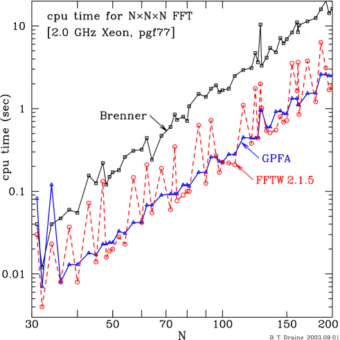
Figure 6: Comparison of cpu time required by 3 different FFT implementations. It is seen that the GPFA and FFTW implementations have comparable speeds, much faster than Brenner’s FFT implementation.

• It appears, for some cases, to be somewhat faster than the GPFA FFT algorithm which is already included in the DDSCAT package (see §13 and Fig. 6).

• It does not restrict the dimensions of the “computational volume” to be factorizable as $2^{i}3^{j}5^{k}$, and therefore for some targets will use a smaller computational volume (and therefore require less memory).

If the FFTW package is not yet installed on your system, then

1. Download the FFTW 2.1.x package from http://www.fftw.org (as of this writing the latest version 2.1.x is fftw-2.1.5.tar.gz) into some convenient directory.

2. tar xvfz fftw-2.1.5.tar.gz

3. cd fftw-2.1.5

4. ./configure --enable-float --enable-type-prefix --prefix=PATH
   where PATH is the path to the directory in which you would like the fftw library installed (you must have write permission, of course). If you choose to omit
               --prefix=PATH
   then fftw will be installed in the default directory /usr/local/, but unless you are root you may not have write permission to this directory.

5. make

6. make install

This should install the file libsfftw.a in the directory /usr/local/lib (or PATH/lib if you used option --prefix=PATH when running configure).

Once FFTW is installed, you will need to edit Makefile (go to section 4, “FFTW support”:

• change the lines

  CXFFTW          = cxfftw_fake
  LIBFFTW         =
  

  to

  #CXFFTW         = cxfftw_fake
  #LIBFFTW        =
  

• Go down a few lines in the Makefile, and change the lines

  #CXFFTW         = cxfftw
  #LIBFFTW        = -L/usr/local/lib -lsfftw
  

  to

  CXFFTW          = cxfftw
  LIBFFTW         = -L/usr/local/lib -lsfftw
  

  LIBFFTW gives the path to libsfftw.a, which is installation-dependent. Consult your local systems administrator.

Once the above is done, typing make ddscat should create an executable ddscat which will recognize option FFTW21 in the file ddscat.par. Note that you will be linking fortran to C, and different compilers may behave idiosyncratically. The Makefile has examples which work for g77 and pgf77. If you have trouble, consult with someone familiar with linking fortran and C modules on your system.

6.2.6 Leaving netCDF Capability Disabled

netCDF is a standard for data transport used at many sites (see §10.3 for more information on netCDF). The Makefile supplied with the distribution of DDSCAT 6.1 is set up to link to a “dummy” subroutine writenet_fake.f instead of subroutine writenet.f, in order to minimize problems during initial compilation and linking. The “dummy” routine has no functionality, other than bailing out with a fatal error message if the user makes the mistake of trying to specify one of the netCDF options (ALLCDF or ORICDF). First-time users of DDSCAT 6.1 should not try to use the netCDF option – simply skip this section, and specify option NOTCDF in ddscat.par. After successfully using DDSCAT 6.1  you can return to §6.2.7 to try to enable the netCDF capability.

6.2.7 Enabling netCDF Capability

Subroutine WRITENET (file writenet.f) provides the capability to output binary data in the netCDF standard format (see §10.3). In order to use this routine (instead of writenet_fake.f), it is necessary to take the following steps:

1. Have netCDF already installed on your system (check with your system administrator).

2. Find out where netcdf.inc is located and edit the include statement in writenet.f to specify the correct path to netcdf.inc.

3. Find out where the libnetcdf.a library is located on your system.

4. Go to section 6 of the Makefile (“netCDF library support”) and

   • edit the lines

     WRITENET      = writenet_fake
     LIBNETCDF     =
     LINKNETCDF    =
     

     to

     #WRITENET      = writenet_fake
     #LIBNETCDF     =
     #LINKNETCDF    =
     

   • Go down a few lines in the Makefile and change

     #WRITENET      = writenet
     #LIBNETCDF     = -L/usr/local/lib
     #LINKNETCDF    = -lnetcdf -lnsl
     

     to

     WRITENET      = writenet
     LIBNETCDF     = -L/usr/local/lib
     LINKNETCDF    = -lnetcdf -lnsl
     

     The second and third lines above work on some systems, but will be installation-dependent; if you get an error message during the link step, consult your systems administrator or someone who has used netCDF on your system.

6.2.8 Compiling and Linking…

After suitably editing the Makefile (while still positioned in DDA/src) simply type make ddscat which should create an executable file DDA/src/ddscat . If the default (as-provided) Makefile is used, the g77 fortran compiler will be used to create an executable which:

• will not have MPI support;

• will not have FFTW support;

• will not have netCDF capability;

• will contain timing instructions compatible with Linux, Solaris, as well as several other flavors of Unix.

To add FFTW capability, see §6.2.5. To add netCDF capability, see §6.2.7. To add MPI support, see §24. To replace the Linux-compatible and Sun-compatible timing routine with another, see §6.2.2.

6.2.9 Installation of the “full” version on non-Unix systems

DDSCAT 6.1is written in standard Fortran-77 plus the DO ... ENDDO extension which appears to be supported by all current Fortran-77 compatible compilers. It is possible to run DDSCAT on non-Unix systems. If the Unix “make” utility is not available, here in brief is what needs to be accomplished:

All of the necessary Fortran code to compile and link DDSCAT 6.1was included in and should have been extracted from the gzipped tarfile ddscat6.1_full.tgz. A subset of the files needs to be compiled and linked to produce the ddscat executable.

The main program is in DDSCAT.f ; it calls a number of subroutines.

Some of the subroutines exist in more than one version.

• Select the version of SUBROUTINE CXFFTW in file cxfftw_fake.f instead of the version in cxfftw.f.  The resulting code will not support FFTW.
  If you later wish to add FFTW capability, you will first need to install the FFTW library on your system (see §6.2.5). After you have done so, you can switch to using the version of SUBROUTINE CXFFTW in cxffwt.f.

• Select the version of SUBROUTINE WRITENET in writenet_fake.f instead of the version in writenet.f.  The resulting code will not provide netCDF capability.
  If netCDF capability is required, you will need to install netCDF libraries on your system – see §6.2.7). After doing so, you can switch to using writenet.f instead of writenet_fake.f.

• Use the code in the file mpi_fake.f instead of that in the file mpi_fake.f. The resulting code will not support MPI.
  If MPI support is required, you will need to install MPI on your system – see §24. After doing so, you can switch to using mpi.f .

• There are a number of different versions of SUBROUTINE TIMEIT included in ddscat6.1_full.tgz. Use the version in timeit_null.f, which begins
  

        SUBROUTINE TIMEIT(CMSGTM,DTIME)
  C
  C     timeit_null
  C
  C This version of timeit is a dummy which does not provide any
  C timing information.
  

  This version does not use any system calls, and therefore the code should compile and link without problems; however, when you run the code, it will not report any timing information reporting how much time was spent on different parts of the calculation.
  If you wish to obtain timing information, you will need to find out what system calls are supported by your operating system. You can look at the other versions of SUBROUTINE TIMEIT provided in ddscat6.1_full.tgz to see how this has been done under VMS and various version of Unix.

Once you have selected the appropriate versions of CXFFTW, WRITENET, TIMEIT, and either mpi_fake.f or mpi.f , you can simply compile and link just as you would with any other Fortran code with a number of modules. You should end up with an executable with a (system-dependent) name like DDSCAT.EXE.

In addition to program DDSCAT, we provide one other Fortran 77 program which may be useful. Program CALLTARGET (in CALLTARGET.f) can be used to call the target generation routines. This is especially helpful when experimenting with new target geometries.

7 Moving the Executable

Now reposition yourself into the directory DDA (e.g., type cd ..), and copy the executable from src/ddscat to the DDA directory by typing

cp src/ddscat ddscat

This should copy the file DDA/src/ddscat to DDA/ddscat (you could, of course, simply create a symbolic link instead). Similarly, copy the sample parameter file ddscat.par and the file diel.tab to the DDA directory by typing

cp doc/ddscat.par ddscat.par cp doc/diel.tab diel.tab

8 The Parameter File ddscat.par

The directory DDA should now contain a sample file ddscat.par which provides parameters to the program ddscat. As provided (see AppendixA), the file ddscat.par is set up to calculate scattering by a 32$\times$24$\times$16 rectangular array of 12288 dipoles, with an effective radius $a_{\rm eff}=2{\mu{\rm m}}$, at a wavelength of $6.2832{\mu{\rm m}}$ (for a “size parameter” $2\pi a_{\rm eff}/\lambda=2$).

The dielectric function of the target material is provided in the file diel.tab, which is a sample file in which the refractive index is set to $m=1.33+0.01i$ at all wavelengths; the name of this file is provided to ddscat by the parameter file ddscat.par.

The sample parameter file as supplied calls for the GPFA FFT routine (GPFAFT) of Temperton (1992) to be employed and the PBCGST iterative method to be used for solving the system of linear equations. (See section §13 and §14 for discussion of choice of FFT algorithm and choice of equation-solving algorithm.)

The sample parameter file specifies (via option LATTDR) that the “Lattice Dispersion Relation” (Draine & Goodman 1993) be employed to determine the dipole polarizabilities. See §11 for discussion of other options.

The sample parameter files specifies options NOTBIN and NOTCDF so that no binary data files and no NetCDF files will be created by ddscat. The sample ddscat.par file specifies that the calculations be done for a single wavelength ($6.2832{\mu{\rm m}}$) and a single effective radius ($2.00{\mu{\rm m}}$). Note that in DDSCAT 6.1 the “effective radius” $a_{\rm eff}$ is the radius of a sphere of equal volume – i.e., a sphere of volume $Nd^{3}$ , where $d$ is the lattice spacing and $N$ is the number of occupied (i.e., non-vacuum) lattice sites in the target. Thus the effective radius $a_{\rm eff}=(3N/4\pi)^{1/3}d$ .

The incident radiation is always assumed to propagate along the $x$ axis in the “Lab Frame”. The sample ddscat.par file specifies incident polarization state ${\hat{\bf e}}_{01}$ to be along the $y$ axis (and consequently polarization state ${\hat{\bf e}}_{02}$ will automatically be taken to be along the $z$ axis). IORTH=2 in ddscat.par calls for calculations to be carried out for both incident polarization states (${\hat{\bf e}}_{01}$ and ${\hat{\bf e}}_{02}$ – see §21).

The target is assumed to have two vectors ${\hat{\bf a}}_{1}$ and ${\hat{\bf a}}_{2}$ embedded in it; ${\hat{\bf a}}_{2}$ is perpendicular to ${\hat{\bf a}}_{1}$. In the case of the 32$\times$24$\times$16 rectangular array of the sample calculation, the vector ${\hat{\bf a}}_{1}$ is along the “long” axis of the target, and the vector ${\hat{\bf a}}_{2}$ is along the “intermediate” axis. The target orientation in the Lab Frame is set by three angles: $\beta$, $\Theta$, and $\Phi$, defined and discussed below in §17. Briefly, the polar angles $\Theta$ and $\Phi$ specify the direction of ${\hat{\bf a}}_{1}$ in the Lab Frame. The target is assumed to be rotated around ${\hat{\bf a}}_{1}$ by an angle $\beta$. The sample ddscat.par file specifies $\beta=0$ and $\Phi=0$ (see lines in ddscat.par specifying variables BETA and PHI), and calls for three values of the angle $\Theta$ (see line in ddscat.par specifying variable THETA). DDSCAT 6.1 chooses $\Theta$ values uniformly spaced in $\cos\Theta$; thus, asking for three values of $\Theta$ between 0 and $90^{\circ}$ yields $\Theta=0$, $60^{\circ}$, and $90^{\circ}$.

Appendix A provides a detailed description of the file ddscat.par.

9 Running DDSCAT 6.1 Using the Sample ddscat.par File

To execute the program on a UNIX system (running either sh or csh), simply type

ddscat >& ddscat.out &

which will redirect the “standard output” to the file ddscat.out, and run the calculation in the background. The sample calculation [32x24x16=12288 dipole target, 3 orientations, two incident polarizations, with scattering (Mueller matrix elements $S_{ij}$) calculated for 38 distinct scattering directions], requires 27.9 cpu seconds to complete on a 2.0 GHz Xeon workstation.

10 Output Files

10.1 ASCII files

If you run DDSCAT using the command ddscat >& ddscat.out & you will have various types of ASCII files when the computation is complete:

• a file ddscat.out;

• a file ddscat.log_000;

• a file mtable;

• a file qtable;

• a file qtable2;

• files wxxxryyori.avg (one, w000r00ori.avg, for the sample calculation);

• if ddscat.par specified IWRKSC=1, there will also be files wxxxryykzzz.sca (3 for the sample calculation: w000r00k000.sca, w000r00k001.sca, w000r00k002.sca).

The file ddscat.out will contain minimal information (it may in fact be empty).

The file ddscat.log_000 will contain any error messages generated as well as a running report on the progress of the calculation, including creation of the target dipole array. During the iterative calculations, $Q_{\rm ext}$, $Q_{\rm abs}$, and $Q_{pha}$ are printed after each iteration; you will be able to judge the degree to which convergence has been achieved. Unless TIMEIT has been disabled, there will also be timing information. If the MPI option is used to run the code on multiple cpus, there will be one file of the form ddscat.log_nnn for each of the cpus, with nnn=000,001,002,....

The file mtable contains a summary of the dielectric constant used in the calculations.

The file qtable contains a summary of the orientationally-averaged values of $Q_{\rm ext}$, $Q_{\rm abs}$, $Q_{\rm sca}$, $g(1)=\langle\cos(\theta_{s})\rangle$, $\langle\cos^{2}(\theta_{s})\rangle$, $Q_{bk}$, and $N_{\rm sca}$. Here $Q_{\rm ext}$, $Q_{\rm abs}$, and $Q_{\rm sca}$ are the extinction, absorption, and scattering cross sections divided by $\pi a_{\rm eff}^{2}$. $Q_{bk}$ is the differential cross section for backscattering (area per sr) divided by $\pi a_{\rm eff}^{2}$. $N_{\rm sca}$ is the number of scattering directions used for averaging over scattering directions (to obtain $\langle\cos\theta\rangle$, etc.) (see §22).

The file qtable2 contains a summary of the orientationally-averaged values of $Q_{pha}$, $Q_{pol}$, and $Q_{cpol}$. Here $Q_{pha}$ is the “phase shift” cross section divided by $\pi a_{\rm eff}^{2}$ (see definition in Draine 1988). $Q_{pol}$ is the “polarization efficiency factor”, equal to the difference between $Q_{\rm ext}$ for the two orthogonal polarization states. We define a “circular polarization efficiency factor” $Q_{cpol}\equiv Q_{pol}Q_{pha}$, since an optically-thin medium with a small twist in the alignment direction will produce circular polarization in initially unpolarized light in proportion to $Q_{cpol}$.

For each wavelength and size, DDSCAT 6.1 produces a file with a name of the formwxxxryyori.avg, where index xxx (=000, 001, 002….) designates the wavelength and index yy (=00, 01, 02…) designates the “radius”; this file contains $Q$ values and scattering information averaged over however many target orientations have been specified (see §17. The file w000r00ori.avg produced by the sample calculation is provided below in Appendix B.

In addition, if ddscat.par has specified IWRKSC=1 (as for the sample calculation), DDSCAT 6.1 will generate files with names of the form wxxxryykzzz.avg, where xxx and yy are as before, and index zzz =(000,001,002…) designates the target orientation; these files contain $Q$ values and scattering information for each of the target orientations. The structure of each of these files is very similar to that of the wxxxryyori.avg files. Because these files may not be of particular interest, and take up disk space, you may choose to set IWRKSC=0 in future work. However, it is suggested that you run the sample calculation with IWRKSC=1.

The sample ddscat.par file specifies IWRKSC=1 and calls for use of 1 wavelength, 1 target size, and averaging over 3 target orientations. Running DDSCAT 6.1 with the sample ddscat.par file will therefore generate files w000r00k000.sca, w000r00k001.sca, and w000r00k002.sca . To understand the information contained in one of these files, please consult Appendix C, which contains an example of the file w000r00k000.sca produced in the sample calculation.

10.2 Binary Option

It is possible to output an “unformatted” or “binary” file (dd.bin) with fairly complete information, including header and data sections. This is accomplished by specifying either ALLBIN or ORIBIN in ddscat.par .

Subroutine writebin.f provides an example of how this can be done. The “header” section contains dimensioning and other variables which do not change with wavelength, particle geometry, and target orientation. The header section contains data defining the particle shape, wavelengths, particle sizes, and target orientations. If ALLBIN has been specified, the “data” section contains, for each orientation, Mueller matrix results for each scattering direction. The data output is limited to actual dimensions of arrays; e.g. nscat,4,4 elements of Muller matrix are written rather than mxscat,4,4. This is an important consideration when writing postprocessing codes.

A skeletal example of a postprocessing code was written by us (PJF) and is provided in subdirectory DDA/IDL. If you do plan to use the Interactive Data Language (IDL) for postprocessing, you may consider using the netCDF binary file option which offers substantial advantages over the FORTRAN unformatted write. More information about IDL is available at http://www.rsinc.com/idl. Unfortunately IDL requires a license and hence is not distributed with DDSCAT.

10.3 Machine-Independent Binary File Option: netCDF

The “unformatted” binary file is compact, fairly complete, and (in comparison to ASCII output files) is efficiently written from FORTRAN. However, binary files are not compatible between different computer architectures if written by “unformatted” WRITE from FORTRAN. Thus, you have to process the data on the same computer architecture that was used for the DDSCAT calculations. We provide an option of using netCDF with DDSCAT – if the user specifies either the ALLCDF or ORICDF options, DDSCAT will write an output file with output written to a file (dd.cdf) in netCDF format (in addition to the usual ASCII output files).

The netCDF library defines a machine-independent format for representing scientific data. Together, the interface, library, and format support the creation, access, and sharing of scientific data. For more information, go to the netcdf website${}^{\ref{fn:netCDF}}$.

Several major graphics packages (for example IDL) have adopted netCDF as a standard for data transport. For this reason, and because of strong and free support of netCDF over the network by UNIDATA, we have implemented a netCDF interface in DDSCAT. This may become the method of choice for binary file storage of output from DDSCAT.

After the initial “learning curve” netCDF offers many advantages:

• It is easy to examine the contents of the file (using tools such as ncdump).

• Binary files are portable - they can be created on a supercomputer and processed on a workstation.

• Major graphics packages now offer netCDF interfaces.

• Data input and output are an order of magnitude faster than for ASCII files.

• Output data files are compact.

The disadvantages include:

• Need to have netCDF installed on your system.

• Lack of support of complex numbers.

• Nontrivial learning curve for using netCDF.

The public-domain netCDF software is available for many operating systems from http://www.unidata.ucar.edu/packages/netcdf . The steps necessary for enabling the netCDF capability in DDSCAT 6.1 are listed above in §6.2.7. Once these have been successfully accomplished, and you are ready to run DDSCAT to produce netCDF output, you must choose either the ALLCDF or ORICDF option in ddscat.par; ALLCDF will result in a file which will include the Muller matrix for every wavelength, particle size, and orientation, whereas ORICDF will result in a file limited to just the orientational averages for each wavelength and target size.

11 Dipole Polarizabilities

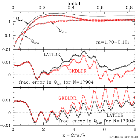
Figure 5: Scattering and absorption for a $m=1.7+0.1i$ sphere, calculated using two prescriptions for the polarizability: LATTDR is the lattice dispersion relation result of Draine & Goodman (1993). GKDLDR is the lattice dispersion relation result of Gutkowicz-Krusin & Draine (2004). We see that there is little practical difference between them for this case. For other examples see Gutkowicz-Krusin & Draine (2004).

Option LATTDR specifies that the “Lattice Dispersion Relation” of Draine & Goodman (1993) be employed to determine the dipole polarizabilities. This polarizability works well.

Option GKDLDR specifies that the polarizability be prescribed by the “Lattice Dispersion Relation”, but with the polarizability found by Gutkowicz-Krusin & Draine (2004), who corrected an error in the analysis of Draine & Goodman (1993). The GKDLDR polarizability differs somewhat from the LATTDR polarizability, but the differences in calculated scattering cross sections are relatively small, as can be seen from Figure 5.

12 Dielectric Functions

12.1 Table Specifying Dielectric Function or Refractive Index

In order to assign the appropriate dipole polarizabilities, DDSCAT 6.1 must be given the dielectric constant of the material (or materials) of which the target of interest is composed. Unless the user wishes to use the dielectric function of either solid or liquid H₂O (see below), this information is supplied to DDSCAT through a table (or tables), read by subroutine DIELEC in file dielec.f, and providing either the complex refractive index $m=n+ik$ or complex dielectric function $\epsilon=\epsilon_{1}+i\epsilon_{2}$ as a function of wavelength $\lambda$. Since $m=\epsilon^{1/2}$, or $\epsilon=m^{2}$, the user must supply either $m$ or $\epsilon$, but not both.

The table formatting is intended to be quite flexible. The first line of the table consists of text, up to 80 characters of which will be read and included in the output to identify the choice of dielectric function. (For the sample problem, it consists of simply the statement m = 1.33 + 0.01i.) The second line consists of 5 integers; either the second and third or the fourth and fifth should be zero.

• The first integer specifies which column the wavelength is stored in.

• The second integer specifies which column Re$(m)$ is stored in.

• The third integer specifies which column Im$(m)$ is stored in.

• The fourth integer specifies which column Re$(\epsilon)$ is stored in.

• The fifth integer specifies which column Im$(\epsilon)$ is stored in.

If the second and third integers are zeros, then DIELEC will read Re$(\epsilon)$ and Im$(\epsilon)$ from the file; if the fourth and fifth integers are zeros, then Re$(m)$ and Im$(m)$ will be read from the file.

The third line of the file is used for column headers, and the data begins in line 4. There must be at least 3 lines of data: even if $\epsilon$ is required at only one wavelength, please supply two additional “dummy” wavelength entries in the table so that the interpolation apparatus will not be confused.

12.2 Multiple Dielectric Functions

For targets composed of more than one material, or composed of anisotropic materials, it is necessary to specify more than one dielectric function. This is accomplished by providing multiple files; one file per dielectric function. The files are identified in ddscat.par. Here is an example for a target consisting of two concentric ellipsoids (see description of target option CONELL in §19.3): the inner ellipsoid consists of material with dielectric function (or refractive index) tabulated in the file diel_1.tab, while the region between the inner ellipsoid and outer ellipsoid has dielectric function (or refractive index) tabulated in the file diel_2.tab. Note that ddscat.par specifies NCOMP (the number of dielectric materials to be 2.

’ =================== Parameter file ===================’
’**** PRELIMINARIES ****’
’NOTORQ’ = CMTORQ*6 (DOTORQ, NOTORQ) -- either do or skip torque calculations
’PBCGST’ = CMDSOL*6 (PBCGST, PETRKP) -- select solution method
’GPFAFT’ = CMETHD*6 (GPFAFT, FFTWJ, CONVEX)
’LATTDR’ = CALPHA*6 (LATTDR, SCLDR)
’NOTBIN’ = CBINFLAG (ALLBIN, ORIBIN, NOTBIN)
’NOTCDF’ = CNETFLAG (ALLCDF, ORICDF, NOTCDF)
’CONELL’ = CSHAPE*6 (FRMFIL,ELLIPS,CYLNDR,RCTNGL,HEXGON,TETRAH,UNICYL,...)
32 24 16 16 12 8 = shape parameters SHPAR1, SHPAR2, SHPAR3, ...
2         = NCOMP = number of dielectric materials
’TABLES’ = CDIEL*6 (TABLES,H2OICE,H2OLIQ; if TABLES, then filenames follow...)
’diel_1.tab’ = name of file containing dielectric function
’diel_2.tab’
’**** CONJUGATE GRADIENT DEFINITIONS ****’
0       = INIT (TO BEGIN WITH |X0> = 0)
1.00e-5 = TOL = MAX ALLOWED (NORM OF |G>=AC|E>-ACA|X>)/(NORM OF AC|E>)
’**** Angular resolution for calculation of <cos>, etc. ****’
0.5     = ETASCA (number of angles is proportional to [(3+x)/ETASCA]^2 )
’**** Wavelengths (micron) ****’
6.283185 6.283185 1 ’INV’ = wavelengths (first,last,how many,how=LIN,INV,LOG)
’**** Effective Radii (micron) **** ’
2 2 1 ’LIN’ = eff. radii (first, last, how many, how=LIN,INV,LOG)
**** Define Incident Polarizations ****’
(0,0) (1.,0.) (0.,0.) = Polarization state e01 (k along x axis)
2 = IORTH  (=1 to do only pol. state e01; =2 to also do orth. pol. state)
1 = IWRKSC (=0 to suppress, =1 to write ".sca" file for each target orient.
’**** Prescribe Target Rotations ****’
0.   0.   1  = BETAMI, BETAMX, NBETA (beta=rotation around a1)
0.  90.   3  = THETMI, THETMX, NTHETA (theta=angle between a1 and k)
0.   0.   1  = PHIMIN, PHIMAX, NPHI (phi=rotation angle of a1 around k)
’**** Specify first IWAV, IRAD, IORI (normally 0 0 0) ****’
0   0   0    = first IWAV, first IRAD, first IORI (0 0 0 to begin fresh)
’**** Select Elements of S_ij Matrix to Print ****’
6       = NSMELTS = number of elements of S_ij to print (not more than 9)
11 12 21 22 31 41       = indices ij of elements to print
’**** Specify Scattered Directions ****’
0.  0. 180. 10 = phi, thetan_min, thetan_max, dtheta (in degrees) for plane A
90. 0. 180. 10 = phi, ... for plane B

12.3 Water Ice or Liquid Water

In the event that the user wishes to compute scattering by targets with the refractive index of either solid or liquid H₂O, we have included two “built-in” dielectric functions. If H2OICE is specified on line 10 of ddscat.par, DDSCAT will use the dielectric function of H₂O ice at T=250K as compiled by Warren (1984). If H2OLIQ is specified on line 10 of ddscat.par, DDSCAT will use the dielectric function for liquid H₂O at T=280K using subroutine REFWAT written by Eric A. Smith. For more information see http://atol.ucsd.edu/$\sim$pflatau/refrtab/index.htm .

13 Choice of FFT Algorithm

One major change in going from DDSCAT.4b to 4c was modification of the code to permit use of the GPFA FFT algorithm developed by Dr. Clive Temperton (1992). In going from DDSCAT 5a10 to 6.0 we introduced a new FFT option: the FFTW package of Frigo and Johnson. DDSCAT 6.1continues to offer Temperton’s GPFA code as an alternative (and quite fast) FFT implementation.

Table 1 is the res.dat file created when run on a 2.0 GHz Intel Xeon system, using the pgf77 compiler:

Table 1: Timings for 3 different 3-d FFT implementations

 CPU time (sec) for different 3-D FFT methods
 Machine=2.0 GHz Xeon, 256kB L2 cache, pgf77 compiler
 parameter LVR = 64
 LVR="length of vector registers" in gpfa2f,gpfa3f,gpfa5f
============================================================
                  Brenner    Temperton Frigo & Johnson
   NX  NY  NZ     (FOURX)     (GPFA)       (FFTW)
   31  31  31       0.040       0.082       0.030
   32  32  32       0.012       0.007       0.004
   34  34  34       0.040       0.120       0.023
   36  36  36       0.047       0.008       0.008
   38  38  38       0.060       0.013       0.037
   40  40  40       0.055       0.013       0.008
   43  43  43       0.155       0.018       0.072
   45  45  45       0.125       0.017       0.014
   47  47  47       0.220       0.023       0.132
   48  48  48       0.120       0.023       0.016
   49  49  49       0.150       0.024       0.019
   50  50  50       0.170       0.024       0.020
   52  52  52       0.180       0.033       0.028
   54  54  54       0.260       0.031       0.023
   57  57  57       0.310       0.042       0.147
   60  60  60       0.320       0.042       0.042
   62  62  62       0.440       0.068       0.210
   64  64  64       0.240       0.068       0.055
   68  68  68       0.470       0.090       0.190
   72  72  72       0.600       0.093       0.060
   74  74  74       0.850       0.093       0.347
   75  75  75       0.730       0.093       0.077
   78  78  78       0.800       0.120       0.090
   80  80  80       0.710       0.120       0.100
   81  81  81       1.070       0.115       0.100
   86  86  86       1.510       0.170       0.630
   90  90  90       1.390       0.170       0.125
   93  93  93       1.740       0.260       0.720
   96  96  96       1.920       0.260       0.270
   98  98  98       1.590       0.230       0.170
  100 100 100       1.670       0.225       0.225
  104 104 104       1.740       0.280       0.220
  108 108 108       2.490       0.280       0.210
  114 114 114       2.940       0.450       1.100
  120 120 120       3.100       0.440       0.380
  123 123 123       4.710       0.440       1.750
  125 125 125       3.640       0.450       0.440
  127 127 127      10.400       0.950       2.000
  128 128 128       3.310       0.960       1.020
  132 132 132       4.140       0.600       0.540
  135 135 135       5.420       0.600       0.510
  140 140 140       4.800       0.920       0.550
  144 144 144       7.150       0.940       0.800
  147 147 147       6.170       0.870       0.690
  150 150 150       6.930       0.870       0.720
  155 155 155       8.350       1.330       3.540
  160 160 160      11.110       1.330       1.640
  161 161 161       8.450       1.110       3.640
  162 162 162      10.190       1.110       0.850
  171 171 171      11.380       1.530       3.770
  180 180 180      12.480       1.540       1.210
  186 186 186      15.920       2.600       6.310
  192 192 192      20.050       2.610       3.110
  196 196 196      14.270       2.500       1.690
  200 200 200      16.180       2.500       1.820

It is clear that both the GPFA code and the FFTW code are much faster than the Brenner FFT (by a factor of 7 for the 100$\times$100$\times$100 case). The FFTW code and GPFA code are quite comparable in performance – for some cases the GPFA code is faster, for other cases the FFTW code is faster. For target dimensions which are factorizable as $2^{i}3^{j}5^{k}$ (for integer $i$, $j$, $k$), the GPFA and FFTW codes have the same memory requirements. For targets with extents $N_{x}$, $N_{y}$, $N_{z}$ which are not factorizable as $2^{i}3^{j}5^{k}$, the GPFA code needs to “extend” the computational volume to have values of $N_{x}$, $N_{y}$, and $N_{z}$ which are factorizable by 2, 3, and 5. For these cases, GPFA requires somewhat more memory than FFTW. However, the fractional difference in required memory is not large, since integers factorizable as $2^{i}3^{j}5^{k}$ occur fairly frequently.

Based on Figure 5, we see that while for some cases FFTW 2.1.5 is faster than the GPFA algorithm, the difference appears to be fairly marginal.

The GPFA code contains a parameter LVR which is set in data statements in the routines gpfa2f, gpfa3f, and gpfa5f. LVR is supposed to be optimized to correspond to the “length of a vector register” on vector machines. As delivered, this parameter is set to 64, which is supposed to be appropriate for Crays other than the C90 (for the C90, 128 is supposed to be preferable). The value of LVR is not critical for scalar machines, as long as it is fairly large. We found little difference between LVR=64 and 128 on a Sparc 10/51, on an Ultrasparc 170, and on an Intel Xeon cpu. You may wish to experiment with different LVR values on your computer architecture. To change LVR, you need to edit gpfa.f and change the three data statements where LVR is set.

The choice of FFT implementation is obtained by specifying one of:

• FFTW21 to use the FFTW 2.1.x algorithm of Frigo and Johnson – this is recommended, but requires that the FFTW 2.1.x library be installed on your system.

• GPFAFT to use the GPFA algorithm (Temperton 1992) – this is almost as fast as the FFTW package, and does not require that the FFTW package be installed on your system;

• CONVEX to use the native FFT routine on a Convex system (this option is presumably obsolete, but is retained as an example of how to use a system-specific native routine).

14 Choice of Iterative Algorithm

As discussed elsewhere (e.g., Draine 1988), the problem of electromagnetic scattering of an incident wave ${\bf E}_{\rm inc}$ by an array of $N$ point dipoles can be cast in the form

$${\bf A}{\bf P}={\bf E}$$ (17)

where ${\bf E}$ is a $3N$-dimensional (complex) vector of the incident electric field ${\bf E}_{\rm inc}$ at the $N$ lattice sites, ${\bf P}$ is a $3N$-dimensional (complex) vector of the (unknown) dipole polarizations, and ${\bf A}$ is a $3N\times 3N$ complex matrix.

Because $3N$ is a large number, direct methods for solving this system of equations for the unknown vector ${\bf P}$ are impractical, but iterative methods are useful: we begin with a guess (typically, ${\bf P}=0$) for the unknown polarization vector, and then iteratively improve the estimate for ${\bf P}$ until equation (17) is solved to some error criterion. The error tolerance may be specified as

$${|{\bf A}^{\dagger}{\bf A}{\bf P}-{\bf A}^{\dagger}{\bf E}|\over|{\bf A}^{\dagger}{\bf E}|}<h~{}~{}~{},$$ (18)

where ${\bf A}^{\dagger}$ is the Hermitian conjugate of ${\bf A}$ [$(A^{\dagger})_{ij}\equiv(A_{ji})^{*}$], and $h$ is the error tolerance. We typically use $h=10^{-5}$ in order to satisfy eq.(17) to high accuracy. The error tolerance $h$ can be specified by the user through the parameter TOL in the parameter file ddscat.par (see Appendix A).

A major change in going from DDSCAT.4b to 5a (and subsequent versions) was the implementation of several different algorithms for iterative solution of the system of complex linear equations. DDSCAT 6.1 is now structured to permit solution algorithms to be treated in a fairly “modular” fashion, facilitating the testing of different algorithms. Many algorithms were compared by Flatau (1997); two of them performed well and are made available to the user in DDSCAT 6.1. The choice of algorithm is made by specifying one of the options:

• PBCGST – Preconditioned BiConjugate Gradient with STabilitization method from the Parallel Iterative Methods (PIM) package created by R. Dias da Cunha and T. Hopkins.

• PETRKP – the complex conjugate gradient algorithm of Petravic & Kuo-Petravic (1979), as coded in the Complex Conjugate Gradient package (CCGPACK) created by P.J. Flatau. This is the algorithm discussed by Draine (1988) and used in previous versions of DDSCAT.

Both methods work well. Our experience suggests that PBCGST is often faster than PETRKP, by perhaps a factor of two. We therefore recommend it, but include the PETRKP method as an alternative.

The Parallel Iterative Methods (PIM) by Rudnei Dias da Cunha (rdd@ukc.ac.uk) and Tim Hopkins (trh@ukc.ac.uk) is a collection of Fortran 77 routines designed to solve systems of linear equations on parallel and scalar computers using a variety of iterative methods (available at http://www.mat.ufrgs.br/pim-e.html). PIM offers a number of iterative methods, including

• Conjugate-Gradients, CG (Hestenes 1952),

• Bi-Conjugate-Gradients, BICG (Fletcher 1976),

• Conjugate-Gradients squared, CGS (Sonneveld 1989),

• the stabilised version of Bi-Conjugate-Gradients, BICGSTAB (van der Vorst 1991),

• the restarted version of BICGSTAB, RBICGSTAB (Sleijpen & Fokkema 1992)

• the restarted generalized minimal residual, RGMRES (Saad 1986),

• the restarted generalized conjugate residual, RGCR (Eisenstat 1983),

• the normal equation solvers, CGNR (Hestenes 1952 and CGNE (Craig 1955),

• the quasi-minimal residual, QMR (highly parallel version due to Bucker & Sauren 1996),

• transpose-free quasi-minimal residual, TFQMR (Freund 1992),

• the Chebyshev acceleration, CHEBYSHEV (Young 1981).

The source code for these methods is distributed with DDSCAT but only PBCGST and PETRKP can be called directly via ddscat.par. It is possible to add other options by changing the code in getfml.f . Flatau (1997) has compared the convergence rates of a number of different methods.

A helpful introduction to conjugate gradient methods is provided by the report “Conjugate Gradient Method Without Agonizing Pain” by Jonathan R. Shewchuk.

15 Calculation of $\langle\cos\theta\rangle$, Radiative Force, and Radiation Torque

In addition to solving the scattering problem for a dipole array, DDSCAT 6.1 can compute the three-dimensional force ${\bf F}_{\rm rad}$ and torque ${\bf\Gamma}_{\rm rad}$ exerted on this array by the incident and scattered radiation fields. The radiation torque calculation is carried out, after solving the scattering problem, only if DOTORQ has been specified in ddscat.par. For each incident polarization mode, the results are given in terms of dimensionless efficiency vectors ${\bf Q}_{pr}$ and ${\bf Q}_{\Gamma}$, defined by

$${\bf Q}_{pr}\equiv{{\bf F}_{\rm rad}\over\pi a_{\rm eff}^{2}u_{\rm rad}}~{}~{}~{},$$ (19)

$${\bf Q}_{\Gamma}\equiv{k{\bf\Gamma}_{\rm rad}\over\pi a_{\rm eff}^{2}u_{\rm rad}}~{}~{}~{},$$ (20)

where ${\bf F}_{\rm rad}$ and ${\bf\Gamma}_{\rm rad}$ are the time-averaged force and torque on the dipole array, $k=2\pi/\lambda$ is the wavenumber in vacuo, and $u_{\rm rad}=E_{0}^{2}/8\pi$ is the time-averaged energy density for an incident plane wave with amplitude $E_{0}\cos(\omega t+\phi)$. The radiation pressure efficiency vector can be written

$${\bf Q}_{\rm pr}=Q_{\rm ext}{\hat{\bf k}}-Q_{\rm sca}{\bf g}~{}~{}~{},$$ (21)

where ${\hat{\bf k}}$ is the direction of propagation of the incident radiation, and the vector g is the mean direction of propagation of the scattered radiation:

$${\bf g}={1\over C_{\rm sca}}\int d\Omega{dC_{\rm sca}({\hat{\bf n}},{\hat{\bf k}})\over d\Omega}{\hat{\bf n}}~{}~{}~{},$$ (22)

where $d\Omega$ is the element of solid angle in scattering direction ${\hat{\bf n}}$, and $dC_{\rm sca}/d\Omega$ is the differential scattering cross section.

Equations for the evaluation of the radiative force and torque are derived by Draine & Weingartner (1996). It is important to note that evaluation of ${\bf Q}_{pr}$ and ${\bf Q}_{\Gamma}$ involves averaging over scattering directions to evaluate the linear and angular momentum transport by the scattered wave. This evaluation requires appropriate choices of the parameter ETASCA – see §22.

In addition, DDSCAT 6.1 calculates $\langle\cos\theta\rangle$ [the first component of the vector $g$ in eq. (22)] and the second moment $\langle\cos^{2}\theta\rangle$. These two moments are useful measures of the anisotropy of the scattering. For example, Draine (2003) gives an analytic approximation to the scattering phase function of dust mixtures that is parameterized by the two moments $\langle\cos\theta\rangle$ and $\langle\cos^{2}\theta\rangle$.

16 Memory Requirements

Since Fortran-77 does not allow for dynamic memory allocation, the executable has compiled into it the dimensions for a number of arrays; these array dimensions limit the size of the dipole array which the code can handle. The source code supplied to you (which can be used to run the sample calculation with 12288 dipoles) is restricted to problems with targets with a maximum extent of 32 lattice spacings along the $x$-, $y$-, and $z$-directions (MXNX=32,MXNY=32,MXNZ=32; i.e, the target must fit within an 32$\times$32$\times$32=32768 cube) and involve at most 9 different dielectric functions (MXCOMP=9). With this dimensioning, the executable requires about 1.3 MB of memory to run on an Ultrasparc system; memory requirements on other hardware and with other compilers should be similar. To run larger problems, you will need to edit the DDSCAT.f to change certain PARAMETER values and then recompile.

All of the dimensioning takes place in the main program DDSCAT – this should be the only routine which it is necessary to recompile. All of the dimensional parameters are set in PARAMETER statements appearing before the array declarations. You need simply edit the parameter statements. Remember, of course, that the amount of memory allocated by the code when it runs will depend upon these dimensioning parameters, so do not set them to ridiculously large values! The parameters MXNX, MXNY, MXNZ specify the maximum extent of the target in the $x$-, $y$-, or $z$-directions. The parameter MXCOMP specifies the maximum number of different dielectric functions which the code can handle at one time. The comment statements in the code supply all the information you should need to change these parameters.

The memory requirement for DDSCAT 6.1 (with the netCDF and FFTW options disabled) is approximately

$$(1690+0.764{\tt MXNX}\times{\tt MXNY}\times{\tt MXNZ}){\rm~{}kbytes}$$ (23)

Thus a 32$\times$32$\times$32 calculation requires 22.5 MBytes, while a 48$\times$48$\times$48 calculation requires 73.0 MBytes. These values are for the pgf77 compiler on an Intel Xeon system running the Linux operating system.

17 Target Orientation

Recall that we define a “Lab Frame” (LF) in which the incident radiation propagates in the $+x$ direction. In ddscat.par one specifies the first polarization state ${\hat{\bf e}}_{01}$ (which obviously must lie in the $y,z$ plane in the LF); DDSCAT automatically constructs a second polarization state ${\hat{\bf e}}_{02}={\hat{\bf x}}\times{\hat{\bf e}}_{01}^{*}$ orthogonal to ${\hat{\bf e}}_{01}$ (here ${\hat{\bf x}}$ is the unit vector in the $+x$ direction of the LF. For purposes of discussion we will always let unit vectors ${\hat{\bf x}}$, ${\hat{\bf y}}$, ${\hat{\bf z}}={\hat{\bf x}}\times{\hat{\bf y}}$ be the three coordinate axes of the LF. Users will often find it convenient to let polarization vectors ${\hat{\bf e}}_{01}={\hat{\bf y}}$, ${\hat{\bf e}}_{02}={\hat{\bf z}}$ (although this is not mandatory – see §21).

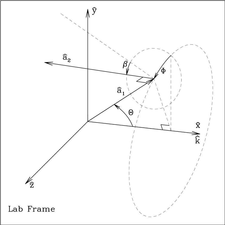
Figure 7: Target orientation in the Lab Frame. ${\hat{\bf x}}$ is the direction of propagation of the incident radiation, and ${\hat{\bf y}}$ is the direction of the “real” component of the first incident polarization mode. In this coordinate system, the orientation of target axis ${\hat{\bf a}}_{1}$ is specified by angles $\Theta$ and $\Phi$. With target axis ${\hat{\bf a}}_{1}$ fixed, the orientation of target axis ${\hat{\bf a}}_{2}$ is then determined by angle $\beta$ specifying rotation of the target around ${\hat{\bf a}}_{1}$. When $\beta=0$, ${\hat{\bf a}}_{2}$ lies in the ${\hat{\bf a}}_{1}$,${\hat{\bf x}}$ plane.

Recall that definition of a target involves specifying two unit vectors, ${\hat{\bf a}}_{1}$ and ${\hat{\bf a}}_{2}$, which are imagined to be “frozen” into the target. We require ${\hat{\bf a}}_{2}$ to be orthogonal to ${\hat{\bf a}}_{1}$. Therefore we may define a “Target Frame” (TF) defined by the three unit vectors ${\hat{\bf a}}_{1}$, ${\hat{\bf a}}_{2}$, and ${\hat{\bf a}}_{3}={\hat{\bf a}}_{1}\times{\hat{\bf a}}_{2}$ .

For example, when DDSCAT creates a 32$\times$24$\times$16 rectangular solid, it fixes ${\hat{\bf a}}_{1}$ to be along the longest dimension of the solid, and ${\hat{\bf a}}_{2}$ to be along the next-longest dimension.

Orientation of the target relative to the incident radiation can in principle be determined two ways:

1. specifying the direction of ${\hat{\bf a}}_{1}$ and ${\hat{\bf a}}_{2}$ in the LF, or

2. specifying the directions of ${\hat{\bf x}}$ (incidence direction) and ${\hat{\bf y}}$ in the TF.

DDSCAT 6.1 uses method 1.: the angles $\Theta$, $\Phi$, and $\beta$ are specified in the file ddscat.par. The target is oriented such that the polar angles $\Theta$ and $\Phi$ specify the direction of ${\hat{\bf a}}_{1}$ relative to the incident direction ${\hat{\bf x}}$, where the ${\hat{\bf x}}$,${\hat{\bf y}}$ plane has $\Phi=0$. Once the direction of ${\hat{\bf a}}_{1}$ is specified, the angle $\beta$ than specifies how the target is to rotated around the axis ${\hat{\bf a}}_{1}$ to fully specify its orientation. A more extended and precise explanation follows:

17.1 Orientation of the Target in the Lab Frame

DDSCAT uses three angles, $\Theta$, $\Phi$, and $\beta$, to specify the directions of unit vectors ${\hat{\bf a}}_{1}$ and ${\hat{\bf a}}_{2}$ in the LF (see Fig. 7).

$\Theta$ is the angle between ${\hat{\bf a}}_{1}$ and ${\hat{\bf x}}$.

When $\Phi=0$, ${\hat{\bf a}}_{1}$ will lie in the ${\hat{\bf x}},{\hat{\bf y}}$ plane. When $\Phi$ is nonzero, it will refer to the rotation of ${\hat{\bf a}}_{1}$ around ${\hat{\bf x}}$: e.g., $\Phi=90^{\circ}$ puts ${\hat{\bf a}}_{1}$ in the ${\hat{\bf x}},{\hat{\bf z}}$ plane.

When $\beta=0$, ${\hat{\bf a}}_{2}$ will lie in the ${\hat{\bf x}},{\hat{\bf a}}_{1}$ plane, in such a way that when $\Theta=0$ and $\Phi=0$, ${\hat{\bf a}}_{2}$ is in the ${\hat{\bf y}}$ direction: e.g, $\Theta=90^{\circ}$, $\Phi=0$, $\beta=0$ has ${\hat{\bf a}}_{1}={\hat{\bf y}}$ and ${\hat{\bf a}}_{2}=-{\hat{\bf x}}$. Nonzero $\beta$ introduces an additional rotation of ${\hat{\bf a}}_{2}$ around ${\hat{\bf a}}_{1}$: e.g., $\Theta=90^{\circ}$, $\Phi=0$, $\beta=90^{\circ}$ has ${\hat{\bf a}}_{1}={\hat{\bf y}}$ and ${\hat{\bf a}}_{2}={\hat{\bf z}}$.

Mathematically:

$${\hat{\bf a}}_{1} = {\hat{\bf x}}\cos\Theta+{\hat{\bf y}}\sin\Theta\cos\Phi+{\hat{\bf z}}\sin\Theta\sin\Phi$$ (24)

$${\hat{\bf a}}_{2} = -{\hat{\bf x}}\sin\Theta\cos\beta+{\hat{\bf y}}[\cos\Theta\cos\beta\cos\Phi-\sin\beta\sin\Phi]$$ (25)

$$+{\hat{\bf z}}[\cos\Theta\cos\beta\sin\Phi+\sin\beta\cos\Phi]$$

$${\hat{\bf a}}_{3} = {\hat{\bf x}}\sin\Theta\sin\beta-{\hat{\bf y}}[\cos\Theta\sin\beta\cos\Phi+\cos\beta\sin\Phi]$$ (26)

$$-{\hat{\bf z}}[\cos\Theta\sin\beta\sin\Phi-\cos\beta\cos\Phi]$$

or, equivalently:

$${\hat{\bf x}} = {\hat{\bf a}}_{1}\cos\Theta-{\hat{\bf a}}_{2}\sin\Theta\cos\beta+{\hat{\bf a}}_{3}\sin\Theta\sin\beta$$ (27)

$${\hat{\bf y}} = {\hat{\bf a}}_{1}\sin\Theta\cos\Phi+{\hat{\bf a}}_{2}[\cos\Theta\cos\beta\cos\Phi-\sin\beta\sin\Phi]$$ (28)

$$-{\hat{\bf a}}_{3}[\cos\Theta\sin\beta\cos\Phi+\cos\beta\sin\Phi]$$

$${\hat{\bf z}} = {\hat{\bf a}}_{1}\sin\Theta\sin\Phi+{\hat{\bf a}}_{2}[\cos\Theta\cos\beta\sin\Phi+\sin\beta\cos\Phi]$$ (29)

$$-{\hat{\bf a}}_{3}[\cos\Theta\sin\beta\sin\Phi-\cos\beta\cos\Phi]$$

17.2 Orientation of the Incident Beam in the Target Frame

Under some circumstances, one may wish to specify the target orientation such that ${\hat{\bf x}}$ (the direction of propagation of the radiation) and ${\hat{\bf y}}$ (usually the first polarization direction) and ${\hat{\bf z}}$ (= ${\hat{\bf x}}\times{\hat{\bf y}})$ refer to certain directions in the TF. Given the definitions of the LF and TF above, this is simply an exercise in coordinate transformation. For example, one might wish to have the incident radiation propagating along the (1,1,1) direction in the TF (example 14 below). Here we provide some selected examples:

1. ${\hat{\bf x}}={\hat{\bf a}}_{1}$, ${\hat{\bf y}}={\hat{\bf a}}_{2}$, ${\hat{\bf z}}={\hat{\bf a}}_{3}$ : $\Theta=0$, $\Phi+\beta=0$

2. ${\hat{\bf x}}={\hat{\bf a}}_{1}$, ${\hat{\bf y}}={\hat{\bf a}}_{3}$, ${\hat{\bf z}}=-{\hat{\bf a}}_{2}$ : $\Theta=0$, $\Phi+\beta=90^{\circ}$

3. ${\hat{\bf x}}={\hat{\bf a}}_{2}$, ${\hat{\bf y}}={\hat{\bf a}}_{1}$, ${\hat{\bf z}}=-{\hat{\bf a}}_{3}$ : $\Theta=90^{\circ}$, $\beta=180^{\circ}$, $\Phi=0$

4. ${\hat{\bf x}}={\hat{\bf a}}_{2}$, ${\hat{\bf y}}={\hat{\bf a}}_{3}$, ${\hat{\bf z}}={\hat{\bf a}}_{1}$ : $\Theta=90^{\circ}$, $\beta=180^{\circ}$, $\Phi=90^{\circ}$

5. ${\hat{\bf x}}={\hat{\bf a}}_{3}$, ${\hat{\bf y}}={\hat{\bf a}}_{1}$, ${\hat{\bf z}}={\hat{\bf a}}_{2}$ : $\Theta=90^{\circ}$, $\beta=-90^{\circ}$, $\Phi=0$

6. ${\hat{\bf x}}={\hat{\bf a}}_{3}$, ${\hat{\bf y}}={\hat{\bf a}}_{2}$, ${\hat{\bf z}}=-{\hat{\bf a}}_{1}$ : $\Theta=90^{\circ}$, $\beta=-90^{\circ}$, $\Phi=-90^{\circ}$

7. ${\hat{\bf x}}=-{\hat{\bf a}}_{1}$, ${\hat{\bf y}}={\hat{\bf a}}_{2}$, ${\hat{\bf z}}=-{\hat{\bf a}}_{3}$ : $\Theta=180^{\circ}$, $\beta+\Phi=180^{\circ}$

8. ${\hat{\bf x}}=-{\hat{\bf a}}_{1}$, ${\hat{\bf y}}={\hat{\bf a}}_{3}$, ${\hat{\bf z}}={\hat{\bf a}}_{2}$ : $\Theta=180^{\circ}$, $\beta+\Phi=90^{\circ}$

9. ${\hat{\bf x}}=-{\hat{\bf a}}_{2}$, ${\hat{\bf y}}={\hat{\bf a}}_{1}$, ${\hat{\bf z}}={\hat{\bf a}}_{3}$ : $\Theta=90^{\circ}$, $\beta=0$, $\Phi=0$

10. ${\hat{\bf x}}=-{\hat{\bf a}}_{2}$, ${\hat{\bf y}}={\hat{\bf a}}_{3}$, ${\hat{\bf z}}=-{\hat{\bf a}}_{1}$ : $\Theta=90^{\circ}$, $\beta=0$, $\Phi=-90^{\circ}$

11. ${\hat{\bf x}}=-{\hat{\bf a}}_{3}$, ${\hat{\bf y}}={\hat{\bf a}}_{1}$, ${\hat{\bf z}}=-{\hat{\bf a}}_{2}$ : $\Theta=90^{\circ}$, $\beta=-90^{\circ}$, $\Phi=0$

12. ${\hat{\bf x}}=-{\hat{\bf a}}_{3}$, ${\hat{\bf y}}={\hat{\bf a}}_{2}$, ${\hat{\bf z}}={\hat{\bf a}}_{1}$ : $\Theta=90^{\circ}$, $\beta=-90^{\circ}$, $\Phi=90^{\circ}$

13. ${\hat{\bf x}}=({\hat{\bf a}}_{1}+{\hat{\bf a}}_{2})/\surd 2$, ${\hat{\bf y}}={\hat{\bf a}}_{3}$, ${\hat{\bf z}}=({\hat{\bf a}}_{1}-{\hat{\bf a}}_{2})/\surd 2$: $\Theta=45^{\circ}$, $\beta=180^{\circ}$, $\Phi=90^{\circ}$

14. ${\hat{\bf x}}=({\hat{\bf a}}_{1}+{\hat{\bf a}}_{2}+{\hat{\bf a}}_{3})/\surd 3$, ${\hat{\bf y}}=({\hat{\bf a}}_{1}-{\hat{\bf a}}_{2})/\surd 2$, ${\hat{\bf z}}=({\hat{\bf a}}_{1}+{\hat{\bf a}}_{2}-2{\hat{\bf a}}_{3})/\surd 6$: $\Theta=54.7356^{\circ}$, $\beta=135^{\circ}$, $\Phi=30^{\circ}$.

17.3 Sampling in $\Theta$, $\Phi$, and $\beta$

The present version, DDSCAT 6.1, chooses the angles $\beta$, $\Theta$, and $\Phi$ to sample the intervals (BETAMI,BETAMX), (THETMI,THETMX), (PHIMIN,PHIMAX), where BETAMI, BETAMX, THETMI, THETMX, PHIMIN, PHIMAX are specified in ddscat.par . The prescription for choosing the angles is to:

• uniformly sample in $\beta$;

• uniformly sample in $\Phi$;

• uniformly sample in $\cos\Theta$.

This prescription is appropriate for random orientation of the target, within the specified limits of $\beta$, $\Phi$, and $\Theta$.

Note that when DDSCAT 6.1 chooses angles it handles $\beta$ and $\Phi$ differently from $\Theta$. The range for $\beta$ is divided into NBETA intervals, and the midpoint of each interval is taken. Thus, if you take BETAMI=0, BETAMX=90, NBETA=2 you will get $\beta=22.5^{\circ}$ and $67.5^{\circ}$. Similarly, if you take PHIMIN=0, PHIMAX=180, NPHI=2 you will get $\Phi=45^{\circ}$ and $135^{\circ}$.

Sampling in $\Theta$ is done quite differently from sampling in $\beta$ and $\Phi$. First, as already mentioned above, DDSCAT 6.1 samples uniformly in $\cos\Theta$, not $\Theta$. Secondly, the sampling depends on whether NTHETA is even or odd.

• If NTHETA is odd, then the values of $\Theta$ selected include the extreme values THETMI and THETMX; thus, THETMI=0, THETMX=90, NTHETA=3 will give you $\Theta=0,60^{\circ},90^{\circ}$.

• If NTHETA is even, then the range of $\cos\Theta$ will be divided into NTHETA intervals, and the midpoint of each interval will be taken; thus, THETMI=0, THETMX=90, NTHETA=2 will give you $\Theta=41.41^{\circ}$ and $75.52^{\circ}$ [$\cos\Theta=0.25$ and $0.75$].

The reason for this is that if odd NTHETA is specified, than the “integration” over $\cos\Theta$ is performed using Simpson’s rule for greater accuracy. If even NTHETA is specified, then the integration over $\cos\Theta$ is performed by simply taking the average of the results for the different $\Theta$ values.

If averaging over orientations is desired, it is recommended that the user specify an odd value of NTHETA so that Simpson’s rule will be employed.

18 Orientational Averaging

DDSCAT has been constructed to facilitate the computation of orientational averages. How to go about this depends on the distribution of orientations which is applicable.

18.1 Randomly-Oriented Targets

For randomly-oriented targets, we wish to compute the orientational average of a quantity $Q(\beta,\Theta,\Phi)$:

$$\langle Q\rangle={1\over 8\pi^{2}}\int_{0}^{2\pi}d\beta\int_{-1}^{1}d\cos\Theta\int_{0}^{2\pi}d\Phi~{}Q(\beta,\Theta,\Phi)~{}~{}~{}.$$ (30)

To compute such averages, all you need to do is edit the file ddscat.par so that DDSCAT knows what ranges of the angles $\beta$, $\Theta$, and $\Phi$ are of interest. For a randomly-oriented target with no symmetry, you would need to let $\beta$ run from 0 to $360^{\circ}$, $\Theta$ from 0 to $180^{\circ}$, and $\Phi$ from 0 to $360^{\circ}$.

For targets with symmetry, on the other hand, the ranges of $\beta$, $\Theta$, and $\Phi$ may be reduced. First of all, remember that averaging over $\Phi$ is relatively “inexpensive”, so when in doubt average over 0 to $360^{\circ}$; most of the computational “cost” is associated with the number of different values of ($\beta$,$\Theta$) which are used. Consider a cube, for example, with axis ${\hat{\bf a}}_{1}$ normal to one of the cube faces; for this cube $\beta$ need run only from 0 to $90^{\circ}$, since the cube has fourfold symmetry for rotations around the axis ${\hat{\bf a}}_{1}$. Furthermore, the angle $\Theta$ need run only from 0 to $90^{\circ}$, since the orientation ($\beta$,$\Theta$,$\Phi$) is indistinguishable from ($\beta$, $180^{\circ}-\Theta$, $360^{\circ}-\Phi$).

For targets with symmetry, the user is encouraged to test the significance of $\beta$,$\Theta$,$\Phi$ on targets with small numbers of dipoles (say, of the order of 100 or so) but having the desired symmetry.

It is important to remember that DDSCAT.4b handled even and odd values of NTHETA differently – see §8 above! For averaging over random orientations odd values of NTHETA are to be preferred, as this will allow use of Simpson’s rule in evaluating the “integral” over $\cos\Theta$.

18.2 Nonrandomly-Oriented Targets

Some special cases (where the target orientation distribution is uniform for rotations around the $x$ axis = direction of propagation of the incident radiation), one may be able to use DDSCAT 6.1 with appropriate choices of input parameters. More generally, however, you will need to modify subroutine ORIENT to generate a list of NBETA values of $\beta$, NTHETA values of $\Theta$, and NPHI values of $\Phi$, plus two weighting arrays WGTA(1-NTHETA,1-NPHI) and WGTB(1-NBETA). Here WGTA gives the weights which should be attached to each ($\Theta$,$\Phi$) orientation, and WGTB gives the weight to be attached to each $\beta$ orientation. Thus each orientation of the target is to be weighted by the factor WGTA$\times$WGTB. For the case of random orientations, DDSCAT 6.1 chooses $\Theta$ values which are uniformly spaced in $\cos\Theta$, and $\beta$ and $\Phi$ values which are uniformly spaced, and therefore uses uniform weights WGTB=1./NBETA

When NTHETA is even, DDSCAT sets WGTA=1./(NTHETA$\times$NPHI)

but when NTHETA is odd, DDSCAT uses Simpson’s rule when integrating over $\Theta$ and WGTA= (1/3 or 4/3 or 2/3)/(NTHETA$\times$NPHI)

Note that the program structure of DDSCAT may not be ideally suited for certain highly oriented cases. If, for example, the orientation is such that for a given $\Phi$ value only one $\Theta$ value is possible (this situation might describe ice needles oriented with the long axis perpendicular to the vertical in the Earth’s atmosphere, illuminated by the Sun at other than the zenith) then it is foolish to consider all the combinations of $\Theta$ and $\Phi$ which the present version of DDSCAT is set up to do. We hope to improve this in a future version of DDSCAT.

19 Target Generation

DDSCAT contains routines to generate dipole arrays representing targets of various geometries, including spheres, ellipsoids, rectangular solids, cylinders, hexagonal prisms, tetrahedra, two touching ellipsoids, and three touching ellipsoids.

The target type is specified by variable CSHAPE on line 9 of ddscat.par, and the target dimensions (in units of interdipole spacing $d$) is specified by up to 6 target shape parameters (SHPAR1, SHPAR2, SHPAR3, …) on line 10.

The target geometry is most conveniently described in a coordinate system attached to the target which we refer to as the “Target Frame” (TF), so in this section only we will let x,y,z be coordinates in the Target Frame. Once the target is generated, the orientation of the target in the Lab Frame is accomplished as described in §17.

Target geometries currently supported include:

19.1 ELLIPS = Homogeneous, isotropic ellipsoid.

“Lengths” SHPAR1, SHPAR2, SHPAR3 in the $x$, $y$, $z$ directions in the TF. $(x/{\tt SHPAR1})^{2}+(y/{\tt SHPAR2})^{2}+(z/{\tt SHPAR3})^{2}=d^{2}/4$, where $d$ is the interdipole spacing.
The target axes are set to ${\hat{\bf a}}_{1}=(1,0,0)$ and ${\hat{\bf a}}_{2}=(0,1,0)$ in the TF.
User must set NCOMP=1 on line 9 of ddscat.par.
A homogeneous, isotropic sphere is obtained by setting SHPAR1 = SHPAR2 = SHPAR3 = diameter/$d$.

19.2 ANIELL = Homogeneous, anisotropic ellipsoid.

SHPAR1, SHPAR2, SHPAR3 have same meaning as for ELLIPS. Target axes ${\hat{\bf a}}_{1}=(1,0,0)$ and ${\hat{\bf a}}_{2}=(0,1,0)$ in the TF. It is assumed that the dielectric tensor is diagonal in the TF. User must set NCOMP=3 and provide $xx$, $yy$, $zz$ elements of the dielectric tensor.

19.3 CONELL = Two concentric ellipsoids

SHPAR1, SHPAR2, SHPAR3 specify the lengths along $x$, $y$, $z$ axes (in the TF) of the outer ellipsoid; SHPAR4, SHPAR5, SHPAR6 are the lengths, along the $x$, $y$, $z$ axes (in the TF) of the inner ellipsoid. The “core” within the inner ellipsoid is composed of isotropic material 1; the “mantle” between inner and outer ellipsoids is composed of isotropic material 2. Target axes ${\hat{\bf a}}_{1}=(1,0,0)$, ${\hat{\bf a}}_{2}=(0,1,0)$ in TF. User must set NCOMP=2 and provide dielectric functions for “core” and “mantle” materials.

19.4 CYLNDR = Homogeneous, isotropic cylinder

Length/$d$=SHPAR1, diameter/$d$=SHPAR2, with cylinder axis $={\hat{\bf a}}_{1}=(1,0,0)$ and ${\hat{\bf a}}_{2}=(0,1,0)$ in the TF. User must set NCOMP=1.

19.5 CYLCAP = Homogeneous, isotropic cylinder with hemispherical end-caps

Cylinder length (not including caps!)/$d$=SHPAR1, diameter/$d$=SHPAR2, with cylinder axis $={\hat{\bf a}}_{1}=(1,0,0)$ and ${\hat{\bf a}}_{2}=(0,1,0)$ in the TF. Note that the target length (including end-caps) will be (SHPAR1 + SHPAR2)$\times d$. User must set NCOMP=1.

19.6 UNICYL = Homogeneous cylinder with unixial anisotropic dielectric tensor

SHPAR1, SHPAR2 have same meaning as for CYLNDR. Cylinder axis $={\hat{\bf a}}_{1}=(1,0,0)$, ${\hat{\bf a}}_{2}=(0,1,0)$. It is assumed that the dielectric tensor $\epsilon$ is diagonal in the TF, with $\epsilon_{yy}=\epsilon_{zz}$. User must set NCOMP=2. Dielectric function 1 is for ${\bf E}\parallel{\bf\hat{a}}_{1}$ (cylinder axis), dielectric function 2 is for ${\bf E}\perp{\bf\hat{a}}_{1}$.

19.7 RCTNGL = Homogeneous, isotropic, rectangular solid

x, y, z lengths/$d$ = SHPAR1, SHPAR2, SHPAR3. Target axes ${\hat{\bf a}}_{1}=(1,0,0)$ and ${\hat{\bf a}}_{2}=(0,1,0)$ in the TF. User must set NCOMP=1.

19.8 ANIREC = Homogeneous, anisotropic, rectangular solid

x, y, z lengths/$d$ = SHPAR1, SHPAR2, SHPAR3. Target axes ${\hat{\bf a}}_{1}=(1,0,0)$ and ${\hat{\bf a}}_{2}=(0,1,0)$ in the TF. Dielectric tensor is assumed to be diagonal in the target frame. User must set NCOMP=3 and supply names of three files for $\epsilon$ as a function of wavelength or energy: first for $\epsilon_{xx}$, second for $\epsilon_{yy}$, and third for $\epsilon_{zz}$, as in the following sample ddscat.par file:

’ =================== Parameter file ===================’
’**** PRELIMINARIES ****’
’NOTORQ’= CMTORQ*6 (DOTORQ, NOTORQ) -- either do or skip torque calculations
’PBCGST’= CMDSOL*6 (PBCGST, PETRKP) -- select solution method
’GPFAFT’= CMETHD*6 (GPFAFT, FFTW21, CONVEX)
’LATTDR’= CALPHA*6 (LATTDR is only supported option now)
’NOTBIN’= CBINFLAG (ALLBIN, ORIBIN, NOTBIN)
’NOTCDF’= CNETFLAG (ALLCDF, ORICDF, NOTCDF)
’ANIREC’= CSHAPE*6 (FRMFIL,ELLIPS,CYLNDR,RCTNGL,HEXGON,TETRAH,UNICYL,...)
10 25 50 = shape parameters PAR1, PAR2, PAR3
3         = NCOMP = number of dielectric materials
’TABLES’= CDIEL*6 (TABLES,H2OICE,H2OLIQ; if TABLES, then filenames follow...)
’/u/draine/DDA/diel/m2.00_0.10’ = name of file containing dielectric function
’/u/draine/DDA/diel/m1.50_0.00’
’/u/draine/DDA/diel/m1.50_0.00’
’**** CONJUGATE GRADIENT DEFINITIONS ****’
0       = INIT (TO BEGIN WITH |X0> = 0)
1.00e-5 = ERR = MAX ALLOWED (NORM OF |G>=AC|E>-ACA|X>)/(NORM OF AC|E>)
’**** Angular resolution for calculation of <cos>, etc. ****’
2.0     = ETASCA (number of angles is proportional to [(2+x)/ETASCA]^2 )
’**** Wavelengths (micron) ****’
500. 500. 1 ’INV’ = wavelengths (first,last,how many,how=LIN,INV,LOG)
’**** Effective Radii (micron) **** ’
30.60 30.60 1  ’LIN’ = eff. radii (first, last, how many, how=LIN,INV,LOG)
’**** Define Incident Polarizations ****’
(0,0) (1.,0.) (0.,0.) = Polarization state e01 (k along x axis)
2 = IORTH  (=1 to do only pol. state e01; =2 to also do orth. pol. state)
1 = IWRKSC (=0 to suppress, =1 to write ".sca" file for each target orient.
’**** Prescribe Target Rotations ****’
 0.   0.  1  = BETAMI, BETAMX, NBETA (beta=rotation around a1)
 0.  90.  3  = THETMI, THETMX, NTHETA (theta=angle between a1 and k)
 0.   0.  1  = PHIMIN, PHIMAX, NPHI (phi=rotation angle of a1 around k)
’**** Specify first IWAV, IRAD, IORI (normally 0 0 0) ****’
0   0   0    = first IWAV, first IRAD, first IORI (0 0 0 to begin fresh)
’**** Select Elements of S_ij Matrix to Print ****’
6       = NSMELTS = number of elements of S_ij to print (not more than 9)
11 12 21 22 31 41       = indices ij of elements to print
’**** Specify Scattered Directions ****’
0.  0. 180. 30 = phi, thetan_min, thetan_max, dtheta (in degrees) for plane A
90. 0. 180. 30 = phi, ... for plane B

19.9 HEXGON = Homogeneous, isotropic hexagonal prism

SHPAR1 = (Length of prism)/$d$ = (distance between hexagonal faces)/$d$, SHPAR2 = (distance between opposite vertices of one hexagonal face)/$d$ = 2$\times$hexagon side/$d$. Note that Target axis ${\hat{\bf a}}_{1}=(1,0,0)$ in the TF is along the prism axis, and target axis ${\hat{\bf a}}_{2}=(0,1,0)$ in the TF is normal to one of the rectangular faces of the hexagonal prism. User must set NCOMP=1.

19.10 TETRAH = Homogeneous, isotropic tetrahedron

SHPAR1=length/$d$ of one edge. Orientation: one face parallel to $y$,$z$ plane (in the TF), opposite “vertex” is in $+x$ direction, and one edge is parallel to $z$ axis (in the TF). Target axes ${\hat{\bf a}}_{1}=(1,0,0)$ [emerging from one vertex] and ${\hat{\bf a}}_{2}=(0,1,0)$ [emerging from an edge] in the TF. User must set NCOMP=1.

19.11 TWOSPH = Two touching homogeneous, isotropic spheroids, with distinct compositions

First spheroid has length SHPAR1 along symmetry axis, diameter SHPAR2 perpendicular to symmetry axis. Second spheroid has length SHPAR3 along symmetry axis, diameter SHPAR4 perpendicular to symmetry axis. Contact point is on line connecting centroids. Line connecting centroids is in $x$ direction. Symmetry axis of first spheroid is in $y$ direction. Symmetry axis of second spheroid is in direction ${\hat{\bf y}}\cos({\tt SHPAR5})+{\hat{\bf z}}\sin({\tt SHPAR5})$, where ${\hat{\bf y}}$ and ${\hat{\bf z}}$ are basis vectors in TF, and SHPAR5 is in degrees. If SHPAR6=0., then target axes ${\hat{\bf a}}_{1}=(1,0,0)$, ${\hat{\bf a}}_{2}=(0,1,0)$. If SHPAR6=1., then axes ${\hat{\bf a}}_{1}$ and ${\hat{\bf a}}_{2}$ are set to principal axes with largest and 2nd largest moments of inertia assuming spheroids to be of uniform density. User must set NCOMP=2 and provide dielectric function files for each spheroid.

19.12 TWOELL = Two touching, homogeneous, isotropic ellipsoids, with distinct compositions

SHPAR1, SHPAR2, SHPAR3=x-length/$d$, y-length/$d$, $z$-length/$d$ of one ellipsoid. The two ellipsoids have identical shape, size, and orientation, but distinct dielectric functions. The line connecting ellipsoid centers is along the $x$-axis in the TF. Target axes ${\hat{\bf a}}_{1}=(1,0,0)$ [along line connecting ellipsoids] and ${\hat{\bf a}}_{2}=(0,1,0)$. User must set NCOMP=2 and provide dielectric function file names for both ellipsoids. Ellipsoids are in order of increasing x: first dielectric function is for ellipsoid with center at negative $x$, second dielectric function for ellipsoid with center at positive $x$.

19.13 TWOAEL = Two touching, homogeneous, anisotropic ellipsoids, with distinct compositions

Geometry as for TWOELL; SHPAR1, SHPAR2, SHPAR3 have same meanings as for TWOELL. Target axes ${\hat{\bf a}}_{1}=(1,0,0)$ and ${\hat{\bf a}}_{2}=(0,1,0)$ in the TF. It is assumed that (for both ellipsoids) the dielectric tensor is diagonal in the TF. User must set NCOMP=6 and provide $xx$, $yy$, $zz$ components of dielectric tensor for first ellipsoid, and $xx$, $yy$, $zz$ components of dielectric tensor for second ellipsoid (ellipsoids are in order of increasing x).

19.14 THRELL = Three touching homogeneous, isotropic ellipsoids of equal size and orientation, but distinct compositions

SHPAR1, SHPAR2, SHPAR3 have same meaning as for TWOELL. Line connecting ellipsoid centers is parallel to $x$ axis. Target axis ${\hat{\bf a}}_{1}=(1,0,0)$ along line of ellipsoid centers, ${\hat{\bf a}}_{2}=(0,1,0)$. User must set NCOMP=3 and provide (isotropic) dielectric functions for first, second, and third ellipsoid.

19.15 THRAEL = Three touching homogeneous, anisotropic ellipsoids with same size and orientation but distinct dielectric tensors

SHPAR1, SHPAR2, SHPAR3 have same meanings as for THRELL. Target axis ${\hat{\bf a}}_{1}=(1,0,0)$ along line of ellipsoid centers, ${\hat{\bf a}}_{2}=(0,1,0)$. It is assumed that dielectric tensors are all diagonal in the TF. User must set NCOMP=9 and provide $xx$, $yy$, $zz$ elements of dielectric tensor for first ellipsoid, $xx$, $yy$, $zz$ elements for second ellipsoid, and $xx$, $yy$, $zz$ elements for third ellipsoid (ellipsoids are in order of increasing $x$).

19.16 BLOCKS = Homogeneous target constructed from cubic “blocks”

Number and location of blocks are specified in separate file blocks.par with following structure:
      one line of comments (may be blank)
      PRIN (= 0 or 1 – see below)
      N (= number of blocks)
      B (= width/$d$ of one block)
      $x$ $y$ $z$ (= position of 1st block in units of B$d$)
      $x$ $y$ $z$ (= position of 2nd block)
      …
      $x$ $y$ $z$ (= position of Nth block)
If PRIN=0, then ${\hat{\bf a}}_{1}=(1,0,0)$, ${\hat{\bf a}}_{2}=(0,1,0)$. If PRIN=1, then ${\hat{\bf a}}_{1}$ and ${\hat{\bf a}}_{2}$ are set to principal axes with largest and second largest moments of inertia, assuming target to be of uniform density. User must set NCOMP=1.

19.17 DW1996 = 13 block target used by Draine & Weingartner (1996).

Single, isotropic material. Target geometry was used in study by Draine & Weingartner (1996) of radiative torques on irregular grains. ${\hat{\bf a}}_{1}$ and ${\hat{\bf a}}_{2}$ are principal axes with largest and second-largest moments of inertia. User must set NCOMP=1. Target size is controlled by shape parameter SHPAR(1) = width of one block in lattice units.

19.18 NSPHER = Multisphere target consisting of the union of $N$ spheres of single isotropic material

Spheres may overlap if desired. The relative locations and sizes of these spheres are defined in an external file, whose name (enclosed in quotes) is passed through ddscat.par. The length of the file name should not exceed 13 characters. The pertinent line in ddscat.par should read
SHPAR(1) SHPAR(2) ‘filename’ (quotes must be used)
where SHPAR(1) = target diameter in $x$ direction (in Target Frame) in units of $d$
SHPAR(2)= 0 to have $a_{1}=(1,0,0)$, $a_{2}=(0,1,0)$ in Target Frame.
SHPAR(2)= 1 to use principal axes of moment of inertia tensor for $a_{1}$ (largest $I$) and $a_{2}$ (intermediate $I$).
filename is the name of the file specifying the locations and relative sizes of the spheres.
The overall size of the multisphere target (in terms of numbers of dipoles) is determined by parameter SHPAR(1), which is the extent of the multisphere target in the $x$-direction, in units of the lattice spacing $d$. The file ‘filename’ should have the following structure:
      $N$ (= number of spheres)
      one line of comments (may be blank)
      $x_{1}$ $y_{1}$ $z_{1}$ $a_{1}$ (arb. units)
      $x_{2}$ $y_{2}$ $z_{2}$ $a_{2}$ (arb. units)
       …
      $x_{N}$ $y_{N}$ $z_{N}$ $a_{N}$ (arb. units)
where $x_{j}$, $y_{j}$, $z_{j}$ are the coordinates of the center, and $a_{j}$ is the radius of sphere $j$.
Note that $x_{j}$, $y_{j}$, $z_{j}$, $a_{j}$ ($j=1,...,N$) establish only the shape of the $N-$sphere target. For instance, a target consisting of two touching spheres with the line between centers parallel to the $x$ axis could equally well be described by lines 3 and 4 being
      0 0 0 0.5
      1 0 0 0.5
or
      0 0 0 1
      2 0 0 1
The actual size (in physical units) is set by the value of $a_{\rm eff}$ specified in ddscat.par, where, as always, $a_{\rm eff}\equiv(3V/4\pi)^{1/3}$, where $V$ is the volume of material in the target.
User must set NCOMP=1.

19.19 PRISM3 = Triangular prism of homogeneous, isotropic material

SHPAR1, SHPAR2, SHPAR3, SHPAR4 $=a/d$, $b/a$, $c/a$, $L/a$
The triangular cross section has sides of width $a$, $b$, $c$. $L$ is the length of the prism. $d$ is the lattice spacing. The triangular cross-section has interior angles $\alpha$, $\beta$, $\gamma$ (opposite sides $a$, $b$, $c$) given by $\cos\alpha=(b^{2}+c^{2}-a^{2})/2bc$, $\cos\beta=(a^{2}+c^{2}-b^{2})/2ac$, $\cos\gamma=(a^{2}+b^{2}-c^{2})/2ab$. In the Target Frame, the prism axis is in the $\hat{\bf x}$ direction, the normal to the rectangular face of width $a$ is (0,1,0), the normal to the rectangular face of width $b$ is $(0,-\cos\gamma,\sin\gamma)$, and the normal to the rectangular face of width $c$ is $(0,-\cos\gamma,-\sin\gamma)$.

19.20 LYRSLB = Multilayer rectangular slab

Multilayer rectangular slab with overall x, y, z lengths $a_{x}$ = SHPAR1$\times d$, $a_{y}$ = SHPAR2$\times d$, $a_{z}$ = SHPAR3$\times d$, with the boundary between layers 1 and 2 occuring at $x_{1}={\tt SHPAR4}\times a_{x}$, boundary between layers 2 and 3 occuring at $x_{2}={\tt SHPAR5}\times a_{x}$ [if SHPAR5$>$ 0], and boundary between layers 3 and 4 occuring at $x_{3}={\tt SHPAR6}\times a_{x}$ [if SHPAR6$>$ 0], To create a simple bilayer slab, just set SHPAR5=SHPAR6=0. User must set NCOMP=2,3, or 4 and provide dielectric function files for each of the two layers.

19.21 FRMFIL = Target defined by list of dipole locations and “compositions” obtained from a file

This option causes DDSCAT to read the target geometry information from a file shape.dat instead of automatically generating one of the geometries listed above. The shape.dat file is read by routine REASHP (file reashp.f). The user can customize REASHP as needed to conform to the manner in which the target geometry is stored in file shape.dat. However, as supplied, REASHP expects the file shape.dat to have the following structure:

• one line containing a description; the first 67 characters will be read and printed in various output statements.

• N = number of dipoles in target

• $a_{1x}$ $a_{1y}$ $a_{1z}$ = x,y,z components of $\bf{a}_{1}$

• $a_{2x}$ $a_{2y}$ $a_{2z}$ = x,y,z components of $\bf{a}_{2}$

• (line containing comments)

• $dummy$ IXYZ(1,1) IXYZ(1,2) IXYZ(1,3) ICOMP(1,1) ICOMP(1,2) ICOMP(1,3)

• $dummy$ IXYZ(2,1) IXYZ(2,2) IXYZ(2,3) ICOMP(2,1) ICOMP(2,2) ICOMP(2,3)

• $dummy$ IXYZ(3,1) IXYZ(3,2) IXYZ(3,3) ICOMP(3,1) ICOMP(3,2) ICOMP(3,3)

• …

• $dummy$ IXYZ(J,1) IXYZ(J,2) IXYZ(J,3) ICOMP(J,1) ICOMP(J,2) ICOMP(J,3)

• …

• $dummy$ IXYZ(N,1) IXYZ(N,2) IXYZ(N,3) ICOMP(N,1) ICOMP(N,2) ICOMP(N,3)

19.22 Modifying Existing Routines or Writing New Ones

The user should be able to easily modify these routines, or write new routines, to generate targets with other geometries. The user should first examine the routine target.f and modify it to call any new target generation routines desired. Alternatively, targets may be generated separately, and the target description (locations of dipoles and “composition” corresponding to x,y,z dielectric properties at each dipole site) read in from a file by invoking the option FRMFIL in ddscat.f.

It is often desirable to be able to run the target generation routines without running the entire DDSCAT code. We have therefore provided a program CALLTARGET which allows the user to generate targets interactively; to create this executable just type make calltarget . The program calltarget is to be run interactively; the prompts are self-explanatory. You may need to edit the code to change the device number IDVOUT as for DDSCAT (see §6.2.1 above).

After running, calltarget will leave behind an ASCII file target.out which is a list of the occupied lattice sites in the last target generated. The format of target.out is the same as the format of the shape.dat files read if option FRMFIL is used (see above). Therefore you can simply
mv target.out shape.dat
and then use DDSCAT with the option FRMFIL in order to input a target shape generated by CALLTARGET.

20 Scattering Directions

DDSCAT calculates scattering in selected directions, and elements of the scattering matrix are reported in the output files wxxryykzzz.sca . The scattering direction is specified through angles $\theta_{s}$ and $\phi_{s}$ (not to be confused with the angles $\Theta$ and $\Phi$ which specify the orientation of the target relative to the incident radiation!).

The scattering angle $\theta_{s}$ is simply the angle between the incident beam (along direction ${\hat{\bf x}}$) and the scattered beam ($\theta_{s}=0$ for forward scattering, $\theta_{s}=180^{\circ}$ for backscattering).

The scattering angle $\phi_{s}$ specifies the orientation of the “scattering plane” relative to the ${\hat{\bf x}},{\hat{\bf y}}$ plane in the Lab Frame. When $\phi_{s}=0$ the scattering plane is assumed to coincide with the ${\hat{\bf x}},{\hat{\bf y}}$ plane. When $\phi_{s}=90^{\circ}$ the scattering plane is assumed to coincide with the ${\hat{\bf x}},{\hat{\bf z}}$ plane. Within the scattering plane the scattering directions are specified by $0\leq\theta_{s}\leq 180^{\circ}$.

Scattering directions for which the scattering properties are to be calculated are set in the parameter file ddscat.par by specifying one or more scattering planes (determined by the value of $\phi_{s}$) and for each scattering plane, the number and range of $\theta_{s}$ values. The only limitation is that the number of scattering directions not exceed the parameter MXSCA in DDSCAT.f (in the code as distributed it is set to MXSCA=1000).

21 Incident Polarization State

Recall that the “Lab Frame” is defined such that the incident radiation is propagating along the ${\hat{\bf x}}$ axis. DDSCAT 6.1 allows the user to specify a general elliptical polarization for the incident radiation, by specifying the (complex) polarization vector ${\hat{\bf e}}_{01}$. The orthonormal polarization state ${\hat{\bf e}}_{02}={\hat{\bf x}}\times{\hat{\bf e}}_{01}^{*}$ is generated automatically if ddscat.par specifies IORTH=2.

For incident linear polarization, one can simply set ${\hat{\bf e}}_{01}={\hat{\bf y}}$ by specifying (0,0) (1,0) (0,0) in ddscat.par; then ${\hat{\bf e}}_{02}={\hat{\bf z}}$ For polarization mode ${\hat{\bf e}}_{01}$ to correspond to right-handed circular polarization, set ${\hat{\bf e}}_{01}=({\hat{\bf y}}+i{\hat{\bf z}})/\surd 2$ by specifying (0,0) (1,0) (0,1) in ddscat.par (DDSCAT 6.1 automatically takes care of the normalization of ${\hat{\bf e}}_{01}$); then ${\hat{\bf e}}_{02}=(-i{\hat{\bf y}}+{\hat{\bf z}})/\surd 2$, corresponding to left-handed circular polarization.

22 Averaging over Scattering Directions: $g(1)=\langle\cos\theta_{s}\rangle$, etc.

22.1 Angular Averaging

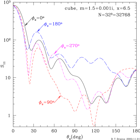
Figure 8: Scattered intensity for incident unpolarized light for a cube with $m=1.5+0.001i$ and $x=2\pi a_{\rm eff}/\lambda=6.5$ (i.e., $d/\lambda=1.6676$, where $d$ is the length of a side). The cube is tilted with respect to the incident radiation, with $\Theta=30^{\circ}$, and rotated by $\beta=15^{\circ}$ around its axis to break reflection symmetry. The Mueller matrix element $S_{11}$ is shown for 4 different scattering planes. The strong forward scattering lobe is evident. It is also seen that the scattered intensity is a strong function of scattering angle $\phi_{s}$ as well as $\theta_{s}$ – at a given value of $\theta_{s}$ (e.g., $\theta_{s}=120^{\circ}$), the scattered intensity can vary by orders of magnitude as $\phi_{s}$ changes by $90^{\circ}$.

An example of scattering by a nonspherical target is shown in Fig. 8, showing the scattering for a tilted cube. Results are shown for four different scattering planes.

DDSCAT automatically carries out numerical integration of various scattering properties, including

• $\langle\cos\theta_{s}\rangle$;

• $\langle\cos^{2}\theta_{s}\rangle$;

• ${\bf g}=\langle\cos\theta_{s}\rangle{\hat{\bf x}}+\langle\sin\theta_{s}\cos\phi_{s}\rangle{\hat{\bf y}}+\langle\sin\theta_{s}\sin\phi_{s}\rangle{\hat{\bf z}}~{}$ (see §15);

• ${\bf Q}_{\Gamma}$, provided option DOTORQ is specified (see §15).

The angular averages are accomplished by evaluating the scattered intensity for selected scattering directions $(\theta_{s},\phi_{s})$, and taking the appropriately weighted sum. Suppose that we have $N_{\theta}$ different values of $\theta_{s}$,

$$\theta=\theta_{j},~{}~{}~{}j=1,...,N_{\theta}~{}~{}~{},$$ (31)

and for each value of $\theta_{j}$, $N_{\phi}(j)$ different values of $\phi_{s}$:

$$\phi_{s}=\phi_{j,k},~{}~{}~{}k=1,...,N_{\phi}(j)~{}~{}~{}.$$ (32)

For a given $j$, the values of $\phi_{j,k}$ are assumed to be uniformly spaced: $\phi_{j,k+1}-\phi_{j,k}=2\pi/N_{\phi}(j)$. The angular average of a quantity $f(\theta_{s},\phi_{s})$ is approximated by

$$\langle f\rangle\equiv\frac{1}{4\pi}\int_{0}^{\pi}\sin\theta_{s}d\theta_{s}\int_{0}^{2\pi}d\phi_{s}f(\theta_{s},\phi_{s})~{}\approx~{}\frac{1}{4\pi}\sum_{j=1}^{N_{\theta}}\sum_{k=1}^{N_{\phi}(j)}f(\theta_{j},\phi_{j,k})\Omega_{j,k}$$ (33)

$$\Omega_{j,k}=\frac{\pi}{N_{\phi}(j)}\left[\cos(\theta_{j-1})-\cos(\theta_{j+1})\right]~{}~{}~{},~{}~{}~{}j=2,...,N_{\theta}-1~{}~{}~{}.$$ (34)

$$\Omega_{1,k}=\frac{2\pi}{N_{\phi}(1)}\left[1-\frac{\cos(\theta_{1})+\cos(\theta_{2})}{2}\right]~{}~{}~{},$$ (35)

$$\Omega_{N_{\theta},k}=\frac{2\pi}{N_{\phi}(N_{\theta})}\left[\frac{\cos(\theta_{N_{\theta}-1})+\cos(\theta_{N_{\theta}})}{2}+1\right]~{}~{}~{}.$$ (36)

For a sufficiently large number of scattering directions

$$N_{\rm sca}\equiv\sum_{j=1}^{N_{\theta}}N_{\phi}(j)$$ (37)

the sum (33) approaches the desired integral, but the calculations can be a significant cpu-time burden, so efficiency is an important consideration.

22.2 Selection of Scattering Angles $\theta_{s},\phi_{s}$

Beginning with DDSCAT 6.1, an improved approach is taken to evaluation of the angular average. Since targets with large values of $x=2\pi a_{\rm eff}/\lambda$ in general have strong forward scattering, it is important to obtain good sampling of the forward scattering direction. To implement a preferential sampling of the forward scattering directions, the scattering directions $(\theta,\phi)$ are chosen so that $\theta$ values correspond to equal intervals in a monotonically increasing function $s(\theta)$. The function $s(\theta)$ is chosen to have a negative second derivative $d^{2}s/d\theta^{2}<0$ so that the density of scattering directions will be higher for small values of $\theta$. DDSCAT 6.1 takes

$$s(\theta)=\theta+\frac{\theta}{\theta+\theta_{0}}~{}~{}~{}.$$ (38)

This provides increased resolution (i.e., increased $ds/d\theta$) for $\theta<\theta_{0}$. We want this for the forward scattering lobe, so we take

$$\theta_{0}=\frac{2\pi}{1+x}~{}~{}.$$ (39)

The $\theta$ values run from $\theta=0$ to $\theta=\pi$, corresponding to uniform increments

$$\Delta s=\frac{1}{N_{\theta}-1}\left(\pi+\frac{\pi}{\pi+\theta_{0}}\right)~{}~{}~{}.$$ (40)

If we now require that

$$\max[\Delta\theta]\approx\frac{\Delta s}{(ds/d\theta)_{\theta=\pi}}=\eta\frac{\pi/2}{3+x}~{}~{}~{},$$ (41)

we determine the number of values of $\theta$:

$$N_{\theta}=1+\frac{2(3+x)}{\eta}\frac{\left[1+1/(\pi+\theta_{0})\right]}{\left[1+\theta_{0}/(\pi+\theta_{0})^{2}\right]}~{}~{}~{}.$$ (42)

Thus for small values of $x$, $\max[\Delta\theta]=30^{\circ}\eta$, and for $x\gg 1$, $\max[\Delta\theta]\rightarrow 90^{\circ}\eta/x$. For a sphere, minima in the scattering pattern are separated by $\sim 180^{\circ}/x$, so $\eta=1$ would be expected to marginally resolve structure in the scattering function. Smaller values of $\eta$ will obviously lead to improved sampling of the scattering function, and more accurate angular averages.

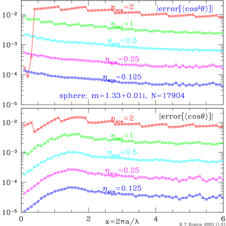
Figure 9: Errors in $\langle\cos\theta\rangle$ and $\langle\cos^{2}\theta\rangle$ calculated for a $N=17904$ dipole pseudosphere with $m=1.33+0.01i$, as functions of $x=2\pi a/\lambda$. Results are shown for different values of the parameter $\eta$.

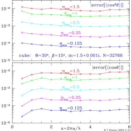
Figure 10: Same as Fig. 9, but for a $N=32768$ dipole cube with $m=1.5+0.001i$.

The scattering angles $\theta_{j}$ used for the angular averaging are then given by

$$\theta_{j}=\frac{(s_{j}-1-\theta_{0})+\left[(1+\theta_{0}-s_{j})^{2}+4\theta_{0}s_{j}\right]^{1/2}}{2}~{}~{}~{},$$ (43)

where

$$s_{j}=\frac{(j-1)\pi}{N_{\theta}-1}\left[1+\frac{1}{\pi+\theta_{0}}\right]~{}~{}~{}j=1,...,N_{\theta}~{}~{}~{}.$$ (44)

For each $\theta_{j}$, we must choose values of $\phi$. For $\theta_{1}=0$ and $\theta_{N_{\theta}}=\pi$ only a single value of $\phi$ is needed (the scattering is independent of $\phi$ in these two directions). For $0<\theta_{j}<\pi$ we use

$$N_{\phi}=\max\left\{3,{\rm nint}\left[4\pi\sin(\theta_{j})/(\theta_{j+1}-\theta_{j-1})\right]\right\}~{}~{}~{},$$ (45)

where ${\rm nint}=$ nearest integer. This provides sampling in $\phi$ consistent with the sampling in $\theta$.

22.3 Accuracy of Angular Averaging as a Function of $\eta$

Figure 9 shows the absolute errors in $\langle\cos\theta\rangle$ and $\langle\cos^{2}\theta\rangle$ calculated for a sphere with refractive index $m=1.33+0.01i$ using the above prescription for choosing scattering angles. The error is shown as a function of scattering parameter $x$. We see that accuracies of order 0.01 are attained with $\eta=1$, and that the above prescription provides an accuracy which is approximately independent of $x$. We recommend using values of $\eta\leq 1$ unless accuracy in the angular averages is not important.

23 Mueller Matrix for Scattering in Selected Directions

23.1 Two Orthogonal Incident Polarizations (IORTH=2)

DDSCAT 6.1 internally computes the scattering properties of the dipole array in terms of a complex scattering matrix $f_{ml}(\theta_{s},\phi_{s})$ (Draine 1988), where index $l=1,2$ denotes the incident polarization state, $m=1,2$ denotes the scattered polarization state, and $\theta_{s}$,$\phi_{s}$ specify the scattering direction. Normally DDSCAT is used with IORTH=2 in ddscat.par, so that the scattering problem will be solved for both incident polarization states ($l=1$ and 2); in this subsection it will be assumed that this is the case.

Incident polarization states $l=1,2$ correspond to polarization states ${\hat{\bf e}}_{01}$, ${\hat{\bf e}}_{02}$; recall that polarization state ${\hat{\bf e}}_{01}$ is user-specified, and ${\hat{\bf e}}_{02}=\hat{\bf x}\times{\hat{\bf e}}_{01}^{*}$. Scattered polarization state $m=1$ corresponds to linear polarization of the scattered wave parallel to the scattering plane (${\hat{\bf e}}_{1}={\hat{\bf e}}_{\parallel s}=\hat{\theta}_{s}$) and $m=2$ corresponds to linear polarization perpendicular to the scattering plane (in the $+\hat{\phi}_{s}$ direction). The scattering matrix $f_{ml}$ was defined (Draine 1988) so that the scattered electric field ${\bf E}_{s}$ is related to the incident electric field ${\bf E}_{i}(0)$ at the origin (where the target is assumed to be located) by

$$\left(\begin{array}[]{c}{\bf E}_{s}\cdot\hat{\theta}_{s}\\ {\bf E}_{s}\cdot\hat{\phi}_{s}\end{array}\right)={\exp(i{\bf k}\cdot{\bf r})\over kr}\left(\begin{array}[]{cc}f_{11}&f_{12}\\ f_{21}&f_{22}\end{array}\right)\left(\begin{array}[]{c}{\bf E}_{i}(0)\cdot{\hat{\bf e}}_{01}\\ {\bf E}_{i}(0)\cdot{\hat{\bf e}}_{02}\end{array}\right)~{}~{}~{}.$$ (46)

The 2$\times$2 complex scattering amplitude matrix (with elements $S_{1}$, $S_{2}$, $S_{3}$, and $S_{4}$) is defined so that (see Bohren & Huffman 1983)

$$\left(\begin{array}[]{c}{\bf E}_{s}\cdot\hat{\theta}_{s}\\ -{\bf E}_{s}\cdot\hat{\phi}_{s}\end{array}\right)={\exp(i{\bf k}\cdot{\bf r})\over-ikr}\left(\begin{array}[]{cc}S_{2}&S_{3}\\ S_{4}&S_{1}\end{array}\right)\left(\begin{array}[]{c}{\bf E}_{i}(0)\cdot{\hat{\bf e}}_{i\parallel}\\ {\bf E}_{i}(0)\cdot{\hat{\bf e}}_{i\perp}\end{array}\right)~{}~{}~{},$$ (47)

where ${\hat{\bf e}}_{i\parallel}$, ${\hat{\bf e}}_{i\perp}$ are (real) unit vectors for incident polarization parallel and perpendicular to the scattering plane (with the customary definition of ${\hat{\bf e}}_{i\perp}={\hat{\bf e}}_{i\parallel}\times{\hat{\bf x}}$).

From (46,47) we may write

$$\left(\begin{array}[]{cc}S_{2}&S_{3}\\ S_{4}&S_{1}\end{array}\right)\left(\begin{array}[]{c}{\bf E}_{i}(0)\cdot{\hat{\bf e}}_{i\parallel}\\ {\bf E}_{i}(0)\cdot{\hat{\bf e}}_{i\perp}\end{array}\right)=-i\left(\begin{array}[]{cc}f_{11}&f_{12}\\ -f_{21}&-f_{22}\end{array}\right)\left(\begin{array}[]{c}{\bf E}_{i}(0)\cdot{\hat{\bf e}}_{01}^{*}\\ {\bf E}_{i}(0)\cdot{\hat{\bf e}}_{02}^{*}\end{array}\right)~{}~{}~{}.$$ (48)

Let

$$a \equiv {\hat{\bf e}}_{01}^{*}\cdot{\hat{\bf y}}~{}~{}~{},$$ (49)

$$b \equiv {\hat{\bf e}}_{01}^{*}\cdot{\hat{\bf z}}~{}~{}~{},$$ (50)

$$c \equiv {\hat{\bf e}}_{02}^{*}\cdot{\hat{\bf y}}~{}~{}~{},$$ (51)

$$d \equiv {\hat{\bf e}}_{02}^{*}\cdot{\hat{\bf z}}~{}~{}~{}.$$ (52)

Note that since ${\hat{\bf e}}_{01},{\hat{\bf e}}_{02}$ could be complex (i.e., elliptical polarization), the quantities $a,b,c,d$ are complex. Then

$$\left(\begin{array}[]{c}{\hat{\bf e}}_{01}^{*}\\ {\hat{\bf e}}_{02}^{*}\end{array}\right)=\left(\begin{array}[]{cc}a&b\\ c&d\end{array}\right)\left(\begin{array}[]{c}\hat{\bf y}\\ \hat{\bf z}\end{array}\right)$$ (53)

and eq. (48) can be written

$$\left(\begin{array}[]{cc}S_{2}&S_{3}\\ S_{4}&S_{1}\end{array}\right)\left(\begin{array}[]{c}{\bf E}_{i}(0)\cdot{\hat{\bf e}}_{i\parallel}\\ {\bf E}_{i}(0)\cdot{\hat{\bf e}}_{i\perp}\end{array}\right)=i\left(\begin{array}[]{cc}-f_{11}&-f_{12}\\ f_{21}&f_{22}\end{array}\right)\left(\begin{array}[]{cc}a&b\\ c&d\end{array}\right)\left(\begin{array}[]{c}{\bf E}_{i}(0)\cdot\hat{\bf y}\\ {\bf E}_{i}(0)\cdot\hat{\bf z}\end{array}\right)~{}~{}~{}.$$ (54)

The incident polarization states ${\hat{\bf e}}_{i\parallel}$ and ${\hat{\bf e}}_{i\perp}$ are related to $\hat{\bf y}$, $\hat{\bf z}$ by

$$\left(\begin{array}[]{c}\hat{\bf y}\\ \hat{\bf z}\end{array}\right)=\left(\begin{array}[]{cc}\cos\phi_{s}&\sin\phi_{s}\\ \sin\phi_{s}&-\cos\phi_{s}\end{array}\right)\left(\begin{array}[]{c}{\hat{\bf e}}_{i\parallel}\\ {\hat{\bf e}}_{i\perp}\end{array}\right);$$ (55)

substituting (55) into (54) we obtain

$$\left(\!\begin{array}[]{cc}S_{2}&S_{3}\\ S_{4}&S_{1}\end{array}\!\right)\left(\!\begin{array}[]{c}{\bf E}_{i}(0)\cdot{\hat{\bf e}}_{i\parallel}\\ {\bf E}_{i}(0)\cdot{\hat{\bf e}}_{i\perp}\end{array}\!\right)=i\left(\!\begin{array}[]{cc}-f_{11}&-f_{12}\\ f_{21}&f_{22}\end{array}\!\right)\left(\!\begin{array}[]{cc}a&b\\ c&d\end{array}\!\right)\left(\!\begin{array}[]{cc}\cos\phi_{s}&\sin\phi_{s}\\ \sin\phi_{s}&-\cos\phi_{s}\end{array}\!\right)\left(\!\begin{array}[]{c}{\bf E}_{i}(0)\cdot{\hat{\bf e}}_{i\parallel}\\ {\bf E}_{i}(0)\cdot{\hat{\bf e}}_{i\perp}\end{array}\!\right)$$ (56)

Eq. (56) must be true for all ${\bf E}_{i}(0)$, so we obtain an expression for the complex scattering amplitude matrix in terms of the $f_{ml}$:

$$\left(\begin{array}[]{cc}S_{2}&S_{3}\\ S_{4}&S_{1}\end{array}\right)=i\left(\begin{array}[]{cc}-f_{11}&-f_{12}\\ f_{21}&f_{22}\end{array}\right)\left(\begin{array}[]{cc}a&b\\ c&d\end{array}\right)\left(\begin{array}[]{cc}\cos\phi_{s}&\sin\phi_{s}\\ \sin\phi_{s}&-\cos\phi_{s}\end{array}\right)~{}~{}~{}.$$ (57)

This provides the 4 equations used in subroutine GETMUELLER to compute the scattering amplitude matrix elements:

$$S_{1} = -i\left[f_{21}(b\cos\phi_{s}-a\sin\phi_{s})+f_{22}(d\cos\phi_{s}-c\sin\phi_{s})\right]~{}~{}~{},$$ (58)

$$S_{2} = -i\left[f_{11}(a\cos\phi_{s}+b\sin\phi_{s})+f_{12}(c\cos\phi_{s}+d\sin\phi_{s})\right]~{}~{}~{},$$ (59)

$$S_{3} = i\left[f_{11}(b\cos\phi_{s}-a\sin\phi_{s})+f_{12}(d\cos\phi_{s}-c\sin\phi_{s})\right]~{}~{}~{},$$ (60)

$$S_{4} = i\left[f_{21}(a\cos\phi_{s}+b\sin\phi_{s})+f_{22}(c\cos\phi_{s}+d\sin\phi_{s})\right]~{}~{}~{}.$$ (61)

23.2 Stokes Parameters

It is both convenient and customary to characterize both incident and scattered radiation by 4 “Stokes parameters” – the elements of the “Stokes vector”. There are different conventions in the literature; we adhere to the definitions of the Stokes vector ($I$,$Q$,$U$,$V$) adopted in the excellent treatise by Bohren & Huffman (1983), to which the reader is referred for further detail. Here are some examples of Stokes vectors $(I,Q,U,V)=(1,Q/I,U/I,V/I)I$:

• $(1,0,0,0)I$ : unpolarized light (with intensity $I$);

• $(1,1,0,0)I$ : 100% linearly polarized with ${\bf E}$ parallel to the scattering plane;

• $(1,-1,0,0)I$ : 100% linearly polarized with ${\bf E}$ perpendicular to the scattering plane;

• $(1,0,1,0)I$ : 100% linearly polarized with ${\bf E}$ at +45^∘ relative to the scattering plane;

• $(1,0,-1,0)I$ : 100% linearly polarized with ${\bf E}$ at -45^∘ relative to the scattering plane;

• $(1,0,0,1)I$ : 100% right circular polarization (i.e., negative helicity);

• $(1,0,0,-1)I$ : 100% left circular polarization (i.e., positive helicity).

23.3 Relation Between Stokes Parameters of Incident and Scattered Radiation: The Mueller Matrix

It is convenient to describe the scattering properties in terms of the $4\times 4$ Mueller matrix relating the Stokes parameters $(I_{i},Q_{i},U_{i},V_{i})$ and $(I_{s},Q_{s},U_{s},V_{s})$ of the incident and scattered radiation:

$$\left(\begin{array}[]{c}I_{s}\\ Q_{s}\\ U_{s}\\ V_{s}\end{array}\right)={1\over k^{2}r^{2}}\left(\begin{array}[]{cccc}S_{11}&S_{12}&S_{13}&S_{14}\\ S_{21}&S_{22}&S_{23}&S_{24}\\ S_{31}&S_{32}&S_{33}&S_{34}\\ S_{41}&S_{42}&S_{43}&S_{44}\end{array}\right)\left(\begin{array}[]{c}I_{i}\\ Q_{i}\\ U_{i}\\ V_{i}\end{array}\right)~{}~{}~{}.$$ (62)

Once the amplitude scattering matrix elements are obtained, the Mueller matrix elements can be computed (Bohren & Huffman 1983):

$$S_{11} = \left(|S_{1}|^{2}+|S_{2}|^{2}+|S_{3}|^{2}+|S_{4}|^{2}\right)/2~{}~{}~{},$$

$$S_{12} = \left(|S_{2}|^{2}-|S_{1}|^{2}+|S_{4}|^{2}-|S_{3}|^{2}\right)/2~{}~{}~{},$$

$$S_{13} = {\rm Re}\left(S_{2}S_{3}^{*}+S_{1}S_{4}^{*}\right)~{}~{}~{},$$

$$S_{14} = {\rm Im}\left(S_{2}S_{3}^{*}-S_{1}S_{4}^{*}\right)~{}~{}~{},$$

$$S_{21} = \left(|S_{2}|^{2}-|S_{1}|^{2}+|S_{3}|^{2}-|S_{4}|^{2}\right)/2~{}~{}~{},$$

$$S_{22} = \left(|S_{1}|^{2}+|S_{2}|^{2}-|S_{3}|^{2}-|S_{4}|^{2}\right)/2~{}~{}~{},$$

$$S_{23} = {\rm Re}\left(S_{2}S_{3}^{*}-S_{1}S_{4}^{*}\right)~{}~{}~{},$$

$$S_{24} = {\rm Im}\left(S_{2}S_{3}^{*}+S_{1}S_{4}^{*}\right)~{}~{}~{},$$

$$S_{31} = {\rm Re}\left(S_{2}S_{4}^{*}+S_{1}S_{3}^{*}\right)~{}~{}~{},$$

$$S_{32} = {\rm Re}\left(S_{2}S_{4}^{*}-S_{1}S_{3}^{*}\right)~{}~{}~{},$$

$$S_{33} = {\rm Re}\left(S_{1}S_{2}^{*}+S_{3}S_{4}^{*}\right)~{}~{}~{},$$

$$S_{34} = {\rm Im}\left(S_{2}S_{1}^{*}+S_{4}S_{3}^{*}\right)~{}~{}~{},$$

$$S_{41} = {\rm Im}\left(S_{4}S_{2}^{*}+S_{1}S_{3}^{*}\right)~{}~{}~{},$$

$$S_{42} = {\rm Im}\left(S_{4}S_{2}^{*}-S_{1}S_{3}^{*}\right)~{}~{}~{},$$

$$S_{43} = {\rm Im}\left(S_{1}S_{2}^{*}-S_{3}S_{4}^{*}\right)~{}~{}~{},$$

$$S_{44} = {\rm Re}\left(S_{1}S_{2}^{*}-S_{3}S_{4}^{*}\right)~{}~{}~{}.$$ (63)

These matrix elements are computed in DDSCAT and passed to subroutine WRITESCA which handles output of scattering properties. Although the Muller matrix has 16 elements, only 9 are independent.

The user can select up to 9 distinct Muller matrix elements to be printed out in the output files wxxryykzzz.sca and wxxryyori.avg; this choice is made by providing a list of indices in ddscat.par (see Appendix A).

If the user does not provide a list of elements, WRITESCA will provide a “default” set of 6 selected elements: $S_{11}$, $S_{21}$, $S_{31}$, $S_{41}$ (these 4 elements describe the intensity and polarization state for scattering of unpolarized incident radiation), $S_{12}$, and $S_{13}$.

In addition, WRITESCA writes out the linear polarization $P$ of the scattered light for incident unpolarized light (Bohren & Huffman 1983, p. 382)

$$P=-{S_{12}\over S_{11}}~{}~{}~{}.$$ (64)

23.4 Polarization Properties of the Scattered Radiation

The scattered radiation is fully characterized by its Stokes vector $(I_{s},Q_{s},U_{s},V_{s})$. As discussed in Bohren & Huffman (eq. 2.87), one can determine the linear polarization of the Stokes vector by operating on it by the Mueller matrix of an ideal linear polarizer:

$${\bf S}_{\rm pol}=\frac{1}{2}\left(\begin{array}[]{cccc}1&\cos 2\xi&\sin 2\xi&0\\ \cos 2\xi&\cos^{2}2\xi&\cos 2\xi\sin 2\xi&0\\ \sin 2\xi&\sin 2\xi\cos 2\xi&\sin^{2}2\xi&0\\ 0&0&0&0\\ \end{array}\right)$$ (65)

where $\xi$ is the angle between the unit vector $\hat{\theta}_{s}$ parallel to the scattering plane (“SP”) and the “transmission” axis of the linear polarizer. Therefore the intensity of light polarized parallel to the scattering plane is obtained by taking $\xi=0$ and operating on $(I_{s},Q_{s},U_{s},V_{s})$ to obtain

$$I({\bf E}_{s}\parallel{\rm SP}) = \frac{1}{2}(I_{s}+Q_{s})$$ (66)

$$= \frac{1}{2k^{2}r^{2}}\left[(S_{11}+S_{21})I_{i}+(S_{12}+S_{22})Q_{i}+(S_{13}+S_{23})U_{i}+(S_{14}+S_{24})V_{i}\right]~{}.~{}~{}~{}~{}~{}$$ (67)

Similarly, the intensity of light polarized perpendicular to the scattering plane is obtained by taking $\xi=\pi/2$:

$$I({\bf E}_{s}\perp{\rm SP}) = \frac{1}{2}(I_{s}-Q_{s})$$ (68)

$$= \frac{1}{2k^{2}r^{2}}\left[(S_{11}-S_{21})I_{i}+(S_{12}-S_{22})Q_{i}+(S_{13}-S_{23})U_{i}+(S_{14}-S_{24})V_{i}\right]~{}.~{}~{}~{}~{}~{}$$ (69)

23.5 Relation Between Mueller Matrix and Scattering Cross Sections

Differential scattering cross sections can be obtained directly from the Mueller matrix elements by noting that

$$I_{s}=\frac{1}{r^{2}}\left(\frac{dC_{\rm sca}}{d\Omega}\right)_{s,i}I_{i}~{}~{}~{}.$$ (70)

Let SP be the “scattering plane”: the plane containing the incident and scattered directions of propagation. Here we consider some special cases:

• Incident light unpolarized: Stokes vector $s_{i}=I(1,0,0,0)$:

  • cross section for scattering with polarization ${\bf E}_{s}\parallel$ SP:

    $$\frac{dC_{\rm sca}}{d\Omega}=\frac{1}{2k^{2}}\left(|S_{2}|^{2}+|S_{3}|^{2}\right)=\frac{1}{2k^{2}}\left(S_{11}+S_{21}\right)$$ (71)

  • cross section for scattering with polarization ${\bf E}_{s}\perp$ SP:

    $$\frac{dC_{\rm sca}}{d\Omega}=\frac{1}{2k^{2}}\left(|S_{1}|^{2}+|S_{4}|^{2}\right)=\frac{1}{2k^{2}}\left(S_{11}-S_{21}\right)$$ (72)

  • total intensity of scattered light:

    $$\frac{dC_{\rm sca}}{d\Omega}=\frac{1}{2k^{2}}\left(|S_{1}|^{2}+|S_{2}|^{2}+|S_{3}|^{2}+|S_{4}|^{2}\right)=\frac{1}{k^{2}}S_{11}$$ (73)

• Incident light polarized with ${\bf E}_{i}\parallel$ SP: Stokes vector $s_{i}=I(1,1,0,0)$:

  • cross section for scattering with polarization ${\bf E}_{s}\parallel$ to SP:

    $$\frac{dC_{\rm sca}}{d\Omega}=\frac{1}{k^{2}}|S_{2}|^{2}=\frac{1}{2k^{2}}\left(S_{11}+S_{12}+S_{21}+S_{22}\right)$$ (74)

  • cross section for scattering with polarization ${\bf E}_{s}\perp$ to SP:

    $$\frac{dC_{\rm sca}}{d\Omega}=\frac{1}{k^{2}}|S_{4}|^{2}=\frac{1}{2k^{2}}\left(S_{11}+S_{12}-S_{21}-S_{22}\right)$$ (75)

  • total scattering cross section:

    $$\frac{dC_{\rm sca}}{d\Omega}=\frac{1}{k^{2}}\left(|S_{2}|^{2}+|S_{4}|^{2}\right)=\frac{1}{k^{2}}\left(S_{11}+S_{12}\right)$$ (76)

• Incident light polarized with ${\bf E}_{i}\perp$ SP: Stokes vector $s_{i}=I(1,-1,0,0)$:

  • cross section for scattering with polarization ${\bf E}_{s}\parallel$ to SP:

    $$\frac{dC_{\rm sca}}{d\Omega}=\frac{1}{k^{2}}|S_{3}|^{2}=\frac{1}{2k^{2}}\left(S_{11}-S_{12}+S_{21}-S_{22}\right)$$ (77)

  • cross section for scattering with polarization ${\bf E}_{s}\perp$ SP:

    $$\frac{dC_{\rm sca}}{d\Omega}=\frac{1}{k^{2}}|S_{1}|^{2}=\frac{1}{2k^{2}}\left(S_{11}-S_{12}-S_{21}+S_{22}\right)$$ (78)

  • total scattering cross section:

    $$\frac{dC_{\rm sca}}{d\Omega}=\frac{1}{k^{2}}\left(|S_{1}|^{2}+|S_{3}|^{2}\right)=\frac{1}{k^{2}}\left(S_{11}-S_{12}\right)$$ (79)

• Incident light linearly polarized at angle $\gamma$ to SP: Stokes vector $s_{i}=I(1,\cos 2\gamma,\sin 2\gamma,0)$:

  • cross section for scattering with polarization ${\bf E}_{s}\parallel$ to SP:

    $$\frac{dC_{\rm sca}}{d\Omega}=\frac{1}{2k^{2}}\left[(S_{11}+S_{21})+(S_{12}+S_{22})\cos 2\gamma+(S_{13}+S_{23})\sin 2\gamma\right]$$ (80)

  • cross section for scattering with polarization ${\bf E}_{s}\perp$ SP:

    $$\frac{dC_{\rm sca}}{d\Omega}=\frac{1}{2k^{2}}\left[(S_{11}-S_{21})+(S_{12}-S_{22})\cos 2\gamma+(S_{13}-S_{23})\sin 2\gamma\right]$$ (81)

  • total scattering cross section:

    $$\frac{dC_{\rm sca}}{d\Omega}=\frac{1}{k^{2}}\left[S_{11}+S_{12}\cos 2\gamma+S_{13}\sin 2\gamma\right]$$ (82)

23.6 One Incident Polarization State Only (IORTH=1)

In some cases it may be desirable to limit the calculations to a single incident polarization state – for example, when each solution is very time-consuming, and the target is known to have some symmetry so that solving for a single incident polarization state may be sufficient for the required purpose. In this case, set IORTH=1 in ddscat.par.

When IORTH=1, only $f_{11}$ and $f_{21}$ are available; hence, DDSCAT cannot automatically generate the Mueller matrix elements. In this case, the output routine WRITESCA writes out the quantities $|f_{11}|^{2}$, $|f_{21}|^{2}$, ${\rm Re}(f_{11}f_{21}^{*})$, and ${\rm Im}(f_{11}f_{21}^{*})$ for each of the scattering directions.

The differential scattering cross section for scattering with polarization ${\bf E}_{s}\parallel$ and $\perp$ to the scattering plane are

$$\left(\frac{dC_{\rm sca}}{d\Omega}\right)_{s,\parallel} = \frac{1}{k^{2}}|f_{11}|^{2}$$ (83)

$$\left(\frac{dC_{\rm sca}}{d\Omega}\right)_{s,\perp} = \frac{1}{k^{2}}|f_{21}|^{2}$$ (84)

Note, however, that if IPHI is greater than 1, DDSCAT will automatically set IORTH=2 even if ddscat.par specified IORTH=1: this is because when more than one value of the target orientation angle $\Phi$ is required, there is no additional “cost” to solve the scattering problem for the second incident polarization state, since when solutions are available for two orthogonal states for some particular target orientation, the solution may be obtained for another target orientation differing only in the value of $\Phi$ by appropriate linear combinations of these solutions. Hence we may as well solve the “complete” scattering problem so that we can compute the complete Mueller matrix.

24 Using MPI (Message Passing Interface)

Many (probably most) users of DDSCAT will wish to calculate scattering and absorption by a given target for more than one orientation relative to the incident radiation (e.g., when calculating orientational averages). DDSCAT can automatically carry out the calculations over different target orientations. Normally, these calculations will be carried out sequentially. However, on a multiprocessor system [either a symmetric multiprocessor (SMP) system, or a cluster of networked computers] with MPI (Message Passing Interface) software installed, DDSCAT 6.1 allows the user to carry out parallel calculations of scattering by different target orientations, with the results gathered together and with orientational averages calculated just as they are when sequential calculations are carried out. Note that the MPI-capable executable can also be used for ordinary serial calculations using a single cpu.

More than one implementation of MPI exists. MPI support within DDSCAT 6.1 is compliant with MPI-1.2 and MPI-2 standards, and should be usable under any implementation of MPI that is compatible with those standards.

At Princeton University Department of Astrophysical Sciences we are using MPICH, a publicly-available implementation of MPI.

24.1 Source Code for the MPI-compatible version of DDSCAT

In order to use DDSCAT with MPI, the user must first make sure that the correct version of the code is being used. To prepare the MPI-capable version:

1. In DDSCAT.f :

   • Make sure the line
                 INCLUDE ’mpif.h’
     is not commented out.

   • Make sure the line
     C         INTEGER MPI_COMM_WORLD
     is commented out.

2. In mpisubs.f, SUBROUTINE COLSUM :

   • Make sure the line
                 INCLUDE ’mpif.h’
     is not commented out.

   • Make sure the line
     C         INTEGER MPI_COMM_WORLD,MPI_SUM,MPI_REAL,MPI_COMPLEX
     is commented out.

3. In mpisubs.f, SUBROUTINE SHARE1 :

   • Make sure the line
                 INCLUDE ’mpif.h’
     is not commented out.

   • Make sure the lines
     C         INTEGER MPI_CHARACTER,MPI_COMM_WORLD,MPI_INTEGER,
     C        &      MPI_INTEGER2,MPI_REAL,MPI_COMPLEX

     are commented out.

4. In mpisubs.f, SUBROUTINE SHARE2 :

   • Make sure the line
                 INCLUDE ’mpif.h’
     is not commented out.

   • Make sure the line
     C         INTEGER MPI_COMM_WORLD,MPI_REAL,MPI_COMPLEX

     is commented out.

24.2 Compiling and Linking the MPI-compatible version of DDSCAT

In the Makefile, enable the following definitions:
         MPIsrc         = mpi_subs.f
         MPIobj         = mpi_subs.o

At Princeton University Dept. of Astrophysical Sciences we are currently using mpich-1.2.4. mpich provides a “compiler wrapper” mpif77 that is supposed to automatically set the variables MPICH_F77 and MPICH_F77LINKER to values appropriate for use of the pgf77 compiler from PGI which is installed on our beowulf cluster. Other compilers, e.g., the Intel f77 compiler, can also be employed.

24.3 Code Execution Under MPI

Local installations of MPI will vary – you should consult with someone familiar with way MPI is installed and used on your system.

At Princeton University Dept. of Astrophysical Sciences we use PBS (Portable Batch System) to schedule jobs. MPI jobs are submitted using PBS by first creating a shell script such as the following example file pbs.submit:

     #!/bin/bash
     #PBS -l nodes=2:ppn=1
     #PBS -l mem=1200MB,pmem=300MB
     #PBS -m bea
     #PBS -j oe
     cd $PBS_O_WORKDIR
     /usr/local/bin/mpiexec ddscat

The lines beginning with #PBS -l specify the required resources:
#PBS -l nodes=2:ppn=1 specifies that 2 nodes are to be used, with 1 processor per node.
#PBS -l mem=1200MB,pmem=300MB specifies that the total memory required (mem) is 1200MB, and the maximum physical memory used by any single process (pmem) is 300MB. The actual definition of mem is not clear, but in practice it seems that it should be set equal to 2$\times$(nodes)$\times$(ppn)$\times$(pmem) .
#PBS -m bea specifies that PBS should send email when the job begins (b), and when it ends (e) or aborts (a).
#PBS -j oe specifies that the output from stdout and stderr will be merged, intermixed, as stdout.

This example assumes that the executable dscat is located in the same directory where the code is to execute and write its output. If ddscat is located in another directory, simply give the full pathname. to it. The qsub command is used to submit the PBS job:

% qsub pbs.submit

As the calculation proceeds, the usual output files will be written to this directory: for each wavelength, target size, and target orientation, there will be a file waarbbkccc.sca, where aa=00, 01, 02, … specifies the wavelength, bb=00, 01, 02, … specifies the target size, and cc=000, 001, 002, … specifies the orientation. For each wavelength and target size there will also be a file waarbbori.avg with orientationally-averaged quantities. Finally, there will also be tables qtable, and qtable2 with orientationally-averaged cross sections for each wavelength and target size.

In addition, each processor employed will write to its own log file ddscat.log_nnn, where nnn=000, 001, 002, …. These files contain information concerning cpu time consumed by different parts of the calculation, convergence to the specified error tolerance, etc. If you are uncertain about how the calculation proceeded, examination of these log files is recommended.

25 Graphics and Postprocessing

25.1 IDL

At present, we do not offer a comprehensive package for DDSCAT data postprocessing and graphical display in IDL. However, there are several developments worth mentioning: First, we offer several output capabilities from within DDSCAT: ASCII (see §10.1), FORTRAN unformatted binary (see §10.2), and netCDF portable binary (see §10.3). Second, we offer several skeleton IDL utilities:

• bhmie.pro is our translation to IDL of the popular Bohren-Huffman code which calculates efficiencies for spherical particles using Mie theory.

• readbin.pro reads the FORTRAN unformatted binary file written by routine writebin.f. The variables are stored in a common block.

• readnet.pro reads NetCDF portable binary file and should be the method of choice for IDL users. It offers random data access.

• mie.pro is an example of an interface to binary files and the Bohren-Huffman code. It plots a comparison of DDSCAT results with scattering by equivalent radius spheres.

At present the IDL code is experimental.

26 Miscellanea

Additional source code, refractive index files, etc., contributed by users will be located in the directory DDA/misc. These routines and files should be considered to be not supported by Draine and Flatau – caveat receptor! These routines and files should be accompanied by enough information (e.g., comments in source code) to explain their use.

27 Finale

This User Guide is somewhat inelegant, but we hope that it will prove useful. The structure of the ddscat.par file is intended to be simple and suggestive so that, after reading the above notes once, the user may not have to refer to them again.

The file rel_notes in DDA/doc lists known bugs in DDSCAT 6.1 . Up-to-date release notes will be available at the DDSCAT web site,
      http://www.astro.princeton.edu/$\sim$draine/DDSCAT.html

Users are encouraged to provide B. T. Draine (draine@astro.princeton.edu) with their email address; bug reports, and any new releases of DDSCAT, will be made known to those who do!

P. J. Flatau maintains the WWW page “SCATTERLIB - Light Scattering Codes Library” with URL http://atol.ucsd.edu/$\sim$pflatau. The SCATTERLIB Internet site is a library of light scattering codes. Emphasis is on providing source codes (mostly FORTRAN). However, other information related to scattering on spherical and non-spherical particles is collected: an extensive list of references to light scattering methods, refractive index, etc. This URL page contains section on the discrete dipole approximation.

Concrete suggestions for improving DDSCAT (and this User Guide) are welcomed. If you wish to cite this User Guide, we suggest the following citation:

Draine, B.T., & Flatau, P.J. 2004, “User Guide for the Discrete Dipole Approximation Code DDSCAT (Version 6.1)”, http://arxiv.org/abs/astro-ph/0409262

Finally, the authors have one special request: We would very much appreciate preprints and (especially!) reprints of any papers which make use of DDSCAT!

28 Acknowledgments

• The routine ESELF making use of the FFT was originally written by Jeremy Goodman, Princeton University Observatory.

• The FFT routine FOURX, used in the comparison of different FFT routines, is based on a FFT routine written by Norman Brenner (Brenner 1969).

• The routine REFICE was written by Steven B. Warren, based on Warren (1984).

• The routine REFWAT was written by Eric A. Smith.

• The GPFAPACK package was written by Clive Temperton (1992), and generously made available by him for use with DDSCAT.

• LAPACK

• We make use of routines from the LAPACK package (Anderson et al. 1995), the result of work by Jack Dongarra and others at the Univ. of Tennessee, Univ. of California Berkeley, NAG Ltd., Courant Institute, Argonne National Lab, and Rice University.

• The FFTW package, to which we link, was written by Matteo Frigo and Steven G. Johnson (fftw@fftw.org).

• Much of the work involved in modifying DDSCAT to use MPI was done by Matthew Collinge, Princeton University.

We are deeply indebted to all of these authors for making their code available.

We wish also to acknowledge bug reports and suggestions from DDSCAT users, including Henrietta Lemke, Fernando Moreno Danvila, Timo Nousianen, and Mike Wolff.

Development of DDSCAT was supported in part by National Science Foundation grants AST-8341412, AST-8612013, AST-9017082, AST-9319283, AST-9616429, AST-9988126, AST-0406883 to BTD, in part by support from the Office of Naval Research Young Investigator Program to PJF, in part by DuPont Corporate Educational Assistance to PJF, and in part by the United Kingdom Defence Research Agency.

Appendix A Understanding and Modifying ddscat.par

In order to use DDSCAT to perform the specific calculations of interest to you, it will be necessary to modify the ddscat.par file. Here we list the sample ddscat.par file, followed by a discussion of how to modify this file as needed. Note that all numerical input data in DDSCAT is read with free-format READ(IDEV,*)... statements. Therefore you do not need to worry about the precise format in which integer or floating point numbers are entered on a line. The crucial thing is that lines in ddscat.par containing numerical data have the correct number of data entries, with any informational comments appearing after the numerical data on a given line.

’ =================== Parameter file ===================’
’**** PRELIMINARIES ****’
’NOTORQ’= CMTORQ*6 (DOTORQ, NOTORQ) -- either do or skip torque calculations
’PBCGST’= CMDSOL*6 (PBCGST, PETRKP) -- select solution method
’GPFAFT’= CMETHD*6 (GPFAFT, FFTWJ, CONVEX)
’LATTDR’= CALPHA*6 (LATTDR, SCLDR)
’NOTBIN’= CBINFLAG (ALLBIN, ORIBIN, NOTBIN)
’NOTCDF’= CNETFLAG (ALLCDF, ORICDF, NOTCDF)
’RCTNGL’= CSHAPE*6 (FRMFIL,ELLIPS,CYLNDR,RCTNGL,HEXGON,TETRAH,UNICYL,...)
32 24 16 = shape parameters PAR1, PAR2, PAR3
1         = NCOMP = number of dielectric materials
’TABLES’= CDIEL*6 (TABLES,H2OICE,H2OLIQ; if TABLES, then filenames follow...)
’diel.tab’ = name of file containing dielectric function
’**** CONJUGATE GRADIENT DEFINITIONS ****’
0       = INIT (TO BEGIN WITH |X0> = 0)
1.00e-5 = TOL = MAX ALLOWED (NORM OF |G>=AC|E>-ACA|X>)/(NORM OF AC|E>)
’**** Angular resolution for calculation of <cos>, etc. ****’
0.5Ψ= ETASCA (number of angles is proportional to [(3+x)/ETASCA]^2 )
’**** Wavelengths (micron) ****’
6.283185 6.283185 1 ’INV’ = wavelengths (first,last,how many,how=LIN,INV,LOG)
’**** Effective Radii (micron) **** ’
2 2 1 ’LIN’ = eff. radii (first, last, how many, how=LIN,INV,LOG)
’**** Define Incident Polarizations ****’
(0,0) (1.,0.) (0.,0.) = Polarization state e01 (k along x axis)
2 = IORTH  (=1 to do only pol. state e01; =2 to also do orth. pol. state)
1 = IWRKSC (=0 to suppress, =1 to write ".sca" file for each target orient.
’**** Prescribe Target Rotations ****’
0.   0.   1  = BETAMI, BETAMX, NBETA (beta=rotation around a1)
0.  90.   3  = THETMI, THETMX, NTHETA (theta=angle between a1 and k)
0.   0.   1  = PHIMIN, PHIMAX, NPHI (phi=rotation angle of a1 around k)
’**** Specify first IWAV, IRAD, IORI (normally 0 0 0) ****’
0   0   0    = first IWAV, first IRAD, first IORI (0 0 0 to begin fresh)
’**** Select Elements of S_ij Matrix to Print ****’
6Ψ= NSMELTS = number of elements of S_ij to print (not more than 9)
11 12 21 22 31 41Ψ= indices ij of elements to print
’**** Specify Scattered Directions ****’
0.  0. 180. 10 = phi, thetan_min, thetan_max, dtheta (in degrees) for plane A
90. 0. 180. 10 = phi, ... for plane B

Lines	Comments
1-2	comment lines – no need to change.
3	NOTORQ if torque calculation is not required;
	DOTORQ if torque calculation is required.
4	PBCGST is recommended; other option is PETRKP (see §14).
5	GPFAFT is supplied as default, but FFTW21 is recommended if DDSCAT has been compiled with
	FFTW support (see §§6.2.5, 13); only other option is CONVEX (valid only on a Convex computer).
6	LATTDR (Draine & Goodman [2000] Lattice Dispersion Relation is only option now supported)
	(see §11).
7	ALLBIN for full unformatted binary dump (§10.2);
	ORIBIN for unformatted binary dump of orientational averages only;
	NOTBIN for no unformatted binary output.
8	ALLCDF for output in netCDF format (must have netCDF option enabled; cf. §10.3);
	ORICDF for orientational averages in netCDF format (must have netCDF option enabled).
	NOTCDF for no output in netCDF format;
9	specify choice of target shape (see §19 for description of options RCTNGL, ELLIPS, TETRAH, …)
10	shape parameters SHPAR1, SHPAR2, SHPAR3, … (see §19).
11	number of different dielectric constant tables (§12).
12	TABLES – dielectric function to be provided via input table.
13	name(s) of dielectric constant table(s) (one per line).
14	comment line – no need to change.
15	0 is recommended value of parameter INIT.
16	TOL = error tolerance $h$: maximum allowed value of $|A^{\dagger}E-A^{\dagger}AP|/|A^{\dagger}E|$ [see eq.(18)].
17	comment line – no need to change.
18	ETASCA – parameter $\eta$ controlling angular averages (§22).
19	comment line – no need to change.
20	$\lambda$ – first, last, how many, how chosen.
21	comment line – no need to change.
22	$a_{\rm eff}$ – first, last, how many, how chosen.
23	comment line – no need to change.
24	specify x,y,z components of (complex) incident polarization ${\hat{\bf e}}_{01}$ (§21)
25	IORTH = 1 to do one polarization state only;
	2 to do second (orthogonal) incident polarization as well.
26	IWRKSC = 0 to suppress writing of “.sca” files;
	2 to enable writing of “.sca” files.
27	comment line – no need to change.
28	$\beta$ (see §17) – first, last, how many .
30	$\Theta$ – first, last, how many.
31	$\Phi$ – first, last, how many.
32	comment line – no need to change.
33	IWAV0 IRAD0 IORI0 – specify starting values of integers IWAV IRAD IORI (normally 0 0 0).
34	comment line – no need to change.
35	$N_{S}$ = number of scattering matrix elements (must be $\leq 9$)
36	indices $ij$ of $N_{S}$ elements of the scattering matrix $S_{ij}$
37	comment line – no need to change.
38	$\phi_{s}$ for first scattering plane, $\theta_{s,min}$, $\theta_{s,max}$, how many $\theta_{s}$ values;
39,…	$\phi_{s}$ for 2nd,… scattering plane, …

Appendix B wxxxryyori.avg Files

The file w000r00ori.avg contains the results for the first wavelength (w000) and first target radius (r00) averaged over orientations (ori.avg). The w000r00ori.avg file generated by the sample calculation should look like the following:

 DDSCAT --- DDSCAT 6.1 [05.10.18]
 TARGET --- Rectangular prism; NX,NY,NZ=  32  24  16
 GPFAFT --- method of solution
 LATTDR --- prescription for polarizabilies
 RCTNGL --- shape
  12288 = NAT0 = number of dipoles
  AEFF=   2.00000 = effective radius (physical units)
  WAVE=   6.28319 = wavelength (physical units)
K*AEFF=   2.00000 = 2*pi*aeff/lambda
n= ( 1.3300 ,  0.0100),  eps.= (  1.7688 ,  0.0266)  |m|kd=  0.1858 for subs. 1
   TOL= 1.000E-05 = error tolerance for CCG method
  NAVG=   603 = (theta,phi) values used in comp. of Qsca,g
( 1.00000  0.00000  0.00000) = target axis A1 in Target Frame
 ( 0.00000  1.00000  0.00000) = target axis A2 in Target Frame
 ( 0.13971  0.00000  0.00000) = k vector (latt. units) in Lab Frame
 ( 0.00000, 0.00000)( 1.00000, 0.00000)( 0.00000, 0.00000)=inc.pol.vec. 1 in LF
 ( 0.00000, 0.00000)( 0.00000, 0.00000)( 1.00000, 0.00000)=inc.pol.vec. 2 in LF
   0.000   0.000 = beta_min, beta_max ;  NBETA = 1
   0.000  90.000 = theta_min, theta_max; NTHETA= 3
   0.000   0.000 = phi_min, phi_max   ;   NPHI = 1
 0.5000 = ETASCA = param. controlling # of scatt. dirs used to calculate <cos> etc.
 Results averaged over    3 target orientations
                   and  2 incident polarizations
          Qext       Qabs       Qsca      g(1)=<cos>  <cos^2>     Qbk       Qpha
 JO=1:  8.6315E-01 8.1919E-02 7.8123E-01  6.5936E-01 5.5097E-01 8.6249E-03  9.5916E-01
 JO=2:  5.9757E-01 6.5818E-02 5.3175E-01  7.0839E-01 5.7267E-01 6.6347E-03  8.9156E-01
 mean:  7.3036E-01 7.3868E-02 6.5649E-01  6.7921E-01 5.7267E-01 7.6298E-03  9.2536E-01
 Qpol=  2.6558E-01                                                  dQpha=  6.7601E-02
         Qsca*g(1)   Qsca*g(2)   Qsca*g(3)   iter  mxiter  Nsca
 JO=1:  5.1511E-01  2.0865E-02 -2.3925E-08      5  10000    603
 JO=2:  3.7669E-01  3.3540E-02 -2.2460E-08      4  10000    603
 mean:  4.4590E-01  2.7202E-02 -2.3192E-08
            ** Mueller matrix elements for selected scattering directions **
theta   phi    Pol.    S_11       S_12       S_21       S_22       S_31       S_41
  0.0   0.0  0.11130  3.982E+00  4.433E-01  4.433E-01  3.982E+00 -2.173E-08 -2.225E-08
 10.0   0.0  0.09795  3.774E+00  3.697E-01  3.697E-01  3.774E+00 -9.126E-10 -2.229E-08
 20.0   0.0  0.06502  3.211E+00  2.088E-01  2.088E-01  3.211E+00  9.185E-09 -1.218E-09
 30.0   0.0  0.01089  2.475E+00  2.695E-02  2.695E-02  2.475E+00  3.537E-09 -4.172E-08
 40.0   0.0  0.06563  1.745E+00 -1.145E-01 -1.145E-01  1.745E+00  9.433E-09  3.165E-09
 50.0   0.0  0.16356  1.138E+00 -1.861E-01 -1.861E-01  1.138E+00 -3.586E-08  9.124E-09
 60.0   0.0  0.27608  6.918E-01 -1.910E-01 -1.910E-01  6.918E-01  2.853E-08  2.947E-09
 70.0   0.0  0.38508  3.932E-01 -1.514E-01 -1.514E-01  3.932E-01  7.071E-08  8.935E-09
 80.0   0.0  0.45639  2.066E-01 -9.431E-02 -9.431E-02  2.066E-01 -1.103E-08 -2.167E-08
 90.0   0.0  0.43728  9.729E-02 -4.254E-02 -4.254E-02  9.729E-02  1.201E-08 -1.803E-08
100.0   0.0  0.24465  4.032E-02 -9.864E-03 -9.864E-03  4.032E-02  1.691E-08  5.428E-09
110.0   0.0  0.09357  2.051E-02  1.919E-03  1.919E-03  2.051E-02 -6.085E-10  2.074E-09
120.0   0.0  0.03725  2.702E-02  1.006E-03  1.006E-03  2.702E-02 -3.231E-09  3.086E-09
130.0   0.0  0.03659  4.849E-02 -1.774E-03 -1.774E-03  4.849E-02 -6.712E-10  5.339E-10
140.0   0.0  0.00643  7.271E-02 -4.672E-04 -4.672E-04  7.271E-02 -6.046E-09  1.116E-10
150.0   0.0  0.04894  9.069E-02  4.439E-03  4.439E-03  9.069E-02  2.738E-09  1.609E-09
160.0   0.0  0.09716  9.955E-02  9.672E-03  9.672E-03  9.955E-02  4.978E-09 -9.134E-10
170.0   0.0  0.12616  1.007E-01  1.271E-02  1.271E-02  1.007E-01 -5.866E-10 -2.023E-10
180.0   0.0  0.13043  9.588E-02  1.251E-02  1.251E-02  9.588E-02 -2.298E-10  3.624E-10
  0.0  90.0  0.11130  3.982E+00 -4.433E-01 -4.433E-01  3.982E+00 -1.986E-08 -1.817E-08
 10.0  90.0  0.12306  3.872E+00 -4.764E-01 -4.763E-01  3.872E+00 -1.299E-02 -1.096E-02
 20.0  90.0  0.15885  3.553E+00 -5.642E-01 -5.640E-01  3.553E+00 -2.416E-02 -2.003E-02
 30.0  90.0  0.22005  3.064E+00 -6.738E-01 -6.734E-01  3.063E+00 -3.172E-02 -2.559E-02
 40.0  90.0  0.30823  2.466E+00 -7.598E-01 -7.593E-01  2.465E+00 -3.428E-02 -2.658E-02
 50.0  90.0  0.42360  1.842E+00 -7.799E-01 -7.794E-01  1.841E+00 -3.144E-02 -2.298E-02
 60.0  90.0  0.56195  1.270E+00 -7.135E-01 -7.132E-01  1.269E+00 -2.421E-02 -1.598E-02
 70.0  90.0  0.71056  8.064E-01 -5.729E-01 -5.728E-01  8.060E-01 -1.487E-02 -7.702E-03
 80.0  90.0  0.84571  4.703E-01 -3.976E-01 -3.977E-01  4.701E-01 -6.076E-03 -3.938E-04
 90.0  90.0  0.93824  2.500E-01 -2.345E-01 -2.345E-01  2.498E-01  1.803E-04  4.398E-03
100.0  90.0  0.96927  1.190E-01 -1.155E-01 -1.153E-01  1.186E-01  3.172E-03  6.275E-03
110.0  90.0  0.93387  5.089E-02 -4.795E-02 -4.740E-02  5.023E-02  3.379E-03  5.851E-03
120.0  90.0  0.76425  2.524E-02 -2.000E-02 -1.919E-02  2.436E-02  1.957E-03  4.220E-03
130.0  90.0  0.47050  2.657E-02 -1.339E-02 -1.250E-02  2.563E-02  1.204E-04  2.395E-03
140.0  90.0  0.31152  4.231E-02 -1.390E-02 -1.312E-02  4.150E-02 -1.280E-03  9.816E-04
150.0  90.0  0.22721  6.247E-02 -1.461E-02 -1.407E-02  6.192E-02 -1.882E-03  1.594E-04
160.0  90.0  0.17286  8.023E-02 -1.404E-02 -1.376E-02  7.995E-02 -1.712E-03 -1.589E-04
170.0  90.0  0.14100  9.187E-02 -1.299E-02 -1.292E-02  9.180E-02 -9.922E-04 -1.540E-04
180.0  90.0  0.13043  9.588E-02 -1.251E-02 -1.251E-02  9.588E-02  2.708E-09  9.289E-10

Appendix C wxxxryykzzz.sca Files

The w000r00k000.sca file contains the results for the first wavelength (w000), first target radius (r00), and first orientation (k000). The w000r00k000.sca file created by the sample calculation should look like the following:

 DDSCAT --- DDSCAT 6.1 [05.10.18]
 TARGET --- Rectangular prism; NX,NY,NZ=  32  24  16
 GPFAFT --- method of solution
 LATTDR --- prescription for polarizabilies
 RCTNGL --- shape
  12288 = NAT0 = number of dipoles
  AEFF=   2.00000 = effective radius (physical units)
  WAVE=   6.28319 = wavelength (physical units)
K*AEFF=   2.00000 = 2*pi*aeff/lambda
n= ( 1.3300 ,  0.0100),  eps.= (  1.7688 ,  0.0266)  |m|kd=  0.1858 for subs. 1
   TOL= 1.000E-05 = error tolerance for CCG method
  NAVG=   603 = (theta,phi) values used in comp. of Qsca,g
( 1.00000  0.00000  0.00000) = target axis A1 in Target Frame
 ( 0.00000  1.00000  0.00000) = target axis A2 in Target Frame
 ( 0.13971  0.00000  0.00000) = k vector (latt. units) in TF
 ( 0.00000, 0.00000)( 1.00000, 0.00000)( 0.00000, 0.00000)=inc.pol.vec. 1 in TF
 ( 0.00000, 0.00000)( 0.00000, 0.00000)( 1.00000, 0.00000)=inc.pol.vec. 2 in TF
 BETA =  0.000 = rotation of target around A1
 THETA=  0.000 = angle between A1 and k
  PHI =  0.000 = rotation of A1 around k
 0.5000 = ETASCA = param. controlling # of scatt. dirs used to calculate <cos> etc.
          Qext       Qabs       Qsca      g(1)=<cos>  <cos^2>     Qbk       Qpha
 JO=1:  9.0975E-01 8.6073E-02 8.2368E-01  6.4091E-01 5.8433E-01 2.5118E-02  9.7721E-01
 JO=2:  6.9871E-01 7.0481E-02 6.2823E-01  6.5890E-01 6.0513E-01 1.9109E-02  9.1273E-01
 mean:  8.0423E-01 7.8277E-02 7.2595E-01  6.4870E-01 5.9333E-01 2.2114E-02  9.4497E-01
 Qpol=  2.1104E-01                                                  dQpha=  6.4479E-02
         Qsca*g(1)   Qsca*g(2)   Qsca*g(3)   iter  mxiter  Nsca
 JO=1:  5.2791E-01  2.1428E-08 -4.2616E-08      5  10000    603
 JO=2:  4.1394E-01 -5.8902E-08  2.9659E-08      4  10000    603
 mean:  4.7092E-01 -1.8737E-08 -6.4789E-09
            ** Mueller matrix elements for selected scattering directions **
theta   phi    Pol.    S_11       S_12       S_21       S_22       S_31       S_41
  0.0   0.0  0.09765  4.234E+00  4.134E-01  4.134E-01  4.234E+00 -2.913E-09 -1.334E-09
 10.0   0.0  0.08807  4.052E+00  3.569E-01  3.569E-01  4.052E+00 -2.714E-08  3.066E-08
 20.0   0.0  0.05875  3.544E+00  2.082E-01  2.082E-01  3.544E+00 -1.112E-08  2.186E-08
 30.0   0.0  0.00802  2.818E+00  2.261E-02  2.261E-02  2.818E+00 -4.716E-08 -1.355E-07
 40.0   0.0  0.06640  2.023E+00 -1.343E-01 -1.343E-01  2.023E+00 -1.463E-09 -6.662E-08
 50.0   0.0  0.16610  1.301E+00 -2.160E-01 -2.160E-01  1.301E+00  4.015E-08  1.013E-07
 60.0   0.0  0.28816  7.438E-01 -2.143E-01 -2.143E-01  7.438E-01  3.558E-08 -7.154E-09
 70.0   0.0  0.41587  3.746E-01 -1.558E-01 -1.558E-01  3.746E-01  2.146E-09  4.203E-09
 80.0   0.0  0.49780  1.624E-01 -8.084E-02 -8.084E-02  1.624E-01 -3.713E-08 -6.000E-09
 90.0   0.0  0.39313  5.674E-02 -2.231E-02 -2.231E-02  5.674E-02 -1.134E-09  6.122E-09
100.0   0.0  0.34236  1.474E-02  5.046E-03  5.046E-03  1.474E-02 -8.243E-09  4.109E-09
110.0   0.0  0.39371  1.130E-02  4.449E-03  4.449E-03  1.130E-02 -4.827E-10 -3.227E-09
120.0   0.0  0.25972  3.555E-02 -9.234E-03 -9.234E-03  3.555E-02 -4.603E-09 -9.526E-09
130.0   0.0  0.23736  8.116E-02 -1.926E-02 -1.926E-02  8.116E-02 -1.637E-09  3.782E-09
140.0   0.0  0.11691  1.388E-01 -1.622E-02 -1.622E-02  1.388E-01  1.650E-10 -2.609E-09
150.0   0.0  0.00665  1.957E-01 -1.301E-03 -1.301E-03  1.957E-01 -5.184E-09 -2.104E-09
160.0   0.0  0.07318  2.409E-01  1.763E-02  1.763E-02  2.409E-01  3.098E-09 -3.475E-09
170.0   0.0  0.12034  2.687E-01  3.233E-02  3.233E-02  2.687E-01 -4.327E-09  4.008E-10
180.0   0.0  0.13587  2.779E-01  3.776E-02  3.776E-02  2.779E-01 -3.491E-10 -1.861E-10
  0.0  90.0  0.09765  4.234E+00 -4.134E-01 -4.134E-01  4.234E+00 -3.785E-08 -1.094E-09
 10.0  90.0  0.10919  4.116E+00 -4.494E-01 -4.494E-01  4.116E+00 -4.023E-08 -1.834E-09
 20.0  90.0  0.14431  3.770E+00 -5.440E-01 -5.440E-01  3.770E+00 -2.545E-08  6.757E-09
 30.0  90.0  0.20431  3.226E+00 -6.591E-01 -6.591E-01  3.226E+00 -1.610E-08  6.382E-09
 40.0  90.0  0.29061  2.548E+00 -7.405E-01 -7.405E-01  2.548E+00 -2.430E-08 -6.944E-09
 50.0  90.0  0.40308  1.829E+00 -7.373E-01 -7.373E-01  1.829E+00 -1.432E-08  1.029E-08
 60.0  90.0  0.53705  1.171E+00 -6.291E-01 -6.291E-01  1.171E+00 -1.211E-08  1.836E-08
 70.0  90.0  0.67862  6.517E-01 -4.422E-01 -4.422E-01  6.517E-01 -1.765E-08  3.355E-10
 80.0  90.0  0.80009  2.991E-01 -2.393E-01 -2.393E-01  2.991E-01 -3.285E-09  7.309E-09
 90.0  90.0  0.85380  9.905E-02 -8.457E-02 -8.457E-02  9.905E-02 -2.598E-09  6.533E-09
100.0  90.0  0.60725  1.530E-02 -9.294E-03 -9.294E-03  1.530E-02 -4.388E-10 -6.103E-10
110.0  90.0  0.20216  1.053E-02 -2.128E-03 -2.128E-03  1.053E-02 -1.217E-10 -6.628E-10
120.0  90.0  0.51167  5.332E-02 -2.728E-02 -2.728E-02  5.332E-02 -3.996E-11 -1.717E-09
130.0  90.0  0.44322  1.171E-01 -5.188E-02 -5.188E-02  1.171E-01  1.269E-09 -1.079E-09
140.0  90.0  0.34094  1.800E-01 -6.136E-02 -6.136E-02  1.800E-01  1.652E-09 -3.556E-09
150.0  90.0  0.25164  2.285E-01 -5.749E-02 -5.749E-02  2.285E-01  1.863E-09  3.855E-10
160.0  90.0  0.18685  2.587E-01 -4.833E-02 -4.833E-02  2.587E-01  2.355E-09  6.633E-12
170.0  90.0  0.14849  2.736E-01 -4.063E-02 -4.063E-02  2.736E-01  3.235E-09 -2.432E-10
180.0  90.0  0.13587  2.779E-01 -3.776E-02 -3.776E-02  2.779E-01  3.490E-09 -1.259E-10

References

- [1] Anderson, E., et al. 1995, LAPACK Users’ Guide, (Philadelphia, SIAM).
- [2] Bohren, C.F., and Huffman, D.R. 1983, Absorption and Scattering of Light by Small Particles (New York: Wiley-Interscience).
- [3] Brenner, N.M. 1969, IEEE Trans. Audio Electroacoust. AU-17, 128.
- [4] Collinge, M.J, and Draine, B.T. 2004, “Discrete dipole approximation with polarizabilities that account for both finite wavelength and target geometry”, J. Opt. Soc. Am. A, in press. [http://arxiv.org/abs/astro-ph/0311304]
- [5] Draine, B.T. 1988, “The Discrete-Dipole Approximation and Its Application to Interstellar Graphite Grains”, Astrophysical J., 333, 848-872.
- [6] Draine, B.T. 2000, “The Discrete-Dipole Approximation for Light Scattering by Irregular Targets”, in Light Scattering by Nonspherical Particles: Theory, Measurements, and Geophysical Applications, ed. M.I. Mishchenko, J.W. Hovenier, and L.D. Travis (N.Y.: Academic Press), 131-145.
- [7] Draine, B.T. 2003, “Scattering by Interstellar Grains. I. Optical and Ultraviolet”, Astrophysical J., 598, 1017-1025.
- [8] Draine, B.T., and Flatau, P.J. 1994, “Discrete-dipole approximation for scattering calculations”, J. Opt. Soc. Am. A, 11, 1491-1499.
- [9] Draine, B.T., and Goodman, J.J. 1993, “Beyond Clausius-Mossotti: Wave Propagation on a Polarizable Point Lattice and the Discrete Dipole Approximation”, Astrophysical J., 405, 685-697.
- [10] Draine, B.T., and Weingartner, J.C. 1996, “Radiative Torques on Interstellar Grains: I. Superthermal Rotation”, Astrophysical J., 470, 551-565.
- [11] Draine, B.T., and Weingartner, J.C. 1997, “Radiative Torques on Interstellar Grains: II. Alignment with the Magnetic Field”, Astrophysical J., 480, 633-646.
- [12] Flatau, P.J. 1997, “Improvements in the discrete dipole approximation method of computing scattering and absorption”, Optics Lett., 22, 1205-1207
- [13] Flatau, P.J., Stephens, G.L., and Draine, B.T. 1990, “Light scattering by rectangular solids in the discrete-dipole approximation: a new algorithm exploiting the Block-Toeplitz structure”, J. Opt. Soc. Am. A, 7, 593-600.
- [14] Goedecke, G.H., and O’Brien, S.G. 1988, “Scattering by irregular inhomogeneous particles via the digitized Green’s function algorithm”, Appl. Opt., 28, 2431-2438.
- [15] Goodman, J.J., Draine, B.T., and Flatau, P.J. 1991, “Application of FFT Techniques to the Discrete Dipole Approximation, Opt. Lett., 16, 1198-1200.
- [16] Gutkowicz-Krusin, D., & Draine, B.T. 2004, “Propagation of Electromagnetic Waves on a Rectangular Lattice of Polarizable Points”, http://xxx.arxiv.org/abs/astro-ph/0403082
- [17] Hage, J.I., and Greenberg, J.M. 1990, “A Model for the Optical Properties of Porous Grains”, Astrophysical J., 361, 251-259.
- [18] Petravic, M., & Kuo-Petravic, G. 1979, “An ILUCG algorithm which minimizes in the Euclidean norm”, J. Computational Phys., 32, 263-269.
- [19] Purcell, E.M., and Pennypacker, C.R. 1973, “Scattering and Absorption of Light by Nonspherical Dielectric Grains”, Astrophysical J., 186, 705-714.
- [20] Temperton, C.J. 1983, “Self-sorting mixed-radix Fast Fourier Transforms”, J. Comp. Phys., 52, 1-23.
- [21] Temperton, C. 1992, “A Generalized Prime Factor FFT Algorithm for Any ”, SIAM Journal of Scientific and Statistical Computing, 13, 676-686
- [22] Warren, S.G. 1984, “Optical constants of ice from the ultraviolet to the microwave”, Appl. Opt., 23, 1206-1225.