Pulse Shapes from Rapidly-Rotating Neutron Stars: Equatorial Photon Orbits

Abstract

We demonstrate that fitted values of stellar radius obtained by fitting theoretical light curves to observations of millisecond period X-ray pulsars can significantly depend on the method used to calculate the light curves. The worst-case errors in the fitted radius are evaluated by restricting ourselves to the case of light emitted and received in the equatorial plane of a rapidly-rotating neutron star. First, using an approximate flux which is adapted to the one-dimensional nature of such an emission region, we show how pulse shapes can be constructed using an exact spacetime metric and fully accounting for time-delay effects. We compare this to a method which approximates the exterior spacetime of the star by the Schwarzschild metric, inserts special relativistic effects by hand, and neglects time-delay effects. By comparing these methods, we show that there are significant differences in these methods for some applications, for example pulse timing and constraining the stellar radius. In the case of constraining the stellar radius, we show that fitting the approximate pulse shapes to the full calculation yields errors in the fitted radius of as much as about $\pm 10\%$, depending on the rotation rate and size of the star as well as the details describing the emitting region. However, not all applications of pulse shape calculations suffer from significant errors: we also show that the calculation of the soft-hard phase lag for a 1 keV blackbody does not strongly depend on the method used for calculating the pulse shapes.

1. Introduction

Observations of pulsed light emitted from the surface of a neutron star have the potential to constrain the star’s mass, radius and equation of state. By modeling the physics of the emission region (such as the emissivity, shape and size) and tracing the paths of photons traveling through the relativistic gravitational field of the spinning neutron star to the observer, it is possible to create model pulse shapes which can be compared to the observed pulse shapes, allowing fits to the star’s macroscopic parameters to be made. The main problem in such a program is disentangling the effects arising from the neutron star’s gravitational field and the effects coming from the assumptions about the spectrum and geometry of the emission region. A further complication arises if the neutron star is rotating rapidly, since the effects of rotation can significantly alter the geodesic paths traveled by the photons from the simple Schwarzschild geodesics.

Radio pulsars have most of their light emitted far from the neutron star, thus they are unlikely to be useful for constraining the neutron star’s properties. However, accreting X-ray pulsars, whose light is emitted from an accretion column close to the surface, provide a good probe of the strong gravitational field near the neutron star. Modeling of observed pulse shapes was first carried out without including gravitational effects using polar cap models of increasing complexity (Wang & Welter, 1981; Leahy, 1990, 1991). The later models were motivated by radiative transfer calculations of the emissivity by caps and cylindrical columns by Mészaros & Nagel (1985). Gravitational light-bending was early on realized to be important (Pechenick, Ftaclas, & Cohen, 1983) and was included in model calculations of caps and columns by Mészaros & Riffert (1988) and in fits of cap models to observed pulse profiles by Leahy & Li (1995). Accretion column models with light-bending were computed by Kraus (2001), Leahy (2003) and Kraus et al. (2003). Analysis of the occultation sequence of the X-ray pulsar Her X-1 by Scott et al. (2000) gave the unique observational result that the pulse shape must be due to a pencil beam from the near pole and a gravitationally-focused fan beam from the far pole. This resulted in a quantitative model for the pulse shape of Her X-1 (Leahy, 2004) and a mass-to-radius constraint for the neutron star (Leahy, 2004b).

For the X-ray pulsars that have longer than millisecond periods, the rotation rates are so slow (the fastest is 69 ms, most are $>1$ s) that it is not necessary to introduce any rotational corrections at all. The first millisecond X-ray pulsar in a low-mass X-ray binary, SAX J1808.4-3658, was recently discovered by Wijnands & van der Klis (1998) and spins at a frequency of 400 Hz (Chakrabarty & Morgan, 1998); this is fast enough that the rotational speeds at the equator must be relativistic. In addition, X-ray bursts from a number of rapidly-rotating neutron stars in low-mass X-ray binaries have been observed to have phase lags between different energy bands (Cui, Morgan & Titarchuk, 1998). These phase lags may have their origin in relativistic effects.

A standard approximation scheme for ray-tracing near rotating neutron stars has been to treat the propagation of photons as though the gravitational field were static, so that the Schwarzschild metric and the formalism presented by Pechenick, Ftaclas, & Cohen (1983) can be used. The effects of rotation are brought into the problem by introducing special relativistic Doppler boosts as though the star had no gravitational field. We call this approximation “Schwarzschild + Doppler” (S+D). Recently the S+D approximation has been used by Poutanen & Gierliński (2003) to fit the pulse profile of SAX J1808.4-3658 and to place constraints on the neutron star’s value of $M/R$.

One would expect that the S+D approximation is reasonable for slow rotation or for fast rotation with emission near the spin poles of the star. However, if emission occurs from a region close to the equator of a rapidly-rotating neutron star, it is possible that this approximation scheme could break down. One of the main goals of this paper is to evaluate the accuracy of this approximation by comparing against an exact treatment of photon propagation in the equatorial plane, where we expect the largest errors to occur. To accomplish this, we consider a simple model where the emitting region is a one-dimensional curve that emits photons only into the equatorial plane. By considering a variety of calculation methods and types of emission for this one-dimensional test case, we can quantify the worst-case errors that can arise in applications using approximate versions of the pulse shape calculation.

The effects of relativistic rotation on pulse shapes have been considered in a number of different treatments. The timing of pulses from millisecond pulsars in the polar cap model where emission comes from a radially-extended region near the pulsar’s surface was investigated using the metric for a slowly-rotating neutron star (Kapoor & Datta, 1986), and the Kerr black hole metric (Kapoor, 1991). The lag of low energy photons during X-ray bursts was modeled by including special relativistic Doppler effects but ignoring all gravitational effects (Ford, 1999). This work was later extended using the S+D approximation in order to model the energy-dependent delays in SAX J1808.4-3658 (Ford, 2000). The oscillation amplitudes and energy phase lags during X-ray bursts on rapidly-rotating neutron stars have been investigated using the S+D approximation without time-delays (Miller & Lamb, 1998; Weinberg, Miller & Lamb, 2001) and with time-delays (Muno, Özel, & Chakrabarty, 2002) and also using the Schwarzschild metric with neither Doppler effects nor time delays (Nath, Strohmayer, & Swank, 2002). Pulse shapes have also been computed by using the rotating Kerr black hole metric to approximate the spacetime of a rotating neutron star (Chen & Shaham, 1989; Braje, Romani, & Rauch, 2000).

In this paper we are evaluating the accuracy of the S+D approximation against the exact calculation of a rapidly-rotating neutron star. In order to evaluate the largest extent of the errors, we are restricting our calculations to photons emitted from the equator which travel in the equatorial plane to the observer. In Section 2 we outline the details of the calculation of pulse shapes for equatorial photons emitted by a rapidly-rotating neutron star. In Section 3 we briefly review the standard S+D approximation and compare its predictions against those of Section 2 for a simple type of emission. In order to evaluate the importance of these differences, we compute the effects of different emission models on pulse shapes in Section 4. The effects of the approximation on the fitted neutron star radius are shown in Section 5.

2. Pulse Shapes for Rapidly-Rotating Neutron Stars

A two-dimensional area of a star emits light with frequency $\nu_{e}$, intensity $I_{\nu_{e}}$ in a direction which makes an angle of $\alpha_{e}$ with respect to the normal to the surface. An observer far from the star sees that the area subtends a solid angle $\mathrm{d}\Omega_{o}$ and the photons have an observed frequency $\nu_{o}$. Defining the redshift $z$ through the relation $1+z=\nu_{e}/\nu_{o}$, and making use of the conservation of photon number density in phase space, the observed flux is

$$F_{\nu_{o}}=I_{\nu_{o}}\mathrm{d}\Omega_{o}=I_{\nu_{e}}\left(\frac{1}{1+z}\right)^{3}\mathrm{d}\Omega_{o}.$$ (1)

In order to construct a light curve if the area produced an instantaneous flash of light, we must take into account the fact that the emitting surface is moving and that photons from different parts of the surface arrive at the detector at different times. In this section we describe how the observed angle subtended by the emitting area and the times of arrival are computed, and light curves constructed.

We are interested in modeling light propagation on the background of a rapidly-rotating neutron star. Accurate models of rotating neutron stars for tabulated equations of state can be computed numerically using the public-domain code rns (Stergioulas & Friedman, 1995). This computer code computes the metric functions $\alpha$, $\gamma$, $\rho$, and $\omega$ appearing in the axisymmetric, stationary metric

$$\mathrm{d}s^{2}=-e^{\gamma+\rho}\mathrm{d}t^{2}+e^{\gamma-\rho}\bar{r}^{2}\sin^{2}\theta(\mathrm{d}\phi-\omega\mathrm{d}t)^{2}+e^{2\alpha}(\mathrm{d}\bar{r}^{2}+\bar{r}^{2}\mathrm{d}\theta^{2}),$$ (2)

where the metric functions depend only on the coordinates $\theta$ and $\bar{r}$. The metric function $\omega$ is the term responsible for the frame-dragging effect and would vanish if the star weren’t rotating. The coordinate $\bar{r}$ corresponds to the isotropic Schwarzschild radial coordinate in the limit of zero rotation. The standard radial coordinate that appears in the Schwarzschild metric, $r$, is related to our coordinates by $r=\bar{r}\exp{\frac{1}{2}(\gamma-\rho)}$. In the limit of zero rotation, the following combinations of metric functions are:

$$\lim_{\Omega_{\star}\rightarrow 0}e^{\frac{1}{2}(\gamma+\rho)} = \left(1-\frac{2M}{r}\right)^{1/2},$$ (3)

$$\lim_{\Omega_{\star}\rightarrow 0}\bar{r}e^{-\rho} = r\left(1-\frac{2M}{r}\right)^{-1/2},\ \mathrm{and}$$ (4)

$$\lim_{\Omega_{\star}\rightarrow 0}e^{\alpha-\frac{1}{2}(\gamma+\rho)}\mathrm{d}\bar{r} = \left(1-\frac{2M}{r}\right)^{-1}\mathrm{d}r,$$ (5)

where $\Omega_{\star}$ is the star’s angular velocity, as measured by an observer at infinity.

2.1. Selection of Stellar Models

We have chosen four stellar models to illustrate the effects discussed in this paper. We have chosen equations of state (EOS) A and L from the Arnett & Bowers (1977) catalogue which span a realistic range of stiffness. EOS A is one of the softest equations of state and EOS L is one of the stiffest allowed by present observations. For each EOS, we have computed two $1.4M_{\odot}$ models with spin frequencies 300 Hz and 600 Hz, spanning the range of observed spin frequencies seen during X-ray bursts. The parameters describing these models are given in Table 1. We have also chosen to designate Model 4 (EOS L, 600 Hz) as our fiducial model against which all approximations will be made. We have selected this model since it is both the fastest and largest model of the set, so we expect that any effects due to relativistic velocities or long light-crossing times will be maximized in this model.

Table 1Neutron Star Models with Mass $=1.4M_{\odot}$

Model	EOS	$\Omega_{B}/2\pi$ (Hz)	$\Omega_{\star}/2\pi$ (Hz)	$R$ (km)	$cJ/(GM^{2})$	$GM/(c^{2}R)$	$v/c$	$\omega_{eq}/2\pi$ (Hz)
1	A	1387	300	9.62	0.109	0.21	0.08	50.2
2			600	9.78	0.223	0.21	0.16	98.3
3	L	742	300	15.11	0.234	0.14	0.11	27.9
4			600	16.38	0.508	0.13	0.24	48.9

We are interested in quantifying differences between the S+D approximation and the exact rotation calculation. In order to do so, we will refer to “Schwarzschild Equivalent” (SE) stars, which are spherically-symmetric stars with the same mass and equatorial radius as the models listed above. Note that these SE stars have a larger radius than would be normally computed for a static star with the given EOS and mass. The equatorial velocity appearing in the Doppler shift factors used in the S+D approximation is

$$v_{eq}=\Omega_{\star}\frac{R}{\sqrt{1-2M/R}}.$$ (6)

In the full relativistic calculation a static observer located at the surface of the star measures the fluid at the equator to have the velocity

$$v=\frac{\Omega_{\star}\bar{r}e^{-\rho}}{1+\omega\bar{r}^{2}e^{-2\rho}(\Omega_{\star}-\omega)}.$$ (7)

In the limit of zero frame-dragging, $v$ reduces to $v_{eq}$ when Equation 4 is used. The values of the frame-dragging term $\omega$ at the equator and the velocity $v$ are given in Table 1. Since the frame-dragging frequency is a small fraction of the star’s spin frequency, its neglect in the S+D approximation should not be very important.

2.2. Photon Paths in the Equatorial Plane

In this paper we restrict ourselves to photons emitted from the equator in a direction in the equatorial plane. With this restriction, the motion of a photon is specified once the initial location and impact parameter are specified. The geodesic equations describing the paths traced by outgoing photons are:

$$\left(\frac{\mathrm{d}t}{\mathrm{d}\lambda}\right) = e^{-(\gamma+\rho)}(1-\omega b),$$ (8)

$$\left(\frac{\mathrm{d}\phi}{\mathrm{d}\lambda}\right) = \omega e^{-(\gamma+\rho)}(1-\omega b)+\frac{b}{\bar{r}^{2}}e^{\rho-\gamma},\ \mathrm{and}$$ (9)

$$\left(\frac{\mathrm{d}\bar{r}}{\mathrm{d}\lambda}\right) = e^{-\alpha-\frac{1}{2}(\gamma+\rho)}\left((1-\omega b)^{2}-\frac{b^{2}}{\bar{r}^{2}}e^{2\rho}\right)^{1/2},$$ (10)

where $b$ is the photon’s impact parameter and $\lambda$ is an affine parameter defined so that photon orbits are independent of energy. We are considering photons originating on the equatorial plane ($\theta=\pi/2$) emitted parallel to the equatorial plane ($u^{\theta}=0$ initially). It is a straightforward calculation to show that such photons must remain in the equatorial plane, i.e., $\mathrm{d}\theta/\mathrm{d}\lambda=0$.

Since the radial component of the four-velocity must be real, the impact parameters must lie in the range $b_{\mathrm{min}}\leq b\leq b_{\mathrm{max}}$, where the minimum and maximum impact parameters are:

$$b_{\mathrm{min}} = -\bar{r}e^{-\rho}\frac{1}{1-\omega\bar{r}e^{-\rho}},\ \mathrm{and}$$ (11)

$$b_{\mathrm{max}} = \bar{r}e^{-\rho}\frac{1}{1+\omega\bar{r}e^{-\rho}},$$ (12)

where the metric potentials are to be evaluated at the point at which the null ray originates, e.g., the surface of the star. The frame-dragging term is positive, so the effect of rotation is that $|b_{\mathrm{min}}|>|b_{\mathrm{max}}|$. As a result, rotation allows an observer to see more of the side of the star which is moving away from the observer, as shown in Figure 1. In this figure, $b_{S}$ corresponds to the maximum value of the impact parameter allowed for a static star.

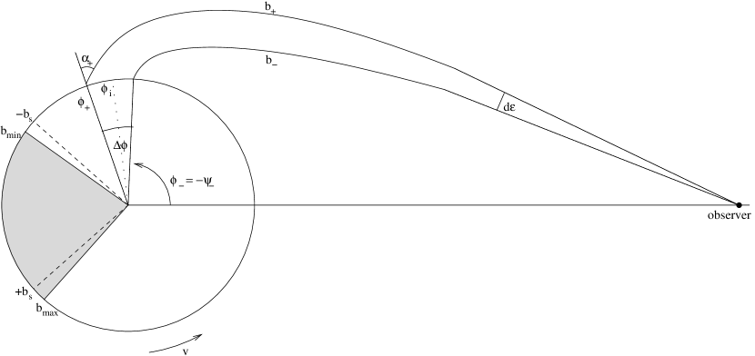
Figure 1.— Definition of angles.

2.3. Deflection of Photons

In Figure 1 we illustrate the deflection of photons from the point of emission on the star to the observer. We define the azimuthal location of the distant observer to be at $\phi=0$. A photon with impact parameter $b$ hits the observer if it was emitted at azimuthal angle $\phi_{i}$. The initial emission location is found by dividing Equation 9 by Equation 10, and integrating from the star’s surface to the distant observer:

$$-\phi_{i}(b)=\int_{\bar{r}_{e}}^{\infty}e^{\alpha-\frac{1}{2}(\gamma+\rho)}\frac{\omega(1-\omega b)+be^{2\rho}/\bar{r}^{2}}{\left((1-\omega b)^{2}-b^{2}e^{2\rho}/\bar{r}^{2}\right)^{1/2}}\,\mathrm{d}\bar{r}.$$ (13)

The deflection angle $\psi$ is defined by $\psi=-\phi_{i}$. In the calculation of flux from a star, both the quantities $\psi(b)$ and $\mathrm{d}\psi/\mathrm{d}b$ are of importance. These quantities are plotted for the fiducial stellar model in Figure 2. In addition, we show the deflections for the SE static model. The differences between the calculations with and without rotation are very small. The worst errors occur at the limbs of the star, so these differences are only likely to be of importance if the light is preferentially emitted in directions close to the horizontal.

Figure 2.— Bending angle and its derivative as a function of impact parameter for Model 4, calculated using the full metric and the SE metric.

2.4. Times of Arrival

To accurately model pulse shapes, we account for the different amounts of coordinate time that photons emitted from different regions of the star will take to reach the observer. Once the times of arrival (TOA) are known, the photons can be placed into the correct detector timing bins. The choice of zero time is arbitrary, so we have chosen a value of zero TOA for a photon with zero impact parameter. For photons emitted with the maximal values of impact parameter, the TOA is similar to the light travel time across the star. For our fiducial stellar model with $R=16.38$ km, the light travel time is close to 80 $\mu$s. Compared to a spin period of 1.6 ms, this corresponds to a 5% effect, which will be seen to have a significant effect on the calculated pulse shapes.

The TOA is calculated by dividing Equation 8 by Equation 10, integrating from the star’s surface to the distant observer and then subtracting off the corresponding quantity for a $b=0$ photon. This yields the TOA formula

$$\mathrm{TOA}(b)=\int_{\bar{r}_{e}}^{\infty}e^{\alpha-\frac{1}{2}(\gamma+\rho)}\left(\frac{(1-\omega b)\bar{r}}{\left((1-\omega b)^{2}\bar{r}^{2}-b^{2}e^{2\rho}\right)^{1/2}}-1\right)\,\mathrm{d}\bar{r}.$$ (14)

In Figure 3 we plot the TOA for our fiducial star and the SE static star. Note that in the full rotational calculation, the retrograde photon takes longer to reach the observer than the prograde photon. This is due to the frame-dragging effect. The magnitude of this effect is about $1/10$ of the effect due to the light-crossing time in the corresponding SE models so we expect that for most timing applications that it will not be detectable.

Figure 3.— Times of arrival (TOA) as a function of bending angle for Model 4, calculated using the full metric and the SE metric.

2.5. Redshift

In our units, the photon’s energy as measured by an observer far from the star has been normalized to unity. As a result, any other observer with four-velocity $u^{a}$ measures a photon energy of $E_{u}=-\ell^{a}u_{a}$, where the photon’s four-velocity components $\ell^{a}=\mathrm{d}x^{a}/\mathrm{d}\lambda$ are given in Equations 8–10. The star’s four-velocity at the equator is

$$u^{a}=\frac{1}{V}\left(t^{a}+\Omega_{\star}\phi^{a}\right),$$ (15)

where $\Omega_{\star}$ is the star’s angular velocity as measured by an observer at infinity, and the normalization condition $u^{a}u_{a}=-1$ yields

$$V^{2}=e^{\gamma+\rho}\left(1-(\Omega_{\star}-\omega)^{2}\bar{r}^{2}e^{-2\rho}\right),$$ (16)

where all quantities are evaluated on the star’s equator.

The redshift factor $(1+z)$ between light emitted at the star’s equator and detected by an observer at infinity is

$$1+z=e^{-\frac{1}{2}(\gamma+\rho)}\frac{(1-\Omega_{\star}b)}{\sqrt{1-(\Omega_{\star}-\omega)^{2}\bar{r}^{2}e^{-2\rho}}}.$$ (17)

Note that the quantity $v_{\mathrm{ZAMO}}^{2}\equiv(\Omega_{\star}-\omega)^{2}\bar{r}^{2}e^{-2\rho}$ appearing in the denominator is the square of the velocity of the star’s fluid as measured by an observer with zero angular momentum; i.e., an observer with $u_{\phi}=u^{r}=u^{\theta}=0$.

2.6. Zenith Angle

If the radiation is not emitted isotropically, the intensity will depend on the initial direction of the photon with respect to the fluid. The angle between the local normal to the star’s surface and the direction in which a photon is emitted is the zenith angle and will be denoted $\alpha$. This angle depends on the frame in which it is measured. For example, consider the co-moving observer at the equator with four-velocity given by Equation 15. In order to define this angle in an invariant manner, we first define the spatial projection operator $h_{ab}$ for the co-moving observer as:

$$h_{ab}\equiv g_{ab}+u_{a}u_{b}.$$ (18)

Any photon’s four velocity $\ell^{a}$ can then be decomposed into a “time” component $\ell^{u}=-\ell^{a}u_{a}=(1+z)$ and a “spatial” component $\ell_{\perp}^{a}=\ell^{b}h^{a}_{\;b}$ using the spatial metric. For all photons, the spatial components satisfy the normalization condition $|\ell_{\perp}|=\ell^{u}$.

The unit normal to the fluid $n^{a}$ (in the equatorial plane) as measured by the co-moving observer has only a radial component $n^{r}=e^{-\alpha}$. The co-moving observer measures an angle of $\alpha_{e}$ between the photon and the normal, defined by the equation

$$\cos\alpha_{e} = \frac{h_{ab}\ell_{\perp}^{a}n^{b}}{\ell^{u}}$$ (19)

$$= \left((1-\omega b)^{2}-\frac{b^{2}}{\bar{r}^{2}}e^{2\rho}\right)^{1/2}\frac{\sqrt{1-(\Omega_{\star}-\omega)^{2}\bar{r}^{2}e^{-2\rho}}}{(1-\Omega_{\star}b)}.$$

It will also be useful for us to know what the non-rotating observer with $u^{a}\propto t^{a}$ at the surface of the star measures for the angle formed by the photon and the normal; following the same procedure, this angle is

$$\cos\alpha_{o}=\left((1-\omega b)^{2}-\frac{b^{2}}{\bar{r}^{2}}e^{2\rho}\right)^{1/2}\sqrt{1-\omega^{2}\bar{r}^{2}e^{-2\rho}}.$$ (20)

2.7. Angles between Photons

In a more general calculation of flux from a two-dimensional emitting area on the star, we would need to calculate the solid angle subtended by the area, as viewed by the observer at infinity. In this paper, we are only including the flux of photons emitted from a segment of the equator into the equatorial plane. Adopting this special one-dimensional emission region means that observed radiation will subtend zero solid angle in the observer’s sky. The most straightforward way of adjusting the usual definition of flux for this simplified emission region is to define flux in terms of an integral over angle in the observer’s one-dimensional “sky” which coincides with the equatorial plane.

In Figure 1 we show a curve of angular extent $\Delta\phi$ on the star, and the angle measured by the observer at infinity between the two photons emitted from the end-points (points $\phi_{-}$ and $\phi_{+}$) is $\mathrm{d}\varepsilon$. If the impact parameters for these two photons are related by $b_{+}=b_{-}+\mathrm{d}b$, the angle observed between the two photons reduces at infinity to

$$\mathrm{d}\varepsilon=\frac{\mathrm{d}b}{r},$$ (21)

if both photons are restricted to move only in the equatorial plane. This result is familiar from the usual Schwarzschild metric; its validity for the current case is demonstrated in the Appendix.

2.8. Outline of Numerical Method

We now outline the procedures used to compute pulse shapes from a rotating neutron star when the photons and the observer are restricted to the equatorial plane. We discretise the period of the star’s rotation into $N_{t}$ bins and keep track of bins of flux $F_{i}$, and bins of detector integration time $T_{i}$, where $i$ indicates the period bin in which the flux is received. The angular size of the emission region $\Delta\phi$ is related to the number of period bins by $\Delta\phi=2\pi/N_{t}$. The centre of the emission region at each step is $\phi_{i}=(i-1)(\Delta\phi)$. Figure 1 shows the relevant quantities.

We obtain the binned fluxes $F_{i}$ by performing the following steps at each period step $i$:

1. Calculate the impact parameters of the null rays arriving at the observer from $\phi_{-}=\phi_{i}-(\Delta\phi)/2$, $\phi_{i}$, and $\phi_{+}=\phi_{i}+(\Delta\phi)/2$. Denote these impact parameters by $b_{-}$, $b$, and $b_{+}$. This is done by numerically solving Equation 13.

2. Calculate the redshift $z(b)$ using Equation 17.

3. Calculate the zenith angle $\alpha_{e}(b)$ using Equation 19.

4. Calculate the angular contribution to the flux integral, $\mathrm{d}\varepsilon$, using Equation 21.

5. Calculate the TOAs for the limbs, $\mathrm{TOA}(b_{-})$ and $\mathrm{TOA}(b_{+})$, expressed in units of the rotation period of the star, and $\Delta T=|\mathrm{TOA}(b_{-})-\mathrm{TOA}(b_{+})|$ . This is done via Equation 14.

6. Convert the TOAs of the limbs to indices of the flux binning. This is done, schematically, by computing $j_{\pm}=\mathrm{floor}(i+(N_{t})(\mathrm{TOA}(b_{\pm})))$, where $j_{\pm}$ is the bin corresponding to the arrival time of the flux corresponding to $b_{\pm}$.

7. If $j_{+}\neq j_{-}$, the flux from the limbs arrives during different period bins, and one needs to calculate the fractional amount of flux to be assigned to each bin, $x_{\pm}$, with $x_{+}+x_{-}=1$.

8. Calculate the flux integral

   $$F_{\mathrm{(1-D)}}=\int_{(1+z)\nu_{o_{\mathrm{low}}}}^{(1+z)\nu_{o_{\mathrm{high}}}}\mathrm{d}\nu_{\mathrm{e}}\int\mathrm{d}\varepsilon\,I_{\nu_{e}}(\alpha_{e})/(1+z(b))^{4},$$ (22)

   where $\nu_{o_{\mathrm{low}}}$ and $\nu_{o_{\mathrm{high}}}$ correspond to the lower and upper limits of the detector’s energy band. Note that this integral is a non-standard definition of flux which we must adopt because we are dealing with a special one-dimensional emission region, as discussed in Section 2.7; the observer only receives photons from within the equatorial plane (the sky is effectively one-dimensional), so the integral is over a one-dimensional angle, not the usual solid angle for a two-dimensional sky. This integral simplifies in the case of bolometric flux since the integral will be over all energies at each step. Since the angle $\mathrm{d}\varepsilon$ corresponds to an angle between photons arriving at different times, this corresponds to the energy deposited in the detector in the time period $\Delta T$. This flux is then portioned into the flux bins $F_{j_{\pm}}$ using $F$ and $x_{\pm}$.

9. The bins of integration time $T_{j_{\pm}}$ are incremented by $(\Delta T)x_{\pm}$.

Once the calculation for each period step is completed, the non-zero bins of flux $F_{i}$ are weighted by dividing by the corresponding integration time $T_{i}$. This step is necessary because without this weighting the fluxes in each bin do not necessarily correspond to uniform intervals of integration time by the detector.

The fluxes $F_{i}$ correspond to the pulse shape for an infinitesimal spot of angular size $\Delta\phi$. To investigate the pulse shapes of wider spots of width $k(\Delta\phi)$ we can compute the new pulse shape $P_{i}$ by

$$P_{i}=\sum_{j=0}^{k}F_{(i-k/2)+j},$$ (23)

where the values $F_{i}$ are understood to be periodic in the index $i$. Choosing the offset $(i-k/2)$ above is arbitrary; this choice keeps the spot initially centred as far as possible on $\phi=0$.

The rns code calculates the metric potentials to a finite value of $\bar{r}$, and so our calculation is performed at distant $r\approx 10^{10}$ cm and not at infinity. We have fully accounted for the very small corrections to the expressions appearing in Section 2 which result from not locating our observer at infinity.

In Figure 4 the bolometric pulse shapes computed using this algorithm are shown for the four model stars. In these calculations, the spot size is 0.25° for the 300 Hz models, and 0.5° for the 600 Hz models; these choices were made so that the bin widths for these cases corresponded to equal intervals of time. The general effect of rotation is to create an asymmetry in the pulse shape that increases as the rotational velocity increases. We have normalized all flux to the peak flux, and the moment the emission region becomes visible is defined to be the start of the period. We have broken each pulse into four time periods: the rise time, the fall time, the total time on and the total time off. These periods are listed in Table 2.

Figure 4.— Bolometric pulse shapes for the four model stars. The beginning of the rise for each pulse has been aligned with Phase = 0.

Table 2Timing of Bolometric Pulse Shapes

Model	Period	Rise	Fall	On	Off	$t_{\mathrm{rise}}/t_{\mathrm{fall}}$
1	3333.3	983.8	1511.6	2495.4	838.0	0.65
2	1666.7	377.3	868.1	1245.1	421.3	0.43
3	3333.3	719.9	1342.6	2062.5	1270.8	0.54
4	1666.7	231.5	787.0	1018.5	648.1	0.29

Note. — All times are in $\mu\mathrm{s}$, and pulse shape parameters are given to $\pm 2.3\,\mu\mathrm{s}$, corresponding to the width of one period bin.

In Table 2 it can be seen that increasing the star’s compactness $M/R$ increases the fraction of time that the pulse is on. This is due to the gravitational bending of light increasing the fraction of the time that the spot is visible. This effect is almost independent of the star’s spin rate. The asymmetry between the rise and fall time of the pulse is shown by the column $t_{\mathrm{rise}}/t_{\mathrm{fall}}$ in Table 2. The rise time corresponds to time during which the spot first appears on the blueshifted limb to the time of peak intensity. The Doppler boosting effect shifts the phase of maximum intensity to the blue-shifted side of the star, so that the rise time takes less than half of the total time on. Increasing the speed increases the asymmetry, as can be seen by comparing Tables 1 and 2.

3. Approximate Methods for Pulse Shape Calculations

Approximate methods for pulse shape calculations involve approximating the spacetime containing the neutron star by a metric which is analytically known. For example, in the S+D approximation, light-bending and time-delays are calculated as though the star was not rotating, using the method described in Pechenick, Ftaclas, & Cohen (1983). Special relativistic effects are included by modeling the star as a rapidly-rotating object with no gravitational field. The photons’ redshifts are computed by combining the Schwarzschild gravitational redshift with the special relativistic Doppler effect. This approximate approach is attractive since the gravitational field is completely described by the Schwarzschild metric, for which simple formulae exist. The S+D approximation has been described in detail by Poutanen & Gierliński (2003), so only a brief outline of the method will be given here. However, it should be noted that Poutanen & Gierliński (2003) do not include time-delays due to different light travel times from different parts of the star. In Section 3.1, we show how the method employed by Poutanen & Gierliński (2003) can be recovered from the more general case of Section 2 by taking appropriate limits.

An alternative, but similar approximation is the use of the Kerr black hole metric to approximate the gravitational field of a rotating neutron star (Chen & Shaham, 1989; Braje, Romani, & Rauch, 2000; Bhattacharyya et al., 2004). While the gravitational fields outside of rotating neutron stars and black holes are not the same for arbitrarily fast rotation, the Kerr black hole is a reasonable approximation to a neutron star if it is spinning slowly. We expect that the Kerr metric is a reasonable approximation for stars with spin frequencies of 300 Hz, but at 600 Hz there would be large differences. These differences will be quantified elsewhere.

3.1. The Schwarzschild + Doppler Approximation

The S+D approximation seeks to treat the exterior spacetime of the neutron star as though it is described by the corresponding SE spacetime. Effects due to the relative velocity of the star and observer are put in by hand. Consider the SE spacetime described by the potentials $\alpha$, $\gamma$ and $\rho$, with $\omega=0$, where the relationship of the potentials to the star’s mass and radius is given in Equations 3–5. We imagine that the matter comprising the star is still rotating, but take the Schwarzschild metric to be an approximation of the exterior spacetime. Denote the Schwarzschild redshift as $z_{s}$ so that

$$1+z_{s}=\frac{1}{\sqrt{1-2M/R}}.$$ (24)

Using Equation 3, we see that the factor of $\exp{-(\gamma+\rho)/2}$ reduces to $1+z_{s}$. The equatorial velocity of the star measured in the SE spacetime of Equation 6 can be written, via Equation 4, as $v_{eq}=\Omega_{\star}\bar{r}\exp(-\rho)$. Introducing the function

$$\eta\equiv\frac{\sqrt{1-v_{eq}^{2}}}{1-\Omega_{\star}b},$$ (25)

we see that the Schwarzschild case ($\omega\rightarrow 0$) of the exact redshift expression in Equation 17 is given by

$$\lim_{\omega\rightarrow 0}(1+z)=\frac{(1+z_{s})}{\eta},$$ (26)

so that $\eta$ plays a role similar to the Doppler boost factor in special relativity with no gravitational field present.

Now we express $\eta$ in terms of the zenith angle of Section 2.6. As measured by the co-moving observer and the static observer, these angles are respectively

$$\lim_{\omega\rightarrow 0}\cos\alpha_{e}=\eta\sqrt{1-\frac{b^{2}}{R^{2}}\left(1-\frac{2M}{R}\right)},$$ (27)

and

$$\lim_{\omega\rightarrow 0}\cos\alpha_{o}=\frac{1}{\eta}\lim_{\omega\rightarrow 0}\cos\alpha_{e}=\sqrt{1-\frac{b^{2}}{R^{2}}\left(1-\frac{2M}{R}\right)}.$$ (28)

Equation 28 is a quadratic equation for $b$ in terms of $\alpha_{o}$ with the solution

$$b=\pm\frac{R}{\sqrt{1-2M/R}}\sin\alpha_{o},$$ (29)

where the plus/minus sign corresponds to co- and counter-rotating photons. If we know the angle $\alpha_{o}$ for a given photon, and solve for the corresponding $b$ via Equation 29, then using the definition of $\eta$ from Equation 25 and our expression for velocity in the SE spacetime from Equation 6, we have that

$$\eta=\frac{\sqrt{1-v_{eq}^{2}}}{1\mp v_{eq}\sin\alpha_{o}}.$$ (30)

This is the usual Doppler factor for redshift without a gravitational field present. This formula, as well as the relationship between $\alpha_{e}$ and $\alpha_{o}$ in Equation 28, agree with the corresponding formulae used by Poutanen & Gierliński (2003) once it is noticed that they respectively denote our angles $\alpha_{e}$ and $\alpha_{o}$ by $\alpha^{\prime}$ and $\alpha$, and that the four-velocity of the fluid is perpendicular to the normal in the observer’s frame. The overall redshift, Equation 26, is just the product of the Doppler factor arising from emission in the co-moving frame into the observer’s frame at the surface, and the Schwarzschild gravitational contribution to redshift as the photons travel to infinity.

Finally, we turn our attention to the matter of time-delays. One is left with the choice of accounting for the contribution of time delays according to the method described in Section 2.8, or else simply calculating flux directly as a function of the emitting region’s location. If we elect to do the latter, we can still account for the special relativistic “snapshot” effect; this effect arises because the image in the detector at a given instant is formed by photons emitted at different times from different parts of the star. These corrections are put in by hand, making use of the conformality of the Lorentz transformations discussed by Terrell (1959). The main effect of special relativity on an area element of the star is that the observed shape is not changed, but the element will be magnified if it is moving away from the observer. As discussed by Poutanen & Gierliński (2003), the net result is that in the S+D approximation, the solid angle must be calculated using the formula

$$\mathrm{d}\Omega_{S+D}=\eta\,\mathrm{d}\Omega_{o}=\eta\,b\,\mathrm{d}b\,\mathrm{d}\phi/r^{2},$$ (31)

where $\mathrm{d}\Omega_{o}$ is the uncorrected element of solid angle. Note that such a correction need not be applied to the solid angle element when the flux is calculated using the method of Section 2.8 as this method accounts for all effects due to time-delay, i.e., the snapshot effect and the light-crossing time, by correctly binning the flux emitted by a region of constant angular size. To be clear, when we say a calculation “includes time-delay effects,” we mean in the sense of Section 2.8; calculations that do not include these time-delay effects have the special relativistic Doppler correction applied instead.

Since our emitting area is actually one-dimensional, we need to derive the analogue of the S+D solid angle element for one dimension. The calculation for one dimension yields the same Doppler boost factor,

$$\mathrm{d}\varepsilon_{S+D}=\eta\,\mathrm{d}b/r=\eta\frac{\mathrm{d}\psi}{r\,\mathrm{d}\psi/\mathrm{d}b},$$ (32)

where $\mathrm{d}\psi/\mathrm{d}b$ should be evaluated using the Schwarzschild metric and the angle $\mathrm{d}\psi$ is the constant angular size of the spot.

3.2. Comparison of Methods

We have computed pulse shapes in the S+D approximation for our fiducial star, Model 4. All calculations are for bolometric flux and the same angular emission sizes as in Section 2.8. We show pulse shapes in Figure 5 for four different calculation methods: Method I is the full general relativistic calculation described in Section 2. Method II is similar to Method I, but the time-delay binning is not performed and the special relativistic correction for the snapshot effect is included instead. Method III is the S+D approximation including time-delay effects. Method IV is the S+D approximation without time-delay effects.

In Table 3 we show the rise, fall, on and off times for the pulses computed with these methods. Typically, the differences between the full GR calculation and the S+D approximation is very small, amounting to only a few $\mu$s. The differences between methods that include or do not include time-delay effects is about an order of magnitude larger. The inclusion of time-delays keeps the total on or off time the same within a few $\mu$s, but decreases the rise time by 50 $\mu$s and increases the fall time by a similar amount. This corresponds to a change of about 20% in the rise time, which is a resolvable amount.

Table 3Bolometric Pulse Shapes Using Different Calculation Methods

Method	Rise	Fall	On	Off	$t_{\mathrm{rise}}/t_{\mathrm{fall}}$
I (Full GR, with TD)	231.5	787.0	1018.5	648.1	0.29
II (Full GR, without TD)	263.9	747.7	1011.6	655.1	0.35
III (SE Model, with TD)	233.8	775.5	1009.3	657.4	0.30
IV (SE Model, without TD)	268.5	740.7	1009.3	657.4	0.36

Note. — Comparison of timing parameters describing bolometric pulse shapes from different calculation methods, using Model 4 (Period = 1.6667 ms). Times are given to $\pm 2.3\,\mu\mathrm{s}$, corresponding to the width of one period bin.

Table 4Blackbody Soft-Hard Phase Lag Using Different Calculation Methods

Method	Phase Lag ($\pm 1/720$ (phase/$2\pi$))	Time Lag ($\pm 2.3\,\mu\mathrm{s}$)
I (Full GR, with TD)	0.020833	34.7
II (Full GR, without TD)	0.020833	34.7
III (SE Model, with TD)	0.020833	34.7
IV (SE Model, without TD)	0.019444	32.4

Note. — Comparison of soft/hard phase lag for unbeamed blackbody emission for Model 4 (Period = 1.6667 ms) for different calculation methods. Radiation temperature $kT$ = 1 keV; soft band is 3–5 keV; hard band is 5–7 keV.

Figure 5.— Bolometric pulse shapes for Model 4 using different calculation methods.

The total time on is not changed much by the inclusion of time-delays since the asymmetry caused by frame-dragging is quite small. However, including time-delays increases the asymmetry between the rise and fall times. This effect enters because the beginning of the pulse corresponds to the moment when the spot is at the limb, where the time-delay is largest. However, the peak intensity corresponds to a moment when the spot is relatively close to the observer, so the time delay is very small. This effectively delays the beginning of the pulse, but not the time of peak intensity, increasing the rise/fall asymmetry. This can have important consequences if the pulse shape is fitted using a method that doesn’t include time-delays, since all pulse asymmetry will be incorrectly attributed to the rotation speed.

4. Effects Due to the Emission Region

We now consider the sensitivity of the pulse shapes to various properties of the emitting region. The different properties considered are the emission spectrum, beaming, and the angular size of the emitting region (“spot size”). Unless otherwise indicated, our calculations are for the fiducial star (EOS L, 600 Hz) using Method I, i.e., using the exact metric with time-delay effects.

We computed the phase lag of soft X-rays relative to hard X-rays if two detectors sensitive to different energy bands observe a blackbody. We chose a blackbody of 1 keV, a soft band of 3–5 keV, and a hard band of 5–7 keV in order to investigate this effect. In Figure 6 we show the hard and soft pulse shapes computed using Methods I and II for the fiducial star; the same pulse shapes computed using Methods III and IV nearly overlap these curves. The peak of soft X-ray flux arrives after the peak of the hard X-ray flux; this phase lag was calculated using all methods and is shown in Table 4. The lag is independent (within error) of the calculation method, although the individual pulse shapes do depend on the calculation method.

Figure 6.— Pulse shapes in hard and soft bands for blackbody emission using different calculation methods.

Next we consider the effect of beaming. We consider infinitesimal spots which have different beaming functions and show the bolometric flux. We show the cases of

1. isotropic emission;

2. fan beaming, $I\propto 1-\cos\alpha_{e}$;

3. pencil beaming, $I\propto\cos^{4}\alpha_{e}$; and,

4. Gaussian beaming, $I\propto\exp(-\sin^{2}\alpha_{e}/2\sigma^{2})$ with $\sigma=0.1$.

Figure 7 shows these four pulse profiles. As the beaming toward the normal increases, the peak intensity arrives later since the light is emitted when the spot is closest to the observer. Hence, an emission region composed of two components with different types of beaming will exhibit phase lags which can be larger than the Doppler lags in energy.

Figure 7.— Bolometric pulse shapes for beamed emission using Model 4.

The effect of a larger spot with uniform brightness and no beaming is shown in Figure 8. Not surprisingly, the larger the spot size, the broader the peak intensity.

Figure 8.— Bolometric pulse shapes for larger emitting regions using Model 4.

5. Estimation of Errors in Fitting Radius

We wish to estimate the error in fitting the radius of the star using the S+D approximation. To do this, we generated bolometric flux pulse shapes for the following cases using Method I:

1. Models 1, 2, 3, 4: isotropic emission, infinitesimal spot;

2. Models 1, 2, 3, 4: $I\propto 1-\cos\alpha_{e}$ emission, infinitesimal spot;

3. Models 3, 4: isotropic emission, 30° spot; and,

4. Models 3, 4: $I\propto 1-\cos\alpha_{e}$ emission, 30° spot.

To these we fit pulse shapes for one-dimensional emission from an infinitesimal region calculated using the S+D approximation without time-delays together with either the light-bending approximation of Beloborodov (2002) or the exact light-bending formula of Equation 13 to obtain a fitted radius. The fits performed with the exact light-bending formula can be considered as a similar method to that employed by Poutanen & Gierliński (2003) for fitting observations of SAX J1808.4-3658 to obtain a fitted radius; however, our method is specific to the one-dimensional flux we defined in Section 2.8 for emission and observation restricted to the equatorial plane. The results are summarised in Table 5 for the fits using approximate light-bending, and Table 6 for the fits using exact light-bending. The quality of the fits were generally good for the cases of isotropic emission, and the fits were quite poor for the fan beam emission. To understand the poor quality of these fits, note that for fan beam emission most of the flux is recorded when the emitting region is near the limbs of the star, so the effects due to time-delays are significant; another effect is the poor performance of the light-bending approximation at these locations (Beloborodov, 2002), but an examination of the results in Tables 5 and 6 indicates that this is a comparatively small effect on the quality of fit. It is also worth noting that good fits do not necessarily imply good performance in obtaining the true radius; for example, the isotropic Model 1 calculation with approximate light-bending performs quite poorly at obtaining the radius, while the fit was relatively good.

Table 5 Fits to Radius Using Approximate Light-Bending Formula

Method	Model	Emission	Spot Size	Fitted Radius (km)	Percent Error	$\mathrm{S.Sq.}/N$ $(\times 10^{-4})$
I	1	isotropic	0.25°	10.517	$+9.3$	0.72
	2		0.5°	10.344	$+5.7$	0.38
	3		0.25°	15.646	$+3.6$	0.045
	4		0.5°	16.747	$+2.2$	3.2
II				16.463	$+0.5$	0.14
III				16.788	$+2.5$	2.8
IV				16.358	$-0.1$	0.25
I	1	$I\propto 1-\cos\alpha_{e}$	0.25°	10.348	$+7.6$	34
	2		0.5°	10.744	$+9.8$	67
	3		0.25°	15.456	$+2.3$	36
	4		0.5°	17.765	$+8.5$	59
	3	isotropic	30°	15.045	$-0.4$	0.82
	4			15.68	$-4.3$	2.3
	3	$I\propto 1-\cos\alpha_{e}$	30°	14.495	$-4.1$	42
	4			14.783	$-9.7$	55

Table 6 Fits to Radius Using Exact Light-Bending Formula

Method	Model	Emission	Spot Size	Fitted Radius (km)	Percent Error	$\mathrm{S.Sq.}/N$ $(\times 10^{-4})$
I	1	isotropic	0.25°	9.70	$+0.8$	0.44
	2		0.5°	9.975	$+2.0$	2.7
	3		0.25°	15.19	$+0.5$	0.50
	4		0.5°	16.85	$+2.9$	4.8
	1	$I\propto 1-\cos\alpha_{e}$	0.25°	9.73	$+1.1$	24
	2		0.5°	10.28	$+5.1$	56
	3		0.25°	14.98	$-0.8$	32
	4		0.5°	17.66	$+7.8$	58
	3	isotropic	30°	14.44	$-4.4$	0.61
	4			15.71	$-4.1$	3.0
	3	$I\propto 1-\cos\alpha_{e}$	30°	13.93	$-7.8$	33
	4			14.51	$-11.4$	49

Considering the Method I cases with an infinitesimal spot in both sets of fits, the radius is generally overestimated by up to 9.8%, with the exception of the fit to the fan-beam case for Model 3 calculated with exact light-bending, where the result was a poor quality fit underestimating the radius by 0.8%. The tendency to overestimate the radius is a result of the fits ignoring the time-delay effect, so that all asymmetries between the rise and fall time ($t_{\mathrm{rise}}/t_{\mathrm{fall}}$ in Tables 2 and 3) are attributed to the equatorial speed of the star. This forces the fitting program to assume a larger speed and therefore a larger radius (since the spin frequency is fixed). Of the four models computed with isotropic emission Model 4 has the worst quality fit, which is not surprising since it was chosen to maximize the effects of rotation.

For the 30° emitting region, the fits underestimate the actual radius by up to 11.4%. The change in fit radius from the infinitesimal case is $-3.8$–$-17.8$%, which is in part cancelled by the positive error in all but one of the infinitesimal cases. More compact stars have light visible for a longer fraction of their period, and so the fit attempts to compensate for the effect of a large emitting region (which is visible for a longer fraction of the period) by making the star more compact.

We also performed fits with approximate light-bending to the pulse shapes for Model 4 calculated using Methods II, III, and IV for a 0.5° spot with both isotropic and fan beam emission; Table 5 shows the results for the isotropic cases. Methods I and II both use the exact metric, but Method II does not include time-delays. The difference between the fitted radii obtained for these methods is $0.3$ km for isotropic emission, and $1.3$ km for fan beam emission. Comparing the fitted radii for pulse shapes that differ only by the selection of the metric (SE or exact), the differences in the obtained radius ranged from $0.03$–$0.17$ km, depending on beaming and the inclusion of time-delay effects. In this case the largest effect on the fitted radius comes from the inclusion of time-delay effects, with the effect due to the metric approximation about an order of magnitude smaller. We expect the errors arising from the approximation of the metric to get larger for more compact models, i.e., softer EOS, as the frame-dragging effect can be larger for such stars, while the time-delay effects would get smaller owing to the shorter light-crossing time.

Finally, the error in the fitted radius obtained when we fit to the Model 4 pulse shape calculated using the S+D approximation without time-delays (Method IV) was $0.02$ km for isotropic emission and $0.1$ km for fan beam emission. This error arises only from the Beloborodov (2002) approximation for light-bending used by the fitting procedure.

Comparing the set of results using approximate light-bending in Table 5 to the results using exact light-bending in Table 6, it is clear that it is not uniformly true that fitting with the exact light-bending formula necessarily yields improved results, improved fit quality, or both. For example, the calculations for Model 4 with isotropic emission and an infinitesimal emission region is an example where the use of the exact light-bending formula actually yields a poorer fit to the radius, and a poorer quality of fit.

 

 

6. Conclusions

Observations of the pulse profile of light emitted from the surface of a neutron star have the potential to constrain the star’s mass, radius, and equation of state. Restricting ourselves to the case of light emitted and received in the equatorial plane of a rapidly-rotating neutron star, we have compared a variety of methods to calculate the pulse shapes observed by a distant observer; this restriction requires us to use a definition of flux adapted to the one-dimensional nature of the emitting region which was employed for all of our calculations. In particular, we have compared the use of an exact neutron star metric including a general relativistic treatment of all effects due to rotation, with the use of an associated Schwarzschild metric where the effects due to rotation of the star are put in by hand (the “Schwarzschild + Doppler” (S+D) approximation). For each of these cases we have either included the effects of time-delays by fully accounting for the times of arrival of photons from different locations on the star, or else neglected the totality of these effects and only applied a special relativistic Doppler correction to account for the so-called “snapshot” effect.

The time-delay effects which we are able to account for can be split into two classes: effects owing to the light-crossing time which are also present for static stars, and effects owing to frame-dragging which is present in an exact calculation of the neutron star spacetime. For our fiducial star, a 600 Hz, $1.4M_{\odot}$ neutron star with $R=16.38~{}\mathrm{km}$, accounting for the light-crossing time had the effect of decreasing the rise time and increasing the fall time of the calculated pulse by about 50 $\mu$s, which is about 20% of the rise time and is a resolvable amount. Effects due to frame-dragging in this case were about an order of magnitude smaller. While we found that the calculation method does change the pulse shape, we found that the calculation of the total lag between the peaks of flux in soft and hard X-rays for a simple blackbody emission spectrum did not strongly depend on the calculation method used.

Constraints on the stellar parameters are obtained by fitting theoretical pulse shapes to observations. We wished to determine whether a fitting routine which uses the S+D approximation without time-delay effects could accurately determine the parameters corresponding to pulse shapes calculated with all effects included. Using an exact treatment of photon propagation from an infinitesimal one-dimensional emission region, we created artificial light curves for a number of different neutron stars and equatorial emission types. We then attempted to fit these light curves using a code based on the S+D approximation without time-delays to obtain a fitted radius. We found for infinitesimal emission regions that fitting to the approximate pulse shapes tends to overestimate the stellar radius by up to 9.8%. On the other hand, fitting to a pulse shape for an emission region that is 30° wide has the effect of underestimating the radius by up to about 10%. Furthermore, the quality of these fits was quite poor in the case of emission which was preferentially emitted in the horizontal direction. These results should not be misconstrued as a claim that the analysis of SAX J1808.4-3658 observations by Poutanen & Gierliński (2003) is flawed since our calculations only provide a worst-case scenario. The X-ray pulsar SAX J1808.4-3658 rotates at a slower rate than our fastest neutron star model, and most likely emits its radiation from high latitudes where the S+D approximation should be more valid.

In this paper we have restricted our attention to photons emitted from the equator whose paths stay in the equatorial plane, mainly because the effects of rotation should be strongest for these photons. However, if the emission area is large and encompasses a wide range of latitudes on the star, we expect that the varying shape of the star will have an important effect. Rotation causes a star to become oblate, and the effective gravitational field at the poles is larger than at the equator. As a result, the static part of the gravitational redshift is larger at the poles than at the equator. In addition, light emitted near the poles will experience a greater gravitationally-induced time delay. We intend to explore the effect of rotation on pulses observed from spots and observers at a range of latitudes in a future publication.

Appendix A Derivation of the Observed Angle Between Photons

Equation 21 gives the infintesimal angle $\mathrm{d}\varepsilon$ formed by the world lines of two photons as measured by a static observer located in the equatorial plane at infinity. Let the two photons have four-velocities $\ell^{a}$ and $m^{a}$, with impact parameters $b_{+}$ and $b_{-}$, respectively. The angle is calculated as in Section 2.6: The oberserver has $u^{a}\propto t^{a}$, and we define the projection operator as $h_{ab}^{(\infty)}\equiv g_{ab}+u_{a}u_{b}$ and the magnitudes of the projected null vectors as $\ell^{u}\equiv|\ell_{\perp}|=|h_{ab}^{(\infty)}\ell^{b}|$. The angle is calculated by the inner product of the projected vectors:

$$\cos\varepsilon = \frac{h_{ab}^{(\infty)}\ell_{\perp}^{a}m_{\perp}^{b}}{\ell^{u}m^{u}}$$ (A1)

$$= \omega(b_{+}+b_{-})+b_{+}b_{-}\left(\frac{e^{2\rho}}{\bar{r}^{2}}-\omega^{2}\right)$$

$$+\sqrt{\left[(1-\omega b_{+})^{2}-\frac{b_{+}^{2}e^{2\rho}}{\bar{r}^{2}}\right]\left[(1-\omega b_{-})^{2}-\frac{b_{-}^{2}e^{2\rho}}{\bar{r}^{2}}\right]}.$$

This formula is only valid when the photons are restricted to move in the equatorial plane, i.e., $u^{\theta}=0$. To get the infinitesimal version of this equation, put $b_{+}=b_{-}+\mathrm{d}b$, and Taylor expand the left-hand side for small angles $\mathrm{d}\varepsilon$. Expanding the right-hand side in $\mathrm{d}b$ and equating the second-order terms gives:

$$\mathrm{d}\varepsilon^{2}=-\mathrm{d}b^{2}\left[(1-\omega b_{-})^{2}-\frac{b_{-}^{2}e^{2\rho}}{\bar{r}^{2}}\right]\left[\frac{\omega^{2}\bar{r}^{2}-e^{2\rho}}{\bar{r}^{2}\left(1-\omega b_{-}\right)^{2}-b_{-}^{2}e^{2\rho}}-\left(\frac{\omega^{2}b_{-}\bar{r}^{2}-b_{-}e^{2\rho}-\omega\bar{r}^{2}}{\bar{r}^{2}\left(1-\omega b_{-}\right)^{2}-b_{-}^{2}e^{2\rho}}\right)^{2}\right].$$ (A2)

In the large $\bar{r}$ limit, $\omega$ falls off as $1/\bar{r}^{3}$, so to leading order in $1/\bar{r}$ the first term in square brackets is $\sim 1$ and the second term in square brackets is $\sim-e^{2\rho}/\bar{r}^{2}$. So we have for large $\bar{r}$,

$$\mathrm{d}\varepsilon=\frac{e^{\rho}\mathrm{d}b}{\bar{r}},$$ (A3)

and in terms of the usual Schwarzschild $r$ coordinate given by Equation 4, this is

$$\mathrm{d}\varepsilon=\frac{\mathrm{d}b}{r},$$ (A4)

which is Equation 21.

References

- Arnett & Bowers (1977) Arnett, W. D., & Bowers, R. L. 1977, ApJS, 33, 415
- Beloborodov (2002) Beloborodov, A. M. 2002, ApJ, 566, L85
- Bhattacharyya et al. (2004) Bhattacharyya, S., Strohmayer, T. E., Miller. M. C., & Markwardt, C. B. 2004, astro-ph/0402534, ApJ, submitted.
- Braje, Romani, & Rauch (2000) Braje, T. M., Romani, R. W., & Rauch, K. P. 2000, ApJ, 531, 447
- Carter (1968) Carter, B. 1968, Phys. Rev., 174, 1559
- Chakrabarty & Morgan (1998) Chakrabarty, D. & Morgan, E. H. 1998, Nature, 394, 346
- Chen & Shaham (1989) Chen, K. & Shaham, J. 1989, ApJ, 339, 279
- Cui, Morgan & Titarchuk (1998) Cui, W., Morgan, E. H., & Titarchuk, L. G. 1998, ApJ, 504, L27
- Ford (1999) Ford, E. C. 1999, ApJ, 519, L73
- Ford (2000) Ford, E. C. 2000, ApJ, 535, L119
- Kapoor (1991) Kapoor, R. C. 1991, ApJ, 378, 227
- Kapoor & Datta (1986) Kapoor, R. C. & Datta, B. 1986, ApJ, 311, 680
- Kraus (2001) Kraus, U. 2001, ApJ, 563, 289
- Kraus et al. (2003) Kraus, U., Zahn, C., Weth, C.,& Ruder, H. 2003, ApJ, 590, 424
- Leahy (1990) Leahy, D. A. 1990, MNRAS, 242, 188
- Leahy (1991) Leahy, D. A. 1991, MNRAS, 251, 203
- Leahy & Li (1995) Leahy, D. A. & Li, L. 1995, MNRAS, 277, 117
- Leahy (2003) Leahy, D. A. 2003, ApJ, 596, 1131
- Leahy (2004) Leahy, D. A. 2004, MNRAS, 348, 932
- Leahy (2004b) Leahy, D. A. 2004b, ApJ, accepted
- Mészaros & Nagel (1985) Mészaros, P. & Nagel, W. 1985, ApJ, 299, 138
- Mészaros & Riffert (1988) Mészaros, P. & Riffert, H. 1988, ApJ, 327, 712
- Miller & Lamb (1998) Miller, M. C. & Lamb, F. K. 1998, ApJ, 499, L37
- Muno, Özel, & Chakrabarty (2002) Muno, M. P., Özel, F., & Chakrabarty, D. 2002, ApJ, 581, 550
- Nath, Strohmayer, & Swank (2002) Nath, N. R., Strohmayer, T. E., & Swank, J. H. 2002, ApJ, 564, 353
- Pechenick, Ftaclas, & Cohen (1983) Pechenick, K. R., Ftaclas, C., & Cohen, J. M. 1983, ApJ, 274, 846
- Poutanen & Gierliński (2003) Poutanen, J. & Gierliński, M. 2003, MNRAS, 343, 1301
- Scott et al. (2000) Scott, D., Leahy, D., Wilson, R. 2000, ApJ, 539, 392
- Stergioulas & Friedman (1995) Stergioulas, N. & Friedman, J. L. 1995, ApJ, 444, 306
- Terrell (1959) Terrell, J. 1959, Phys. Rev., 116, 1041
- Wang & Welter (1981) Wang, Y., Welter, G. 1981, A&A, 102, 97
- Weinberg, Miller & Lamb (2001) Weinberg, N., Miller, M. C. & Lamb, D. Q. 2001, ApJ, 546, 1098
- Wijnands & van der Klis (1998) Wijnands, R. & van der Klis, M. 1998, Nature, 394, 344