HETGS Spectroscopy of a Coronally Active Contact Binary, VW Cep

Abstract

Short-period binaries represent extreme cases in the generation of stellar coronae via a rotational dynamo. Such stars are important for probing the origin and nature of coronae in the regimes of rapid rotation and activity saturation. VW Cep ($P=0.28$ d) is relatively bright, partially eclipsing, and very active object. Light curves made from Chandra/HETGS data show flaring and rotational modulation, but no strong eclipses. Emission lines are broader than instrumental, indicating emission from both binary components. Velocity modulation of emission lines is indicative of geometric structure of the emitting plasma.

1 Introduction

VW Cep (HD 197433) is a W-type W UMa binary — a contact binary in which the more massive and larger star has lower mean surface brightness. The primary (deeper) photometric eclipse is the occultation of the smaller star. VW Cep has an 0.28 d (24 ks) orbital period. It is partially eclipsing ($i=63^{\circ}$), with component spectral types of K0 V and G5 V ([Hill1989], [Hendry & Mochnacki2000]). It is one of the X-ray-brightest of contact binaries.

Among the coronally active binaries, activity is strongly correlated with rotation ([Pallavicini1989]), but saturates at periods below one day ([Vilhu & Rucinski1983], [Cruddace & Dupree1984]). The trend has been referred to as “super-saturation” since instead of reaching a plateau, the activity level actually decreases with increasing rotation rate ([Randich1998], [Jardine & Unruh1999], [James et al.2000], [Stȩpień, Schmitt & Voges2001]). [Jardine & Unruh1999] argued that super-saturation occurs because loops are large and are unstable to the coriolis forces as they exceed the co-rotation radius: extended loops are swept to the poles. On the other hand, [Stȩpień, Schmitt & Voges2001] contended that loops are quite compact (relative to the stellar radius), but that the dynamics of surface flows in contact systems conspire to clear equatorial regions. The two scenarios are similar, but they differ in an important respect: X-ray sources are either low volume and dense, or large volume and rarefied. Optical light curve modeling is consistent with either (assuming correlation between photospheric spots and coronal emission); Doppler image maps of VW Cep ([Hendry & Mochnacki2000]) showed large polar spots.

[Choi & Dotani1998] have analyzed ASCA spectra, and found a flux of about $1\times 10^{-11}\,\mathrm{ergs\,cm^{-2}\,s^{-1}}$, and two component model temperatures of $7$ and $22\times 10^{6}$K ($\log T\sim 6.8$ and $7.3$) with about equal emission measures. They obtained significantly reduced abundances of Fe, Si, Mg, and O, but a Solar value for Ne. A flare also occurred during the observation, with a factor of three increase in the count rate. They used the flare emission measure and loop-scaling models to estimate a density of about $5\times 10^{10}\mathrm{cm^{-3}}$. The Ginga observations ([Tsuru et al.1992]) showed a thermal plasma temperature in excess of $10^{8}\,$K, a flux similar to that determined by [Choi & Dotani1998], no rotational modulation, and Fe K flux lower than expected.

2 High Resolution X-Ray Spectra

We observed VW Cep for 116 ks with the Chandra High Energy Transmission Grating Spectrometer (HETGS) on August 29-30, 2003 (observation identifier 3766). The instrument has a resolving power ($E/\Delta E$) of up to 1000 and wavelength coverage from about 1.5 Å to 26 Å in two independent channels, the High Energy Grating (HEG), and Medium Energy Grating (MEG).

VW Cep has also been observed in X-rays with the Chandra Low Energy Transmission Grating Spectrometer ([Hoogerwerf, Brickhouse & Dupree2003]), and with the XMM-Newton X-ray observatory ([Gondoin2004]). The only other contact binary observed with HETGS is 44 Boo ([Brickhouse, Dupree & Young2001]). Observations with the HETGS provide spectral resolution and sensitivity required to better determine line fluxes, wavelengths, and profiles. Ultimately, we wish to determine which coronal characteristics are truly dependent upon fundamental stellar parameters. Combination of VW Cep data with that from LETGS and XMM-Newton, as well as with results for other short period systems (e.g., 44 Boo, ER Vul) will help us to understand the basic emission mechanisms.

Here we concentrate on preliminary HETGS results. Data were calibrated with standard CIAO pipeline and response tools. Further measurements and analysis were done in ISIS ([Houck & Denicola2000]) and with custom code using ISIS as a development platform.

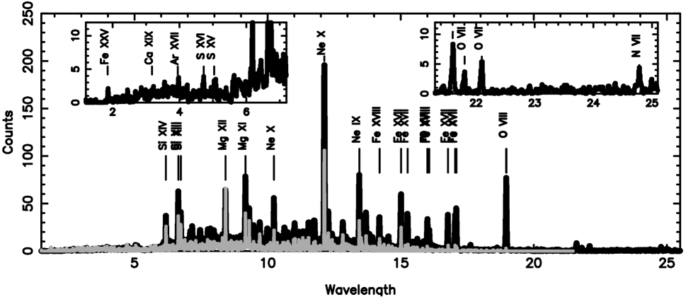
Figure 1: HETGS spectrum of VW Cep, 116 ks exposure. MEG (16433 counts) is the black line, and HEG (5269 counts) the gray. Insets show detail of the HEG spectrum (left) and MEG O VII triplet and N VII region (right).

3 The Spectrum

Figure 1 shows the counts spectrum obtained from the HETGS full exposure. The spectrum is qualitatively typical of coronal sources: a variety of emission lines from highly-ionized elements formed over a broad temperature region, from O vii, N vii, Ne ix, and Fe xvii ($\log T\sim 6.3$–$6.7$), up to high temperature species like S xv, S xvi, Ca xix (perhaps), and Fe xxv ($\log T\sim 7.2$–$7.8$). It is also apparent that iron has a fairly low abundance relative to neon, given the relative weakness of the 15Å and 17Å Fe xvii lines relative to the Ne ix 13Å lines. The observed flux in the 2–20 Å is $7\times 10^{-12}\,\mathrm{ergs\,cm^{-2}\,s^{-1}}$, and the luminosity (for a distance of 27.65 pc) is $6.5\times 10^{29}\,\mathrm{ergs\,s^{-1}}$.

Cursory inspection of the density-sensitive helium-like triplet lines (O vii, Ne ix, Mg xi) does not reveal ratios obviously far from their respective low-density limits.

4 Emission Measure

The differential emission measure ($DEM$) is a one dimensional characterization of a plasma, and can be defined as $N_{e}^{2}\,dV/dT$, in which $N_{e}$ is the electron density, $V$ is the emitting volume, and $T$ the temperature. The $DEM$ is an important quantity because it represents the radiative loss portion of the underlying heating mechanism. An emission measure can be derived from measurements of line fluxes and some assumptions about the homogeneity and ionization balance of the emitting plasma. Derivation of the emission measure thus relies on detailed knowledge of fundamental atomic parameters. Even given perfect knowledge of the ionic emissivities, their contribution functions versus temperature are broad so the emission integral cannot be formally inverted. Hence there are many methods to regularize the problem and solve for the emission measure and elemental abundances. For a first estimate, we use the simple method described by [Pottasch1963], in which the $DEM$ is approximated by a ratio of line luminosity to average line emissivity at the temperature of the maximum emissivity. Since there is a degeneracy in elemental abundance and $DEM$, the relative abundance of one element is scaled to bring their $DEM$ into better agreement with the locus of some other element with peak emissivities near the same temperatures (typically Fe, since it has many ions over a broad range in temperature).

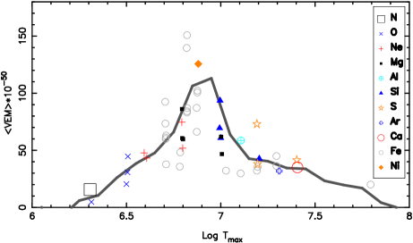
Figure 2: A provisional emission measure constructed from the ratio of line fluxes to mean emissivity over 0.3 dex. Points are plotted for each line used, and different elements points were scaled as a group to be roughly consistent with others. The solid line is a smoothed average of the individual points. The integrated emission measure is about $6.8\times 10^{52}\,\mathrm{cm^{-3}}$.

Figure 2 shows our provisional $DEM$, using the Astrophysical Plasma Emission Database (APED) for line emissivities ([Smith et al.2001]), the ionization balance of [Mazzotta et al.1998], and Solar abundances of [Anders & Grevesse1989]. There is large scatter in the values; the solid curve shows a smoothed average. There is sharp structure, with a fairly large peak at $\log T=6.9$. This $DEM$ can be used to generate a synthetic spectrum for further refinement of a plasma model. We found that with this distribution, we required a neon abundance of 1.0 (relative to Solar), and 0.3 for iron, confirming a trend already inferred from visual inspection of the spectrum. In iterative $DEM$ reconstruction techniques, sharper structure can be modeled than in the simple method. The fact that the simple method shows a strong peak hints at a highly structured $DEM$ in VW Cep.

5 Light and Phase Curves

Given the short orbital period, the observation covered almost five revolutions without interruption. Such phase redundancy is important to discriminate intrinsic variability from that caused by rotational or eclipse modulation. Figure 3 shows light curves in several wavelength regions and a hardness ratio. There was

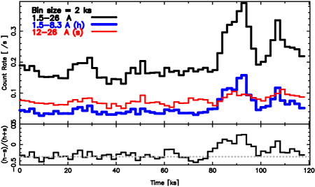
Figure 3: Count rates of VW Cep in 2 ks bins. In the upper panel are light curves extracted from all diffracted photons (1.5-26Å; upper heavy (black) curve), a “soft” band (12-26Å; lower, thinner curve (red) ), and a “hard” band (1.5-8.3Å; lower, thicker curve (blue)). The lower panel shows a hardness ratio (solid histogram), and the median of the hardness for the first 70 ks (light dotted line).

much variability. The hardness shows that the large increase near after 80 ks is a flare, by definition of being hotter: proportionally more flux was emitted at shorter wavelengths, which are very sensitive to high temperatures via the thermal continuum emission. Conversely, the bump in count rate between 20-30 ks does not show in hardness, and must be due to rotational modulation.

If we exclude the flare times and phase-fold the remaining data (about 3 orbital periods), we easily see the rotational modulation. Figure 4 shows this curve, using the ephemeris of [Pribulla et al.2002].

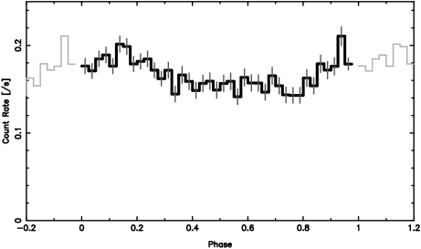
Figure 4: The phase-folded X-ray count-rate curve of VW Cep, excluding flare times. Bins are $\Delta\phi=0.025$, or 600 s, with a cumulative exposure per bin of 1800 to 2400 s, depending on the phase.

No eclipses are apparent, but instead, quasi-sinusoidal modulation of about 18%. The visual light curve ([Pribulla, Parimucha & Vanko2000]) shows a similar amplitude (16%), but is very different qualitatively, with strong minima at phases 0.0 and 0.5, and continuously variable in between (a trademark of W UMa systems). Without additional information, the X-ray light curve is not sufficient for localizing emission to one star or another. All we can say is that there is some asymmetric distribution, and possible occultation of large structures.

6 Velocity Modulation

Figure 5: Mean wavelengths of photons in the Ne x (12.1Å) region of the spectrum. The shaded area is the one-sigma envelope. Sinusoids are either radial velocities of the stellar centers of mass (black heavy curve: primary, “vrad1”; gray heavy curve: secondary, “vrad2”), or of points on opposing hemispheres of the primary (“vrot1A” and “vrot1B”). Sinusoids are approximate; they do not account for the tidal distortions of contact binaries.

In the high-resolution spectrum, additional information is available in the line shapes and centroids. The lines of VW Cep are broader than the instrumental resolution when integrated over the entire observation. This means that we are most likely sensitive to orbital Doppler shifts of one or both components, or to rotational broadening.

In order to investigate further, we have measured the mean wavelength of events in the best exposed line, Ne x (12.1Å), in phase bins of 0.1 (also excluding flare times). The one-sigma envelope is shown in Figure 5. It roughly follows the radial velocity of the primary (more massive) star (heavy dark sinusoid), except near phase 0.5, where it does a flip-flop, moving red-ward, then blue-ward. Our current hypothesis is that we are seeing a bias in the centroid during the transit of the secondary which first blocks the approaching limb of the primary, then the receding limb as the transit progresses. The dashed sinusoidal curves in the figure denote approximate photospheric rotational velocities on opposite sides of the primary. The velocity amplitude of a point on the stellar surface is consistent with the observed perturbation.

7 Conclusions and Future Work

The velocity curve of Ne x suggests that the emission is predominantly associated with the primary (larger, more massive) stellar component. This is also consistent with coincidence of the amplitude of the count-rate curve with the optical amplitude, and with the lack of a distinct primary eclipse (smaller, secondary star occulted). The velocity flip-flop perturbation also suggests that material is near the equatorial radius — either compact and near the equator itself, or extended at mid-latitudes, but co-rotating.

If the dip in rate seen by [Gondoin2004] in XMM-Newton data taken only 10 months earlier is really an eclipse, then this indicates rather large and rapid changes in coronal structure. The XMM-Newton observation, however, did not cover a full continuous period, and the dip is offset from phase 0.0, so the interpretation is difficult.

The line spectrum and crude $DEM$ reconstruction show that the the emission comes from a range of temperatures, and that the emission measure is highly structured. The relative abundances of Ne and Fe also appear to be similar to other coronal sources: Ne enhanced by a factor of a few relative to Fe.

In the future, we will perform a $DEM$ and abundance analysis, in which the line-based simultaneous $DEM$ and abundance solutions will be used to predict a better model continuum, and thereby improve line flux measurements, which are then used to iterate the model. We will also perform analysis of composite line profiles in order to refine the velocity versus phase analysis. By using a dozen or so lines, velocity sensitivity can be reduced to about $30\,\mathrm{km\,s^{-1}}$ (see [Hoogerwerf, Brickhouse & Mauche2004], for example). We will perform some analyses of the flare data separately to search for line shifts or flare occultation. And finally, we will do careful measurement and modeling of the density-sensitive He-like triplet ratios.