The VVDS data reduction pipeline: introducing VIPGI, the VIMOS Interactive Pipeline and Graphical Interface

The VIMOS VLT Deep Survey (VVDS), designed to measure 150,000 galaxy redshifts, requires a dedicated data reduction and analysis pipeline to process in a timely fashion the large amount of spectroscopic data being produced. This requirement has lead to the development of the VIMOS Interactive Pipeline and Graphical Interface (VIPGI), a new software package designed to simplify to a very high degree the task of reducing astronomical data obtained with VIMOS, the imaging spectrograph built by the VIRMOS Consortium for the European Southern Observatory, and mounted on Unit 3 (Melipal) of the Very Large Telescope (VLT) at Paranal Observatory (Chile). VIPGI provides the astronomer with specially designed VIMOS data reduction functions, a VIMOS-centric data organizer, and dedicated data browsing and plotting tools, that can be used to verify the quality and accuracy of the various stages of the data reduction process. The quality and accuracy of the data reduction pipeline are comparable to those obtained using well known IRAF tasks, but the speed of the data reduction process is significantly increased, thanks to the large set of dedicated features. In this paper we discuss the details of the MOS data reduction pipeline implemented in VIPGI, as applied to the reduction of some 20,000 VVDS spectra, assessing quantitatively the accuracy of the various reduction steps. We also provide a more general overview of VIPGI capabilities, a tool that can be used for the reduction of any kind of VIMOS data.

1 Introduction

Over the last few years the number of large telescopes available to the astronomical community has rapidly increased, together with the multiplexing capabilities of their instruments. While a normal long-slit spectrograph on a 4-meter class telescope could produce a few tens of spectra per night of observation, today a spectrograph like VIMOS at the VLT, or 2dF at the AAT, can obtain several thousands of spectra per night. This productivity increase has rendered obsolete traditional methods of data reduction and analysis, at least as long as these data must be reduced and analyzed in a timely fashion. It is clearly necessary to automatize as much as possible these operations, to increase the speed with which they can be carried out, but without sacrificing the capability of analyzing in detail the results of the various operations, and eventually manually intervene to change the way some of these operations are carried out. Moreover it is necessary to develop some efficient and rigorous data organizer and archiver, so that the available files and data would not be lost among hundreds or thousands of similar data and files. General-purpose astronomical software packages are not well equipped for these tasks, as witnessed by the ad-hoc data reduction pipelines developed for most large spectroscopic surveys, both in the case of multi-slit (see for example Colless et al. 1990 for the LDSS; Le Fèvre et al. 1995 for the CFRS) and multi-fiber observations (see for example Colless et al. 2001 for the 2dF; Stoughton et al. 2002 for the SDSS).

In particular, multi-fiber observations based surveys in the recent past have been very successful in processing large amount of spectroscopic data, but to their advantage was the fact that they were observing relatively bright galaxies at low redshift. Therefore the observations were carried out in the blue part of the optical spectrum, a wavelength domain contaminated by only a few strong sky emission lines. And the relative brightness of the observed galaxies makes the sky-subtraction process a non critical one, whereby the determination of the sky spectrum required only a few percent accuracy level. Significantly more challenging is the data processing task for a survey extending to higher redshift than that covered by the 2dF (Colless et al. 2001) and SDSS (Strauss et al. 2002) surveys. In this case it is necessary to derive spectra of very faint galaxies, with a surface brightness only a few percent of the sky one, and in the red part of the optical spectrum, a wavelength domain contaminated by many strong sky emission features. Early work in this challenging domain was provided by the CFRS team (Le Fèvre et al. 1995), but nowadays the high data throughput of 8-meter class telescopes require significant research and development efforts to obtain a spectroscopic data reduction pipeline capable of properly handling the data these telescopes are obtaining.

Among the last-generation spectrographs VIMOS is perhaps the most challenging in terms of data production, being currently the instrument with the highest multiplexing capabilites available to any astronomer. VIMOS is an imaging spectrograph mounted on the Unit 3 telescope (Melipal) of the Very Large Telescope (VLT) at the Paranal Observatory, in Chile (see Le Fèvre et al., 2000; 2002 for a detailed description of the instrument and its capabilities). It has been specially designed to be a survey instrument, and therefore its multiplexing capabilities have been pushed to the maximum: its field of view, divided in four separate quadrants, covers almost entirely the unvignetted area of the Nasmyth VLT focal plane, and during a single exposure, up to 1000 spectra can be obtained in MOS mode (6400 in IFU mode). Difficulties for the user in the data reduction process already begin when trying to find one’s way among the large number of raw science and calibration files, and increase going further along the reduction process, due to the number of calibrations and corrections that have to be applied to the data. To give an example, even just a single pointing in MOS mode, with its minimal set of calibration data (five bias, five flat field and one arc lamp exposure), is equivalent to 48 FITS files being produced (raw data only).

For this reason we were contracted by the European Southern Observatory (ESO) to deliver to them all the elements necessary to build a VIMOS-specific automatic data reduction pipeline. In collaboration with the ESO Data Management Division, we have therefore developed a C library of data reduction procedures, the VIMOS Data Reduction Software (DRS, see Scodeggio et al. 2000), which is now being used for the on-line reduction of VIMOS data at ESO. Because of its on-line usage, this ESO pipeline must work in a completely automatic fashion, but while this is an optimal choice to obtain a quick quality assessment for VIMOS observations, it is a far less acceptable one for a careful and complete science data reduction pipeline. Faced with the task of reducing some 100,000 spectra observed as part of the VLT VIMOS Deep Survey (VVDS, see LeFèvre et al. 2004 for a detailed description of the survey), we have used the DRS to produce a semi-automatic data reduction pipeline, the VIMOS Interactive Pipeline and Graphical Interface (VIPGI). With VIPGI we have kept the DRS capability for a very fast data reduction process, but we also have added many data reduction quality control points, a user friendly graphical interface, and a simple but effective method to organize the raw and reduced data.

VIPGI was designed specifically to carry out the reduction of the VVDS data, and its performance while performing this task is the focus of this paper. But VIPGI capabilities are far more general. It can be used to reduce VIMOS data of any kind, and not only MOS data. In particular, it can be used to reduce VIMOS IFU data, a task far more complex than the relatively simpler reduction of MOS data, and which is described in detail in a separate paper (Zanichelli et al. 2004). But VIPGI capabilities are general enough, at least as far as MOS data are involved, that it could be used as a generic pipeline tool for the reduction of MOS data from any spectrograph, and work is already under way to develop this functionality (see Paioro et al. 2004). So far VIPGI has been extensively tested while reducing more than 20,000 MOS spectra for the VVDS, and a smaller number of MOS and IFU spectra from other, independent projects. At the moment it is not publicly released, but it can be used either in Milano (Italy) or Marseille (France) by members of the ESO community under the supervision of a VIRMOS Consortium astronomer, who can provide guidance on how to handle non standard situations.

In this paper we discuss some of VIPGI general concepts (sections 2 and 3), and then focus on the reduction of VVDS MOS data, and the quality of the final VVDS spectra (sections 4 and 5). The data organizer and the data browsing and plotting facilities are briefly described in sections 6 and 7.

2 The VIMOS Interactive Pipeline and Graphical Interface

The core of the VIPGI pipeline is composed of a set of routines performing the data reduction, coded using the C language to obtain the maximum speed for this computationally intensive task. Routines range from the basic ”opening a file and reading its content” to wavelength calibration, spectral extraction and IFU 3D data cube reconstruction, and are organized in a relatively small number of reduction recipes. Generic tasks like the handling of FITS files, or of the World Coordinate System and the detection of stars within imaging exposures (for photometric or astrometric calibration purposes) are devoted to special purpose external software packages (the CFITSIO and WCSTools libraries and SExtractor, respectively) that have been included within VIPGI.

When designing recipes, we have tried to group together steps which are normally always executed in the same sequence: for example, bias subtraction, flat field correction and bad pixels cleaning have been grouped into one recipe. However there is no single ”do it all” recipe that can be fed with a bunch of raw data frames to produce completely reduced images or spectra, as we assume that the astronomers will need and want to check at least some of the intermediate data reduction steps. To help astronomers keep the details of the data reduction process under control, the detailed behavior of each recipe can be customized via a set of input parameters, that are stored in a parameter file.

All recipes have been written to work with files in FITS format. To avoid increasing the already large number of files, the different reduction mid-products together with the various calibration tables needed for the reduction process are “appended” as extensions to the original FITS file, instead of creating independent files. As a consequence, the results of the reduction of one spectroscopic exposure are contained within 4 files only (one per quadrant), each file containing up to 12 FITS image and binary table extensions. Thus these files can easily be over 100 MB in size.

The C recipes automatize to a very large extent the task of reducing VIMOS data but they do not address at all two important and problematic areas of the global data reduction activity. The first one is the need of organizing the large volume of VIMOS data and the second one is the need for a quick and easy browsing of the data at the various stages of data reduction. It is mainly to address these two needs that we have designed the VIPGI graphical user interface. It provides a VIMOS-specific data organizer, designed to help the user to select the correct data to use at all stages of the data reduction process, a simple interface to the underlying C reduction procedures, tools that allow a simple and quick browsing trough the VIMOS data and powerful plotting tools to view and analyze 1D and 2D extracted spectra.

The graphical user interface has been coded using the Python language, and its standard Tkinter graphical interface to the Tk set of widgets. All plotting functions use the BLT library for the actual drawing of the plot elements. No built-in images display tool is provided, but users can configure VIPGI to use their preferred one. VIPGI features are presented in the following sections. In the web site http://cosmos.mi.iasf.cnr.it/marcos/vipgi/vipgi.html additional informations and screenshots can be found to better understand all VIPGI features.

In total the software that was developed specifically for this project is composed of some 151,000 lines of C code, and of 16,000 lines of Python code. The overall performance of the VIPGI pipeline is of course dependent on the computer hardware being used, and on the kind of data being reduced. As an example, we quantify the time requirements for the reduction of a typical VVDS deep pointing (4 masks for a total of some 550 slits, 10 jittered exposures to be combined), on a Linux PC equipped with an AMD Athlon XP 2800+ CPU and 1 GB of RAM. It takes approximately 25 CPU seconds to obtain the complete wavelength calibration for the 4 quadrants, and 1170 CPU seconds to complete the reduction of the science data, again for the 4 VIMOS quadrants. From the end user point of view, it takes approximately 1 hour to go from the raw data to a set of fully reduced spectra, including the CPU time required to run the reduction recipes, the time spent selecting the appropriate input files for those recipes, and the visual inspection and verification of the instrument calibrations described here below.

3 The instrument calibrations

VIPGI recipes require an already existing calibration of the instrument properties as part of their input. Therefore a fundamental component of whole pipeline architecture is the VIMOS instrument model, which analytically describes the main calibration relations required for the extraction of object spectra from VIMOS spectroscopic observations. The model is separated into three different components:
1) the Optical Distortion Model, which provides a mapping between positions on the VIMOS focal plane and pixel coordinates on the CCD frame. This mapping is obtained for an arbitrarily fixed wavelength, and is described by two independent polynomial relations. Since VIMOS spectra are dispersed along the CCD columns, the relation that gives the x pixel coordinate as a function of position in the focal plane is wavelength independent, and is influenced only by the optical and mechanical layout of the instrument. The relation that gives the y pixel coordinate is instead dependent also on the choice of the reference wavelength.
2) the Curvature Model, which provides a description of the geometrical shape of each spectrum on the CCD, to allow for its tracing and extraction. This model is obtained using a low order $(\leq 2)$ polynomial.
3) the Inverse Dispersion Solution, which provides the mapping between wavelength and pixel coordinates along the geometrical shape traced by the Curvature Model, and measured as offsets with respect to the reference wavelength and pixel position defined by the Optical Distortion Model. Also this mapping is described by a relatively low order polynomial, with the order depending on the grism used to obtain the data, and therefore on the observations spectral resolution.

The instrument model can be used at two different levels of detail to obtain a description of VIMOS data. The local model provides the highest level of detail, as it describes each MOS slit or IFU fiber spectrum individually. The global model instead provides a global description for one whole CCD frame, which is significantly more robust than that provided by the local model, as it is derived using many tens (MOS case) or hundreds (IFU case) or spectra, although at a reduced level of detail. The Optical Distortion Model, by its very nature, exists only at the global level.

The starting point for each recipe is always a global model, whose parameters are stored in the raw data FITS file header when the observations are carried out. This model is used to derive a local model for each spectrum, which is then refined fitting its parameters to the real data. Finally, an updated global model is obtained fitting the parameters of all available local models. In this way the best possible calibration is obtained for each individual VIMOS exposure. Still, with accurately calibrated global and local models, it is important to decide which one to use for the reduction of scientific observations. The choice actually used within VIPGI is described in detail in the following sections.

Since the four VIMOS quadrants correspond to four physically distinct cameras within the instrument, each quadrant is characterized by its own instrument model. Therefore all calibration and science data reduction procedures are carried out on each quadrant data independently, and only at the end of the data reduction process, and only in some special cases (like IFU data cube reconstruction) the data from all four quadrants are brought together into a single data-set.

Figure 1: The distribution of wavelength calibration rms residuals for individual MOS slits. All 16,936 slits reduced thus far are included in the plot. The median residual rms is 1.005 Å.

3.1 The location of spectra on the CCD frame

The Optical Distortion and Curvature models are derived from the accurate determination of the spectra location on the CCD frame. Using MOS slit positions that are stored in the raw data FITS file header (or IFU fiber end positions which, being fixed, are stored in a permanent calibration table), and the global instrument model parameters a first guess for the position of each slit or fiber spectrum on the CCD is obtained. Starting from this position a search is made for the edges of the illuminated area created by the spectrum on the CCD. The shape of these edges is fitted with a polynomial, to provide the updated local determination of the Curvature Model, and a very precise determination of the spectrum position on the CCD. Then curvature model parameters and position measurements for all slits are fitted with polynomials to provide the updated global determination for the Optical Distortion and Curvature Model.

MOS spectra are generally located on the CCD with a typical uncertainty of 0.2 pixels, provided that the mask layout derived automatically by the VIMOS Mask Preparation Software (VMMPS, see Bottini et al. 2004) is not altered by the astronomer by adding manually slits on the mask. VMMPS is in fact enforcing the presence of a minimum gap between adjacent MOS slits, in order to make the measurement of each spectrum edges possible. IFU fiber spectra are not so cleanly separated, as there are no sharp slit edges to locate. In this case the location is carried out identifying the peaks of the light distribution, and the tracing is then carried out following the minimum of the light intensity between two adjacent peaks, with a typical uncertainty of half a pixel (see Zanichelli et al. 2004 for details).

With the exception of IFU data taken with high resolution grisms, the accuracy with which the instrument global and local model can describe the location of spectra on the CCD is comparable, and therefore by default VIPGI uses the more robust global model to carry out this description. Using VIPGI data browsing facilities it is possible to carry out an accurate visual check of the quality of spectra location, by displaying a raw VIMOS data frame with superposed the reconstructed location of each spectrum.

3.2 The wavelength calibration

The Inverse Dispersion Solution, which provides the wavelength calibration for VIMOS spectra, is derived by measuring the position on the CCD of a number of He, Ne or Ar lamp lines. The list of lines to be measured is provided by a pre-defined Line Catalog, while the location of the lamp spectra is described by the previously derived Instrument Model, using the local model obtained for each slit or fiber spectrum. The two-dimensional spectrum produced by a MOS slit is separated into n one-dimensional spectra, one for each pixel spanned by the length of the slit (for IFU fiber spectra only the central pixel spectrum is extracted). Within these spectra the position of lamp lines is measured, computing their baricenter within a pre-defined extraction window, and measured positions are fitted against the known line wavelengths using a low order polynomial function and an iterative sigma clipping procedure. This fit provides the coefficients for the local model Inverse Dispersion Solution for each slit.

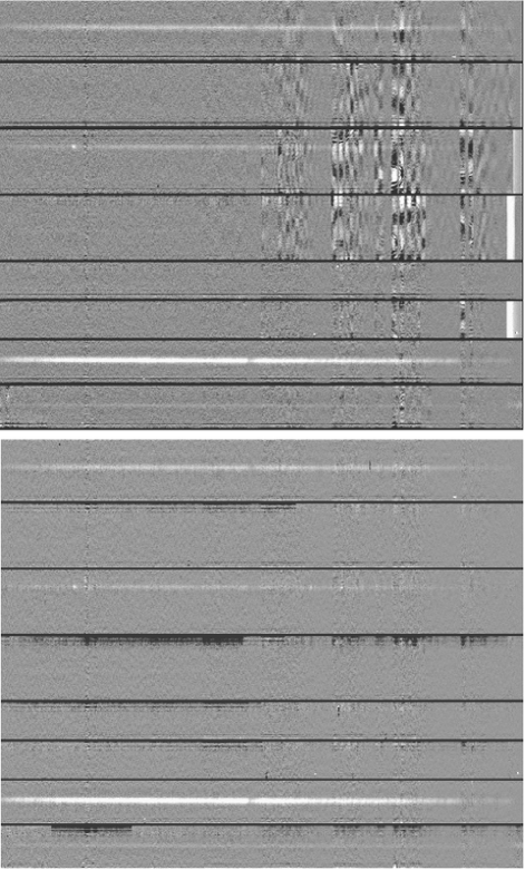
Figure 2: Example of the efficiency of the fringing subtraction procedure. The top half of the figure shows the result of combining 10 jittered VVDS exposures without the subtraction of the fringing residuals. The bottom half shows the result of combining the same 10 exposures with the subtraction. Only a small portion of the entire CCD frame is shown.

The accuracy of the wavelength calibration changes slightly from grism to grism, but the rms residuals around the best fitting relation typically amount to one fifth of a pixel. For the VVDS data, obtained with the Low Resolution Red VIMOS grism, which produces spectra with a linear dispersion of 7.14 Å/pixel, a fit with a third degree polynomial results in a wavelength calibration with a median rms residual of 1.005 Å. Figure 1 shows the distribution of rms residuals for a total of 16,936 slits: although the distribution shows the presence of a tail extending to high rms residual values, only approximately 0.9 percent of the slits show a wavelength calibration with rms residuals larger than 3.0 Å. Contrary to the case of spectra location, for wavelength calibration the local instrument model always provides the most accurate calibration information, and therefore it is the one used in the reduction of scientific observations. Using VIPGI data browsing and plotting tools it is possible to carry out an accurate visual check of the quality of the wavelength calibration, and also re-compute such calibration for individual slits or fibers, after having eliminated from the list of spectral lines significantly deviant ones.

The accuracy and stability of the wavelength calibration are obviously of the greatest importance for a spectroscopic survey like the VVDS. However the accuracy with which the Inverse Dispersion Solution maps the true wavelength calibration of VIMOS observations cannot be quantified solely on the basis of the rms residual values obtained in the calibration procedure. In fact changes in temperature or flexures within the instrument might significantly alter this mapping between the times when the science and the calibration exposures are taken (calibration lamp exposures are typically taken only at the end of a sequence of exposures, and sometimes during the following day). Therefore it is important to re-consider the issue of the wavelength calibration accuracy on the basis of the reduced science data and redshift measurements, and we do that in Section 5.

4 Science data reduction

The first step in the reduction of VIMOS science data is the canonical preliminary reduction of CCD frames, which includes prescan level and average bias frame subtraction, trimming of the frame to eliminate pre and overscan areas, interpolation to remove bad CCD pixels, and flat fielding. For VVDS data, taken with the Low Resolution Red VIMOS grism, the flat fielding of the data is not carried out, since flat field exposures, obtained using an internal halogen lamp which illuminates the reflective cover of the telescope Nasmyth focus shutter screen, show the presence of a significant amount of fringing. The spatial frequency of this fringing pattern is too high to be reliably removed with some surface fitting procedure, and the pattern present in flat field exposures results completely different from the one present in science exposures, due to the different spectral energy distribution of the halogen lamp and of the night sky. As the noise introduced by flat fielding VVDS data with such fringing-rich flat field frames is actually larger and more structured than that produced by the CCD pixel to pixel sensitivity variations, it was decided to eliminate the flat fielding altogether from the VVDS data reduction scheme.

After the preliminary reduction step, subsequent data reduction steps are carried out on all MOS slits individually, one slit at a time. Since VIMOS is known to suffer from the presence of some flexures within the instrument, the first among such steps is a refinement of the wavelength calibration. This operation is carried out using a number of skylines, by comparing their known wavelength with the one derived using the local model Inversion Dispersion Solution for the given slit. If any discrepancy is measured, an offset is introduced into the Inverse Dispersion Solution to compensate it. In practice this is a virtual offset to be applied to all pixel coordinates of a given slit or fiber spectrum at the moment of its extraction, discussed here below.

The following steps in the data reduction procedure include object detection and sky subtraction from each MOS slit spectrum. The object detection procedure is based purely on the data themselves, and does not use any prior information from the MOS mask design procedure to locate object spectra within the data. The raw data slit spectrum is collapsed over a user-defined wavelength interval, following the geometrical shape defined by the Curvature Model for the given slit, to produce a slit cross-dispersion profile. A robust determination of the average signal level and its rms variations in this profile is obtained using an iterative sigma-clipping procedure, and objects are detected as groups of contiguous pixels all above a given detection threshold, expressed in units of the signal level rms variations. For VVDS data we use a detection threshold of $2\sigma$, and a minimum object size of 3 pixels. Possible spurious detections, often taking place close to the slit edges, are removed at a later stage, during the visual inspection of the extracted spectra. All sections of the slit cross-dispersion profile devoid of objects are considered sky regions, and are used in the original raw data slit spectrum to derive a median estimate of the sky spectrum, which is then subtracted from the whole slit data.

Figure 3: Block diagram summarizing the main steps involved in the reduction of MOS data using VIPGI.

The sky-subtracted slit spectra are then two-dimensionally extracted using the tracing provided by the slit Curvature Model, and resampled to a common linear wavelength scale. Only after this point the single exposures of a jitter sequence are combined together. The main reason to use a jitter sequence for the VVDS observations is to help eliminate the strong fringing pattern present in VIMOS observations obtained with the Low Resolution Red grism. All VVDS observations are obtained using a 5 offsets pattern, with offsets of 0.75 arcsec between exposures. For each slit, the two-dimensionally extracted spectra from all exposures are median-combined a first time without taking into account the jitter offsets, to produce a sky-subtraction and fringing pattern residual map. Since the jitter offsets are somewhat smaller that the typical object size, the median combination is not enough to eliminate completely the object spectrum from these residual maps, and therefore the object spectra areas are masked out from the single slit spectra before the combination, interpolating across adjacent sky-only parts of the spectrum. The residual map is then subtracted from all single exposure spectra. At this point a second combination is carried out, this time taking into account the jitter offsets. The combination procedure uses the measured object positions derived at the object detection stage to derive a very accurate determination of the telescope offsets applied through the jitter sequence. The single exposure residual-map-subtracted spectra are offsetted to compensate for the effect of the jitter, and a final average two-dimensional spectrum for each slit is obtained. Figure 2 shows two examples of such two-dimensional spectra, as obtained with and without the subtraction of the residuals map, to illustrate the effectiveness with which the adopted procedure removes the fringing pattern from the data. This removal is most efficient when only a faint object spectrum is present in the slit, as in this case the adopted jitter pattern allows to remove without problems the object spectrum from the no-offset combination of the jittered exposures. As the objects get brighter and larger their extended spectra can prevent a reasonable estimate of the residual pattern to be obtained, and therfore the removal of the fringing residuals becomes less accurate.

The object detection process is repeated on the combined spectra, to produce the final catalog of detected spectra, and a one-dimensional spectrum is extracted for each detected object using Horne optimal extraction procedure (Horne, 1986). Finally spectra are flux calibrated, using a simple polynomial fit to the instrument response curve, derived from observations of spectrophotometric standard stars, and corrected for telluric absorption features. The last correction is based on a template absorption spectrum derived for each combined jitter sequence from the data themselves. Figure 3 shows a block diagram summary of the various steps involved in the reduction of a MOS observation with VIPGI.

5 The quality of spectra extraction and wavelength calibration

One rather obvious criterion we have used to assess the quality of our data reduction pipeline is to compare its results with those obtained via a purely manual data reduction carried out using IRAF. Unfortunately the time requirements for a manual IRAF reduction are rather expensive, and this comparison could be carried out only for a few tens of spectra. It has shown nonetheless that the quality of VIPGI-reduced spectra, in terms of continuum shape and signal to noise ratio at all wavelengths, is basically the same of the one obtained with a manual IRAF reduction.

Figure 4: Comparison between the R-band magnitudes from the photometric VVDS catalog and the magnitudes computed integrating the observed spectrum with the equivalent filter response curve. The top panel shows the full distribution of data points, while the bottom panel shows mean and $1\sigma\ rms$ scatter in half magnitude bins.

More systematically, we have compared the R and I-band magnitudes from the photometric catalog used to build the VVDS sample with the magnitude derived integrating the flux in the observed spectrum with the appropriate filter response curve. The results of such a comparison are shown in Figure 5 of LeFèvre et al. (2004) for the I-band magnitudes, and in Figure 4 for the R-band ones. We can say there is a satisfactory agreement between the spectral fluxes and the photometric magnitudes, although a significant scatter can be seen in this comparison. Most of this scatter is certainly due to the flux calibration procedure adopted for the VVDS. In practice we are not trying to obtain a nightly flux calibration, but we are using only a generic calibration template to reproduce the correct spectral energy distribution shape, without any specific attempt to obtain the right absolute flux normalization. Thus variations in the sky transparency or in seeing conditions are not taken into account by our flux calibration procedure, and show up in the scatter visible in the figure.

The most important quality checks on VVDS data are the one about wavelength calibration, and the accuracy and stability of redshift measurements we can obtain with VVDS data reduced with VIPGI. As discussed already in section 3.2, the accuracy of the wavelength calibration relation measured on the lamp exposures does not provide a complete picture of the global calibration accuracy for VIMOS data. We are therefore using the reduced spectra themselves to assess this quality.

Figure 5: The distribution of differences in redshift measurements from repeated VVDS observations of a set of 150 objects.

Using redshift measurements we can test the absolute stability of the wavelength calibration, and this test can be carried out in two different ways: within VIPGI, by comparing repeated observations of the same objects, and via an external comparison, by comparing VIMOS VVDS observations reduced with VIPGI with FORS2 observations obtained by the K20 and GOODS surveys in the CDFS. As we are interested in measuring the stability of the wavelength calibration, and not the overall reliability of the redshift measurement process, we use in this comparison only those spectra for which the separate redshift measurements are in agreement (within a z interval of 0.1). We have 150 repeated observations among the VVDS data which produce redshift measurements in agreement between them: the differences have an average value of 0.0003, with an rms scatter of 0.0010; the distribution of these differences is shown in Figure 5. We also have 41 and 27 galaxies in common with the K20 and GOODS survey, with redshift measurements in agreement. The differences have an average value of -0.0004 and -0.0006, with an rms scatter of 0.0018 and 0.0013, respectively. The global distribution of these differences is shown in Figure 6. Keeping into account the uncertainties that are contributed to the redshift measurements by the cross-correlation or line location procedures themselves, these measured uncertainties in the redshift determinations allow us to say that the absolute stability of the wavelength calibration in the VVDS data reduced with VIPGI is at the level of 2 to 3 Angstrom, significantly less than the linear dispersion coefficient for these spectra (7.14 Å/pixel).

Figure 6: The distribution of differences in redshift measurements from a comparison between VVDS and K20 or GOODS observations.

One final measure of the quality of the spectra extraction process is the fraction of failures in this process. There are many possible sources for these failures, going from spurious detections in the parent photometric catalog that result in no object being present in the slits, or errors in the astrometric calibration of the catalog resulting into a poor centering of the object in the slits, to slits vignetted by the telescope guide camera probe, to problems in the sky subtraction within a slit resulting into a failure in detecting a real object spectrum, and to spectra characterized by an almost absent continuum coupled with relatively strong emission lines that escape detection. Overall, for the VVDS observations and the 16,936 slits reduced thus far the total fraction of failures is approximately 3.9%. Eliminating the cases where this failure is not due to the data reduction software we can estimate that on average, if we exclude pure emission line spectra objects, VIPGI is succesfully extracting a spectrum for 98 % of the slits where a real spectrum is present.

6 Data Organization

As already discussed in Section 2, an automatic reduction pipeline is not enough to guarantee a quick and timely data reduction process for VIMOS data. An efficient organization of the data and easy procedures for data browsing, to be used while assessing the quality of the various data reduction steps, are two components as important as the speed of the pipeline for the global data reduction process. It is mainly for this reason that VIPGI provides its own, VIMOS specific, data organizer.

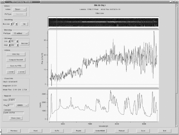
Figure 7: The ”slit summary plot”, showing the 2-dimensional and 1-dimensional spectra for one VVDS object, and the sky spectrum for the same slit.

VIMOS data are archived following standard ESO-VLT naming schemes, and therefore the astronomer gets a set of FITS files named something like VIMOS-2003-10-12T22:45:54.123.fits, names that do not convey any information about the nature of the file they represent. Moreover VIMOS observations typically result in a lot of files being produced, at least four times those produced by a typical single CCD instruments. To facilitate as much as possible the data reduction process it was decided to build VIPGI around an automatic data organizer that takes care of organizing the data in such a way as to make mistakes while selecting input files for the various reduction steps very unlikely to happen.

The first operation required in using VIPGI to reduce VIMOS data is to import the data within the VIPGI data organizer structure; the raw VIMOS data are copied from their location (a DVD from ESO archive or a directory on the astronomer’s computer disk) into a pre-defined directory tree, divided by instrument mode (MOS, IFU, or Imaging) and by quadrant. Furthermore, they are also logically divided into separate Data Categories and Types: a separate category for each MOS mask, with arc lamp, flat field, and science exposures as separate types; a separate category for each IFU target, plus one for arc lamps, and one for flat field frames. Files are also renamed with a naming scheme that reflects the logical categories used to group the data. As a result, it is very simple to define an homogeneous data-set to be used as the input for any given data reduction recipe. As part of the import operations, auxiliary calibration tables needed by the pipeline recipes are also appended to the FITS files: the “CCD table”, containing informations about CCDs bad pixels; the “GRISM table”, containing data about the spectra produced by the grism used for the observation (length of the raw spectra, wavelength interval over which to extract the 1-dimensional spectra, and over which to carry out object detection before extraction); the “LINE CATALOG table”, containing wavelengths of arc lamp lines (or sky lines in case one is using them for wavelength calibration); the “Spectrophotometric table”, containing the flux measurements for a spectrophotometric standard star. The data organizer process automatically appends to each file, according to its type, the suitable tables.

7 Spectra Plotting and Analysis

A number of different possibilities exist for browsing through one-dimensionally and two-dimensionally extracted spectra. The simplest one is to display the reduced FITS file with an image display tool like skycat, capable of handling in a simple way the display of FITS image extensions. In this way it is possible to browse quickly through all stages of the data reduction process, as all the important intermediate reduction products are appended as image or table extensions to the output FITS file.
Besides the simple image display, ad-hoc display and plotting functions have also been developed. Two-dimensional slit spectra for a MOS jitter sequence can be plotted together with all the single-exposures 2D spectra used for the combination, to check the reality of spectral features and the quality of fringing and sky residuals removal.

A tool for plotting and analyzing the extracted one-dimensional spectra is also provided. This tool allows the astronomer to plot each one of the one-dimensional spectra, together with the corresponding two-dimensional and sky 1D spectra. In this way it is possible to visually check the reality of spectral features that are present in the one-dimensional spectrum, which could be due to sky, zero order or fringing subtraction residuals. It is also possible to zoom in and out all three spectra, to edit the one-dimensional spectrum, smooth it with a simple square window function, measure the signal to noise over a selected wavelength interval, and fit the position of a selected spectral line. The astronomer can also obtain quick redshift estimates by fitting or marking the position of a set of spectral lines, and using a function that will compute a list of possible redshifts based on a list of known emission and absorption lines in galaxy spectra. Once the user has chosen one possible solution, the expected positions of all the lines in the list are marked on the plot, to visually inspect the goodness of the redshift determination.

A “summary” plotting tool is also provided (see Figure 7), which incorporates in one display window the functionality of the one-dimensional spectrum, of the lambda calibration, and of the cross-dispersion slit profile plotting tools. All functionalities from the one-dimensional plotting tool are preserved. In addition, it is also possible to display information on the astronomical object whose spectrum is being plotted.

8 Summary

We have developed VIPGI, a new tool designed to organize, reduce and analyze data obtained with VIMOS, the imaging spectrograph built by the VIRMOS Consortium for the European Southern Observatory. This tool is being used to handle all the spectroscopic data obtained for the VIMOS VLT Deep Survey, aiming to measure 150,000 galaxy redshifts.

VIPGI provides powerful data organizing capabilities, a small set of data reduction recipes and dedicated data browsing and plotting tools to check on the results of all critical data reduction steps, and to plot and analyze final extracted 1D and 2D spectra.

We have performed many data quality check demonstrating that VIPGI can be used to achieve a data reduction accuracy comparable to the one obtained using standard IRAF tasks. Moreover, its high reduction speed makes our pipeline the only reasonable tool to be used to reduce the high amount of data that a modern instrument such as VIMOS produces.

VIPGI has been extensively used while reducing more than 20,000 spectra for the VIMOS VLT Deep Survey and it is now being used routinely to reduce all kinds of VIMOS data in the VIMOS Data Reduction Support Centers in Milano and Marseille.

References

- Bottini et al. (2004) Bottini, D., et al. 2004 A&A, submitted
- Colless et al (1990) Colless, M., Ellis, R. S., Taylor, K., Hook, R. N., 1990, MNRAS, 244, 408
- Colless et al. (2001) Colless, M., Dalton, G., Maddox, S., et al., 2001, MNRAS, 328, 1039
- Horne (1986) Horne, K., 1986, PASP, 98, 609
- [Le Fèvre et al. (1995) Le Fèvre, O., Crampton, D., Lilly, S. J., Hammer, F., Tresse, L., 1995, ApJ, 455, 60
- Le Fèvre et al. (2000) Le Fèvre, O., et al. 2000, SPIE, 4008, 546
- Le Fèvre et al. (2002) Le Fèvre, O., et al. 2002, The Messenger, 109, 21
- Le Fèvre et al. (2004) Le Fèvre, O., et al. 2004, A&A, submitted
- (9) Paioro, L., Garilli, B., Scodeggio, M., Franzetti, P., 2004, astro-ph/0406117
- (10) Scodeggio, M., Zanichelli, A., Garilli, B., Le Fèvre, O., Vettolani, G., 2000, A.S.P. Conference Series, 283, 451
- Strauss et al. (2002) Strauss, M. A., Weinberg, D. H., Lupton, R. H., et al., 2002, AJ, 124, 1810
- Zanichelli et al. (2004) Zanichelli, A., et al. 2004, A&A, submitted