The Lifetimes and Evolution of Molecular Cloud Cores

Abstract

We discuss the lifetimes and evolution of clumps and cores formed as turbulent density fluctuations in nearly isothermal molecular clouds. In order to maintain a broad perspective, we consider both the magnetic and non-magnetic cases. In the latter, we argue that clumps are unlikely to reach a hydrostatic state if molecular clouds can in general be described as single-phase media with an effective polytropic exponent $\gamma_{\rm e}<4/3$. In this case, clumps are expected to be short-lived, either proceeding directly to collapse, or else “rebounding” towards the mean pressure and density as the parent cloud. Rebounding clumps are delayed in their re-expansion by their self-gravity. From a simple Virial Theorem calculation, we find re-expansion times $\sim 1$ Myr, i.e., of the order of a few local free-fall times $t_{\rm fc}\equiv L_{\rm J,c}/c$, where $L_{\rm J,c}=\sqrt{\pi c^{2}/G\rho_{\rm c}}$ is the Jeans length at the clump’s mean density $\rho_{\rm c}$ and $c$ is the isothermal sound speed.

In the magnetic case, we present a series of driven-turbulence, ideal-MHD numerical simulations in which we follow the evolution of clumps and cores in relation to the magnetic criticality of their “parent clouds” (the numerical boxes). In subcritical boxes, magnetostatic clumps do not form. A minority of moderately-gravitationally bound clumps form which however are dispersed by the turbulence in $\lesssim 1.3$ Myr. An estimate of the ambipolar diffusion (AD) time scale at the physical conditions of these cores gives characteristic times $\gtrsim 1.3$ Myr, suggesting that these few longer-lived cores can marginally be “captured” by AD to increase their mass-to-flux ratio and eventually collapse, although on time scales not significantly longer than the dynamical ones. In supercritical boxes, some cores manage to become locally supercritical and collapse in typical time scales of 2 $t_{\rm fc}$ ($\sim$ 1 Myr). In the most supercritical simulation, a few longer-lived cores are observed, which last for up to $\sim 3$ Myr, but these end up re-expanding rather than collapsing, because they are sub-Jeans in spite of being super-critical. Fewer clumps and cores form in these simulations than in their non-magnetic counterpart.

Our results suggest that a) Not all cores observed in molecular clouds will necessarily form stars, and that a class of “failed cores” should exist, which will eventually re-disperse, and which may be related to the observed starless cores. b) Cores may be out-of-equilibrium, transient structures, rather than quasi-magnetostatic configurations. c) The magnetic field may help reduce the star formation efficiency by reducing the probability of core formation, rather than by significantly delaying the collapse of individual cores.

1 Introduction

One of the most important goals in the study of star formation is to understand the state and physical conditions of the molecular cloud cores from which the stars form. The prevailing view (which we hereafter refer to as the “standard (magnetic support) model” of star formation; e.g., Mouschovias 1976a,b; Shu, Adams & Lizano 1987) is that low-mass star-forming clumps evolve into dense cores along a sequence of quasi-magnetostatic states as magnetic support is lost by ambipolar diffusion. This process has a relatively long characteristic time scale, typically estimated to be significantly larger than the local clump free-fall time (e.g., Shu et al. 1987; McKee et al. 1993). During this time, the contracting clump is supported against its self-gravity by the magnetic field in the direction perpendicular to it, and by a combination of thermal and micro-turbulent pressures along the field (e.g., Lizano & Shu 1989; McLaughlin & Pudritz 1996).

The support from magnetic fields is included through the consideration of the mass-to-magnetic flux ratio of the core. For isolated or periodic structures, in which mass cannot be accreted from the surroundings, and under ideal MHD conditions, the magnetic flux is conserved, and therefore so is the mass-to-flux ratio (Chandrasekhar & Fermi 1953; Mestel & Spitzer 1956). Thus, self-gravity cannot overcome the magnetic support if the mass-to-flux ratio is smaller than some critical value, and collapse can only occur as the neutrals in the gas slowly slip across field lines by ambipolar diffusion (see, e.g., Mestel & Spitzer 1956; Mouschovias & Spitzer 1976; see also the reviews by Shu et al. 1987 and McKee et al. 1993).

Additionally, although in the standard model the magnetic support is fundamental, discussions of non-magnetic equilibrium configurations are very often encountered in the literature. These configurations have generally either finite or diverging central densities. The former are generally based on the so-called Bonnor-Ebert (BE; Ebert 1955; Bonnor 1956) spheres, which are solutions of the Lane-Emden equation, and can be either truncated at some finite radius, beyond which a hotter, less dense medium is assumed to confine the sphere, or infinite (“extended”). Truncated configurations have recently been taken as “templates” for comparison with observations of column density profiles in real cores (e.g., Johnstone et al. 2000; Alves, Lada & Lada 2001; Evans et al. 2001; Harvey et al. 2001), even though Shu et al. (1987, sec. 4.1) had already pointed out that such truncated structures may have little relevance to actual cores in molecular clouds because they are in contact with a large reservoir of cold gas, and that a maximum contrast of 14 contradicts the observational evidence that molecular clouds typically have H₂ densities ranging from $10^{2}$ cm^-3 (average) to well in excess of $10^{6}$ cm^-3 in cores (see, e.g. Goldsmith 1987.) Various geometries other than spherical have also been considered for non-magnetic equilibrium solutions (e.g., Curry 2000; Lombardi & Bertin 2001). Concerning structures with diverging central densities, the best known example is the singular isothermal sphere (e.g., Shu 1977).

On the other hand, it is well established that the molecular clouds within which the cores form are turbulent, with linewidths that are supersonic for scales $\gtrsim 0.05$ pc (e.g., Zuckerman & Evans 1974; Larson 1981; see also the review by Blitz 1993 and references therein), generally interpreted as magnetohydrodynamic (MHD) supersonic turbulent motions. Being supersonic (and possibly super-Alfvénic; see below), these motions in general dominate the support against the clouds’ self-gravity, with thermal pressure being dominant only at subsonic scales (Padoan 1995; Vázquez-Semadeni, Ballesteros-Paredes & Klessen 2003a). In this environment, the molecular cloud clumps and cores are in fact likely to be the turbulent density fluctuations themselves within the clouds (von Weizsäcker 1951; Bania & Lyon 1980; Scalo 1987; Elmegreen 1993; Ballesteros-Paredes, Vázquez-Semadeni & Scalo 1999;Klessen, Heitsch & Mac Low 2000; Padoan et al. 2001; Heitsch, Mac Low & Klessen 2001).

Moreover, in a turbulent environment, the density and magnetic field strength are only very poorly correlated locally, at least when gravity is not important in the formation of the density sturctures (Passot, Vázquez-Semadeni & Pouquet 1995; Padoan & Nordlund 1999; Ostriker, Stone & Gammie 2001; Kim, Balsara & Mac Low 2001; Passot & Vázquez-Semadeni 2003). Thus, the clumps and cores can in principle be formed with a distribution of mass-to-flux ratios. For ideal isolated or periodic configurations, this distribution is bounded from above by the mass-to-flux ratio of the parent cloud (cf. §3.3) for as long as ambipolar diffusion is negligible (i.e., at densities $\lesssim 10^{4}$ cm^-3). Real molecular clouds are not isolated nor periodic, and can accrete mass along the magnetic field to eventually become supercritical (Hartmann, Ballesteros-Paredes & Bergin 2001), although this is likely to occur on time scales much longer than those of core evolution. So, for the purpose of studying core evolution, the mass-to-flux ratio of the parent cloud can be considered constant.

Within this framework, if the parent cloud is subcritical, then in principle supercritical cores can only form through the action of ambipolar diffusion, in agreement with the scenario of the standard model. Indeed, numerical simulations of supersonic turbulence in subcritical boxes without ambipolar diffusion have shown that collapse does not occur (Ostriker, Gammie & Stone 1999; Heitsch et al. 2001). On the other hand, if the parent cloud is supercritical, then in principle both sub- and supercritical substructures can form, even under ideal MHD. The latter can collapse if they are also gravitationally unstable with respect to the thermal pressure, a case we will sometimes refer to as “super-Jeans”.

Observationally, several recent studies (e.g., Crutcher 1999, 2004; Bourke et al. 2001; Crutcher, Heiles & Troland 2002) suggest that molecular clouds are the objects with highest mass-to-flux ratios (within the uncertainties) in the hierarchy going from diffuse medium to molecular cloud cores. Furthermore, Nakano (1998) has suggested that the large observed column densities of cores are difficult to reconcile with the relatively low column density enhancements expected for subcritical cores with respect to their parent clouds, while Padoan and coworkers (e.g., Padoan & Nordlund 1999; Padoan at al. 1999; Padoan, Goodman & Juvela 2003) have performed several synthetic observations of cores in simulations of MHD turbulence suggesting that molecular clouds are super-Alfvénic. Finally, like their parent molecular clouds, the clumps and cores (density peaks) within them are not isolated, but are connected to their surrondings, and so their masses are not fixed, especially in a turbulent environment. The non-isolated nature of the cores has been taken into account within the standard model (e.g., Lizano & Shu 1989; Curry 2000), but still under the assumption of a quasi-static evolution.

There thus appears to exist a conceptual gap between the standard assumption of quasi-hydrostatic clump/core evolution and the turbulent nature of the clouds in which they form, the natural question being whether cores formed dynamically in a turbulent medium can settle into the (magneto-)hydrostatic equilibria assumed in the standard model. Instead, they might as well be either pushed directly into collapse, or re-expand and merge back with their environment. Recently, Li & Nakamura (2004) have addressed this issue by considering the formation of dense cores in two-dimensional simulations of sheet-like, strongly magnetized clouds including a prescription for ambipolar diffusion. In the present paper we consider the problem from a more general point of view, by discussing clump and core formation in both strongly and weakly (including non-magnetic) magnetized clouds, investigating the lifetimes of clumps formed by transient turbulent fluctuations and the evolution of their Jeans number and magnetic criticality in relation to that of their parent molecular clouds. We begin (§2) by presenting and discussing the main assumptions that underlie our approach, as well as observational and theoretical evidence that supports them. We then proceed to give some general considerations in (§3) in both the non-magnetic and magnetic cases. With respect to the former, in §3.1 we present a qualitative discussion of the reasons why hydrostatic configurations are unlikely, in single-phase, nearly isothermal, non-magnetic turbulent flows. This implies that dynamically compressed regions must either proceed to collapse right away or re-expand. In §3.2 we then give a simple estimate of the re-expansion time for clumps that do not collapse (which we call “failed” clumps). In the magnetic case, in §3.3 we give a qualitative discussion of the formation and nature of cores in relation to the magnetic criticality of their parent cloud.

In §§4 and 5 we then present a series of three-dimensional numerical simulations aimed at studying the lifetimes of cores in non-magnetic and magnetic sub- and supercritical environments, first describing the numerical method and parameters (§4.1), resolution considerations (§4.2) and core analysis procedure (§4.3), and then the results (§5). Finally, in §6 we discuss some implications and caveats of our results, and in §7 we give a summary and concluding remarks.

2 Assumptions

In this section, we describe the assumptions underlying the discussions and calculations in this paper, as well as the evidence supporting them. Nevertheless, as will be clear from the discussion, the assumptions are not conclusively proven, and therefore it must be kept in mind that our results are of course subject to the applicability of our assumptions.

2.1 Single-phase isothermal medium

Throughout this paper we assume that the gas within molecular clouds responds isothermally to compressions (i.e., that it obeys an isothermal “effective” equation of state $P=c^{2}\rho$, where $P$ is the thermal pressure, $\rho$ is the density, and $c$ is the sound speed), and that it is at the same temperature throughout the volume considered. Although this is the most common assumption for numerical simulations of molecular clouds (see, e.g., the work of Padoan, E. Ostriker, Mac Low, Klessen, Bate, Bonnell and their coworkers; see also the reviews by Vázquez-Semadeni et al. 2000; Mac Low & Klessen 2004) because molecular gas is typically at temperatures $\sim 10$–15 K, the true thermodynamic behavior of molecular gas is still an open issue.

The cores in the survey of Jijina, Myers & Adams (1999) span almost an order of magnitude in temperature, from $\sim$ 5 to 40 K, although indeed with a strong concentration between 10–15 K, and presumably owing in most cases to direct heating by nearby stellar objects, rather than to $PdV$ mechanical heating. In the absence of direct stellar/protostellar heating, the gas tends to have more uniform temperatures. Indeed, the subsample of cores with no embedded clusters of Jijina et al. has a narrower temperature distribution, while a study of the dark cloud TMC-1 by Pratap et al. (1997) gives nearly uniform temperatures, between 8 and 10 K, even though the density spans nearly an order of magnitude.

Nevertheless, precise isothermality is not expected in molecular clouds. Scalo et al. (1998) summarized results on the likely values of the exponent $\gamma_{\rm e}$ that appears in polytropic equations of state of the form $P\propto\rho^{\gamma_{\rm e}}$ (see also Myers 1978; Larson 1985). For molecular gas, Scalo et al. found $1/3\lesssim\gamma_{\rm e}\lesssim 1$ for $10^{3}~{}{\rm cm}^{-3}\lesssim n\lesssim 10^{5}~{}{\rm cm}^{-3}$ in the absence of embedded protostellar sources. Recent calculations of the effective polytropic index by Spaans & Silk (2000) find a similar range for present-day Galactic molecular gas. More recently, Li, Klessen & Mac Low (2003) have investigated the dependence of the fragmentation process fragmentation on the value of the polytropic exponent in molecular clouds.

For the purposes of the present paper, the most important thermodynamic consequences of assuming isothermality (i.e., $\gamma_{\rm e}=1$) are that the increase in thermal pressure during gravitational collapse cannot eventually halt it (something which would require $\gamma_{\rm e}>4/3$ for spherically-symmetric collapse; e.g., Hayashi 1967; Larson 1969; Low & Lynden-Bell 1976; Masunaga & Inutsuka 1999; see also the discussion in §3.1), and that the medium consists of a single thermodynamic phase. A two-phase, or “thermally bistable”, nature would require the existence of an intermediate thermally unstable density range with $\gamma_{\rm e}<0$ between density ranges with $\gamma_{\rm e}>0$ (e.g., Field, Goldsmith & Habing 1969). However, we see that the $\gamma_{\rm e}$-range estimated by Scalo et al. (1998) and Spaans & Silk (2000) for the densities of interest, $1/3\lesssim\gamma_{\rm e}\lesssim 1$, is completely contained within the interval $0<\gamma_{\rm e}<4/3$, and therefore also does not allow for neither of those two phenomena. Thus, in this sense, our isothermal assumption is consistent with those $\gamma_{\rm e}$-range estimates.

However, we must point out that Gilden (1984) has suggested that a thermally unstable range with $\gamma_{\rm e}<0$ may exist in molecular gas, and, in consequence, allow for the possibility of thermal bi-stability. If this does indeed occur, then our discussion of the impossibility of producing Bonnor-Ebert-type hydrostatic structures in §3.1, based on the non-availability of a hotter, more tenuous confining medium, is invalidated. Moreover, Blitz & Williams (1999) have argued that the HI gas may pervade the volume within clumps, by showing an anticorrelation between the CO and the HI emission. This could also provide a confining medium for BE-type structures. Ultimately, observations and detailed studies of the heating/cooling processes in the gas should determine the goodness of the isothermal assumtion for molecular gas.

Other relatively minor consequences of using an isothermal prescription are that sound waves cannot steepen into shocks, and that the production of vorticity through the baroclininc term is inhibited. The latter limitation extends to polytropic prescriptions in general (see, e.g., Vázquez-Semadeni et al. 1996). This suggests that forthcoming improved molecular cloud simulations should solve the internal energy equation, with reasonably realistic prescriptions for the cooling and heating processes within them, as has been done for simulations of the global ISM (see, e.g., the review by Vázquez-Semadeni 2002).

2.2 Driven turbulence regime

Another assumption underlying our work in this paper is that the turbulence in molecular clouds is driven, rather than decaying, as we have used almost exclusively simulations of driven turbulence. Observationally, this is motivated by the fact that turbulence is ubiquitous in molecular clouds (e.g., Larson 1981; Blitz 1993; Heyer & Brunt 2004), including starless ones such as the so-called Maddalena’s cloud (Maddalena & Thaddeus 1985). This suggests a universal origin and maintenance mechanism for the clouds’ turbulence (Heyer & Brunt 2004). It has been suggested that the turbulence in the clouds may arise from the very accumulation mechanism that forms them out of the more diffuse atomic gas (Ballesteros-Paredes et al. 1999a; Koyama & Inutsuka 2002; Vázquez-Semadeni et al. 2003a,b; see also Hunter et al. 1986; Walder & Folini 1998; Vázquez-Semadeni 2003), through dynamical instabilities in the compressed regions. In this case, the turbulence in molecular clouds is driven for as long as the accumulation process continues, while they probably disperse afterwards, as in the recent simulations by Clark & Bonnell (2004).

In this scenario, the clouds are in fact part of the turbulent cascade from the largest scales down to the dissipative scales in the ISM, and the driving therefore occurs from the large scales. This is supported by recent comparisons between observations and either numerical simulations (Ossenkopf & Mac Low 2002) or fractional-Brownian-motion velocity fields (Brunt 2003), in which the observed fields are most consistent with the large-scale-driven turbulence numerical cases. Moreover, using Principal Component Analysis, Brunt & Heyer (2002) have estimated the spectral index of the turbulence in 23 fields of the FCRAO CO survey of the Outer Galaxy, finding that it is most consistent with the index found in numerical simulations of driven turbulence. Thus, we assume that the appropriate model for molecular clouds is that of driven turbulence, with injection at the largest scales.

In this paper we use the standard prescription of driving the flow in Fourier space. Although this allows precise control of spectral properties of the turbulence, such as the driving scale, it has the downside of injecting the energy everywhere in physical space, and is therefore not the most realistic energy injection mechanism. More realistic simulations of molecular clouds should include physical driving mechanisms, which, according to our discussion here, amount possibly to the cloud formation process itself. In any case, the driving scheme we use here should not directly interfere with the cores’ evolution, as it is applied on scales at least 10 times larger than typical core sizes. Specifically, the driving is applied at scales of 1/2 the box size, while clumps and cores in the simulations have typical sizes 0.08 and 0.04 times the box size (0.3 and 0.15 pc), respectively.

2.3 Neglect of ambipolar diffusion

The numerical simulations we present in §5 are of ideal MHD turbulence (subject only to the intrinsic numerical diffusion of the numerical scheme), and do not include ambipolar diffusion (AD). This implies that, in the case of subcritical simulations, gravitational collapse is completely suppresed. In this regard, the recent simulations by Li & Nakamura (2004) including AD, give a more accurate description of the effect of AD. On the other hand, those authors restricted their simulaions to two dimensions and did not consider the possibility of supercritical clouds, which we do here.

As a zeroth-order approximation to determining the effect of AD in our subcritical simulation, in §5.2.1 we estimate the classical AD time scale $\tau_{\rm AD}$ under the conditions of the clumps that form there, which can then be compared to the clumps’ lifetimes. If $\tau_{\rm AD}$ is much larger than the latter, then AD is not expected to have time to act during the cores’ duration. If it is comparable or smaller, then it can “capture” a transient, subcritical core, and increase its mass-to-flux ratio, eventually causing its becoming supercritical and collapse, although on time scales comparable to the dynamical lifetimes of the clumps we find in the simulations, thus not significantly delaying the collapse time.

3 General Considerations

3.1 The non-magnetic case

In this section we suggest that the formation of hydrostatic configurations is unlikely in single-phase, nearly isothermal (or, more generally, with $0<\gamma_{\rm e}<4/3$), non-magnetic flows. This is because, for nearly-isothermal flows, the production of significant density fluctuations requires supersonic turbulent compressions. These fluctuations are in general transient, and so the density enhancements they produce (“clumps”) must also be so, unless the latter happen to “land” near a stable (attracting, in the language of dynamical systems) hydrostatic equilibrium between self-gravity and thermal pressure (not turbulent pressure, because it is locally too highly variable for establishing a static configuration). In this case, after the external turbulent compression subsides, the core may evolve towards this equilibrium rather than towards either re-expansion or gravitational collapse.

It follows that hydrostatic cores can occur only if there exist stable equilibria. The best known such configurations in the non-magnetic, isothermal case are the well-known Bonnor-Ebert (BE) solutions of the Lane-Emden equation. However, the stability of these configurations relies on the fact that they are truncated at a finite radius from their center, being confined by a hotter, negligible-density medium. The boundary between the cold, dense medium and the hot, low-density one amounts to a transition between two stable phases (with $\gamma_{\rm e}>0$) mediated by a (non-populated) thermally unstable density range with $\gamma_{\rm e}<0$.

Of course, a hot confining medium is not necessary in general. For polytropic situations with $\gamma_{\rm e}>\gamma_{\rm c}$, where $\gamma_{\rm c}=4/3$ (Chandrasekhar 1961, §117; Yabushita 1968; McKee et al. 1993, sec. VI.C; Vázquez-Semadeni, Passot & Pouquet 1996), spherically-symmetric equilibria can be found even for a vanishing external pressure. This is why stars can be formed as stable entities from highly anisotropic, dynamic, time-dependent accretion (Hartmann et al. 2001). However, for bounded systems with $\gamma_{\rm e}<4/3$, the boundary pressures are indispensible in establishing stable equilibria. Such boundaries are, however, ruled out in single-phase media, in which no abrupt transition to a hotter, more tenuous medium at the same pressure is possible.

We must examine, then, the possibility of extended (i.e., non-truncated) stable equilibrium configurations, in which the core merges smoothly into its environment. To our knowledge, this remains an open question. The best-known extended equilibrium configuration is the singular isothermal sphere, which, however, is known to be unstable, and has been used in fact as the initial condition for gravitational collapse calculations (e.g., Shu 1977). A more realistic (though still spherical) configuration would be one with a finite central density. Such a configuration can be obtained by numerically integrating the Lane-Emden equation to arbitrarily large radii. However, this implies that it would be equivalent to a BE sphere of arbitrarily large radius, and would thus be gravitationally unstable (we thank D. Galli for suggesting this argument).

Other possibilities exist, however. Curry (2000) has found a new class of periodic equilibrium structures in cylindrical geometry, which he has proposed as candidates for the formation of cores in filamentary clouds. However, he did not give definitive results concerning the stability of these structures, and in fact concluded that full numerical simulations may be necessary to resolve the issue.

In this respect, numerical simulations of non-magnetic self-gravitating polytropic turbulence with $\gamma_{\rm e}\leq 1$ suggest that hydrostatic configurations do not form: the turbulent density fluctuations either re-expand, or proceed directly to collapse. This was first shown by Vázquez-Semadeni et al. (1996) for two-dimensional turbulent flows with $\gamma_{\rm e}\leq 0.3$, in which many generations of clumps were seen to appear and disappear in roughly their crossing time, until finally a strong enough compressive event occurred as to produce a gravitationally unstable core, which then proceeded to collapse in roughly its own free-fall time. This result has subsequently continued to be found in 3D simulations of non-magnetic, isothermal (e.g., Klessen et al. 2000) as well as polytropic (Bate, Bonnell & Bromm 2002; Li, Klessen & Mac Low 2003) turbulence, in which the formation of hydrostatic objects is in general not observed (R. Klessen, private communication) for $\gamma_{\rm e}<4/3$. The turbulent density fluctuations either re-expand or proceed directly to collapse in their own free-fall time.

Finally, it is worth noting that Clarke & Pringle (1997) have pointed out that cores cool mainly through optically thick lines, but are heated by cosmic rays, and therefore may be dynamically unstable, as velocity gradients may enhance local cooling.

3.2 Re-expansion time of “failed” compressions

The arguments above suggest that a significant fraction of the clumps and cores in molecular clouds may be headed towards re-expansion rather than collapse. This possibility is often overlooked in the literature, which has generally focused on the gravitational collapse of cores to form stars, and considers starless cores as “pre-stellar” (with a few notable exceptions; e.g., Taylor, Morata & Williams 1996). However, in the scenario advocated in this paper, a fraction of the starless cores may never actually form stars, and instead re-expand and disperse back into their parent molecular cloud, being natural candidates to correspond to at least some of the observed starless cores.

In the absence of self-gravity, one would expect that the re-expansion of a spherical core should be nearly identical to the compression that produced it, run backwards in time. However, in the self-gravitating case, the re-expansion process must occur on a longer time scale than the compression because of the retarding action of self-gravity. It is thus of interest to estimate their expected lifetimes.

A crude estimate of the re-expansion time can be given in terms of the Virial Theorem (VT), similarly to the analysis performed by Hunter (1977, sec. III.) to investigate the classes of solutions of unstable BE spheres. We extend his treatment to estimate the re-expansion time scale, although we consider the case of zero external pressure, because a) the density contrast between cores and their parent molecular clouds are large enough (up to factors $\sim 100$) that the external thermal pressure is negligible during the initial stages of the evolution with which we are concerned, and b) in our case of an extended core, with a smooth density profile, the whole profile varies in time, and therefore the pressure is also variable at any boundary that we choose to define (which, as a matter of fact, would be rather arbitrary). The full time-dependent problem is what is solved by the numerical simulations, but for the purpose of a simple estimate, here we consider the free re-expansion of a gas sphere subject exclusively to its self-gravity and internal pressure.

The VT for an isothermal spherical gas mass (“cloud”) of volume $V$ and mean density $\bar{n}$ in empty space is

$$\frac{1}{2}\ddot{I}=3Mc^{2}-\alpha GM^{2}/R,$$ (1)

where the overhead dots indicate time derivatives, $M=\int_{V}\rho dV$ is the cloud’s mass, $R$ is its radius, $\rho$ is the density, $I=\int_{V}\rho r^{2}dV$ is its moment of inertia, $c$ is the sound speed, and $\alpha$ is a factor of order unity. We can obtain an evolution equation for the cloud’s radius by replacing the radius-dependent density by its mean value in the expression for $I$, to find $I\approx MR^{2}$. Thus,

$$\frac{1}{2}\ddot{I}\approx M\left[R(t)\ddot{R}(t)+\dot{R}^{2}(t)\right].$$ (2)

From equations (1) and (2), we obtain

$$\left[R(t)\ddot{R}(t)+\dot{R}^{2}(t)\right]=3c^{2}-\alpha GM/R.$$ (3)

This equation can be integrated analytically, with solution

$$\tau= \frac{1}{\sqrt{3}}\biggl{[}\sqrt{(r_{2}-1)^{2}-(r_{1}-1)^{2}}+$$ (4)

$$\ln\left(\frac{r_{2}-1+\sqrt{(r_{2}-1)^{2}-(r_{1}-1)^{2}}}{r_{1}-1}\right)\biggr{]}$$

where $r_{1}$ and $r_{2}$ are the initial and final radii of expansion, normalized to the equilibrium radius $R_{\rm e}=\alpha GM/3c^{2}$, and $\tau=t/t_{\rm ff}$ is the time, non-dimensionalized to the free-fall time $t_{\rm ff}=R_{\rm e}/c$. A characteristic re-expansion time can be defined as the time required to double the initial radius (i.e., $r_{2}=2r_{1}$, a “2-folding” time), starting from an initial condition $r_{1}>1$. Figure 1a shows this characteristic time as a function of $r_{1}$. We see that when $r_{1}$ is very close to unity (i.e., linear perturbations from the equilibrium radius), the re-expansion time can be up to several times the free-fall time. Values of $r_{1}$ moderately larger than unity have the shortest re-expansion times, because the initial force imbalance is greater, yet the final size is still not much larger than twice the equilibrium radius. Finally, for larger initial radii (far from the equilibrium value), the re-expansion time approaches that of free expansion at the sound speed. These times are also long, but not because of a low expansion velocity, but because the distance to be traveled by the clump boundary from $r_{1}$ to $r_{2}$ increases proportionally to $r_{1}$. Figure 1b shows an crude “observer’s perspective” of the re-expansion time, giving the time the core’s density stays above 10% of the equilibrium-configuration density $\rho_{\rm e}$. This emulates the time the core would be visible to a high-density tracer sensitive to densities $>0.1\rho_{\rm e}$. This perspective clearly shows that the longest re-expansion times of an object that can be called a “core” correspond to those that come closest to equilibrium.

We conclude that the re-expansion time is at least larger than twice the free-fall time, making the probability of observing a core in this process larger by this factor than that of observing a free-falling core. This is consistent with the fact that molecular clouds are generally observed to contain more starless than star-forming cores (e.g., Taylor et al. 1996; Lee & Myers 1999; see also Evans 1999 and references therein).

A number of points are worth noting here. First, the database put together by Jijina et al. (1999), reports a larger fraction of star-forming than starless cores but, as those authors recognize in their section 7.1, their sample is not free of biases, with starless cores not being as well represented as the star-forming ones. This is due to the selection criteria used to select the cores in the surveys from which these authors put their database together. Instead, the Lee & Myers (1999) dataset was designed to be as free as possible from this bias, their cores being selected optically from the STScI Digital Sky Survey. Second, some observations, such as those of ammonia cores, may be biased towards selecting collapsing cores, if the densities they probe are very large; i.e., if they probe densities not regularly reached by non-collapsing clumps. The cores in the Jinina et al. sample, which is an ammonia-core database, have larger typical number densities ($n>10^{4}$ cm^-3) and a smaller starless fraction than those in the Lee & Myers optically-selected sample ($n\sim 7\times 10^{3}$ cm^-3). Indeed, in the simulations reported in §5, the failed clumps rarely exceed peak densities $\sim 5\times 10^{4}$ cm^-3.

3.3 The magnetic case

In the magnetic case, the classical Virial-Theorem (VT) analysis (Chandrasekhar & Fermi 1953; Spitzer 1968; Mouschovias 1976a,b; Mouschovias & Spitzer 1976; Zweibel 1990) predicts the existence of sub- and super-critical configurations (e.g., Shu et al. 1987) depending on whether the mass-to-magnetic flux ratio is below or above a critical value $(M/\phi)_{\rm c}$. Subcritical configurations are known not to be able to collapse gravitationally unless the magnetic flux is lost by some process such as ambipolar diffusion. Supercritical configurations, on the other hand, are analogous to the non-magnetic case, except for the fact that the cloud behaves as if having an “effective” mass, reduced by an amount equal to the critical mass (which depends on the magnetic field strength) (e.g., Spitzer 1968, §11.3.b).

A magnetized clump or core (we generically use the term “core” in this section) may thus be characterized by two nondimensional numbers, the first one being its Jeans number ($J_{\rm c}\equiv l/L_{\rm{J,c}}$), where $l$ is the characteristic core size and $L_{\rm{J,c}}$ is the Jeans length at the mean core density, measuring whether the core is gravitationally unstable with respect to the thermal support ($J_{\rm c}>1$, or “super-Jeans”) or not. The other is the core’s mass-to-magnetic-flux ratio expressed in units of the critical value for collapse, $\mu_{\rm c}\equiv(M/\phi)/(M/\phi)_{\rm cr}$. Collapsing cores must have $J_{\rm c}>1$ and $\mu_{\rm c}>1$, while cores with $J_{\rm c}>1$ and $\mu_{\rm c}<1$ can become gravitationally bound but remain in a stable magnetostatic state (under ideal MHD conditions). Finally, cores with $J_{\rm c}<1$ are Jeans-stable, and must re-expand after a transient turbulent compression, regardless of their value of $\mu_{\rm c}$. Note that both $J_{\rm c}$ and $\mu_{\rm c}$ are in general time-dependent, and also depend on the definition of the core’s boundary. A fundamental question is then what kind of cores are produced in turbulent clouds as a function of the turbulent parameters and of the cloud’s own sub- or supercritical nature.

In order to obtain insight on this, it is instructive to consider the formation of cores starting from idealized, initially uniform-density clouds, truncated at a certain size, so that the cloud’s mass-to-flux ratio is well defined. This represents also the periodic-boundary boxes of the numerical simulations. In reality, clouds are embedded in the diffuse atomic medium, and in principle there is always a large enough mass reservoir for them to be supercritical (e.g., Hartmann et al. 2001), but if the region size that needs to be considered is very large, then the time scale for accumulating this material in the molecular region is long, during which the cloud can be considered subcritical over the evolutionary time scales of individual clumps within it. We thus consider both sub and supercritical uniform initial conditions, under ideal MHD, and a fixed global mass-to-flux ratio.

In ideal MHD, it is clear that an initially subcritical core can become supercritical only if its parent cloud is supercritical. Indeed, the mass-to-flux ratio of an isolated cloud or core is independent of its radius, because both the mass and the flux are conserved quantities in this case. So, even if the whole cloud were to be compressed by a turbulent fluctuation, it could not increase its mass-to-flux ratio. As a consequence, a hard upper limit for the mass-to-flux ratio of a core is that of its parent cloud. Hence the need for the whole cloud to be supercritical if supercritical cores can ever arise under ideal MHD.

The above hard limit on the mass-to-flux ratio of a core can also be seen as follows. Consider a cubic cloud of size $L$ with uniform density $n_{0}$ and magnetic field $B_{0}$, and any flux tube of square cross section $l^{2}$, with $l\ll L$. Since in this case $M/\phi=N_{0}/B_{0}$, where $N_{0}=n_{0}L$ is the column density across the cubic domain, it is clear that $M/\phi$ for a flux tube is independent of its cross section, and equal to that of the whole (uniform) cloud. If all the mass in the flux tube were to end up in a single core, the core would still be limited to having the same value of $M/\phi$ as its parent, uniform cloud. If instead some fragmentation process (e.g., turbulent or gravitational) causes the formation of several cores along the flux tube, then each one of them will have a smaller value of $M/\phi$ than the parent cloud, because the sum of their masses is bounded from above by the mass of the flux tube, while the flux along the tube is constant.

On the other hand, a lower estimate of the mass-to-flux ratio of a core can be obtained by considering simply a region of volume $l^{3}$ within the same uniform cloud. In this case, the mass-to-flux ratio of this parcel (which is not properly a core, since it is at the same uniform density as the whole cloud) scales as $l/L$. So, for a core of size $l$ along the flux tube, we may expect its mass-to-flux ratio $\mu_{\rm c}$ to lie in the range $(l/L)\mu_{0}<\mu_{\rm c}<\mu_{0}$ when its density $n_{\rm c}$ lies in the range $n_{0}<n_{\rm c}<(L/l)^{3}n_{0}$, where $\mu_{0}$ and $n_{0}$ are respectively the parent cloud’s mass-to-flux ratio and mean density.

4 Numerical experiments

4.1 Method and parameters

We use a total variation diminishing (TVD) scheme for solving the isothermal MHD equations in three dimensions. TVD is a second-order-accurate upwind scheme, and its implementation for isothermal flows is described in detail by Kim et al. (1999). Here we use an extension of this code including self-gravity and a random turbulence driver. The boundary conditions in all our simulations are periodic. We solve the Poisson equation using the usual Fourier method. In order to achieve second-order accuracy in time, we implement an update step of the momentum density due to the gravitational force as in Truelove et al. (1997). For the turbulence random driver, we follow the method in Stone, Ostriker & Gammie (1998). As discussed in §2.2, we drive the turbulence at large scales, at wavenumber $k=2(2\pi/L)$, where $L$ is the one-dimensional size of the computational box. We adjust the kinetic energy input rate in order to maintain a roughly constant specified rms sonic Mach number $M_{\rm s}$.

The simulations presented in this section can be considered extensions of previous works by Pouquet, Léorat & Passot (1991), Ostriker et al. (1999), and Heitsch et al. (2001). In those studies, numerical simulations in which the entire computational domain is supercritical systematically undergo collapse, albeit somewhat more slowly than non-magnetic cases (by factors of 2–3). Moreover, Li et al. (2004) have shown that all cores arising in their supercritical simulations are supercritical by at least an order of magnitude. Only when the entire computational box is constrained to be subcritical is the collapse of both the large and the small scales prevented, giving rise to flattened structures. We extend those numerical works to study the lifetimes and criticality of the individual cores in relation to the criticality of their parent clouds. To this end, we now consider a series of simulations of Jeans-unstable numerical boxes, considering both magnetically sub- and supercritical cases. In view of our neglect of AD, AD-mediated contraction and subsequent gravitational collapse cannot occur in our simulations. However, we can investigate whether magnetostatic, subcritical cores with $J_{\rm c}>1$ and $\mu_{\rm c}<1$ (cf. §3.3) form in the simulations, that could then evolve quasi-statically under AD. This is done in §5.2.1.

The simulations are scale-free, and are characterized by three non-dimensional numbers: $M_{\rm s}=\sigma/c$ (the rms sonic Mach number, where $\sigma$ is the turbulent velocity dispersion and $c$ is the sound speed), $J\equiv L/L_{\rm J}$ (the Jeans number, giving the size of the box in units of the Jeans length $L_{\rm J}$), and $\beta\equiv P_{\rm th}/P_{\rm mag}=8\pi\rho_{0}c^{2}/B_{0}^{2}$ (the plasma beta, defined as the ratio of the thermal to the magnetic pressures, where the subindex “0” denotes mean values in the box and $c$ is the sound speed). The values of these parameters for all runs are respectively given in columns 2, 3 and 4 of Table 1, together with the run’s resolution (column 5) and suitable physical units, obtained as follows: The sound speed is assumed to be fixed, at $c=0.2$ km s^-1 (implying $T=11.4$ km s^-1). Then, a Larson-like relation of the form $M_{\rm s}=5\left(L/1{\rm pc}\right)^{1/2}$ (e.g., Larson 1981; Blitz 1993) gives the box size (column 6) as a function of $M_{\rm s}$ as

$$L=0.04M_{\rm s}^{2}~{}{\rm pc}.$$ (5)

The Jeans number and the box size give the mean number density density (column 7) as

$$n_{0}=500\left[\frac{J}{\left(L/1~{}{\rm pc}\right)}\right]^{2}{\rm cm}^{-3},$$ (6)

where we have assumed a mean molecular weight $m=2.4m_{H}$. In turn, the mean density and $\beta$ (at the above value of $c$) give the mean field strength (column 8) as

$$B_{0}=0.205\left(\frac{n_{0}}{\beta}\right)^{1/2}\mu{\rm G}.$$ (7)

The last two columns in Table 1 give the rms turbulent velocity dispersion and the mass-to-flux ratio of the simulation (in units of the critical value), $\mu=(\beta/\beta_{\rm cr})^{1/2}$, where $\beta_{\rm cr}$ is given as a function of $J$ as

$$\beta_{\rm cr}\sim 2/(\pi^{2}J^{2}).$$ (8)

This in turn is obtained assuming that the critical mass-to-flux ratio is $(M/\phi)_{\rm cr}\approx(4\pi^{2}G)^{-1/2}$ (Nakano & Nakamura 1978). Specifically, we get $\beta_{\rm cr}\approx 0.023$ for $J=3$ and $\beta_{\rm cr}\approx 0.013$ for $J=4$. We have verified numerically the critical $\beta$ value for the $J=3$ case as follows. We set up a white-noise initial velocity field with rms amplitude $10^{-4}c$ in each velocity component, and observe whether the maximum density in the simulation increases or becomes saturated in time. Indeed, the cases with $\beta\geq 0.03$ collapse in a runaway fashion, whereas the cases with $\beta\leq 0.01$ form magnetically-supported configurations, flattened along the mean field direction.

4.2 Resolution considerations

It is important to know when our results can be considered robust physical ones rather than numerical artifacts caused by insufficient resolution. A useful criterion for guaranteeing that the gravitational collapse of an object is followed adequately was given by Truelove et al. (1997). This criterion requires that the minimum Jeans length within the simulation be resolved by at least four zones. Heitsch et al. (2001) increased this requirement to six zones for the proper resolution of MHD waves, although this may be an excessive constraint, as those authors showed that the magnetic field can only prevent collapse if it is strong enough to provide magnetostatic support. Our interest just being to determine whether magnetostatically-supported structures arise, we consider that fulfillment of the 4-zone Jeans condition is sufficient. This is consistent with the results described below.

In general, the constraint of resolving the Jeans length by $N_{L_{\rm J}}$ zones limits the maximum resolvable density to

$$n_{\rm res}=\left(\frac{N_{\rm box}}{JN_{L_{\rm J}}}\right)^{2}n_{0},$$ (9)

where $N_{\rm box}$ is the number of zones per dimension in the computational box. Note that our definition of $J$ is different from that of Truelove et al. (1997). For the Jeans criterion, $N_{L_{\rm J}}=4$, so for our $J=4$ runs, this gives $n_{\rm res}=256n_{0}$. For the more stringent criterion of MHD-wave resolution, $N_{L_{\rm J}}=6$ zones, in which case $n_{\rm res}=114n_{0}$.

4.3 Core analysis procedure

In the §5.2, we describe in detail the evolution of the magnetic criticality and Jeans number of some selected cores in the simulations. Here we describe the procedure for measuring their mass-to-flux ratio $\mu_{\rm c}$ and Jeans number $J_{\rm c}$. Note that this is not a fully unambiguous task, because the medium is a continuum. Thus, the cores’ boundaries, and therefore their masses and sizes, are somewhat arbitrary. Moreover, the cores are in general part of a larger parent clump, which is also involved in the dynamics. A precise measurement of the structures’ energy balance would require to measure in principle all the terms in the virial theorem for them, including the surface terms (Ballesteros-Paredes & Vázquez-Semadeni 1997; Ballesteros-Paredes et al. 1999a; Shadmehri, Vázquez-Semadeni & Ballesteros-Paredes 2001; Tilley & Pudritz 2004). Thus, here we only measure the mass-to-flux ratio of the cores in an approximate way, as follows.

First, we define a structure (clump or core, which here we will generically refer to as “core”) as a connected region around a local density peak, in which the density is above a threshold value $n_{\rm t}$. Then, the mass of the core is computed directly from the density field as $M_{\rm c}=\int_{V_{\rm c}}\rho dV$, where $V_{\rm c}$ is the core volume. To compute the magnetic flux within the core, we need in principle to first compute the (vector) average of the magnetic field ($\langle{\bf B}\rangle$) within the core’s volume, and then define a surface $S$ normal to $\langle{\bf B}\rangle$ that bisects the core, in order to compute $\phi_{\rm c}=\int_{S}{\bf B}\cdot\hat{\bf n}dA$, where $\hat{\bf n}$ is the unit vector normal to $S$. For our purposes here, we use a simpler, approximate procedure. For supercritical runs, in which the cores are not very far from round, we define the core radius as $R_{\rm c}=(3V_{\rm c}/4\pi)^{1/3}$. It is easy to show that, if instead of spherical, the core is a cylinder of volume $\pi R^{2}dz$, then an aspect ratio $a\equiv R/dz$ gives an error of a factor of $a^{1/3}$ in the above estimate of the radius. At most, the aspect ratios of the cores in our moderately supercritical run are $\lesssim 4$, and are even smaller in the strongly supercritical run. Thus, the errors in the estimate of $R$ are by factors $\lesssim 1.6$. For the subcritical run, and very flattened cores, we define the core radius as the maximum distance between the density peak and all points belonging to the core. Typical sizes for the “clumps” (defined by $n_{\rm t}=10n_{0}$) and for the “cores” (defined by $n_{\rm t}=10n_{0}$) are $\sim 0.08$ and $0.04$ times the box size ($\sim 0.32$ and 0.16 pc).

With these definitions, we finally estimate the flux through the core is $\phi_{\rm c}\approx\pi BR_{\rm c}^{2}$, where $B$ is the mean magnetic field intensity through the core. The core’s Jeans number is simply computed as $J_{\rm c}=R/L_{\rm J,c}$, where $L_{\rm J,c}=\left(\pi c^{2}/G\rho_{\rm c}\right)^{1/2}$, is the mean Jeans length in the core, and $\rho_{\rm c}$ is the mean density in the core.

5 Numerical Results

5.1 Global analysis

Figure 2 shows the evolution of the global density maximum $n_{\rm max}$ for the four simulations in Table 1 with $M_{\rm s}=10$ and $J=4$ and $\beta=0.01$, 0.1, 1 and $\infty$, respectively labeled M10J4$\beta$.01, M10J4$\beta$.1, M10J4$\beta$1 and M10J4$\beta$$\infty$. The time axis is shown both in Myr (lower axis) and in units of the global free-fall time ($t_{\rm fg}\equiv L_{\rm J}/c$, upper axis). Note that runs M10J4$\beta$.01 and M10J4$\beta$.1 are evolved for over 10 Myr. This is a long time compared to recent estimates of cloud lifetimes of a few Myr (Ballesteros-Paredes, Hartmann & Vázquez-Semadeni 1999; Hartmann et al. 2001). The long integration times are just for statistical purposes, and by no means imply that we advocate longer lifetimes.

From fig. 2 it is seen that in the subcritical ($\beta=0.01$) case, $n_{\rm max}$ is typically $\sim 40n_{0}$ and seldom exceeds $\sim 100n_{0}$. The same behavior is observed in the other subcritical runs (not shown), M10J3$\beta$.01, M8J4$\beta$.01, and M10J4$\beta$.01LR. Thus, in these simulations core-like densities ($n\gtrsim 200n_{0}\sim 10^{5}$ cm^-3) are not produced. The fact that the maximum density does not stay constant also suggests that there are no magnetostatic clumps. Note that these results cannot be attributed to numerical diffusion, whose effect would be expected to act in the opposite direction of causing artificial flux loss and possibly collapse.

In contrast, fig. 2 also shows that in the supercritical runs $n_{\rm max}$ reaches values $\sim 10^{4}n_{0}$ after roughly $1/2~{}t_{\rm fg}$, although the rise from densities $\gtrsim 100n_{0}$ to $\sim 10^{4}n_{0}$ occurs on a much shorter time scale. This corresponds to the first local collapse event, as discussed in §4.3. Finally, the non-magnetic run M10J4$\beta$$\infty$ is seen to start producing collapsed objects much earlier than the magnetic supercritical runs. Thus, both the supercritical runs and the non-magnetic ones produce the first collapsed objects on times shorter than the global free-fall time as a consequence of the production of locally gravitationally unstable objects by the turbulence. However, it is seen that the effect of the turbulent compressions is diminished by the presence of the magnetic field even in the strongly supercritical case in comparison to the non-magnetic one.

5.2 Evolution of core properties

5.2.1 Subcritical case

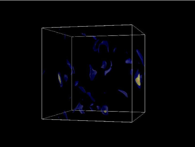
Figure 3: Animation of the density field for the subcritical run M10J4$\beta$.01, showing transparent density iso-surfaces at $n=10n_{0}$ (blue), $n=30n_{0}$ (yellow), and $n=100n_{0}$ (red). The figure shown in the paper edition corresponds to frame 223, at which the moderately-long-lived core attains its time-wise maximum central density, of just over $100n_{0}$.

In fig. 3, we show an animation of the evolution of the subcritical run M10J4$\beta$.01. Depicted are three isosurfaces at densities 10 (blue), 30 (yellow) and 100 (red) times $n_{0}$. The time interval between successive frames is $\Delta t=0.002~{}t_{\rm s}$, where $t_{\rm s}=20$ Myr is the sound crossing time for the $M_{\rm s}=10$ ($L=4$ pc) boxes. In this simulation, most density peaks (“clumps”, in this case) are seen to be extremely transient in nature, with lifetimes 0.01–0.075 $t_{\rm s}$, or 0.2–1.5 Myr (some 5–30 frames), and with poorly defined identities, the clumps actually merging with other structures or simply morphing into different shapes and sizes.

In this simulation, we only observe one clump that becomes gravitationally bound and survives for a few local free-fall times. It appears near the left boundary of the box around frame 205, and moves across it to remain near the right boundary for the rest of its existence. This core maintains peak densities $n_{\rm peak}>100n_{0}=5\times 10^{4}$ cm^-3 during 7 frames, from frame 221 to 227 (0.28 Myr), and $n_{\rm peak}\gtrsim 60n_{0}$ during $\sim 28$ frames ($\sim 1.1$ Myr), from frame 210 to frame 237. Figure 4 shows the evolution of $\mu_{\rm c}$ and $J_{\rm c}$ for this clump (defined by $n_{\rm t}=40n_{0}$) from frame 210 to 240 ($t=8.4$ to 9.6 Myr). We see that it remains strongly subcritical (well below the value for the box of 0.9), but it manages to remain significantly super-Jeans for slightly over 1.2 Myr.

This clump then represents the closest our subcritical simulation gets to producing the conditions for subsequent quasi-magnetostatic evolution mediated by AD. Nevertheless, we see that this clump’s lifetime is still quite short, because it is not very strongly gravitationally bound, and the turbulence manages to tear it appart after having formed it. It is then natural to ask whether AD would have enough time, had it been included in the simulations, to allow it to become more strongly bound, and ultimately collapse, before it is dispersed again by the turbulent motions.

To answer this question, Appendix I presents a simple estimate of the classical AD time scale under the conditions of this clump. It is found that $\tau_{\rm AD}\gtrsim 1.3$ Myr, which is very close to the duration of this clump in our simulation, suggesting that AD is possibly capable of “capturing” it and helping it decouple from the external turbulence. Note, however, that this value of $\tau_{\rm AD}$ is not significantly larger than the collapse times we observe in the supercritical simulations, and thus a core that evolves on this time scale can hardly be considered quasi-static.

Another relevant question is whether such clumps would approach a magnetostatic state if the turbulence were decaying. To test this possibility, we have conducted the additional experiment of turning off the turbulent driving at frame 210, right after the clump forms. In this case, we find that indeed the clump undergoes a few bounces, but maintains its identity for at least 1.6 Myr (the duration of the integration we performed), with no sign of disruption towards the end. This suggest that, if turbulence is turned off right after it forms the clump, then the clump does evolve towards a magnetostatic state, and can easily be captured by AD, to evolve in accordance to the standard model. Presumably, other clumps might undergo the same evolution in a decaying situation, as in the simulations by Li & Nakamura 2004.

We conclude from this section that even the densest, longest-lived clumps arising in our subcritical simulation are dispersed here because the strong magnetic field does not allow them to collapse nor achieve very strong gravitational binding, and makes them susceptible of subsequent disruption by the same turbulent field. The longest clump lifetimes are marginally long enough for them to undergo AD-mediated evolution, albeit on relatively short time scales. However, such clumps could easily become magnetostatic in a decaying turbulent field. The fundamental question then becomes whether molecular clouds are continually driven or decaying (see discussion in §6).

5.2.2 Moderately supercritical case

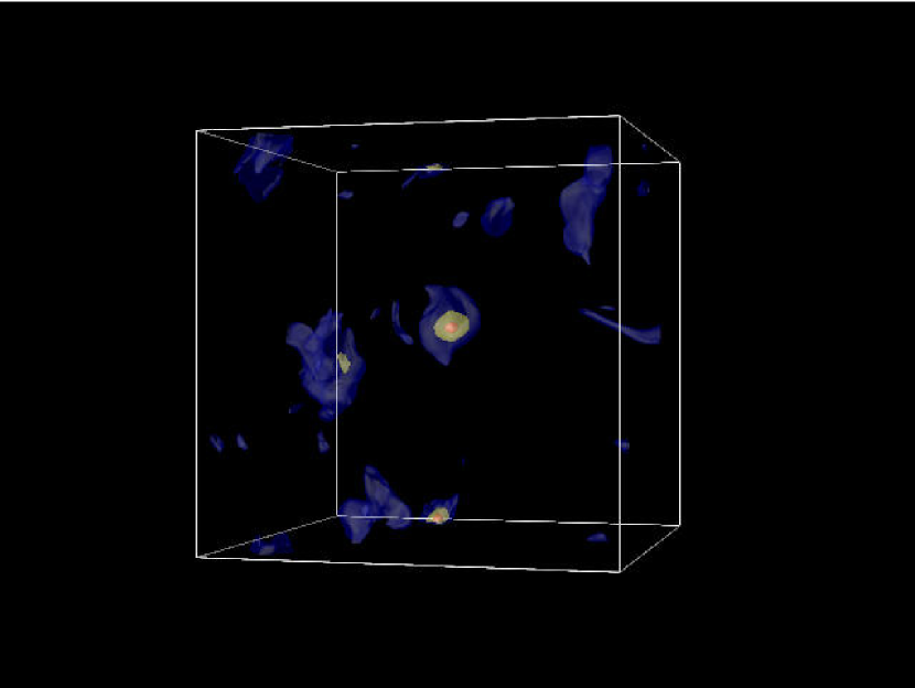
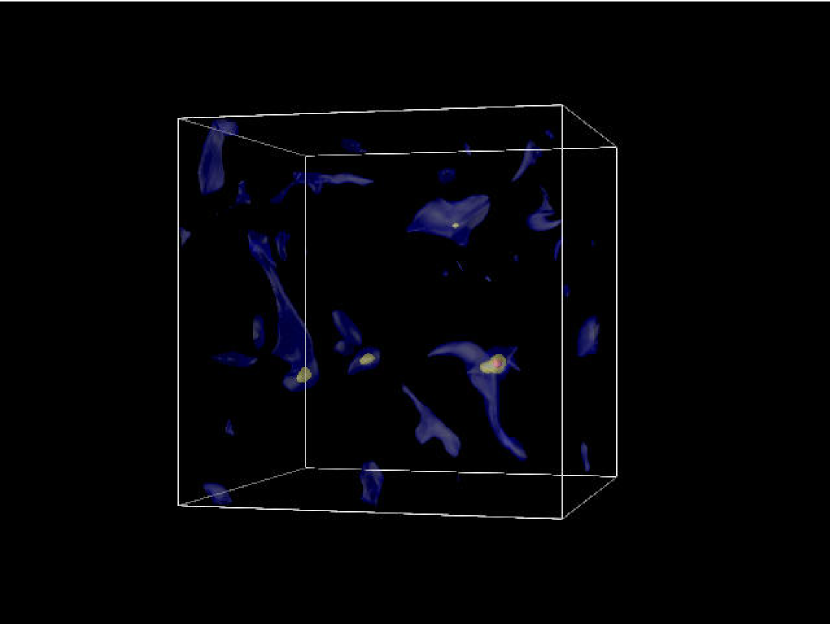
Figure 5: Animations of the supercritical runs as in fig. 3, but with the density iso-surfaces corresponding to $n=10n_{0}$ (blue), $n=100n_{0}$ (yellow), and $n=1000n_{0}$ (red). a) Run M10J4$\beta$.1. b) Run M10J4$\beta$1. The still frames in the paper edition show: (a) Frame 210 of run M10J4$\beta$.1, at which time the third (and last) collapsing core (on the left) is forming. This core is fully collapsed by frame 220. (b) Frame 55 of run M10J4$\beta$1, showing two of the long-lived but non-collapsing cores at the center (detailed in fig. 8) and left, and a collapsed core on the right.

Figure 5a shows the evolution of the moderately supercritical run M10J4$\beta$.1, again with $\Delta t=0.002~{}t_{\rm s}$, but now with the isodensity contours denoting 10 (blue), 100 (yellow) and 1000 (red) $\times n_{0}$. It is seen that in this run, objects reaching much higher peak densities, $n_{\rm peak}\gtrsim 5000n_{0}$, form since early in the evolution. Specifically, three such objects form at times $\sim 1.76$, 5.2 and 8.4 Myr (frames 44, 130 and 210, respectively). Once they have reached those densities, these objects are already collapsed, as they simultaneously have $J_{\rm c}\gg 1$ and $\mu_{\rm c}\gg 1$, and so nothing supports them against their self-gravity. In particular, they have $\mu_{\rm c}>\mu_{\rm box}$, indicating that numerical diffussion has caused magnetic flux loss within them. They do not proceed to a singularity because, once most of the collapsing mass is in a single, completely unresolved numerical cell, the collapse cannot be followed any further by the numerical grid. These cells, which we refer to as “sink cells”, can be thought of as the fixed-grid equivalent of sink particles in SPH simulations (Bate, Bonnell & Price 1995), and are standard fare in fixed-grid numerical studies (e.g., Heitsch et al. 2001; Li et al. 2004). Note that, however, the sink cells continue to accrete from their surroundings at a slower rate, and eventually the simulation finally stops when the density gradient becomes too large. Nevertheless, as we show below, the onset of collapse occurs under well-resolved conditions.

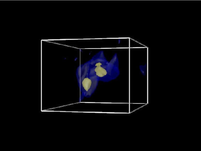
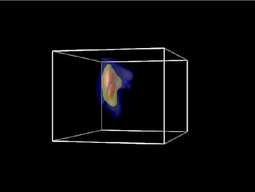
Figure 6: Iso-density surface 3D map of the clump-core system appearing at early times in run M10J4$\beta$.1, detailed in fig.  7. The times shown are a) $t=0.06t_{\rm s}$ (frame 30 in the animation of fig. 5a ) and b) $t=0.08t_{\rm s}$ (frame 40). The iso-density surfaces are at $n=10n_{0}$ (blue), $n=40n_{0}$ (yellow) and $n=100n_{0}$ (red). The latter does not exist at frame 30.

Now we focus on the evolution of the first collapsing object. From the animation in fig. 5a, we see that the collapsing core actually forms from the merger of two previous cores, which had formed almost simultaneously at frame 36 within a clump located near the center of the computational box. The two cores merge at frame 44, which marks the “birth” of the collapsing core, all happening within the larger clump. Thus, we investigate the criticality and stability of both the “parent” clump and the “daughter” cores at frames 30, 40 and 50. Figures 6a and 6b respectively show 3D iso-density surface maps of the clump/core system in question at frames 30 ($t=1.2$ Myr) and 40 ($t=1.6$ Myr). The iso-surfaces are drawn at densities $n=10n_{0}$ (blue), $n=40n_{0}$ (yellow) and $n=100n_{0}$ (red).

At frame 30 (fig. 6a), it is seen that the $n=100n_{0}$ iso-surface does not exist, since the peak density is $<100n_{0}$. It is also seen that the $n=10n_{0}$ isosurface defines a single structure, which we refer to as the parent “clump”, while the $n=40n_{0}$ isosurface resolves the two cores. At frame 40 (fig. 6b), the $n=40n_{0}$ isosurface does not resolve the two daughter cores anymore, although the $n=100n_{0}$ isosurface still does. It is important to remark that the isosurfaces drawn at a certain value of $n_{\rm t}$ at different times do not trace the same gas parcels; i.e., the isodensity surfaces are not Lagrangian boundaries. Neither are clump boundaries defined by means of standard clump-finding algorithms.

Figure 7 shows the evolution of the mass-to-flux ratio (panel a) and of the Jeans number (panel b) for this collapsing object from frame 30 to frame 50 ($t=1.2$ to 2 Myr). Three curves are shown in each panel, each corresponding to different values of the clump-defining threshold density $n_{\rm t}$. Note that two cores exist at frame 30 for $n_{\rm t}=40n_{0}$, but their $\mu_{\rm c}$ and $J_{\rm c}$ are nearly identical, and so they are described by the same (dotted) line. Similarly, at frame 40 there are two cores defined by the $n_{\rm t}=100n_{0}$ level, and in this case their $\mu_{\rm c}$ and $J_{\rm c}$ are different, so they are described by two separate (dashed) lines, which in fact start at frame 40, because the cores did not exist at threshold $n_{\rm t}=100n_{0}$ at frame 30.

From fig. 7 it is seen that that the parent clump is already Jeans-unstable and magnetically supercritical at frame 30, even though it contains two well-defined substructures, both of which individually are subcritical and sub-Jeans at this time, and are therefore probably not collapsing themselves at this time. In this sense, the merger of the two cores can be considered a part of the global collapse of the larger structure, a fact which is confirmed by noting that in the animation, the size of the $n=10n_{0}$ isosurface is also shrinking, implying that most of the mass in the whole clump is involved in the collapse (see also fig. 6).

Note that the super-Jeans and supercritical character of the $n_{\rm t}=10n_{0}$ clump at frame 30 cannot be attributed to numerical diffusion, as its mean density is only $\sim 20n_{0}$, with its peak only reaching $83n_{0}$, thus very safely below even the most stringent (and probably excessive) resolution constraint of Heitsch et al. (2001) of $n_{\rm res}=114n_{0}$. This is also supported by the fact that at this time the mass-to-flux ratio of the clump, albeit supercritical, is still smaller than that of the whole box, in agreement with the constraint that no structure within the simulation can have a value of $\mu$ larger than that of the whole box under ideal MHD. The latter property holds also for the two cores defined by $n_{\rm t}=100n_{0}$ at frame 40, whose mean and peak densities are respectively $\langle n_{1}\rangle=153n_{0}$, ${n_{\rm peak}}_{1}=337n_{0}$ and $\langle n_{2}\rangle=121n_{0}$, ${n_{\rm peak}}_{2}=166n_{0}$. It is only at frame 50, when the core has a peak density of over $5000n_{0}$ and an average density of $329n_{0}$ (above $n_{\rm t}=40n_{0}$), that its mass-to-flux ratio exceeds that of the box, indicating that at this time numerical diffusion has clearly caused significant loss of magnetic flux. However, the collapse was initiated when the whole structure was cleanly resolved, and therefore must be considered a robust physical result. That is, the formation of a supercritical, super-Jeans structure causes collapse and ultimately numerical diffusion, rather than the collapse being an artifact of numerical diffusion. The same happens during the formation and collapse of the other two collapsed cores (at frames 130 and 210). This conclusion is also supported by the fact that no collapse occurs in the subcritical simulation, even though it is only marginally so ($\mu=0.9$), which shows that the simulations accurately do not allow collapse when it physically should not occur.

Finally, two more points are worthy of notice. One is that this first collapsing object goes from first appearance to a fully collapsed state in less than $2t_{\rm fc}$, where $t_{\rm fc}\equiv L_{\rm J,c}/c$ is the local free-fall time in the core, with $L_{\rm J,c}$ being the Jeans length at the core’s mean density. At a mean density $\langle n\rangle_{\rm c}=100n_{0}$, $t_{\rm fc}=0.5{\rm Myr}=12.5$ frames. The collapse corresponds to the rapid rise of $n_{\rm max}$ from $\sim 10^{2}$ to $\sim 10^{4}n_{0}$ in fig. 2. The second is that, as in the non-magnetic case, moderate-density ($n_{\rm peak}\gtrsim 10^{2}$ cm^-3) clumps arise that redisperse on time scales 1/2–1 $t_{\rm fc}$ ($\lesssim 10$ frames).

5.2.3 Strongly supercritical case

In the strongly supercritical run M10J4$\beta$1 (fig. 5b), collapsing objects undergo a very similar evolution as in the moderately supercritical one, M10J4$\beta$.1. However, this run exhibits an additional interesting phenomenon: Besides the rapidly-collapsing dense cores and the rapidly-dispersing intermediate density clumps discussed above, we also observe the formation of two long-lasting, intermediate-density clumps ($n_{\rm peak}$ 200–300 cm^-3) which do not collapse, but which take times $\sim 0.15~{}t_{\rm s}$ ($\sim 0.6~{}t_{\rm fg}$, $\sim 75$ frames, or $\sim 3$ Myr) to redisperse. These are seen as the long-lasting clumps that do not have a red isodensity surface in the animation. One of them is formed at frame 16 ($t=0.64$ Myr) near the top of the simulation, and disperses around frame 84 ($t=3.36$ Myr). The other one forms at frame 42 ($t=1.68$ Myr) towards the left of the simulation, at roughly half the box height, and disperses around frame 120 ($t=4.80$ Myr). These clumps are marginally resolved according to the Jeans criterion, but nevertheless end up redispersing, rather than collapsing, suggesting that numerical diffusion of the magnetic field is not a concern yet in these clumps.

These clumps last a time about twice the longest durations seen in the subcritical case, and moreover have very well-defined identities, contrary to the situation in the subcritical case. It is thus interesting to investigate their physical properties. Figure 8 shows the evoulution of $\mu_{\rm c}$ and $J_{\rm c}$ for the first of these clumps from frame 20 to frame 70 ($t=0.5$ to $t=3.$ Myr). It can be seen that this core is supercritical ($\mu>1$), but sub-Jeans ($J_{\rm c}<1$) at all times and values of the core-defining threshold density $n_{\rm t}$, except at frame 20 and $n_{\rm t}=10n_{0}$, at which $J_{\rm c}$ is marginally larger than 1. Given the approximate nature of our calculations (recall the core’s radius is defined assuming a spherical geometry), and that turbulent support is not included in our analysis, we consider that the value $J_{\rm c}=1.06$ found at that particular time and density threshold is still consistent with the core not undergoing collapse in practice. We conclude that these somewhat longer-lived, non-collapsing cores come very close to collapse, but miss it, explaining their longer lifetimes in terms of our estimate of §3.2. It appears unlikely that the inclusion of AD in the calculations could help these cores to collapse, as they are already supercritical, and so their support is mainly thermal.

It is also interesting that these longest-lived cores arise in the most strongly supercritical simulation, in which the magnetic support is weakest. A possible explanation is that, somewhat counterintuitively, turbulent flows with weak magnetic fields tend to develop more moderate density fluctuations than either non-magnetic or strongly magnetized ones, as has been observed by various groups (Passot et al. 1995; Ostriker et al. 1999; Heitsch et al. 2001; Ballesteros-Paredes & Mac Low 2002). Thus, the production of moderate-amplitude density fluctuations that can “land” close to equilibrium without directly overshooting to collapse may be more likely in the weak-field case.

5.2.4 Non-magnetic simulation

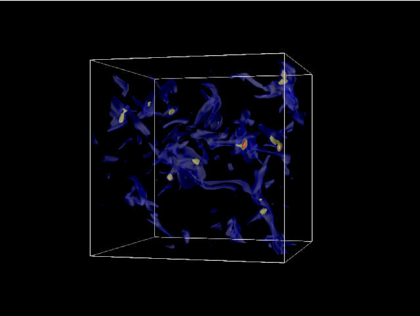
Figure 9: Animation of the non-magnetic simulation M10J4$\beta$$\infty$. The still frame in the paper edition shows the final frame (#44) of the animation. Note the larger number of cores in comparison to either supercritical run.

Figure 9 shows an animation of the nonmagnetic run M10J4$\beta$$\infty$. This simulation stops after only 45 frames, indicating that the collapse is more violent than in the magnetic cases. We can only give lower bounds to the clump lifetimes in this case, and a more detailed description must await a more robust handling scheme for the collapsed objects, to be presented elsewhere.

Two features are worth noting here. First, a significantly larger number of collapsed objects and clumps have formed by the end of the run than at the same time in either MHD run. This result must be considered preliminary only, as it is necessary to verify that the larger number of cores is a real effect, and not just a statistical fluctuation. For example, Heitsch et al. (2001) reported that the statistical fluctuations between realizations with identical parameters but different random initial conditions and driving were larger than the systematic differences between magnetic and non-magnetic cases. However, they did not discuss the number of cores formed in their simulations. The difference in core number between the magnetic and non-magnetic runs in our simulations is, however, striking, and we plan to investigate this in a forthcoming paper considering mean trends with the global parameters for ensembles of simulations.

The second point to note is that the time scales from formation to full collapse seem to cover a wider range, of $\sim 1/2$ to 1 Myr, with the fastest-collapsing objects being those that involve collisions of clumps. Moreover, a population of non-collapsed objects is seen by the end of the run for which we cannot observe the final fate nor the corresponding time scale. Several re-expanding clumps are also observed. The investigation of these trends must also await a more robust handling scheme for the sink cells.

Nevertheless, these preliminary results lead us to speculate that the presence of a magnetic field can further reduce the efficiency of collapsed-object formation in comparison with that of an equivalent non-magnetic case mostly by reducing the probability of core formation, rather than by significantly delaying the collapse of individual objects.

6 Discussion, implications and caveats

Several interesting points can be noted about the results described above:

1. Our results suggest that, at least under the assumptions of our numerical simulations, molecular cloud clumps and cores are in general likely to be dynamic, out-of-equilibrium structures, rather than quasi-hydro/magneto-static structures. This is however not in conflict with observations, as several studies show that synthetic observations of the clouds and the clumps within them in numerical simulations compare favorably to observations (e.g., Padoan et al. 1999, 2003; Klessen 2001; Ostriker et al. 2001; Ballesteros-Paredes & Mac Low 2002; Gammie et al. 2003; Klessen, Ballesteros-Paredes, Vázquez-Semadeni & Durán 2004; Schmeja & Klessen 2004). In particular, dynamically-formed cores can have angle-averaged column density profiles that resemble that of a BE-sphere (Ballesteros-Paredes, Klessen & Vázquez-Semadeni 2003), or in fact various other functional forms (Harvey et al. 2003). This is because much detail is lost by the line-of-sight and angle averaging.

2. The clump/core lifetimes that we have found in this paper (1/2-1 Myr for collapsing objects, 1/2-3 Myr for non-collapsing ones) also compare favorably with observational estimates of core lifetimes, such as those of Lee & Myers (1999), who obtained estimated lifetimes of 0.3-1.6 Myr. However, an interesting remark is in order. Lee & Myers obtained those estimates under the assumption that all cores undergo AD-mediated contraction, infall, and then protostellar emission, so that the number of starless cores ($n_{\rm SL}$) and of cores with young stellar objects (YSOs) ($n_{\rm YSO}$) are respectively proportional to the time spent in the prestellar and protostellar epochs during this process. However, our results advocate the possibility that not all clumps undergo collapse, and in this case it is easy to show that the ratio $n_{\rm SL}/n_{\rm YSO}$ is an upper bound to the lifetime ratio. Indeed, define $e\equiv n_{\rm SL}/n_{\rm YSO}$. If the number of starless cores comprises a fraction $\epsilon$ of failed cores and a fraction $1-\epsilon$ of true pre-stellar cores (with number $n_{\rm PS}$), then

$$e\equiv\frac{n_{\rm SL}}{n_{\rm YSO}}=\frac{n_{\rm PS}}{n_{\rm YSO}}\left(\frac{1}{1-\epsilon}\right).$$ (10)

Now, since the ratio of true pre-stellar objects to proto-stellar ones is indeed equal to the ratio of pre-stellar to protostellar lifetimes $\tau_{\rm PS}/\tau_{\rm YSO}$, we find

$$e=\frac{\tau_{\rm PS}}{\tau_{\rm YSO}}\left(\frac{1}{1-\epsilon}\right)>\frac{\tau_{\rm PS}}{\tau_{\rm YSO}},$$ (11)

which is the desired result. Although the actual fraction of failed cores has not been quantified in our numerical simulations (again, ensembles of simulations are needed), and is unknown in the observations, this consideration is consistent with the fact that the longest lifetimes of collapsing objects in our simulations are shorter by a factor of $\sim 2/3$ than the upper bound of Lee & Myers’ (1999) estimates.

3. It is important to compare the fraction of collapsing versus non-colapsing clumps in the simulations with observational data. This will be attempted in detail in a separate paper, but here we can give the following simple estimate. Assuming that a minimum number density of $\sim 10^{4}$ cm^-3 is necessary to excite a high-density tracer such as ammonia, a typical “ammonia core” consists of the “tip of the iceberg” region of a clump above this minimum density. Such minimum density can be identified with our core-defining threshold density $n_{\rm t}$, giving $n_{\rm t}\sim 20n_{0}$. In our simulations, typical failed, re-expanding cores defined with this value of $n_{\rm t}$ only reach mean densities of up to 2–3 times $n_{\rm t}$ ($\sim 50n_{0}=2.5\times 10^{4}$ cm^-3). Thus, it seems that most of the re-expanding clumps and cores in our simulations would lie below the ammonia detection limit, and would preferentially appear in lower-density-tracer surveys, while surveys in high-density tracers such as ammonia may tend to preferentially select collapsing objects. Detailed synthetic observations of the simulations with various clump-defining density thresholds are necessary to determine whether the observed fraction of inward versus outwards (i.e., contracting vs. re-expanding) motions in cores (e.g., Lee, Myers & Tafalla 2001) are well reproduced by the simulations.

4. In the analysis of §5.2, we have neglected turbulent support of the clumps and cores. Interestingly, the ($J_{\rm c},\mu_{\rm c}$) parameter space seems to describe very well the outcome of the clump/core system evolution. This may be because at the small sizes of these objects, the internal turbulence may be of secondary importance. Indeed, real cores are typically transonic or even subsonic, a feature reproduced by the simulations (Klessen et al. 2004). In this case, the turbulent support is comparable or smaller than the thermal support, and so only the magnetic and thermal supports remain for consideration.

5. The caveat that our results hold only within the realm of the assumptions described in §2 should be stressed. Although in that section we have referred to observational evidence suggestive that the numerical setup and parameters used in this paper are the most realistic (except for the neglect of AD), the issue of whether molecular clouds are nearly isothermal, continually driven and supercritical is still unsettled. Our clump lifetimes in the subcritical case are short because the turbulence is continually driven. We cannot overemphasize the importance of continued observational surveys directed at determining the true conditions in molecular clouds, or the fraction of clouds under each type of condition. Also, numerical simulations of the interstellar medium at large, in which the formation of molecular clouds is accurately simulated, can shed light on this issue.

7 Summary and conclusions

In this paper we have discussed the lifetimes of clumps and cores in both the non-magnetic and magnetic cases, in single-phase, isothermal, turbulent models of molecular clouds. Under these conditions, we have remarked that, in the non-magnetic case, the hotter, low-density gas necessary for the confinement of stable BE-type hydrostatic configurations is absent, and so we do not expect these structures to form out of transient turbulent fluctuations in the clouds. We have then given a qualitative discussion suggesting that non-truncated (“extended”) isothermal structures may be expected to be unstable in general, in agreement with the fact that non-magnetic polytropic simulations with $\gamma_{\rm e}<4/3$ do not form hydrostatic structures (e.g., Vázquez-Semadeni et al. 1996; Klessen et al. 2000; Bate et al. 2003; Li et al. 2003). Thus, we have suggested that in the non-magnetic case, clumps should be expected to be completely transient structures, either proceeding to collapse right away upon the turbulent compression that formed them, or else re-expanding to merge back into their environment (“failed” clumps).

For failed clumps, we have given a simple estimate for the characteristic re-expansion time, as slowed down by the self-gravity of the clump, finding times $\sim$ a few clump free-fall times, comparable to the lifetime estimates of Lee & Myers (1999). The longest lifetimes correspond to re-expanding clumps that come very close to equilibrium between self-gravity and thermal pressure. In general, failed clumps are not destined to form stars. However, in the simulations there is always a population of these clumps present, in agreement with some observational suggestions (Taylor et al. 1996). These can be associated with at least part of the observed starless cores, which traditionally have been thought of as being in a pre-stellar phase.

In the magnetic case, we have presented a set of of driven-turbulence, ideal-MHD numerical simulations focusing on the lifetimes and criticality of the individual clumps and cores in relation to the conditions in their parent clouds. We have found that:

a) Magnetostatic clumps do not form in the case of subcritical environments; the clumps that form in this case have mean densities $\bar{n}\sim$ 10–100$n_{0}$ ($5\times 10^{3}$–$5\times 10^{4}$ cm^-3), and lifetimes $\sim$ 0.2–1.3 Myr, ultimately being dispersed by the turbulence in the environment. A few of these clumps nevertheless become moderately gravitationally bound, being the ones with the longest lifetimes. An estimate of the AD time scale in these clumps gives characteristic times $\gtrsim 1.3$ Myr, suggesting that they can marginally be “captured” by AD and increase their mass-to-flux ratio before they can be dispersed, thus increasing their gravitational binding, to eventually become supercritical and collapse. Thus, they adjust to the standard model scenario, except for the fact that with these time scales, AD does not significantly increase the cores’ lifetimes in comparison to those of supercritical or non-magnetic ones. This questions the usefulness of AD-mediated contraction as a SFE-decreasing agent in the standard model, and the criticality of the parent may become irrelevant for the formation of supercritical cores in short time scales.

b) In the supercritical case, dense cores ($\bar{n}\sim$ 100–1000 $\times n_{0}$, or $5\times 10^{5}$–$5\times 10^{6}$ cm^-3 do form, being supercritical since their early stages and collapsing on time scales $\sim 2t_{\rm fc}\sim 1$ Myr. Ambipolar diffusion is not required for collapse in this case, as the objects rapidly become supercritical by the turbulent compressions themselves, since there is a large enough mass reservoir around them. The lifetimes in the magnetic case are in general again in agreement with the observational estimates of Lee & Myers (1999) and our own simple, non-magnetic estimate.

c) As in the non-magnetic case, coexisting with the collapsing cores, numerous lower-density ($\bar{n}\lesssim 100n_{0}$) “failed” ones form and disperse in times comparable to their free-fall times. These “failed” clumps include the longest-lived objects observed in our simulations, again in agreement with our simple calculation, which suggests that the longest lifetimes correspond to re-expansion from states very close to equilibrium. However, it appears unlikely that the inclusion of ambipolar diffusion could induce their collapse, as these objects are already supercritical, and the reason they do not collapse is because they do not manage to become gravitationally unstable with respect to the thermal support.

Within the framework of our assumptions, our results support the developing notion that star formation is a dynamic process, in which the only hydrostatic configurations may be the stars themselves.

Table 1: Numerical simulation parameters.

Run name	$M_{\rm s}$	$J$	$\beta$	Resolution	$L$(pc)	$n_{0}$(cm-3)	$B_{0}$($\mu$G)	$\sigma$(km s-1)	$\mu$
M10J4$\beta$$\infty$	10	4	$\infty$	$256^{3}$	4	500	0.0	2.0	$\infty$
M10J4$\beta$1	10	4	1	$256^{3}$	4	500	4.6	2.0	8.8
M10J4$\beta$.1	10	4	0.1	$256^{3}$	4	500	14.5	2.0	2.8
M10J4$\beta$.01	10	4	0.01	$256^{3}$	4	500	45.8	2.0	0.9
M10J4$\beta$.01LR	10	4	0.01	$128^{3}$	4	500	45.8	2.0	0.9
M10J3$\beta$.01	10	3	0.01	$128^{3}$	4	281	34.4	2.0	0.7
M8J4$\beta$.1	8	4	0.1	$128^{3}$	2.56	1220	22.6	1.6	2.8
M8J4$\beta$.01	8	4	0.01	$128^{3}$	2.56	1220	71.6	1.6	0.9

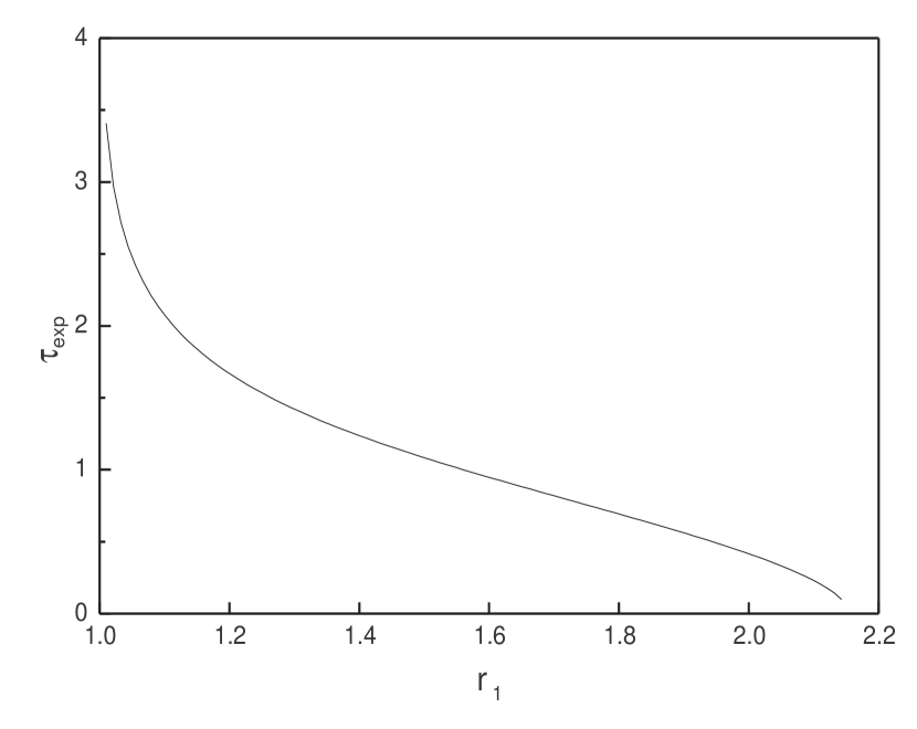
Figure 1: a) (Left panel) Re-expansion time of a core, in units of the free-fall time, defined as the time necessary to double its initial radius, as a function of the initial radius $r_{1}$, normalized to the equilibrium radius. b) (Right panel) Simulated “observer’s perspective” of the re-expansion time, giving the time to go from the initial radius $r_{1}$ to a final one with density $0.1~{}\rho_{\rm e}$, where $\rho_{\rm e}$ is the density of the equilibrium configuration. This emulates the time the core would be visible to a high-density tracer sensitive to densities $>0.1\rho_{\rm e}$.

Figure 2: Time-evolution of the global maximum of the density field for runs M10J4$\beta$.01 (dotted line), M10J4$\beta$.1 (solid line), M10J4$\beta$1 (short-dashed line) and M10J4$\beta$$\infty$ (long-dashed line). The numbers indicate the corresponding values of $\beta$. The upper time-axis is given in units of the global free-fall time of the simulation.

Figure 4: Evolution of the mass-to-flux ratio (in units of the critical value) $\mu_{\rm c}$ and of the Jeans number $J_{\rm c}$ for the densest, moderately long-lived core in the subcritical run M10J4$\beta$.01. The lower time-axis is given in units of the frame number in the animation.

Figure 7: Evolution of: (Left panel) the mass-to-flux ratio (in units of the critical value) $\mu_{\rm c}$ and of (right panel) the Jeans number $J_{\rm c}$ for the first collapsing object in the moderately supercritical run M10J4$\beta$.1. The various curves correspond to different values of the clump-defining threshold density $n_{\rm t}$. Note that at frame 40 there are two cores defined by $n_{\rm t}=100n_{0}$, described by the two dashed lines. At frame 30 the peak density is below $100n_{0}$ and therefore the dashed lines do not extend down to this frame. Note also that at frame 30 there are two cores defined by $n_{\rm t}=40n_{0}$, but their $\mu_{\rm c}$ and $J_{\rm c}$ are nearly idenstical, and so only one curve is shown.

Figure 8: Evolution of: (left panel) the mass-to-flux ratio (in units of the critical value) $\mu_{\rm c}$ and of (right panel) the Jeans number $J_{\rm c}$ for the first long-lived rebounding clump in the strongly supercritical run M10J4$\beta$1. The curve coding is as in fig. 7. Note that this clump is always supercritical, but almost always sub-Jeans. The failure to collapse even though $J_{\rm c}$ is slightly above unity for $n_{\rm t}=10n_{0}$ at frame 20 can be understood in terms of the non-accounting for turbulent support, and also slight imprecisions in our estimates of the core parameters (see text).

Appendix A Ambipolar diffusion time scale in a subcritical clump

Here we estimate the ambipolar diffusion (AD) time scale $\tau_{\rm AD}$ under the conditions of the longest-lived clump in the subcritical run M10J4$\beta$.01. To this end, we use the formulas given by Fiedler & Mouschovias (1992). They write

$$\tau_{\rm AD}=\frac{8}{1.4\pi^{2}}\frac{\tau_{\rm ff}^{2}}{\tau_{\rm ni}}\left(1-\frac{8}{\pi^{2}}\frac{\tau_{\rm ff}^{2}}{\tau_{\rm s}^{2}}\right)^{-1},$$ (A1)

where $\tau_{\rm s}\equiv R_{\rm c}/c_{\rm s}$ is the sound crossing time and $\tau_{\rm ff}$ is free-fall time scale

$$\tau_{\rm ff}=\left(\frac{3\pi}{32G\rho_{\rm n}}\right)^{1/2}.$$ (A2)

Note that this definition of the free-fall time is smaller by a factor of $\sqrt{3/32}$ than that used in the main body of this paper. This, however, causes no inconsistency, as we compare the AD time scale and core lifetimes in physical units. Finally, $\tau_{\rm ni}$ is the neutral-ion collision time scale, given by

$$\tau_{\rm ni}=\frac{m_{\rm i}+m_{\rm n}}{\rho_{\rm i}\langle\sigma w\rangle_{\rm in}},$$ (A3)

in which $m_{\rm n}$ and $m_{\rm i}$ are the neutral and ion particle masses, respectively, $\rho_{\rm n}$ and $\rho_{\rm i}$ the neutral and ion mass densities, and $\langle\sigma w\rangle_{\rm in}$ is the neutral-ion collision rate. We can write the above equation as

$$\tau_{\rm ni}=\frac{1+\frac{m_{\rm n}}{m_{\rm i}}}{n_{\rm i}\langle\sigma w\rangle_{\rm in}}.$$ (A4)

Fiedler & Mouschovias also give an approximate expression for the ion number density as

$$n_{\rm i}\approx K\left(\frac{n_{\rm n}}{10^{5}{\rm cm}^{-3}}\right)^{k},$$ (A5)

with canonical values $K=3\times 10^{-3}$ cm^-3, $k=1/2$, and $\langle\sigma w\rangle_{\rm in}=1.69\times 10^{-9}{\rm cm}^{3}{\rm s}^{-1}$. We also take $m_{\rm i}\sim 29.0m_{\rm H}$ and $m_{\rm n}=2.36m_{\rm H}$, with $m_{\rm H}=1.67\times 10^{-24}$ g.

Defined out to a threshold density $n_{\rm t}=40n_{0}$, the core in question has a mean density of $55n_{0}=2.75\times 10^{4}$ cm^-3 at the time when it attains the maximum value of its mass-to-flux ratio, $\mu_{\rm c,max}=0.28$ (see fig. 4). This core is highly flattened, and thus we compute its radius as the maximum distance between the density maximum and the clump’s periphery (cf. §4.3), finding $R_{\rm c}=0.3$ pc. With these values we thus obtain $\tau_{\rm ni}=1.29\times 10^{4}$ yr, $\tau_{\rm ff}=2.02\times 10^{5}$ yr, $\tau_{\rm s}=1.5\times 10^{6}$ yr, and $\left[1-(8/\pi^{2})(\tau_{\rm ff}/\tau_{\rm s})^{2}\right]^{-1}=1.015$. Substituting in eq. (A1) we finally obtain

$$\tau_{\rm AD}\approx 9.2\tau_{\rm ff}=1.9~{}{\rm Myr}.$$ (A6)

This estimate is very close to the simpler, more general estimate often quoted (e.g., Ciolek & Basu 2001) of $\tau_{\rm AD}\approx\tau_{\rm ff}^{2}/(1.4\tau_{\rm ni})=11.2\tau_{\rm ff}=2.3$ Myr.

A correction to this estimate to take into account the initial value of the mass-to-flux ratio in the core, $\mu_{\rm c}$ has recently been given by Ciolek & Basu (2001). From their fig. 1 and the value $k=1/2$ that we have used here, the correction factor is $C(\mu_{\rm c0})\sim 0.7$. This is the smallest possible value of their correction factor at this value of $\mu_{\rm c}$. So we conclude that

$$\tau_{\rm AD}\gtrsim 1.3~{}{\rm Myr}.$$ (A7)

References

- (1)
- (2) Alves, J. F., Lada, C. J., & Lada, E. A. 2001, Nature 409, 159
- (3)
- (4) Ballesteros-Paredes, J. 2004, in From Observations to Self-Consistent Modeling of the Interstellar Medium, eds. M. de Avillez and D. Breitschwerdt (Dordrecht: Kluwer), 67
- (5)
- (6) Ballesteros-Paredes, J., & Vázquez-Semadeni, E. 1997, in “Star Formation, Near and Far. 7th Annual Astrophysics Conference in Maryland”, ed. S. Holt and L. Mundy (New York: AIP Press ), p.81
- (7)
- (8) Ballesteros-Paredes, J., Vázquez-Semadeni, E., & Scalo, J. 1999a, ApJ, 515, 286
- (9)
- (10) Ballesteros-Paredes, J., Hartmann, L. & Vázquez-Semadeni, E. 1999b, ApJ 527, 285
- (11)
- (12) Ballesteros-Paredes, J. & Mac Low, M. 2002, ApJ, 570, 734
- (13)
- (14) Ballesteros-Paredes, J., Klessen, R. & Vázquez-Semadeni, E. 2003, ApJ 592, 188
- (15)
- (16) Bania, T.M. & Lyon, J.G. 1980, ApJ 239, 173
- (17)
- (18) Bate, M. R., Bonnell, I. A., & Bromm, V. 2002, MNRAS 336, 705
- (19)
- (20) Blitz, L., 1993, in “Protostars and Planets III”, eds. E. H. Levy and J. I. Lunine (Tucson: Univ. of Arizona Press), 125
- (21)
- (22) Blitz, L., & Williams, J P. 1999, in “The Origin of Stars and Planetary Systems”, ed. C. J. Lada and N. D. Kylafis (Dordrecht: Kluwer), 3
- (23)
- (24) Bonnor, W. B. 1956, MNRAS, 116, 351
- (25)
- (26) Bourke, T. L., Myers, P. C., Robinson, G., Hyland, A. R. 2001, ApJ 554, 916
- (27)
- (28) Brunt, C. M., & Heyer, M. H. 2002, ApJ 566, 289
- (29)
- (30) Brunt, C. M. 2003, ApJ 583, 280
- (31)
- (32) Ciolek, G. E. & Basu, S. 2001, ApJ 547, 272
- (33)
- (34) Clark, P. C. & Bonnell, I. A. 2004, MNRAS, in press (astro-ph/0311286)
- (35)
- (36) Clarke, C. J. & Pringle, J. E. 1997, MNRAS 288, 674
- (37)
- (38) Chandrasekhar, S. 1961, Hydrodynamic and Hydromagnetic Stability (New York: Dover)
- (39)
- (40) Chandrasekhar, S., & Fermi, E. 1953, ApJ, 118, 116
- (41)
- (42) Crutcher, R. M. 1999, ApJ 520, 706
- (43)
- (44) Crutcher, R. 2004, in “Magnetic Fields and Star Formation: Theory versus Observations”, eds. Ana I. Gomez de Castro et al, (Dordrecht: Kluwer Academic Press), in press
- (45)
- (46) Crutcher, R., Heiles, C. & Troland, T. 2002, in Simulations of Magnetohydrodynamic Turbulence in Astrophysics, ed. T. Passot & E. Falgarone (Berlin: Springer), 155
- (47)
- (48) Curry, C. L. 2000, ApJ, 541, 831
- (49)
- (50) Ebert, R. 1955, Zeitschrift für Astrophysik, 36, 222
- (51)
- (52) Elmegreen, B. G. 1993, ApJ, 419, L29
- (53)
- (54) Evans, N. J., II 1999, ARAA 37, 311
- (55)
- (56) Evans, N. J., Rawlings, J. M. C., Shirley, Y. L., & Mundy, L. G. 2001, ApJ, 557, 193
- (57)
- (58) Fiedler, R. A. & Mouschovias, T. Ch. 1992, ApJ 391, 199
- (59)
- (60) Field, G. B., Goldsmith, D. W., & Habing, H. J. 1969, ApJ,155, L149
- (61)
- (62) Gammie, C. F., Lin, Y.-T., Stone, J. M., & Ostriker, E. C. 2003, ApJ 592, 203
- (63)
- (64) Gazol, A., Passot, T. & Sulem, P. L. 1999, Phys. Plasmas 6, 3114
- (65)
- (66) Gilden, D. L. 1984, ApJ 283, 679
- (67)
- (68) Goldsmith, P. F. 1987, in Interstellar Processes, eds./ D. J. Hollenbach and H. A. Thronson (Dordrecht: Reidel), 51
- (69)
- (70) Hartmann, L., Ballesteros-Paredes, J., & Bergin, E. A. 2001, ApJ, 562, 852
- (71)
- (72) Harvey, D. W. A., Wilner, D. J., Lada, C. J., Myers, P. C., Alves, J., & Chen, H. 2001, ApJ, 563, 903
- (73)
- (74) Harvey, D. W. A., Wilner, C. J., Myers, P. C. & Tafalla, M. 2003, ApJ 597, 424
- (75)
- (76) Hayashi, C. 1966, AR&A 4, 171
- (77)
- (78) Heitsch, F., Mac Low, M. M., & Klessen, R. S. 2001, ApJ, 547, 280
- (79)
- (80) Heyer, M. H. & Brunt, C. M. 2004, ApJ, submitted
- (81)
- (82) Hunter, C. 1977, ApJ 218, 834
- (83)
- (84) Hunter, J. H., Jr., Sandford, M. T., II, Whitaker, R. W., Klein, R. I. 1986, ApJ 305, 309
- (85)
- (86) Jijina, J., Myers, P. C., & Adams, F. C. 1999, ApJS 125, 161
- (87)
- (88) Johnstone, D., Wilson, C. D., Moriarty-Schieven, G., Joncas, G., Smith, G., Gregersen, E., & Fich, M. 2000, ApJ, 545, 327
- (89)
- (90) Kim, J., Ryu, D., Jones, T. W. & Hong, S. S. 1999, ApJ 514, 506
- (91)
- (92) Kim, J., Balsara, D. & Mac Low, M.-M. 2001, JKAS 34, S333
- (93)
- (94) Klessen, R. S., Heitsch, F., & MacLow, M. M. 2000, ApJ, 535, 887
- (95)
- (96) Klessen, R. S. 2001, ApJ 556, 837
- (97)
- (98) Klessen, R. S., Ballesteros-Paredes, J., Vázquez-Semadeni, E. C. & Durán, C. 2004, ApJ, submitted (astro-ph/0306055)
- (99)
- (100) Koyama, H. & Inutsuka, S.-I. 2002, ApJ 564, L97
- (101)
- (102) Larson, R. B. 1969, MNRAS, 145, 271
- (103)
- (104) Larson, R. B. 1981, MNRAS, 194, 809
- (105)
- (106) Larson, R. B. 1985, MNRAS, 214, 379
- (107)
- (108) Lee, C. W. & Myers, P. C. 1999, ApJS 123, 233
- (109)
- (110) Lee, C. W., Myers, P. C. & Tafalla, M. 2001, ApJS 136, 703
- (111)
- (112) Li, P. S., Norman, M. L., Mac Low, M.-M. & Heitsch, F. 2004, ApJ 605, 800
- (113)
- (114) Li, Y., Kleesen, R. S. & Mac Low, M.-M. 2003, ApJ 592, 975
- (115)
- (116) Li, Z.-Y. & Nakamura, F. 2004, ApJL, in press (astro-ph/0405615)
- (117)
- (118) Lizano, S., & Shu, F. H. 1989, ApJ, 342, 834
- (119)
- (120) Lombardi, M. & Bertin, G. 2001, A&A, 375, 1091
- (121)
- (122) Low, C. & Lynden-Bell, D. 1976, MNRAS 176, 367
- (123)
- (124) Mac Low, M.-M. & Klessen, R. S. 2004, Rev. Mod. Phys. 76, 125
- (125)
- (126) Maddalena, R. J. & Thaddeus, P. 1985, ApJ 294, 231
- (127)
- (128) Masunaga, H. & Inutsuka, S.-I. 1999, ApJ 510, 822
- (129)
- (130) McKee, C. F., Zweibel, E. G., Goodman, A. A. & Heiles, C. 1993, in Protostars and Plantes III, eds. E.H. Levy and J.I. Lunine (Tucson: Univ. of Arizona Press), p. 327
- (131)
- (132) McLaughlin, D. E., & Pudritz, R. E. 1996, ApJ, 469, 194
- (133)
- (134) Mestel, L., Spitzer, L., Jr. 1956, MNRAS 116, 503
- (135)
- (136) Mouschovias, T. C. 1976a, ApJ 207, 141
- (137)
- (138) Mouschovias, T. C. 1976b, ApJ 206, 753
- (139)
- (140) Mouschovias, T. C. & Spitzer, L., Jr. 1976, ApJ 210, 326
- (141)
- (142) Myers, P. C. 1978, ApJ 225, 380
- (143)
- (144) Nakano, T. & Nakamura, T. 1978, PASJ 30, 671
- (145)
- (146) Nakano, T. 1998, ApJ 494, 587
- (147)
- (148) Ossenkopf, V. & Mac Low, M.-M. 2002, A&A 390, 307
- (149)
- (150) Ostriker, J. 1964, ApJ 140, 1056
- (151)
- (152) Ostriker, J. 1965, ApJS 11, 167
- (153)
- (154) Ostriker, E. C., Gammie, C. F. & Stone, J. M. 1999, ApJ 513, 259
- (155)
- (156) Ostriker, E. C., Stone, J. M. & Gammie, C. F. 2001, ApJ 546, 980
- (157)
- (158) Padoan, P. 1995, MNRAS, 277, 377
- (159)
- (160) Padoan, P. & Nordlund, Å. 1999, ApJ 526, 279
- (161)
- (162) Padoan, P., Bally, J., Billawala, Y., Juvela, M., Nordlund, Å 1999, ApJ 525, 318
- (163)
- (164) Padoan, P., Juvela, M., Goodman, A.A., Nordlund, Å2001 ApJ 553, 227
- (165)
- (166) Padoan, P., Goodman, A. A. & Juvela, M. 2003, ApJ 588, 881
- (167)
- (168) Passot, T., Vázquez-Semadeni, E. & Pouquet, A. 1995, ApJ 455, 536
- (169)
- (170) Passot, T. & Vázquez-Semadeni, E. 2003, A&A 398, 845
- (171)
- (172) Pouquet, A., Léorat, J. & Passot, T. 1991, in Advance in Turbulence III, eds. A. Johansson and H. Alfredsson (Berlin:Springer), 343
- (173)
- (174) Pratap, P., Dickens, J. E., Snell, R. L., Miralles, M. P., Bergin, E. A., Irvine, W. M., & Schloerb, F. P. 1997, ApJ 486, 862
- (175)
- (176) Scalo, J. 1987, in Interstellar Processes, eds. D.J. Hollenbach and H.A. Thronson (Dordrecht: Reidel), p. 349
- (177)
- (178) Scalo, J., Vázquez-Semadeni, E., Chappell, D., & Passot, T. 1998, ApJ 504, 835
- (179)
- (180) Schmeja, S. & Klessen, R. S. 2004, A&A 419, 405
- (181)
- (182) Shadmehri, M., Vázquez-Semadeni, E., & Ballesteros-Paredes, J. 2002, in Seeing Through the Dust: The Detection of HI and the Exploration of the ISM in Galaxies, eds. A. R. Taylor, T. L. Landecker, and A. G. Willis (San Francisco: Astronomical Society of the Pacific), 190
- (183)
- (184) Shu, F. 1977, ApJ 214, 488
- (185)
- (186) Shu, F. H., Adams, F. C., & Lizano, S. 1987, ARA&A, 25, 23
- (187)
- (188) Spaans, M. & Silk, J. 2000, ApJ 538, 115
- (189)
- (190) Spitzer, L. 1968. Diffuse Matter in Space (New York, Wiley), §6.1
- (191)
- (192) Stone, J. M., Ostriker, E. C., & Gammie, C. F. 1998, ApJ, 508, L99
- (193)
- (194) Taylor, S. D., Morata, O., & Williams, D. A. 1996, A&A 313, 269
- (195)
- (196) Tilley, D. A. & Pudritz, R. E. 2004, MNRAS, submitted (astro-ph/0406122)
- (197)
- (198) Truelove, J. K., Klein, R. I., McKee, C. F., Hilliman, J. H. II., Howell, L. H., & Greenough, J. A. 1997, ApJ, 489, L179
- (199)
- (200) Vázquez-Semadeni, E., Passot, T., & Pouquet, A. 1996, ApJ, 473, 881
- (201)
- (202) Vázquez-Semadeni, E., Ostriker, E. C., Passot, T., Gammie, C. & Stone, J., 2000, in “Protostars & Planets IV”, ed. V. Mannings, A. Boss & S. Russell (Tucson: Univ. of Arizona Press), 3
- (203)
- (204) Vázquez-Semadeni, E. 2002, in Seeing Through the Dust: The Detection of HI and the Exploration of the ISM in Galaxies, eds. R. Taylor, T. Landecker, & A. Willis (ASP: San Francisco), 155
- (205)
- (206) Vázquez-Semadeni, E., Ballesteros-Paredes, J. & Klessen, R. 2003a, ApJ 585, L131
- (207)
- (208) Vázquez-Semadeni, E., Ballesteros-Paredes, J. & Klessen, R. 2003b, in Galactic Star Formation Across the Stellar Mass Spectrum, ASP conf. series, ed. J. M. De Buizer (San Francisco: ASP), in press (astro-ph/0206038)
- (209)
- (210) Vázquez-Semadeni, E. 2003, in Star Formation at High Angular Resolution, IAU Symposium 221, eds. M. Burton, R. Jayawardhana & T. Bourke (San Francisco: Astronomical Society of the Pacific), in press (astro-ph/0309717)
- (211)
- (212) Walder, R. & Folini, D. 1998 A&A 330, L21
- (213)
- (214) von Weizsäcker, C.F. 1951, ApJ 114, 165
- (215)
- (216) Yabushita, S. 1968, MNRAS 140, 109
- (217)
- (218) Zuckerman, B. & Evans, N. J. II 1974, ApJ 192, L149
- (219)
- (220) Zweibel, E. G. 1990, ApJ 348, 186
- (221)