Magnetically Driven Accretion Flows in the Kerr Metric IV: Dynamical Properties of the Inner Disk

Abstract

This paper continues the analysis of a set of general relativistic 3D MHD simulations of accreting tori in the Kerr metric with different black hole spins. We focus on bound matter inside the initial pressure maximum, where the time-averaged motion of gas is inward and an accretion disk forms. We use the flows of mass, angular momentum, and energy in order to understand dynamics in this region. The sharp reduction in accretion rate with increasing black hole spin reported in Paper I of this series is explained by a strongly spin-dependent outward flux of angular momentum conveyed electromagnetically; when $a/M\geq 0.9$, this flux can be comparable to the inward angular momentum flux carried by the matter. In all cases, there is outward electromagnetic angular momentum flux throughout the flow; in other words, contrary to the assertions of traditional accretion disk theory, there is in general no “stress edge,” no surface within which the stress is zero. The retardation of accretion in the inner disk by electromagnetic torques also alters the radial distribution of surface density, an effect that may have consequences for observable properties such as Compton reflection. The net accreted angular momentum is sufficiently depressed by electromagnetic effects that in the most rapidly-spinning black holes mass growth can lead to spindown. Spinning black holes also lose energy by Poynting flux; this rate is also a strongly increasing function of black hole spin, rising to $\gtrsim 10\%$ of the rest-mass accretion rate at very high spin. As the black hole spins faster, the path of the Poynting flux changes from being predominantly within the accretion disk to predominantly within the funnel outflow.

1 Introduction

In this paper, we continue the analysis of a series of simulations of accretion disks in the Kerr metric introduced in De Villiers, Hawley, & Krolik (2003; hereafter Paper I). The emphasis in this paper will be on the properties of the accretion flow inside the initial pressure maximum, where the net time-averaged motion is towards the black hole. This region of the accretion flow, in the terminology introduced in Paper I, comprises the inner part of the main disk body, the inner torus, the plunging region, and the corona. It is arguably the most important region of all in an accretion disk because it is here that most of the energy is released that ultimately powers the observed radiation and outflows. Our goal is to understand the peculiarities of dynamics in this region; our principal tool will be to analyze the flows of three conserved quantities, mass, energy, and angular momentum. By so doing, we aim to shed light on the accretion process, how it is moderated by black hole spin, and how energy and angular momentum can be extracted from the spinning black hole.

Accretion onto black holes differs from accretion onto ordinary objects in several ways, but two stand out: the absence of stable circular orbits inside of a critical radius, and the presence of frame-dragging due to black hole spin. The absence of stable circular orbits between the radius of marginal stability $r_{ms}$ and the event horizon means that in this region matter flows in rapidly and the mass surface density is much smaller than in the main disk body where matter orbits stably. We may therefore talk about the disk having an “inner edge” in the vicinity of $r_{ms}$. However, as emphasized by Krolik & Hawley (2002), where one places this inner edge depends on precisely which disk property is under consideration. For example, two distinct edges can be defined by dynamical properties: the turbulence edge, where a transition takes place in the character of magnetic field evolution—from turbulence-driven evolution in the disk proper to evolution by magnetohydrodynamic (MHD) flux-freezing, and the stress edge, within which the stress in the accreting fluid goes to zero so that there is no outward transport of angular momentum. Another two are more closely related to photon emission properties: the reflection edge, where production of Compton reflection features ceases, and the radiation edge, where intrinsic luminosity detected by distant observers goes to zero due to reduced radiative efficiency or relativistic effects. Fully relativistic simulations can explore the relation between these observable disk edges, and the detailed dynamics of the accretion flow. Defining the location and nature of these edges is central to linking disk dynamical models to disk observables because these edges determine, among other things, the global radiative efficiency of accretion.

The other salient feature of relativistic accretion is the presence of frame-dragging when the black hole spins. Frame-dragging introduces a new dynamical effect into the accretion flow, and the spin of the black hole represents a potential source of energy output beyond that of the accretion flow itself. In a previous paper of this series (De Villiers et al. 2004) we presented evidence from the simulations that black hole spin energy helps to power axial jets. Here we focus on the flow of angular momentum and energy through the disk and corona, the influence of the black hole spin on the main accretion flow, and how the character of that flow depends on that spin. We find that frame-dragging and its associated effects can have a dramatic impact on the rate of accretion, the structure of the inner disk, and the fundamental flow of energy and angular momentum.

This paper is organized as follows: After a quick summary of the simulations and the numerical diagnostics we used to study them (§2), we devote one section each to the flow through the disk of the three conserved quantities, mass (§3), angular momentum (§4), and energy (§5). In each case, we try to highlight how much goes where, how it is split between matter and electromagnetic contributions, and how the situation changes with changing black hole spin. Section 6 summarizes our findings and comments on astrophysical implications of the numerical results.

2 Preliminaries

2.1 Simulation definition

We solve the equations of ideal MHD in the metric of a rotating black hole. The specific form of the equations we solve, and the numerical algorithm incorporated into the GRMHD code are described in detail in De Villiers & Hawley (2003). For reference we reiterate here the key terms and the definitions of the primary code variables.

We work in the Kerr metric, expressed in Boyer-Lindquist coordinates, $(t,r,\theta,\phi)$, for which the line element has the form, ${ds}^{2}=g_{tt}\,{dt}^{2}+2\,g_{t\phi}\,{dt}\,{d\phi}+g_{rr}\,{dr}^{2}+g_{\theta\theta}\,{d\theta}^{2}+g_{\phi\phi}\,{d\phi}^{2}$. We use the metric signature $(-,+,+,+)$. The determinant of the 4-metric is $g$, and $\sqrt{-g}=\alpha\,\sqrt{\gamma}$, where $\alpha$ is the lapse function, $\alpha=1/\sqrt{-g^{tt}}$, and $\gamma$ is the determinant of the spatial $3$-metric. We follow the usual convention of using Greek characters to denote full space-time indices and Roman characters for purely spatial indices. We use geometrodynamic units where $G=c=1$; time and distance are in units of the black hole mass, $M$.

The state of the relativistic test fluid at each point in the spacetime is described by its density, $\rho$, specific internal energy, $\epsilon$, 4-velocity, $U^{\mu}$, and isotropic pressure, $P$. The relativistic enthalpy is $h=1+\epsilon+P/\rho$. The pressure is related to $\rho$ and $\epsilon$ through the equation of state of an ideal gas, $P=\rho\,\epsilon\,(\Gamma-1)$, where $\Gamma$ is the adiabatic exponent. For these simulations we take $\Gamma=5/3$. The magnetic field of the fluid is described by two sets of variables, the constrained transport magnetic field, $F_{jk}=[ijk]\,{\cal{B}}^{i}$, and magnetic field $4$-vector $\sqrt{4\pi}\,b^{\mu}={}^{*}F^{\mu\nu}U_{\nu}$. The ideal MHD condition requires $U^{\nu}F_{\mu\nu}=0$. The magnetic field $b^{\mu}$ is included in the definition of the total four momentum, $S_{\mu}=(\rho\,h\ +{\|b\|}^{2})\,W\,U_{\mu}$, where $W$ is the Lorentz factor. We define the transport velocity as $V^{i}=U^{i}/U^{t}$.

In Paper I we presented results of a series of high- and low-resolution simulations, the KD (Keplerian Disk) set of disk models. These models have an initial condition consisting of an isolated gas torus orbiting near the black hole, with a pressure maximum at $r\approx 25M$, and a slightly sub-Keplerian initial distribution of angular momentum throughout. The initial magnetic field consists of loops of weak poloidal field lying along isodensity surfaces within the torus. In this paper the emphasis will be on the high-resolution models designated KD0, KDI, KDP, and KDE, which differ in the spin of the black hole around which they orbit, with $a/M=0$, 0.5, 0.9 and 0.998 respectively. These models used $192\times 192\times 64$ $(r,\theta,\phi)$ grid zones. The radial grid is set using a hyperbolic cosine function to maximize the resolution near the inner boundary, which is at $r_{in}=2.05\,M$, $1.90\,M$, $1.45\,M$, and $1.175\,M$ for models KD0, KDI, KDP, and KDE, respectively. The outer radial boundary is set to $r_{out}=120M$ in all cases. The $\theta$-grid ranges over $0.045\,\pi\leq\theta\leq 0.955\,\pi$, with an exponential grid spacing function that concentrates zones near the equator; reflecting boundary conditions are enforced in the $\theta$-direction. The $\phi$-grid spans the quarter plane, $0\leq\phi\leq\pi/2$.

2.2 Simulation diagnostics

Three-dimensional numerical simulations generate an enormous amount of data, only a representative sample of which can be examined. Our analysis is based on a specific set of volume- and shell-averaged history data, taken every $M$ in time, and complete data snapshots taken every $80M$ in time. Although the details of the history calculations are given in Paper I, we provide here a brief summary to clarify the calculations of mass, energy, and angular momentum transport in the inner torus and plunging region.

The normalized shell-average of a quantity ${\cal Q}$ at radius $r$ is calculated using

$$\langle{\cal Q}\rangle_{\cal A}(r,t)={1\over{\cal A}}\int{d\theta\,d\phi\,\sqrt{-g}\,{\cal Q}},$$ (1)

where the bounds of integration range over the full $\theta$ and $\phi$ computational domains and ${\cal A}$ is the area of the shell. The density-weighted shell-average of a quantity will be denoted $\langle{\cal Q}\rangle_{\rho}\equiv\langle\rho\,{\cal Q}\rangle/\langle\rho\rangle$. The flux ${\cal F}$ of a given quantity through a shell at radius $r$ is computed using a similar integral, but the result is not normalized to the shell area. For example, the accretion rate is defined

$$\dot{M}(r)=\langle\rho U^{r}\rangle=-\int\,d\theta\,d\phi\,\sqrt{-g}\,\rho U^{r}$$ (2)

In addition to the accretion rate (mass flux) we consider the total energy flux,

$$\langle{T^{r}}_{t}\rangle=\langle{\rho\,h\,U^{r}\,U_{t}}\rangle+{1\over 4\,\pi}\,\langle{F^{r}}_{\alpha}\,{F_{t}}^{\alpha}\rangle$$ (3)

and the total angular momentum flux,

$$\langle{T^{r}}_{\phi}\rangle=\langle{\rho\,h\,U^{r}\,U_{\phi}}\rangle+{1\over 4\,\pi}\,\langle{F^{r}}_{\alpha}\,{F_{\phi}}^{\alpha}\rangle$$ (4)

The first term in each of these sums represents the contribution to the flux from the fluid. The second term represents the contribution due to the magnetic field, where the electromagnetic field strength tensor, $F^{\mu\nu}$, reduces to combinations of transport velocities and constrained transport (CT) variables, as discussed in Paper I.

We denote the time-average of a shell-averaged quantity (or flux) as

$$\langle\langle{\cal Q}\rangle\rangle(r)={1\over t_{max}-t_{min}}\int_{t_{min}}^{t_{max}}\,dt\,\langle{\cal Q}\rangle\,(r,t).$$ (5)

The time-average of an integrated quantity (e.g., $\dot{M}$) is denoted by a single bracket. The bounds of integration are chosen to analyze the late-time state of the accretion flow after the initial transient described in Paper I has passed. Unless otherwise stated, $t_{min}=2000\,M$, which corresponds to about 2.5 orbits at the initial pressure maximum, and $t_{max}=8100\,M$, the end-time of the simulations. Such time-averages are important in establishing persistent features in various diagnostics; by their nature, these averages suppress short timescale variations, so we will also be interested in rms fluctuations about the time averages.

The time-history data contains the total contribution on a shell, but does not distinguish between contributions from bound material (i.e., in the disk and corona) and unbound (in the axial funnel and funnel-wall jet). For the purposes of this paper, where we are focused on the accretion flow, this is an important distinction. Thus, for many quantities, we will compute time-averages using the full data dumps, with integrations restricted to zones where the specific total energy satisfies $-h\,U_{t}<1$, i.e., including only the contributions from bound material.

3 Mass Accretion

3.1 Inflow equilibrium and fluctuations about equilibrium

The initial conditions in these simulations consist of an isolated torus of gas orbiting around the black hole. A relevant question is the degree to which the resulting accretion flow from such an initial state replicates a time-steady accretion disk. Outside the initial torus pressure maximum ($r=25\,M$), the gas must move outward as it accepts angular momentum from matter at smaller radius. This portion of the flow certainly cannot represent the behavior of a statistically time-steady accretion disk fed from large distances. Inside the initial pressure maximum, however, there is inflow throughout the simulation. Because the inner edge of the initial torus is at $r=15\,M$, well outside the marginally stable orbit, a significant amount of time is required before the flow reaches the black hole and a Keplerian disk forms. After that point in time we can investigate whether the accretion flow has reached an approximate statistical equilibrium.

We first examine the rate at which gas is fed into the region $r<15\,M$, namely the region inside of the inner boundary of the initial torus. Some sense of the time history can be seen in the spacetime diagrams of density (Fig. 5 of Paper I) which show both that density in the inner region is a highly dynamical quantity and that higher densities are found near the black hole in the high-spin models. Another view is given in Figure 1, which presents the total mass inside of $r=15\,M$ as a function of time for each of the four models. In all cases significant matter infall begins by $t=500\,M$ and the mass begins to build up. After $t=2000\,M$ in the $a/M=0$, 0.5, and 0.9 models, the disk in this region appears to settle into a rough steady state of constant total mass. The high-spin model ($a/M=0.998$) stands out: in that model, the mass inside $r=15\,M$ continues to grow throughout most of the simulation.

Figure 1: The total mass found inside $r=15\,M$ as a function of time, given as fraction of the initial torus mass. The solid line corresponds to the $a/M=0.0$ run, the dotted line to $a/M=0.5$, the dashed line to $a/M=0.9$ and the dot-dashed line to $a/M=0.998$. In the three lower spin models the mass in the inner accretion disk remains roughly constant after $t/M\approx 2000$, but the mass continues to grow throughout the simulation for the high spin model.

More detailed information can be obtained by examining the time-averaged accretion rate as a function of radius $\langle\dot{M}(r)\rangle$. We begin the time average after $t=2000\,M$, i.e., after the first 25% of the total evolution time. Figure 2 plots $\langle\dot{M}(r)\rangle$ for each of the four models. If the disk is in a statistically steady state, the time-averaged accretion rate should be nearly constant as a function of radius. This is clearly true inside of $r=15\,M$ in the slowly-rotating simulations ($a/M=0$, 0.5), and nearly so for the $a/M=0.9$ model, but is not the case for the $a/M=0.998$ simulation. Combining this result with Figure 1, we conclude that a state of local accretion equilibrium was attained for $r\lesssim 10$–$15\,M$ in three of the four simulations. Although the $a/M=0.998$ simulation ran for the same amount of time, namely 10 orbits at $r=25M$ and hundreds of orbits in the inner disk, it did not reach a time-steady state with regard to mass flow.

Figure 2: Time-averaged, shell-integrated accretion rate as a function of radius (solid curve), and rms accretion rate fluctuation about the mean at each radius (dashed curve). The units of accretion rate are fraction of the initial torus mass accreted per $M$ of time (multiplied by $10^{4}$). Plots for all four black hole spin models are shown.

Despite the constancy with radius of the time-averaged accretion rate, the instantaneous accretion rate varies considerably with radius and with time. For example, Fig. 14 of Paper I shows that the accretion rate into the black hole varies substantially as a function of time, with significant power across a wide range of timescales. The dashed curves in Figure 2 show the rms deviation about the local mean accretion rate as a function of radius. The relative magnitude of accretion rate fluctuations (as compared to the mean) increases toward larger radii. Some of this effect may be attributed to the initial conditions and the absence of a mean accretion rate for $r\gtrsim 20M$. However, a part of this effect is also likely to be real. It is significant, for example, that in each case the fluctuation level begins to rise well within the region where the accretion rate is nearly constant as a function of radius.

There is also a trend for the relative size of accretion rate fluctuations at a fixed radius to increase with increasing black hole spin. Whereas $\dot{M}_{rms}/\langle\dot{M}\rangle\simeq 0.5$ at $r\simeq 10M$ when $a/M\leq 0.5$, it rises to $\simeq 0.7$ when $a/M\geq 0.9$; the trend is similar at other radii well inside the initial pressure maximum ($r=25M$). Given that the mean accretion rate itself is poorly-defined when $a/M=0.998$, it is not surprising that the rms fluctuation in the accretion rate in this simulation is comparable to the mean at all radii $\lesssim 20M$.

Figure 2 also illustrates a point made in Paper I: the fraction of the initial torus mass accreted in a fixed time declines with increasing black hole spin. While $14\%$ was accreted over the duration of the $a/M=0$ simulation, only $3.5\%$ was accreted when $a/M=0.998$.

3.2 Inflow time

The mass accretion rate describes the bulk flow of matter toward the black hole; the inflow time is, on the other hand, a property of individual particles that make up that matter. As with many quantities in fluid dynamics, the inflow time may be studied from either the Lagrangian or Eulerian points of view. In this context, the “Lagrangian” inflow time is the (mean) time for fluid elements to move from radius $r$ to the inner boundary; the “Eulerian” inflow time is the characteristic time for fluid elements to move past a fixed radius $r$. The former is of most interest for answering questions such as, “Does radiation have time to escape before a fluid cell passes the event horizon?”; the latter is of most interest for gauging the time for the surface density at some radius to equilibrate with accretion fluctuations.

We compute both inflow times from the mean inflow velocity obtained from a time-averaged density-weighted shell-integral. The quantity $\langle\langle U^{r}\rangle_{\rho}\rangle$ is shown in Figure 3a for all four simulations. The inflow velocity is smaller with greater spin $a/M$ at all radii less than about $r=15\,M$. The slope as a function of $r$ also decreases with increasing black hole spin. Note too that, except for the highest-spin model, $\langle\langle U^{r}\rangle_{\rho}\rangle$ is very nearly a pure power-law in radius that shows no feature whatsoever at $r_{ms}$.

Because it is primarily used for comparisons to equilibration rates, it is most convenient to define the Eulerian inflow time in terms of the mean inflow rate,

$$\langle t_{in}^{-1}\rangle=\langle\langle V^{r}\rangle_{\rho}\rangle/r=\left\langle-{\int\,d\theta\,d\phi\sqrt{-g}\rho U^{r}\alpha/W\over r\int\,d\theta\,d\phi\sqrt{-g}\rho}\right\rangle.$$ (6)

Figure 3b shows the radial dependence of this inflow time relative to the orbital period. In all cases but the most rapidly spinning black hole, this ratio rises gradually from $\simeq 2$ near $r=r_{ms}$ to $\simeq 10$–15 at large radii. The $a/M=0$ and 0.5 models are nearly identical; the $a/M=0.9$ model shows a slightly flatter curve and a larger value inside $r_{ms}$. The behavior of this ratio for the $a/M=0.998$ model sharply contrasts with that of all the others: it is 10–20 at all radii.

 

Figure 3: (a) Time-averaged, density-weighted inflow velocity $\langle\langle U^{r}\rangle_{\rho}\rangle$ as a function of $r$. The solid curve is the $a/M=0$ simulation, the dotted curve is $a/M=0.5$, the dashed curve is $a/M=0.9$, and the dash-dot curve is $a/M=0.998$. (b) Ratio of inflow time (as defined by eqn. 6) to orbital period in the equatorial plane as a function of $r/r_{ms}$. The curves are identified as in (a).

For a Lagrangian interpretation, one can define the proper (i.e., fluid frame) radial infall time from a given radius to the inner radial boundary by integrating

$$\tau_{in}=\int_{r_{h}}^{r}\,\|ds\|$$ (7)

with $ds^{2}=g_{tt}\,dt^{2}+g_{rr}\,dr^{2}$ using the time-averaged inflow velocity. Doing so produces curves that are very similar to those in Figure 3b, except that the inflow time is reduced by a factor $\sim 3$–$4$. This contrast between the Eulerian and Lagrangian definitions is due to the sharp fall in the ratio of inflow time to orbital period at smaller radii. The inflow velocity scales roughly $\propto r^{-3}$ for the $a/M=0$ case, and is only slightly less steep when $a/M=0.5$ or 0.9. Because of this rapid increase in velocity near the hole, most of the Lagrangian inflow time is spent at large radius.

The Lagrangian inflow time provides one estimate for the location of the turbulence edge, the point where the magnetic field dynamics switch from being controlled by turbulence to being controlled by flux freezing in a plunging infall. Krolik & Hawley (2002) examined the ratio of infall to orbital time near the location of the turbulence edge, and found that it lies near the point where the (Lagrangian) infall time becomes shorter than the dynamical time. This occurs at $\simeq 1.3$–$1.4r_{ms}$ for all three models with $a/M\leq 0.9$. When the black hole spins very rapidly, however, this ratio is almost constant as a function of radius, not betraying a clear location for the turbulence edge at all.

Indeed, a striking aspect of Figure 3b is the contrast between the three more slowly-spinning cases and the most rapidly-spinning one. The slow-spin cases behave as one would expect: well outside the marginally stable orbit, inflow takes multiple orbits because it is limited by the slow loss of angular momentum due to magnetic torques. As one approaches the location of the marginally stable orbit, however, there is less to prevent inward radial motion at constant angular momentum because the effective potential is very nearly flat. There, the ratio of infall time to orbital period drops toward one.

The $a/M=0.998$ case is very different. This contrast presents a puzzle because the effective potential seen by its material is not qualitatively different from the others. As was discussed in Paper I (see Fig. 9), the specific angular momentum distribution in the accretion disk is close to Keplerian in all four simulations. It is therefore difficult on the basis of gravitational orbital dynamics alone to understand why the ratio of inflow to orbital time remains large even at $r=r_{ms}$ when $a/M=0.998$, and why the transition from turbulence to plunging inflow is inhibited. We believe that this result has implications for the impact of electromagnetic stresses on the angular momentum budget. This will be discussed in § 4.

3.3 Radial distribution of surface density

One definition of an accretion disk’s inner edge is a rapid decline in the disk’s surface density distribution. Figure 4 is the time-averaged rest-mass surface density distribution as a function of radius for all four simulations. The mean surface density for each of the simulations is normalized to the initial torus mass for that simulation. In addition, in order to avoid creating a misleading visual impression, the radius in this plot is proper radius, not Boyer-Lindquist coordinate radius; the relation between this radial variable and Boyer-Lindquist radius is defined as

$$R=r_{in}+\int_{r_{in}}^{r}\,dr^{\prime}\,\sqrt{g_{rr}(r^{\prime})},$$ (8)

where the metric coefficient is evaluated in the equatorial plane. We derive the surface density from the history data, which provides the total mass in each radial shell for every $M$ in time. To obtain a surface density we divide the shell mass by an equatorial unit area and average over time for $t>2000\,M$. We restrict radial coverage to regions within $15M$ in order to consider only those places in approximate inflow equilibrium; for this reason, when plotted relative to $R_{ms}$, the curves extend for different distances. All these curves may be compared with one illustrating a conventional disk model (triple dot-dashed line). This curve was constructed combining the run of stress predicted by the (zero-stress boundary condition) Novikov-Thorne model and the fixed ratio of integrated stress to integrated pressure suggested by Shakura & Sunyaev (1973).

Several points stand out in Figure 4. All four simulations show quite similar behavior, with $\Sigma$ rising steadily with increasing radius, steeply within the plunging region and more gradually in the disk proper. As was emphasized by Krolik & Hawley (2002), there is no sharp break in surface density, not even at the marginally stable radius. Normalized to the initial mass, the surface density in the marginally stable region declines by about a factor of two as $a/M$ increases from 0 to 0.9, but then rises again when $a/M=0.998$. In sharp contrast to this behavior, the conventional model predicts a well-defined maximum in $\Sigma$ at 2–$3R_{ms}$, with a drastic drop-off at and inside $R_{ms}$ and a more gradual decline at larger radius. The reason for the very sharp break in the standard model is that the net radial accretion velocity is much smaller than either the orbital velocity or sound speed outside $R_{ms}$, but is assumed to abruptly rise to the free-fall velocity inside $R_{ms}$. The result is an abrupt drop in surface density. As can be seen in Figure 3a, the accretion velocity in our simulations increases smoothly and continuously from outside $R_{ms}$ inward toward the hole.

Figure 4: Time-averaged surface density $\Sigma$ as a function of proper radius, $R$, normalized to the marginally stable value, out to $r=15M$ in each of the four simulations. Each curve is also normalized to the initial torus mass of the simulation. The solid curve is $a/M=0$, the dotted is $a/M=0.5$, the dashed is $a/M=0.9$, and the dot-dashed is $a/M=0.998$. For comparison, the triple dot-dashed curve is the surface density predicted by a conventional Novikov-Thorne disk model for $a/M=0.9$, assuming a constant ratio of stress to pressure. The amplitude of the curve is arbitrary; only the shape is relevant.

The surface density distribution is important in locating the reflection edge of the disk, the point within which the disk can no longer efficiently Compton scatter X-rays (Krolik & Hawley 2002). Compton reflection is a process whereby dense, cool matter in the disk reflects hard X-rays generated somewhere outside the disk, imprinting upon their spectrum the signature of absorption by heavy element K-edges. Efficient reflection requires a disk column density large enough to make it thick to Compton scattering. Because the column density must decrease sharply with diminishing radius in the plunging region, the reflection edge is generally assumed to be located at or near $r_{ms}$.

Although the simulations have no absolute density scale, the results may be phrased in terms of an absolute density once the accretion rate in Eddington units is specified: the relation is $\Sigma=38\,\dot{m}$ g cm^-2, where the accretion rate relative to Eddington $\dot{m}$ is defined assuming unit radiative efficiency in rest-mass units ($\dot{M}_{Edd}=1.7\times 10^{17}\,\dot{m}M/M_{\odot}$ g s^-1). A maximum value for $\dot{m}$ in these units would be $\simeq 20$ (if the efficiency is as low as 0.05 and the luminosity is exactly Eddington), and in most instances one would expect it be a good deal less. The surface density in code units for the three slower-spinning simulations near $r_{ms}$ is $\simeq 0.01$, while it is $\simeq 0.06$ for the $a/M=0.998$ simulation. Translating to physical units, we predict Compton optical depths $\tau_{T}\simeq 1.3(\dot{m}/10)(\Sigma/0.01\hbox{~{}code units})$. Thus, rapidly-accreting systems may indeed find their reflection edges near $r_{ms}$, but in more slowly-accreting systems it may be significantly farther out. And, of course, in all cases, the location of this edge can vary significantly in time. Because disk thermodynamics can influence the radial distribution of surface density, it may be too early to say definitively how the effects we are examining alter classical expectations, but it is clear that they can strongly affect this basic property of disks.

To summarize the results of this section, we find that the low spin models with $a/M\leq 0.9$ develop accretion disks that are in a quasi-steady state, but the highest spin model, $a/M=0.998$ does not. For fixed surface density at large radius, the accretion rate into the hole decreases with increasing $a/M$, although the accretion rates feeding mass into the region inside the initial torus are comparable. This means that the mass of the inner torus tends to be greater for larger black hole spin. Accretion infall times, too, are longer with larger spin. All these results suggest that the spin of the black hole affects the disk in ways that go beyond simply determining the location of the marginally stable orbit. The mechanism by which the black hole does so is elucidated by the next topic, the angular momentum fluxes in the disk.

4 Angular Momentum Transport

The stress tensor

$$T^{\mu}_{\nu}=\rho hU^{\mu}U_{\nu}-b^{\mu}b_{\nu}+||b||^{2}U^{\mu}U_{\nu}+(p+||b||^{2}/2)g^{\mu}_{\nu}$$ (9)

describes the flux of four-momentum. Conservation of four-momentum means that $\nabla_{\mu}T^{\mu}_{\nu}=0$, where the $\nabla$ indicates covariant differentiation. The four terms contributing to the stress tensor each have simple interpretations: the first is the flux directly associated with matter; the second is the purely electromagnetic part due to correlations in the magnetic field; the third is the part proportional to the magnetic energy advected with the flow; the fourth is the momentum flux associated with pressure. In the context of accretion disks, the most interesting component of this tensor is $T^{r}_{\phi}$, the angular momentum flux in the radial direction. The second term then represents the magnetic torque that moves angular momentum outward, while the first and third represent the angular momentum moving inward with the accretion flow, and the fourth is zero. Thus, the magnetic torque contribution $-b^{r}b_{\phi}$ has particular importance for accretion disks because it is responsible for transferring angular momentum outward from one fluid element to another. The net flux (the sum of all the terms) is the conserved angular momentum flux through the disk.

4.1 Shell-integrated angular momentum flux

To understand better the flow of angular momentum in the disk, it is helpful to look at the spherical shell-integrated time-average of each of the three terms in equation 9 separately as a function of radius (Fig. 5). Each of the three terms is integrated over the angular coordinates, but we restrict the integration to the region where the flow is bound, i.e., $-hU_{t}<1$. This removes the contributions from the magnetic fields in the funnel which, as discussed in De Villiers et al. (2004), are not insignificant when the black hole is rotating. The computation is done using complete data sets spaced every $80M$ in time; these are then averaged over the last 75% of the simulation.

Figure 5: Absolute values of the shell-integrated and time-averaged angular momentum fluxes in the bound portion of the flow for the four simulations. The solid curve is the flux associated with the matter, the dashed curve is the magnetic torque, the dot-dash curve is the part due to advected magnetic energy. The sign convention chosen is such that the matter flux and advected magnetic energy carry prograde angular momentum inward, while the magnetic torque carries positive angular momentum outward.

Because $\nabla_{\mu}T^{\mu}_{\nu}=0$, the integral over a radial shell, $\int d\Omega\,T^{r}_{\nu}$, is constant in a steady-state disk. Separating the terms of the $r$-$\phi$ component of the stress tensor and employing Gauss’s Theorem transforms this statement into

$$\dot{M}\langle(h+||b||^{2}/\rho)U_{\phi}\rangle-\int\,d\Omega\,b^{r}b_{\phi}=const.$$ (10)

In conventional disk models it is assumed that the stress term in equation (10) is zero inside some radius that lies well outside the event horizon. Generally this “stress edge” is assumed to lie at the marginally stable orbit, or, in more detailed hydrodynamical models, it is taken to be the sonic point, which is generally a short way inside $r_{ms}$ (e.g., Abramowicz et al. 1988). However, as Page & Thorne (1974) remarked, and Krolik & Hawley (2002) discussed in the context of pseudo-Newtonian models, when magnetic fields are important, the stress edge need not coincide with $r_{ms}$. We will shortly examine where it may be found in our general relativistic simulations.

Time-steadiness also implies that the accretion rate is constant as a function of radius, so equation (10) requires the shell-integrated stress to increase outward to match the angular momentum per unit mass, which is $\propto r^{1/2}$ in the Newtonian limit. Physically, this means that for matter to move inward it must lose angular momentum by transferring the appropriate amount of angular momentum outward. A steady state at a fixed position is maintained when that transfer is balanced by matter flowing in carrying angular momentum.

We can directly compare this picture to the simulation results. In Figure 5 we see that in the low spin cases, $a/M=0.0$ and $a/M=0.5$, some of this picture is reproduced in a time-averaged sense. The shell-integrated stress rises outside the marginally stable orbit, accompanied by a compensating gradient in the matter flux. However, rather than going to zero inside $r_{ms}$, the shell-integrated stress, while smaller than in the main disk body, stays at a constant level.

In the two higher spin models the departures from conventional expectations are even greater. Just as in the low-spin cases, stress continues throughout the plunging region, but its magnitude (there and in the disk proper) is everywhere proportionally larger. In rough terms, its magnitude is comparable to the angular momentum flux carried with the matter. We conclude, therefore, that, as viewed in the coordinate frame, there is no stress edge; stress continues all the way from the disk body to the event horizon.

A second, even more dramatic, contrast with conventional views is that in the inner regions the gradient in the shell-integrated stress has the wrong sign: the magnetic angular momentum flow decreases outward. Where this is the case, rotationally-supported matter does not on average lose angular momentum by magnetic torques. This change in sign of the gradient of the angular momentum flow appears to be the reason why the rate of accretion onto the black hole is smaller in the two simulations with rapidly-spinning black holes, and likewise why the mass of the inner torus becomes large in these two cases.

4.2 Mean specific angular momentum

Additional information can be obtained through an analysis of the mean accreted angular momentum per unit rest-mass, $j$. Again with the integrals restricted to the bound matter, this is defined as $j(r)=\langle\langle T^{r}_{\phi}\rangle\rangle/\langle\dot{M}\rangle$. We plot the function $j(r)$ in Figure 6. Here the solid line shows the specific angular momentum associated with the total angular momentum flux, while the dashed line is that of the matter flux alone. The $a/M=0$ and $a/M=0.5$ simulations behave very much in line with expectations; $j$ is very close to constant with radius through the disk, indicating that the angular momentum flux has equilibrated to an approximately time-steady state throughout these regions. Although some angular momentum is carried in the jet when $a/M=0.5$, it is too little to have much effect on the total. In each model the dotted line indicates the value $j(r_{ms})$ associated with the marginally stable orbit, and it is clear that $j_{in}<j(r_{ms})$, where $j_{in}$ is the value carried into the black hole. This demonstrates that torques inside the marginally stable orbit do remove some angular momentum from material flowing through that region, but the effect is not dramatically large: it ranges from 6% to 8%.

Figure 6: The time-average flux of angular momentum per accreted rest-mass, $\langle\langle T^{r}_{\phi}\rangle\rangle/\langle\dot{M}\rangle$ for each of the four runs. The data are time-averaged over the last 75% of the simulation. The dashed line is the angular momentum carried by the matter flux; the solid line is the total angular momentum flux. For both these curves the space integrals are restricted to the bound material, i.e., cells with $-hU_{t}<1$. The dot-dashed line shows the total angular momentum flux over the whole domain, including the jet. The values are contrasted with the angular momentum per rest-mass of the marginally stable orbit $j(r_{ms})$ (dotted line).

In the two simulations with the more rapidly-spinning black holes, the radial slope in $j(r)$ provides evidence that they are not in steady state, particularly the $a/M=0.998$ model. Again the specific angular momentum carried by the mass does not differ much from the value $j(r)$. However, in these cases there is a significant difference between the net angular momentum carried by the bound material and the total. The angular momentum flux associated with the jet is $\sim 10\%$ of that carried in bound matter when $a/M=0.9$, but is comparable to the flux through the bound matter when $a/M=0.998$. When all is said and done, $j$ is 12% below $j(r_{ms})$ for the $a/M=0.9$ model, and 42% below for $a/M=0.998$.

If the conditions of accretion remain constant long enough for the accreted mass to dominate the original mass in the black hole, $j$ determines $a/M$. As noted in Paper I, with $j_{in}=0.8$ in the $a/M=0.998$ simulation, in the long run the spin of the black hole can not be maintained (see also Gammie, Shapiro, & McKinney 2004).

4.3 Angular distribution of angular momentum flux

We can see more precisely where the angular momentum goes by studying the angular distribution of the magnetic torque contribution to the stress, $T^{r}_{\phi}(r,\theta)$. In Figure 7 the dashed lines are the (inbound) matter component, plotted at $2r_{ms}$ and $r_{ms}$, and the solid lines are the (outbound) total electromagnetic component, plotted at the same locations as the matter component and at the inner boundary as well.

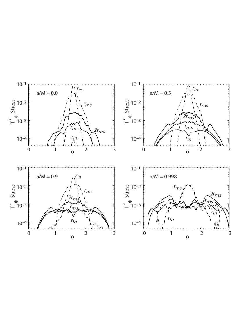
Figure 7: The azimuthally-averaged $T^{r}_{\phi}$ stress as a function of polar angle $\theta$, time-averaged over the last 75% of the simulation. The solid curves are the magnetic contribution to the outward-directed stress at $r=2r_{ms}$, $r=r_{ms}$ and the inner boundary. In the $a/M=0$ model the magnetic stress is inward-directed (dot-dashed line). The dashed lines are the mass contribution to the stress, (i.e., $\rho hU^{r}U_{\phi}$), at $r=r_{ms}$ and the inner boundary.

The plot for the Schwarzschild model is straightforward. The matter angular momentum flux narrows going from $2r_{ms}$ to $r_{ms}$, while the magnetic stress peaks through the disk and drops off through the corona. In the corona there is a region where the outward electromagnetic stress exceeds the inbound matter flux. There is negligible electromagnetic angular momentum flux at the inner boundary, and what there is is ingoing, represented by a dot-dashed line.

In contrast, all the non-zero spin simulations have a significant outward angular momentum flux carried by magnetic fields throughout the region between the marginally stable orbit and the inner boundary. Moreover, as was also shown in Figure  5, the magnitude of this flux relative to the stress associated directly with matter ($\rho hU^{r}U_{\phi}$, the dashed curve in the figure) increases steadily with increasing $a/M$. As $a/M$ increases, the angular width through which the magnetic angular momentum flux travels both spreads and develops a double-maximum structure. That is, when the black hole spins slowly, the magnetic angular momentum flux is largely confined to the region where the matter flux is greatest, a span of perhaps $\pm 30^{\circ}$ on either side of the equatorial plane. Moving from the disk to the corona, there is a point where the magnitude of the magnetic stress exceeds that of the matter stress. When the black hole spins rapidly, the magnetic angular momentum flux is relatively constant with polar angle through the disk region, but rises to a maximum at the funnel wall and slowly declines in the funnel interior toward the axis.

In the Schwarzschild simulation the magnetic stress peaks within the disk, and falls as the flow approaches the hole, becoming inward-directed at the inner boundary. In the $a/M=0.5$ simulation the magnetic stress can be described in terms of two pieces: a contribution spanning a broad angular range that increases slowly with increasing radius, and another contribution whose angular extent roughly matches that of the disk matter and grows toward larger radii. As the black hole spins faster, the relative importance of the broad angular range component grows, and a double-peak structure develops, with the greatest stress occurring near the funnel wall.

We can understand these trends in terms of a changing balance between effects arising from the magnetorotational instability in the disk and effects stemming from magnetic coupling to the spin of the black hole itself. In the disk, the stress results from MHD turbulence generated by the MRI (Balbus & Hawley 1998), and the magnetic stress is tied directly to the presence of the matter. The narrow disk component can be identified with this process; it increases with radius because its gradient must match that of $\dot{M}U_{\phi}$, which increases with radius. The broader component we associate with frame-dragging acting on the magnetic field in the corona and outflow. Close to the black hole, the magnetic field intensity varies little with angle, so there can be stress across a wide range of polar angles. Its magnitude changes little with radius because the matter density is so small in the corona and outflow that there can be little angular momentum exchange between fields and matter.

In rough terms, it is possible to separate the electromagnetic angular momentum flux going into the disk from that going into the corona by evaluating this flux on the shell at $r=r_{ms}$ and distinguishing disk from corona in terms of polar angle. Applying this criterion quantifies some of the remarks of the previous paragraphs: as $a/M$ increases, the ratio of the electromagnetic angular momentum flux entering the corona to that entering the disk rises from tiny ($<10^{-3}$ in the Schwarzschild case) to $\simeq 0.3$ ($a/M=0.5$), $\simeq 1$ ($a/M=0.9$) and $\simeq 3$ ($a/M=0.998$). Because angular momentum can readily move from matter to fields and back again, and because polar angle distribution at a fixed radius does not fully distinguish the ultimate end of the flux, these numbers are not entirely well-defined; nonetheless, they do express the qualitative point that the corona receives a growing proportion as the black hole spins faster.

When the black hole spins rapidly, the overall level of electromagnetic angular momentum flux is so high that, despite the growing share devoted to the corona, the portion going into the disk is large enough that it fundamentally alters the angular momentum budget of the accretion flow. It appears that in both the $a/M=0.9$ and $a/M=0.998$ simulations, the time-average magnetic torque adds to the matter’s angular momentum over a substantial radial range from near the hole to $r_{ms}$ and beyond (Fig. 5). As a result of this process, the accretion flow is retarded. In Paper I, we observed that in each simulation an inner torus is created in the region immediately outside $r_{ms}$, and that the prominence of this inner torus increases with increasing $a/M$. The electromagnetic stress driven by the spin of the black hole is the likely origin of this dependence on $a/M$. In the case of the $a/M=0.998$ simulation, magnetic torques are so strong that the mean of the local angular momentum can exceed the value associated with a circular orbit. For example, the density-weighted ratio of local angular momentum to the angular momentum of a circular orbit at that radius rises from $\simeq 0.95$ to $\simeq 1.05$ in the inner torus region (see also Fig. 13 of Paper I). The effective potential for the flow is then not as flat as expected in the marginally stable region, and inflow cannot occur as easily (see also Fig. 3).

4.4 Fluid frame stresses

It is also useful to look at the stresses in the fluid frame. The MHD turbulence is primarily due to local instabilities, so its physics is best analyzed in the local fluid frame. In addition, Novikov & Thorne (1973) showed that, if the disk is assumed to be time-steady, axisymmetric, and geometrically thin, the vertically-integrated stress in the fluid frame can be written in the physically-enlightening form

$$W^{r}_{\phi}(r)={\dot{M}\Omega\over 2\pi}R_{T}(r/M,a/M),$$ (11)

where the function $R_{T}$ encapsulates both relativistic corrections and the net angular momentum flux (the notation here follows Krolik 1999). The assumption that stress goes to zero at the marginally stable orbit means that $R_{T}(r)=0$ at all radii $r\leq r_{ms}$. In the Newtonian limit of large $r$, $R_{T}\rightarrow 1$. In this relation, “stress” means the part of the stress tensor other than that directly associated with accretion, i.e., $W^{r}_{\phi}=T^{r}_{\phi}-\dot{M}U_{\phi}(r)$, where $U_{\phi}(r)$ is the circular orbit angular momentum at $r$.

To compare our results with the Novikov-Thorne prediction, we compute a closely-related quantity,

$${\cal W}^{(r)}_{(\phi)}(r)\equiv{\int\,d\theta\,d\phi\,\sqrt{-g}\left[||b||^{2}U^{\mu}U_{\nu}-b^{\mu}b_{\nu}\right]\hat{e}_{\mu}^{(r)}\hat{e}^{\nu}_{(\phi)}\over\int\,d\phi\,\sqrt{-g(\theta=\pi/2)/g_{\theta\theta}(\theta=\pi/2)}},$$ (12)

where the $\hat{e}^{\mu}_{(\nu)}$ are an orthonormal tetrad designed to represent the directions labeled by $(\nu)$ in the fluid frame (see Appendix for details about their construction). We limit the integration to the bound portion of the flow, where $-hU_{t}<1$. We divide the shell-integrated fluid-frame stress by the area per unit radial coordinate in the equatorial plane in order to give this ${\cal W}^{(r)}_{(\phi)}$ the same units as $W^{r}_{\phi}$.

We compute ${\cal W}^{(r)}_{(\phi)}(r)$ at $t=8000\,M$ for all four simulations; this is shown in Figure 8. To facilitate comparison of simulations with different black hole spins, the value of ${\cal W}^{(r)}_{(\phi)}$ displayed in each panel is normalized to the initial maximum pressure found in that simulation. There is rough agreement with the Novikov-Thorne prediction (assuming the time-average accretion rate at the inner boundary) for $1.5r_{ms}\lesssim r\lesssim 40M$. At larger radii, one would not expect agreement because that is the region in which the matter in our simulations must move outward to absorb the angular momentum flux, whereas in the Novikov-Thorne model that region is supplied by accreting matter from farther away. Inside $r_{ms}$, however, where the Novikov-Thorne model predicts zero stress, our data are dramatically different. We find that the stress continues quite smoothly, and, in fact, continues to increase in amplitude from $r_{ms}$ to the inner boundary whenever $a/M>0$. Only in the Schwarzschild case does the fluid-frame stress eventually go to zero, albeit only very close to the event horizon.

In other words, there is considerable outward angular momentum flux in the fluid frame virtually throughout the flow, including the plunging region. Moreover, whenever $a/M>0$, there is always at least some outward angular momentum flux in the fluid frame even at the smallest radii outside the event horizon. Further, even with the overall normalization, the general level of the fluid-frame magnetic stress rises substantially with increasing $a/M$. This is due to the increasing amplitude of the magnetic fields. Thus, while there is a fluid-frame stress edge in the Schwarzschild case just outside the event horizon, there is no fluid-frame stress edge when the black hole spins.

 

 

Figure 8: The shell-integrated magnetic $r$-$\phi$ stress in the fluid frame per unit area in the equatorial plane is plotted against radius for each of the four simulations at a selected late time. The dashed curves show the prediction of the Novikov-Thorne model for the time-average accretion rate at $r_{in}$ for each of these simulations.

The standard Novikov-Thorne model assumes a cold, unmagnetized disk, with $h=||b||^{2}=0$. The origin of the stress is unspecified, although it is presumed due to turbulent motions. In our simulations neither $h$ nor $||b||^{2}$ is zero. In the calculation of Figure 8 we included only the magnetic stress and neglected the turbulent Reynolds stress, i.e., $\rho hU^{r}\delta U_{\phi}$, where the perturbation is with respect to a local circular orbit. Local simulations (Hawley, Balbus & Winters 1999) show that the Reynolds stress is generally a factor of several less than those due to the magnetic fields. Obviously the presence of magnetic fields explains the qualitatively different behavior of ${\cal W}^{(r)}_{(\phi)}$ and $W^{r}_{\phi}$ from the marginally stable region inward.

Another potential influence on the stress edge is the temperature in the disk and the associated vertical scale height. Purely hydrodynamical models of accretion disks more detailed than the Novikov-Thorne model (e.g., Muchotrzeb & Paczyński 1982; Matsumoto et al. 1984) relax the assumption of $h=0$ and consider the effects of finite geometric disk thickness. These studies indicate that, although the inner boundary for stress may not coincide exactly with the marginally stable orbit, in thin disks it should lie very close. Even in “slim disks” (Abramowicz et al. 1988), the stress does not extend all the way across the plunging region: in the pseudo-Newtonian approximation, designed to mock up Schwarzschild metric dynamics, the innermost radius for the end of stress stretches inward from $6M$ to $4M$ as the disk thickens. But it is clear that the purely hydrodynamic picture is inadequate; magnetic stresses operate in ways that Reynolds stresses and simple viscosity cannot. Further, in the MHD simulations there is significant magnetic field in the surrounding disk corona; the magnetic scale height is greater than the gas pressure scale height of the disk. In fact, the magnetic scale height near the black hole is $\sim r$ more or less independent of the matter scale height in the disk. Thus, when magnetic fields are included, the picture changes qualitatively from the purely hydrodynamic predictions.

Earlier we found that, when stress is measured in the coordinate frame, there is no stress edge anywhere. When it is evaluated in the fluid frame, the situation changes only slightly: when $a/M>0$, there is similarly no stress edge; when $a/M=0$, one exists, but it is deep in the plunging region, immediately outside the event horizon.

5 Energy transport

5.1 Energy fluxes

The conventional approach to defining the radiative efficiency of accretion onto black holes was set out by Novikov & Thorne (1973). In the standard picture, thermal energy in the disk is assumed negligible compared to orbital energy, in part because the thermal loss time is assumed to be very short compared to the inflow time everywhere outside $r_{ms}$. With those assumptions, the radiation rate in each ring is simply the difference between the energy brought into that ring by mechanical work (torques acting on the ring by neighboring zones) and energy lost from that ring by accretion. Both contributions amount, of course, to the radial divergence of an energy flux which does not vanish; the energy deposited by the flux is the disk’s luminosity. As the fluid drops toward the hole, it becomes increasingly bound, with a binding energy equal to that of the circular orbit at its radius. The energy of the last circular orbit at $r_{ms}$ sets the canonical efficiency of standard thin disk accretion, $\eta=1+U_{t}(r_{ms})$. For a Schwarzschild hole this is $0.057$.

In the simulations, things are less straightforward. As in the standard picture, energy is extracted from orbital motion as the gas accretes, but that energy is not radiated. It first goes into magnetic fields and velocity fluctuations within the turbulent disk. Some magnetic field rises out of the disk into the corona, and a general coronal outflow removes some energy from the disk. As the turbulence in the disk is dissipated at the grid scale, some of the energy is converted into heat by artificial viscosity; some is lost. Enough of this energy is retained to keep the disk hot.

We can investigate how energy is transported in these simulations by considering the magnitude of the energy flux, given by the $T^{r}_{t}$ component of the stress tensor. Just as for the angular momentum flux, it has both a fluid part

$$\left(T^{r}_{t}\right)_{\rm fluid}=\rho hU^{r}U_{t}$$ (13)

and an electromagnetic part

$$\left(T^{r}_{t}\right)_{\rm EM} = ||b||^{2}U^{r}U_{t}-b^{r}b_{t}$$ (14)

$$= F^{\mu r}F_{\mu t}$$

$$= g^{rr}\left(g^{\phi\phi}{\cal E}^{\phi}{\cal B}^{\theta}-g^{\theta\theta}{\cal E}^{\theta}{\cal B}^{\phi}-g^{t\phi}{\cal E}^{r}{\cal E}^{\phi}\right),$$

where ${\cal E}^{r}=V^{\phi}{\cal B}^{\theta}-V^{\theta}{\cal B}^{\phi}$, ${\cal E}^{\theta}=V^{r}{\cal B}^{\phi}-V^{\phi}{\cal B}^{r}$, and ${\cal E}^{\phi}=V^{\theta}{\cal B}^{r}-V^{r}{\cal B}^{\theta}$. The last form for the electromagnetic energy flux shows that it is the radial component of the Poynting flux, modified by a frame-dragging correction.

In a steady-state disk, $T^{r}_{t}$ integrated over spherical shells should be constant with radius. However, because its largest contribution is from the flow of rest-mass, its radial behavior is dominated by that flux, a conserved quantity to which we have already devoted much attention (§3.1). In order to focus attention on the non-rest-mass portion, we instead study shell-integrals of time-averaged $T^{r}_{t}-\dot{M}=\langle\langle\rho(hU_{t}+1)U^{r}+||b||^{2}U^{r}U_{t}-b^{r}b_{t}\rangle\rangle$. In a time-steady disk, the constancy of $\dot{M}$ with radius means that this “adjusted” energy flux should likewise be constant as a function of $r$. In an effort to make still closer contact with ordinary intuition, in Figure 9 we plot $1-\langle\langle T^{r}_{t}\rangle\rangle/\langle\dot{M}\rangle$, the binding energy per unit rest-mass accreted, but restricting the integral to cells in which the matter is bound. In this figure, the dashed line is the specific energy carried by the fluid term alone (eq. 13), and the solid line is obtained from both the fluid and electromagnetic components. As references, there are two dotted lines: the straight one shows the binding energy of the marginally stable orbit, the curved one the binding energy of a circular orbit in the equatorial plane at that radius.

Figure 9: Specific energy flux, defined as $1-\langle\langle T^{r}_{t}\rangle\rangle/\langle\dot{M}\rangle$ for each of the four simulations. The dashed line is derived using the fluid energy flux only, while the solid line has both the fluid and electromagnetic energy flux. The dotted line corresponds to the specific energy of a circular orbit at each radius; the horizontal dotted line is the specific energy of the marginally stable circular orbit at at $r_{ms}$.

If all the simulations achieved a steady state within the region shown, and if there were no energy exchange between bound matter and anything else, the solid line would be flat. As is immediately apparent, it is not. At large radii, the fluid binding energy flux (dashed line) closely tracks the orbital energy curve. This is because the numerical energy loss time is shorter than the inflow time, crudely mimicking the effects of radiation losses in a real accretion disk. At smaller radii, the fluid binding energy is smaller than the orbital binding energy for two reasons: artificial viscosity adds heat to the gas, and the inflow time becomes shorter than the numerical loss time. Some energy is lost to the outflow, especially when $a/M\geq 0.9$, but not enough to strongly cool the disk. Here the mimicry is closer in spirit to a non-radiative disk.

5.2 Poynting flux

Figure 10: Time- and azimuthally-averaged outgoing Poynting flux in the four simulations, plotted on the same linear scale. The values are normalized by the initial energy and multiplied by $10^{4}$. As the black hole spins more rapidly, the Poynting flux associated with the funnel-wall outflow rapidly grows in importance.

At all radii there is a substantial offset between the total energy flux curve and the fluid-only curve. This offset is due to the outward energy flux conveyed electromagnetically (Fig. 10). With the exception of the inner boundary in the zero-spin simulation (where it is also very small in magnitude), the Poynting flux is always directed outward. Independent of the black hole spin, there is always Poynting flux associated with the work done by torques in the disk. In the outer portions of the accreting disk ($r\simeq 15M$), where our initial conditions make all four simulations very similar, its magnitude varies little with black hole spin. However, in the inner disk, where the mean magnetic field strength grows substantially with more rapid rotation, so does the Poynting flux. At the equator on the inner boundary, it increases by about a factor of two from $a/M=0.5$ to $a/M=0.9$ and by almost an order of magnitude from $a/M=0.9$ to $a/M=0.998$.

Poynting flux in the jet outflow varies far more dramatically with black hole spin. It is negligible in the Schwarzschild simulation, while in the $a/M=0.998$ simulation the Poynting flux in the funnel wall completely dominates the Poynting flux in the disk. Another way to make this comparison is to consider the ratio of the total (outward) shell-integrated Poynting flux to the (inward) fluid energy flux (nearly all rest-mass energy). This ratio is plotted in Figure 11. Here we see that relative to the rate at which fluid energy is accreted, the Poynting flux integrated over the inner boundary rises from 0.25% when $a/M=0.5$ to $\sim 1$% when $a/M=0.9$ to $\sim 10$% when $a/M=0.998$. These ratios increase steadily outward for the $a/M=0$ and $0.5$ simulations, and have a local maximum around $r=3$–$5\,M$ for the high spin models. In the simulation with the most rapid spin at the radius where this ratio reaches its maximum, Poynting flux carries outward $\sim 60$% of the ingoing fluid energy flux.

Figure 11: Ratio of time-averaged electromagnetic energy flux, $\langle\langle T^{r}_{t}\rangle\rangle_{EM}$ to fluid energy flux, $\langle\langle T^{r}_{t}\rangle\rangle_{fluid}$, as a function of radius. The solid line corresponds to the $a/M=0.0$ run, the dotted line to $a/M=0.5$, the dashed line to $a/M=0.9$ and the dot-dashed line to $a/M=0.998$. As the spin of the black hole increases, an increasing fraction of the energy flux is in the form of Poynting flux.

Another way to look at these results is from the point of view of the Penrose process. In its simplest form, this process depends on the fact that inside ergospheres there can exist negative energy orbits, so that black holes can give up energy (i.e., lose mass) by absorbing particles with negative energy. An analogous process exists for magnetic fields. The electromagnetic “energy density at infinity” may be defined (Koide 2003) by

$$e_{\rm EM}^{\infty}/\alpha=-T^{t}_{t}(EM)=- (1/2)g^{tt}\left[g^{rr}({\cal E}^{r})^{2}+g^{\theta\theta}({\cal E}^{\theta})^{2}+g^{\phi\phi}({\cal E}^{\phi})^{2}\right]+(1/2)\left(g^{t\phi}{\cal E}^{\phi}\right)^{2}$$ (15)

$$+\left[g^{\theta\theta}g^{\phi\phi}({\cal B}^{r})^{2}+g^{rr}g^{\phi\phi}({\cal B}^{\theta})^{2}+g^{rr}g^{\theta\theta}({\cal B}^{\phi})^{2}\right].$$

¿From this form we see that, if all the spatial elements of the inverse metric were positive definite, $e_{\rm EM}^{\infty}$ could never be negative. However, inside the ergosphere, $g^{\phi\phi}<0$. Thus, negative electromagnetic energy-at-infinity is associated with regions inside the ergosphere where the components of the field tensor associated with poloidal magnetic field (${\cal B}^{r}$ and ${\cal B}^{\theta}$) and toroidal electric field (${\cal E}^{\phi}$) are large in magnitude compared to the other field components. Moreover, because ${\cal E}^{\phi}=V^{\theta}{\cal B}^{r}-V^{r}{\cal B}^{\theta}$, a large poloidal magnetic field also helps to make ${\cal E}^{\phi}$ large, particularly when the poloidal transport speed is substantial. That an electromagnetic version of the Penrose process is at work is suggested by the fact that in the $a/M=0.9$ and 0.998 simulations, the time-averaged $e_{\rm EM}^{\infty}<0$ in the region within $40^{\circ}$ – $60^{\circ}$ of the equatorial plane and $\simeq 0.3M$ of the inner boundary.

One of the key questions of black hole accretion is whether or not energy can be extracted from the region inside $r_{ms}$. Although it is difficult to say how much radiation will escape from inflowing gas within the plunging region (discussed below), it is clear that the Poynting flux provides an avenue for the outward transport of energy from the plunging region and from the black hole itself.

5.3 Radiation

Although the present simulations do not include radiative losses, it is interesting nevertheless to consider whether the standard assumptions of thin disk theory would apply. The issues involve where and how rapidly energy is dissipated into heat, and whether there is sufficient time for the heat to be transformed into photons and radiated prior to the gas entering the black hole. Well outside the marginally stable orbit, the time required for these processes to occur should be significantly shorter than the inflow time. Where that is true, the conservation law approach to computing the radiation rate should work well. In the simulations the turbulent energy released by dissipation is captured only partially by artificial viscosity; numerical losses thus mimic radiation losses, and in most of the main disk body, the numerical loss time is appropriately shorter than $t_{in}$. The only difference between the simulations and the Novikov-Thorne model in this regard is that we do not force the stress to go to zero at $r_{ms}$. A formalism for tracing the consequences of that changed boundary condition in time-steady disks was developed in Agol & Krolik (2000). Applying it to the simulation results indicates an enhanced radiative efficiency from this part of the disk that is relatively modest for the cases with $a/M=0$, 0.5, and 0.9. Because the $a/M=0.998$ simulation did not achieve an inflow steady-state, the assumptions of this formalism may not be valid, but the data suggest that the enhancement to the radiative efficiency may be considerably larger.

Inside $\simeq 2r_{ms}$, the inflow time falls rapidly (see Fig. 3), becoming roughly an orbital period near and inside $r_{ms}$. It then becomes questionable whether the several processes that stand between inter-ring work and radiation have enough time to run to completion. If not, the gas advects its energy inward, much as envisioned by Rees et al. (1982), Narayan & Yi (1995), and Abramowicz et al. (1988), albeit for different reasons. However, particularly in the plunging region proper, new processes can lead to radiation. Machida & Matsumoto (2003) suggest that field reconnection in the plunging region could lead to X-ray flares. Rather than magnetic field being dissipated on very small lengthscales at the end of a turbulent cascade, it can instead by dissipated in large-scale current sheets. In Hirose et al. (2004) we drew attention to the prevalence of high current density regions in the inner disk and plunging region where the current density is so high that rapid field dissipation might be expected. If the local temperature in these current sheets can be raised high enough that Compton scattering is the dominant cooling mechanism, radiation can release energy very rapidly: the Compton cooling time is

$$t_{C}={3\over 4}{m_{e}\over\mu_{e}}\left({L\over L_{E}}\right)^{-1}\left({r\over M}\right)^{3}M,$$ (17)

where $\mu_{e}\sim m_{p}$ is the mass per electron and $L$ is the luminosity of seed photons injected within radius $r$. Some of these photons will be captured by the black hole, and some will strike the disk farther out, but some portion will also reach distant observers. To compute the actual radiative efficiency of flows of this sort will require calculations that explicitly balance the various competing processes and timescales.

6 Discussion and Summary

In Paper I of this series we reported that the fraction of the initial mass accreted in a fixed time diminishes sharply with increasing black hole spin. We also noted that the angular momentum per unit rest-mass that is accreted likewise drops as the black hole spins more rapidly, and by significantly more than the associated decrease in the specific angular momentum of the innermost stable circular orbit. On the basis of the more detailed analysis presented here, we can now explain both these effects. Not surprisingly, they are closely related.

An examination of the angular momentum fluxes in the accretion flow reveals how significant magnetic fields are to the evolution of the inner region of a black hole accretion disk. The low $a/M$ models attain a quasi-steady state that behaves much as one would expect from simple accretion disk theory. The net flux of angular momentum through the disk is essentially equal to the value carried into the black hole. Within the flow itself outward-going magnetic angular momentum flux balances the excess in the inward-going component carried by the matter flow.

Contrary to standard accretion theory, however, there are always magnetic stresses exerted across the location of the marginally stable orbit and in the plunging region interior to this point. In fact, when the black hole rotates, the $r$–$\phi$ component of the stress tensor in the fluid frame rises more steeply with decreasing radius in the plunging region than in the disk itself. Thus, we have shown that the concerns voiced quietly in Page & Thorne (1974) and Thorne (1974) have been borne out: the presence of magnetic fields invalidates the “zero-stress” inner boundary condition.

Hirose et al. (2004) showed that the relative magnitude of the magnetic field in the inner disk grows steadily with increasing black hole spin. This is a by-product of the creation of the dense inner torus: higher pressure gas can support stronger magnetic field when the field’s origin lies in the magneto-rotational instability. Thus, as the spin increases, the magnetic stresses grow rapidly stronger. There is more going on than can be attributed merely to stronger field strengths, however. The rotating hole itself represents a source of angular momentum and energy that can be carried outward by the magnetic stress. When $a/M\gtrsim 0.9$, the magnetic stresses carry out of the ergosphere an angular momentum flux that is comparable to what is brought inward with accreting matter. A striking suppression of the accretion rate is the result. In the most extreme case ($a/M=0.998$), accretion through the inner disk is retarded to such a degree that even in a simulation time of $8100\,M$ no accretion equilibrium is achieved; rather, the mass of the inner torus builds steadily through the simulation as matter accretes from outside, but is held back not far outside $r_{ms}$. This result is reminiscent of the suggestion by van Putten and Ostriker (2001) that magnetic torques driven by rotating black holes might lead to a state of suspended accretion, but the field structure we see (turbulent field, largely confined to the accreting matter) is quite different from the one posited by them (organized poloidal field with loops spanning all the way from the disk to the event horizon).

We should note that although the accretion rate over the course of our simulation is reduced by a factor of 4 contrasting the simulation with $a/M=0.998$ to the one with $a/M=0$, the evident lack of equilibrium in the former case prevents us from saying what will happen in the long run. It is possible that when the inner torus mass grows large enough, the time-averaged accretion rate will rise. In that case, the effect of black hole spin would be better described as altering the relation between accretion and inner disk mass rather than as a simple suppression of accretion. On the other hand, without doing more extended simulations, we cannot say whether such an equilibrium is ever achieved—it is possible that the structure of the inner disk traverses some complicated limit cycle when the black hole spins very rapidly. In any case, it is clear that a magnetized spinning black hole can affect the rate at which matter accretes into it in ways that go beyond the changes in the effective potential usually considered.

Another consequence of the substantial magnetic torques near the black hole is a reduction in the net angular momentum brought to the hole as a result of accretion. As mentioned briefly in Paper I and at greater length in Gammie et al. (2004), the accreted angular momentum per unit rest-mass decreases so much with increasing $a/M$ that the black hole can spin down (in the sense of decreasing $a/M$) even as $M$ increases. Our results are in approximate agreement with those of Gammie et al. in indicating that there is near balance when $a/M\approx 0.9$, but likely net spin-down for greater $a/M$. This result suggests that black holes cannot be spun-up by accretion to $a/M\gtrsim 0.9$; only a black hole merger might create a more rapidly spinning black hole.

We also examined energy transport in the vicinity of the black hole. As with angular momentum transport, the combination of magnetic fields and rotating holes leads to phenomena not normally included in standard disk theory. Magnetic fields can extract both energy and angular momentum from the black hole in a fashion resembling the Blandford & Znajek (1977) mechanism, but with several notable differences. First, the magnetic field is far from force-free. Second, the relevant field lines connect the plunging region to the disk and the outflow rather than only connecting the event horizon to infinity (cf. similar results found by McKinney & Gammie 2004). Energy is drawn from a rotating black hole in a manner that, far from being independent of accretion as in the original Blandford-Znajek picture, is inherently dependent upon accretion. In fact, the most convenient way to describe its magnitude is relative to the rate at which rest-mass is accreted: for modest spins, the electromagnetic energy release per unit mass is $\lesssim 1\%$, while for very rapid spin, it can be $\simeq 10\%$ or more. As the spin increases, the angular distribution of the Poynting flux also changes, with most going into the disk at low spin but the greater share entering the outflow when the black hole spins very rapidly.

The simulations have demonstrated several new dynamical effects for magnetically driven accretion flows in a Kerr metric. At this point we can give only qualitative assessment of the observational consequences of these effects. For example, strong outward magnetic angular momentum flux from a spinning black hole leads to a substantial alteration in the mass surface density distribution, creating a sizable inner torus in the region just outside $r_{ms}$. Completely unexpected in conventional disk models, this large mass concentration could significantly alter the expected X-ray reflectivity of this region deep in the relativistic potential. Because magnetic stresses continue throughout the inner disk and plunging region, the efficiency with which orbital shear energy can be dissipated into heat and then escaping photons could be greater than conventionally envisioned, but quantitative results require an improved treatment of thermodynamics. For rapidly spinning holes, the Poynting flux represents a very significant part of the energy flow near the black hole. Although the impact of these effects on disk thermal emission remains to be worked out, their presence will surely lead to significant effects not found in traditional models.

Appendix A Defining the Fluid Frame Tetrads

In order to compute quantities measured by a physical observer, one must define a set of basis vectors (commonly called “tetrads”) appropriate to that observer, which we write here as $\hat{e}^{\mu}_{(\nu)}$ for the contravariant set. In this notation, $(\nu)$ identifies the direction in the observer’s frame.

Ideally, these should be directed in four-space so as to be most useful for physical interpretation. For example, in most instances it is important to be able to identify the direction of proper time in the observer’s frame. This is simply done by setting $\hat{e}^{\mu}_{(t)}=U^{\mu}$, the observer’s four-velocity. In the observer’s own frame, the only non-zero component of the four-vector is the time component, so it automatically satisfies the requirement of appropriate directionality. Because $U^{\mu}U_{\mu}\equiv-1$, it is also automatically normalized to unit magnitude.

Identifying other directions is, in general, more ambiguous. One can always construct the remaining three tetrads by a Gram-Schmidt procedure, requiring the newly-constructed tetrad element to be orthogonal to all the previously-defined ones and normalized to unit magnitude. However, there are many different ways in which the tetrad elements can be ordered for this procedure and the results depend on the ordering. In fact, the results depend in general on whether one first seeks contravariant or covariant versions. This mathematical ambiguity emphasizes the physical ambiguity in identifying spatial directions in one frame with those in another.

For our purposes, we wish to construct a tetrad basis set that both reduces to the conventional directions in the Newtonian limit and may be most directly compared with the set chosen by Novikov & Thorne (1973). The choice made by Novikov and Thorne is a special case that is unambiguous because they were interested only in the limit that $U^{r}=U^{z}=0$ in the coordinate frame. When that is so, tetrad elements that are purely radial or purely vertical in the coordinate frame are automatically orthogonal to the four-velocity. Consequently, the $R$ and $z$ tetrad elements can be taken as purely radial and vertical in the coordinate frame, while the $t$ and $\phi$ elements couple only to each other. This so simplifies the problem that no ambiguities remain.

Although the components of the fluid four-velocities found in our simulations are in general non-zero everywhere, in much of the simulation region, $U^{\phi}\gg U^{r},U^{\theta}$. In an effort to ensure that the direction of greatest difference between the fluid frame and the coordinate frame is aligned as closely as possible, after setting $\hat{e}^{\mu}_{(t)}=U^{\mu}$, we begin the Gram-Schmidt process with the $\phi$ element of the tetrad and set its $r$- and $\theta$-components in the coordinate frame to zero everywhere. The $r$-element can then be constructed with a zero $\theta$-component, but it is also necessary to insist that $\hat{e}^{r}_{(r)}>0$ to preserve the right orientation of the tetrad set. Finally, only the $\theta$-element remains to be computed; it has non-zero components in all four coordinates. The result is:

$$e_{(t)}^{\mu} = \left[U^{t},U^{r},U^{\phi},U^{\theta}\right]$$ (A1)

$$e_{(r)}^{\mu} = (s/N_{2})\left[-g^{tt}C_{1}-g^{t\phi}C_{2},G^{rr}C_{0},-g^{\phi\phi}C_{2}-g^{t\phi}C_{1},0\right]$$ (A2)

$$e_{(\phi)}^{\mu} = -(1/N_{1})\left[l,0,1,0\right]$$ (A3)

$$e_{(\theta)}^{\mu} = (1/N_{3})\left[1,(C_{1}/C_{0})(g^{tt}-l^{2})/g^{rr},-l,\right.$$ (A4)

$$\left.C_{-}/C_{3}-(U^{r}/U^{\theta})(C_{1}/C_{0})(g^{tt}-l^{2})/g^{rr}\right],$$

where

$$l \equiv U_{\phi}/U_{t}$$

$$C_{0} \equiv U^{t}U_{t}+U^{\phi}U_{\phi}$$

$$C_{1} \equiv U^{r}U_{t}$$

$$C_{2} \equiv U^{r}U_{\phi}$$

$$C_{3} \equiv U^{\theta}U_{t}$$

$$C_{-} \equiv U^{\phi}U_{\phi}-U^{t}U_{t}$$

$$N_{1} \equiv \left(g_{tt}j^{2}-2g_{t\phi}j+g_{\phi\phi}\right)^{1/2}$$

$$N_{2} \equiv \left(g^{tt}C_{1}^{2}+g^{rr}C_{0}^{2}+g^{\phi\phi}C_{2}^{2}+2g^{t\phi}C_{1}C_{2}\right)^{1/2}$$

$$N_{3} \equiv \left[g^{tt}-2g^{t\phi}j+(C_{1}/C_{0})^{2}(g^{tt}-j^{2})^{2}/g^{rr}\right.$$

$$+\left.g^{\phi\phi}j^{2}+g^{\theta\theta}(C_{-}/C_{3}-(U^{r}/U^{\theta})(C_{1}/C_{0})(g^{tt}-j^{2})/g^{rr})^{2}\right]^{1/2}$$

$$s \equiv C_{0}/|C_{0}|.$$

References

- Abramowicz et al. (1988) Abramowicz, M., Czerny, B., Lasota, J.-P. & Szuszkiewicz, E. 1988, ApJ, 332, 646
- Agol & Krolik (2000) Agol, E., & Krolik, J. H. 2000, ApJ, 507, 304
- Balbus & Hawley (1998) Balbus, S. A., & Hawley, J. F. 1998, Rev. Mod. Phys., 70, 1
- Blandford & Znajek (1976) Blandford, R. D. & Znajek, R. 1977, MNRAS 179, 433
- De Villiers, & Hawley (2003) De Villiers, J. P. & Hawley, J. F. 2003, ApJ, 589, 458
- De Villiers et al. (2003) De Villiers, J. P., Hawley, J. F. & Krolik, J. H. 2003, ApJ, 599, 1238 (Paper I)
- De Villiers et al. (2004) De Villiers, J. P., Hawley, J. F. Krolik, J. H. & Hirose, S., 2004, astro-ph/0407092, ApJ, submitted
- Gammie et al. (2004) Gammie, C. F., Shapiro, S. L. & McKinney, J. C. 2004, ApJ 602, 312
- Hawley, Balbus, & Winters (1999) Hawley, J. F., Balbus, S. A., & Winters, W. F. 1999, ApJ, 518, 394
- Hirose et al. (2004) Hirose, S., Krolik, J. H., Hawley, J. F., & De Villiers, J.-P. 2004, ApJ, 606, 1083
- Koide (2003) Koide, S. 2003, Phys. Rev. D., 67, 104010
- Krolik (1999) Krolik, J. H. 1999, Active Galactic Nuclei (Princeton: Princeton Univ. Press)
- Krolik & Hawley (2002) Krolik, J. H. & Hawley, J. F. 2002, ApJ, 573, 754
- Machida & Matsumoto (2003) Machida, M., & Matsumoto, R. 2003, ApJ, 585, 429
- Matsumoto et al. (1984) Matsumoto, R., Kato, S., Fukue, J. & Okazaki, A.T. 1984, PASJ, 36, 71
- McKinney & Gammie (2004) McKinney, J. C. & Gammie, C. F. 2004, ApJ, in press
- Muchotrzeb & Paczyński (1982) Muchotrzeb, B. & Paczyński, B. 1982, Acta Astron., 32, 1
- Narayan & Yi (1995) Narayan, R. & Yi, I. 1995, ApJ 444, 231
- Novikov & Thorne (1973) Novikov, I.D. & Thorne, K.S. 1973, in Black Holes: Les Astres Occlus, eds. C. de Witt & B. de Witt (New York: Gordon & Breach), 344
- Page & Thorne (1974) Page, D. N. & Thorne, K. S. 1974, ApJ, 191, 499
- Rees et al. (1982) Rees, M.J., Phinney, E.S., Begelman, M.C. & Blandford, R.D. 1982, Nature 295, 17
- Shakura & Sunyaev (1973) Shakura, N. I., & Sunyaev, R. A. 1973, A&A, 24, 337
- Thorne (1974) Thorne, K. S. 1974, ApJ, 191, 507
- van Putten & Ostriker (2001) van Putten, M. & Ostriker, E. C. 2001, ApJL, 552, 31L