21 cm Tomography of the High-Redshift Universe with the Square Kilometer Array

Abstract

We discuss the prospects for “tomography” of the intergalactic medium (IGM) at high redshifts using the 21 cm transition of neutral hydrogen. Existing observational constraints on the epoch of reionization imply a complex ionization history that may require multiple generations of sources. The 21 cm transition provides a unique tool to probe this era in detail, because it does not suffer from saturation effects, retains full redshift information, and directly probes the IGM gas. Observations in the redshifted 21cm line will allow one to study the history and morphology of reionization in detail. Depending on the characteristics of the first sources, they may also allow us to probe the era before reionization, when the first structures and luminous sources were forming. The construction of high signal-to-noise ratio maps on arcminute scales will require approximately one square kilometer of collecting area.

1 Introduction

One of the major goals of modern cosmology is to understand how the first luminous sources in the universe formed and grew into the galaxies and galaxy clusters that we see today. As technology has improved in the past four decades, the frontiers of our knowledge have extended farther and farther into the past. We now sit at the cusp of exploring the era in which the first generations of sources were just beginning to form: the end of the cosmological “dark ages.” Observations of this epoch will teach us about the transformation from the smooth, relatively simple universe that we see in the cosmic microwave background (CMB) to the complex universe that we see nearby.

The hallmark of the era of first objects is the “reionization” of the intergalactic medium (IGM), when these first luminous sources ionized the gas around them and rendered it transparent to ultra-violet photons that we observe today as optical or infrared light (see [2] and references therein). Fortunately, radio photons, including those from the CMB, readily propagate through both the neutral and ionized IGM at this time, and these will help us to measure an enormous amount of information about the process of reionization, the properties of the first sources, and the properties of the IGM [50, 6, 24].

Existing techniques have provided tantalizing constraints on the epoch of reionization (EOR). The most straightforward method is to observe the high redshift part of the “Ly$\alpha$ forest:” regions with relatively large HI densities appear as absorption troughs in quasar spectra, which presumably deepen and come to dominate the spectra as we approach the reionization epoch. Indeed, spectra of $z\sim 6$ quasars selected from the Sloan Digital Sky Survey (SDSS) show at least one extended region of zero transmission [3], indicating that the ionizing background is rising rapidly at this time [13] (but see [45]). However, the mean optical depth of the IGM to Ly$\alpha$ absorption is $\tau_{Ly\alpha}\approx 6.45\times 10^{5}{x_{H}}[(1+z)/10]^{3/2}$ [23], where ${{\bar{x}}_{H}}$ is the global neutral fraction. Even a modest ${{\bar{x}}_{H}}>10^{-3}$ will therefore render the absorption trough completely black; quasar absorption spectra can clearly probe only the latest stages of reionization.

A second constraint comes from the effects of the ionized gas on the CMB. The free electrons Thomson scatter CMB photons, washing out the intrinsic anisotropies but generating a faint polarization signal. The total scattering optical depth $\tau_{\rm es}$ is proportional to the column density of ionized hydrogen, so it provides an integral constraint on the reionization history. Recently, the Wilkinson Microwave Anisotropy Probe (WMAP) used the polarization signal to measure a large $\tau_{\rm es}$, indicating that reionization began at $z>14$ [28, 46]. A third (possibly conficting) constraint comes from measurements of the temperature of the Ly$\alpha$ forest at $z\sim 2$–$4$, which, taken at face value, require reheating of the IGM at $z<10$. Since heating is accomplished through photoionization, this would suggest an order unity change in the ionized fraction at $z<10$ [47, 26], though with large uncertainties.

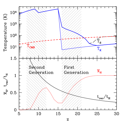
Taken together, these three sets of observations imply a complex reionization history extending over a large redshift interval ($\Delta z\sim 10$). This is inconsistent with a “generic” picture of fast reionization (e.g., [2], and references therein). The results seem to indicate strong evolution in the sources responsible for reionization, and a detailed measurement of the reionization history would contain a rich set of information about early structure formation [44, 50, 6, 24]. In fact, it is quite plausible that the ionization history is complex, with long periods of “stalling” or even two distinct epochs of reionization. Figure 1 illustrates why. Here we consider the possibility of two generations of ionizing sources [50, 6]. In the bottom panel we show the ratio of the recombination time (assuming the mean cosmic density and $T=10^{4}\mbox{ K}$, typical of ionized gas) to the age of the universe (solid curve). Note that the ratio is near unity at $z\sim 10$ and decreases at earlier times, implying that a significant fraction of the gas can recombine if it is ionized by this point. The dotted curve shows how ${{\bar{x}}_{H}}$ could evolve and roughly satisfy the three observational constraints. The first generation of sources (for example, very massive metal-free stars) ionize most of the gas. However, these sources quickly cease forming (perhaps because they enrich their environs with heavy elements) and most of the gas recombines. Full reionization must await the second generation of sources (in our example, Population II stars). We see from the Figure that the 21 cm structures could be long-lived and complex: for example, gas above the mean density may recombine between the two generations while voids remain ionized. The top panel illustrates the temperature evolution of the IGM in this scenario; note that reionization corresponds to a sudden boost in the temperature. This panel will be discussed in more detail below.

Figure 1: A cartoon illustrating a double reionization history. The bottom panel shows the ratio of the recombination time and the age of the universe (solid curve) as well as ${{\bar{x}}_{H}}$ (dotted curve). The top panel shows the kinetic temperature of the IGM gas (solid lines), the CMB temperature (short-dashed line), and the spin temperature (long-dashed line, note that for $z<23$ we assume this traces $T_{K}$). The thick solid line neglect all heating mechanisms except for photoionization, while the thin line shows what could happen if X-ray and shock heating were included (see §3). The shaded regions mark the two generations of ionizing sources.

While such cartoon views are certainly plausible, detailed models rely on a number of uncertain parameters that we would like to measure. The optimal reionization experiment would: (1) be sensitive to order unity changes in ${{\bar{x}}_{H}}$ (to probe the crucial middle stages of reionization), (2) provide measurements that are well-localized along the line of sight (rather than a single integral constraint), and (3) not require the presence of bright background sources, which may be rare at high redshifts. The most promising candidate proposed to date is the 21 cm hyperfine transition of neutral hydrogen in the IGM [14, 15], which fulfills all three of these criteria.

So long as the excitation temperature $T_{S}$ of the 21 cm transition in a region of the IGM differs from the CMB temperature, that region will appear in either emission (if $T_{S}>T_{\rm CMB}$) or absorption (if $T_{S}<T_{\rm CMB}$) when viewed against the CMB. Variations in the density of neutral hydrogen (due either to large-scale structure or to HII regions) would appear as fluctuations in the sky brightness of this transition. Because it is a line transition, the fluctuations can also be well-localized in redshift space. Thus, in principle, high resolution observations of the 21 cm transition in both frequency and angle can provide a three-dimensional map of reionization. Together with radio absorption spectra of bright background sources (see the contribution by Carilli, this volume), these observations promise to shed light both on the early growth of structure and on reionization.

In the following, we will distinguish two observational goals. The ultimate goal is to make three-dimensional, high signal-to-noise maps of the sky in the 21 cm transition. In addition to precisely mapping reionization itself, this would, for example, allow detailed comparisons between the distribution of neutral gas and the ionizing sources. Unfortunately, we will find below that the expected brightness of the IGM is extremely small both in absolute terms and when compared to the relevant foreground contaminants. It is therefore considerably easier to make statistical measurements of the distribution of neutral gas. As we have seen with CMB measurements, these statistical constraints can be quite powerful.

In §2 we will briefly review the important physics of the 21 cm transition. In §3 we will outline the information we can expect to learn from 21 cm observations, and in §4 we will describe the instrumental requirements for making maps and statistical measurements. Finally, in §5 we conclude and discuss 21 cm observations in relation to other instruments that will be built in the next decade.

2 The 21 cm Transition

We define $\delta T(\nu)$ to be the observed brightness temperature increment between a patch of the IGM, at a frequency $\nu$ corresponding to a redshift $1+z=\nu_{0}/\nu$ (where $\nu_{0}=1420.4\mbox{ MHz}$ is the rest frequency of the 21 cm transition), and the CMB. Assuming the WMAP cosmological parameters [46] and small 21 cm optical depth $\tau_{21}<<1$, this quantity is [42, 33]:

$$\delta T(\nu) \approx \frac{T_{S}-T_{\rm CMB}}{1+z}\,\tau_{21}$$ (1)

$$\approx\, 23\,(1+\delta){x_{H}}{\mathcal{T}}\left(\frac{1+z}{10}\right)^{1/2}\mbox{ mK},$$

where ${\mathcal{T}}=(T_{S}-T_{\rm CMB})/T_{S}$, $T_{S}$ is the spin temperature of the IGM, ${x_{H}}$ is the neutral fraction, and $\delta$ is the overdensity. All of these local quantities should be averaged over the volume sampled by the telescope beam (note that we will use ${{\bar{x}}_{H}}$ for the global, mass-averaged neutral fraction). For reference, one arcminute subtends $\approx 1.9h^{-1}$ comoving Mpc at $z=10$ in the WMAP cosmology, while a bandwidth of $0.1\mbox{ MHz}$ corresponds to $\approx 1.7\mbox{ Mpc}$ at the same redshift.

The observability of the IGM clearly depends on the spin temperature, which may be written [14, 15]:

$$T_{S}=\frac{T_{\rm CMB}+y_{c}T_{K}+y_{{\rm Ly}\alpha}T_{{\rm Ly}\alpha}}{1+y_{c}+y_{{\rm Ly}\alpha}}.$$ (2)

The second term describes collisional excitation of the hyperfine transition, which couples $T_{S}$ to the gas kinetic temperature $T_{K}$. The coupling coefficient $y_{c}\propto n_{H}$ has been numerically evaluated by [1]; it becomes strong when $1+\delta>5[(1+z)/20]^{2}$ and is not important in the smooth IGM in the relevant redshift range. The third term in equation (2) describes the Wouthuysen-Field effect, in which Ly$\alpha$ pumping couples the spin temperature to the color temperature of the radiation field $T_{{\rm Ly}\alpha}$ [49, 14] (which equals $T_{K}$ in most astrophysical environments [16]). The physics of this mechanism have been described recently in [34]. Ly$\alpha$ pumping effectively couples $T_{S}$ and $T_{K}$ when the radiation background at the Ly$\alpha$ line center satisfies $J_{\alpha}>10^{-21}\mbox{ erg cm${}^{-2}$ s${}^{-1}$ Hz${}^{-1}$ sr${}^{-1}$}$. In a low-density, neutral IGM, such a background would need to be present in order for the IGM to be visible in the 21 cm transition.

3 A Short History of the Universe

It is obvious from the above discussion that the IGM brightness temperature $\delta T(\nu)$ depends sensitively on the thermal history of the IGM. The spin temperature and optical depth therefore depend on the kinetic temperature and density of the IGM, as well as the mean intensity of the Ly$\alpha$ flux. Once Thomson scattering of CMB photons becomes inefficient at the thermal decoupling redshift $z_{d}\sim 140$, the IGM cools adiabatically until the first objects collapse. During this era, $T_{K}<T_{\rm CMB}$; observations at $\nu<30\mbox{ MHz}$ could in principle detect the IGM in absorption during this epoch [31]. The cooling trend reverses itself as structure begins to form, but the subsequent temperature evolution is both inhomogeneous and highly uncertain. While early estimates suggested that Ly$\alpha$ photons themselves would inject significant thermal energy into the IGM, [8] showed that this heating channel is in reality quite slow. Instead, X-rays (primarily from supernovae or accreting black holes), adiabatic compression, and structure formation shocks are likely to control the temperature evolution of the IGM. Because of this complex spin temperature evolution, 21 cm signatures can be divided into three separate eras. Here we will describe each of these phases in turn. The top panel of Figure 1 shows a cartoon of the qualitative temperature evolution in a double reionization model. To fix ideas, we will refer to this Figure in the following discussion. We show two examples for $T_{K}$. The thin line includes only adiabatic cooling and photoionization heating (which we have applied at the maximal ionized fraction from each generation for simplicity). The thick line has additional heat sources before overlap.

Figure 2: The brightness temperature of the 21 cm transition at several redshifts, as predicted by the “late reionization” simulation analyzed in [18]. Each panel corresponds to the same slice of the simulation box (with width $10h^{-1}$ comoving Mpc and depth $\Delta\nu=0.1\mbox{ MHz}$), at $z=12.1$, 9.2, and 7.6, from left to right. The three epochs shown correspond to the early, middle, and late stages of reionization in this simulation; we assume $T_{S}>>T_{\rm CMB}$ throughout.

3.1 The First Structures

The first phase occurs while luminous sources are rare; radiative feedback (including both heating and Ly$\alpha$ coupling) can therefore be ignored in most of the IGM. Although $T_{K}<T_{\rm CMB}$ in this phase, we thus have $T_{S}=T_{\rm CMB}$ and most of the gas remains invisible. In Figure 1, this era corresponds to $z>25$. However, note that only moderate overdensities are required in order to force $T_{S}$ and $T_{\rm CMB}$ to depart from each other. One regime in which collisions are important are “minihalos”: collapsed objects that are not massive enough to cool and form stars. With mean overdensities $\delta\sim 200$, these objects are dense enough for collisions to quickly force the spin temperature to the virial temperature of the gas. They would therefore appear in emission against the CMB. While an individual minihalo (with $M\sim 10^{6}\mbox{ M${}_{\odot}$}$) is much too small to be observed with the SKA, the integrated signal from the distribution of minihalos will cause rms fluctuations of order $\delta T\sim 0.1$–$1\mbox{ mK}$ on angular scales of a few arcminutes [27], depending sensitively on $z$.

However, as described in §2, collisional coupling does not require virial densities. More moderate overdensities, such as those that appear during the collapse of proto-sheets and filaments, suffice to heat the gas and force $T_{S}\rightarrow T_{K}$. While these shocks are difficult to model without detailed numerical simulations, semi-analytic estimates suggest that shocked gas can amplify the signal expected from minihalos by a factor of a few at $z\sim 20$ [17]. Finally, bubbles of emission or absorption may appear around the first luminous sources because their radiation fields can trigger the Wouthuysen-Field mechanism locally [33]. Thus, in this phase we expect relatively weak fluctuations to trace the formation of the first baryonic structures in the universe.

3.2 First Light

This first phase ends when luminous sources become sufficiently numerous so as to make the Wouthuysen-Field effect important globally. At this point $T_{S}\rightarrow T_{K}$ in the diffuse IGM and it becomes visible against the CMB [33]. Assuming that the Ly$\alpha$ background turns on faster than the X-ray background, most of the IGM will still be cold and will initially be visible in absorption. In the cartoon of Figure 1, this era begins at $z\sim 25$ as the spin temperature falls below $T_{\rm CMB}$. Superposed on the absorbing background, shock-heated filaments and minihalos will still appear in emission. Thus in this epoch the 21 cm fluctuations depend on the density, temperature, and ionized fraction. The situation is sufficiently complex that predictions require detailed numerical simulations (to trace the temperature structure from shocks in the IGM) as well as detailed modeling of the radiation background (to describe the Ly$\alpha$ coupling and X-ray heating). Such predictions are not yet available on the large (several Mpc) scales relevant for 21 cm observations, although simulations on smaller scales are now becoming available [21]. Nevertheless, this phase is particularly interesting because it signals the appearance of the first luminous sources. For example, as shock-heating continues and the X-ray background builds, the diffuse IGM will be heated above $T_{\rm CMB}$ and the mean absorption will shift to emission, as occurs at $z\sim 21$ in Figure 1. Comparing the onset of Ly$\alpha$ coupling and the onset of heating will thus constrain the characteristics of the first luminous sources.

3.3 A Uniformly Heated IGM

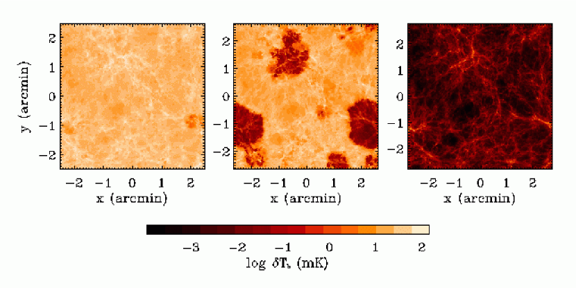
Once the Ly$\alpha$ and X-ray backgrounds become sufficiently strong, the 21 cm fluctuation pattern becomes independent of the temperature field. Even though the IGM will likely have a complex temperature field from continued shock heating, the brightness temperature is essentially unaffected: ${\mathcal{T}}\rightarrow 1$ in equation (1). The 21 cm signal therefore depends only on $\delta$ and ${x_{H}}$ during this phase. As a result, this epoch is more straightforward to consider from a theoretical standpoint than those described above. Several groups have analyzed it recently with both numerical [9, 18, 21] and analytic [53, 19, 20] techniques. In Figure 1, this approximation is accurate for all $z<20$ or so. An example of the evolving fluctuation pattern during this phase is shown in Figure 2.

The ultimate observational goal of the SKA is to map the evolving structure seen in the central panel of Figure 2. Structures in the IGM are causally related to the collapsed objects that are responsible for the photoionizing flux, and measuring these interelations will teach us about the first generations of stars and protogalaxies. However, direct imaging of the IGM in the 21cm line is a formidable challenge, and it is likely that the first steps in observing the 21cm signal from the EOR will be statistical studies that discriminate between evolutionary scenarios through measurements of (for example) the angular power spectrum.

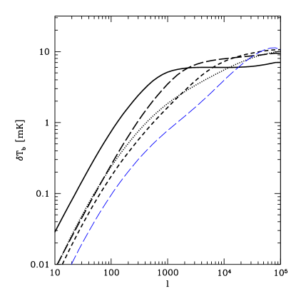
If uniform heating occurs sufficiently early compared to reionization, fluctuations in ${x_{H}}$ will also be negligible. In this case the 21 cm field traces the density and yields a direct measurement of the power spectrum of density fluctuations at $z\sim 10$ [48]. Such an observation would provide a sensitive probe of the growth of fluctuations during the early universe. The scales accessible to observations are linear at this time, so predictions of the fluctuation spectrum are relatively easy to make [48, 53]. Zaldarriaga et al. pointed out the mathematical analogy between measurements of CMB fluctuations and the 21 cm pattern, with the key difference that (because it is a line transition), 21 cm maps contain independent information at different frequencies. They showed how to describe the 21 cm fluctuations in terms of their angular power spectrum, which can in turn be computed from the three-dimensional power spectrum $P({\bf k})$. The fluctuations on a scale $l=2\pi/\theta$ are parameterized by the $C_{l}$ coefficients; the rms fluctuations are then given by $\langle\delta T^{2}\rangle^{1/2}=l(l+1)C_{l}/2\pi$ (note 1 arcmin corresponds to $l\approx 2\times 10^{4}$). In the case in which density fluctuations dominate, this is simply the usual linear power spectrum on the relevant scales. The fluctuations increase with decreasing angular scale, with a characteristic rms magnitude of several mK. The dotted curve in Figure 3 shows the angular power spectrum for this case of a universe with early, uniform heating at $z=18$ and with ${{\bar{x}}_{H}}=0.96$. This spectrum essentially registers the density fluctuations at $z=18$ and has no strong features.

Figure 3: An example of the time evolution of the 21 cm power spectrum. The time ordering is: dotted ($z=18$, ${{\bar{x}}_{H}}=0.96$), short-dashed ($z=15$, ${{\bar{x}}_{H}}=0.81$), long-dashed ($z=13$, ${{\bar{x}}_{H}}=0.52$) and solid ($z=12$, ${{\bar{x}}_{H}}=0.26$). The thick curves assume the reionization model of [19] while the thin dashed curve has each galaxy host an independent HII region ($z=13$, ${{\bar{x}}_{H}}=0.52$). The model assumes that each baryon inside a star forming galaxy produces $\zeta=40$ ionizing photons. From [19].

Once luminous sources become important, the primary source of fluctuations are the HII regions around ionizing sources, as shown in the middle panel of Figure 2. Predictions of the fluctuation pattern therefore depend on the particular model of reionization. One approach is to use numerical simulations to follow reionization. This is difficult for several reasons. First, radiative transfer remains a numerically challenging problem. It has usually only been added as a “post-processing” step to existing hydrodynamic simulations. Second, each simulation represents a substantial investment of computer time, and it is presently impractical to examine a large parameter space of reionization models. Third, locating typical ionizing sources (with $M\sim 10^{8}\mbox{ M${}_{\odot}$}$) at these redshifts requires high mass resolution, limiting the size of the computational box to $L<10h^{-1}$ comoving Mpc [44]. This severely limits the ability of numerical simulations to predict the 21 cm pattern on the arcminute scales (corresponding to several comoving Mpc) that would be accessible to the SKA. Nevertheless, much can be learned about the fluctuation pattern by examining simulations on small scales and extrapolating to larger scales [9, 18, 21]. These studies again suggest rms fluctuations $\delta T\sim 1$–$10\mbox{ mK}$ on scales of $\sim 1$–$10$ arcminutes ($l\sim 10^{3}$–$10^{4}$). The fluctuations also depend on the spectral bandwidth of the observation; they begin to be significantly suppressed when the radial scale (set by the spectral channel resolution) exceeds the transverse scale [53, 19]. Thus the relevant angular scales correspond to $\Delta\nu\sim 0.2$–$2\mbox{ MHz}$, or $\Delta z\sim 0.02$–$0.2$.

Analytic models present a different set of problems. Most importantly, reionization is a highly nonlinear process, and constructing an accurate model for the sizes and spatial distribution of HII regions is challenging. The simulations described above all show that the usual approximation – single HII regions surrounding each galaxy – does not describe overlap well. Instead, dense regions of the universe containing many galaxies rapidly grow into large ionized regions (with scales of a few comoving Mpc) once the ionizing flux escapes from the over-densities into the low density regions. Thus analytic treatments must take into account large scale features of the density field and not simply the regions near single galaxies. Moreover, there are a number of uncertain parameters (such as the clumpiness of gas in the IGM) that must be calibrated to simulations. Nevertheless, they offer the advantage of allowing efficient parameter studies and are not limited to small scales. Recently, [19] have developed an analytic model of reionization that includes the crucial features of the reionization process. The model relies on a simple extension of the Press-Schechter model [40] to compute the ionization pattern. It assumes that each galaxy can ionize a fixed multiple $\zeta$ of its own baryonic mass. It then determines the sizes of HII regions by finding those regions that contain enough collapsed gas (i.e., galaxies) to ionize the entire region; [19] showed that this can be approximated relatively simply through the “excursion set” formalism [4]. Given the background cosmology, the size distribution depends on only two parameters: the number of ionizations per collapsed baryon ($\zeta$), and the minimum halo mass that can host an ionizing source.

Given a model for reionization, we can then determine the observable characteristics of a 21 cm measurement. With high signal-to-noise maps, the size distribution of HII regions and the characteristics of reionization can be measured in a straightforward way. However, even without maps, statistical measurements are still extremely powerful. As described above, the simplest approach is to compute the power spectrum of 21 cm emission, which depends on both the size distribution of HII regions and fluctuations in the background density field. It is also relatively easy to interpret. Several examples of this simple statistic are shown in Figures 3 and 4 (both are taken from [19]). Figure 3 shows how the power spectrum evolves with time as the global neutral fraction decreases from unity to ${{\bar{x}}_{H}}=0.26$. As the HII regions appear and grow, they add a feature to the power spectrum on scales of several arcminutes ($l\sim 10^{3}$–$10^{4}$). The rms fluctuations increase by a factor of several on the characteristic scale of the HII regions, yielding a clear signature of reionization even in statistical measurements. The crucial point is that the power spectrum evolves rapidly through reionization, so its measurement will allow us to trace the time history of the HII regions. The thin curve shows an example where the sizes of HII regions are determined by individual galaxies (as if the galaxies were randomly distributed); it emphasizes the importance of the model of reionization in predicting the power spectrum features and, conversely, the power of 21 cm tomography to differentiate these models. Note that these Figures assume infinite frequency resolution; as discussed above, the fluctuations are significantly suppressed if the comoving radial distance exceeds the transverse distance [53, 19]. Until late in reionization (when the HII regions become very large), the desired bandwidths correspond to $\Delta z\sim 0.02$–$0.2$, and the redshift evolution within each bin is modest.

Figure 4: The 21 cm power spectrum in three different models of “double reionization.” The solid curves assume that the universe was uniformly ionized to ${{\bar{x}}_{H}}=0.5$ by a first generation of objects. The others assume that the first generation shut off while discrete bubbles still existed, again when ${{\bar{x}}_{H}}=0.5$. The second generation of sources completes reionization in all cases. In each model, the thin curves have a total ${{\bar{x}}_{H}}=0.46$ and the thick curves have ${{\bar{x}}_{H}}=0.27$. From [20].

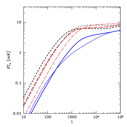
Figure 4 shows the kind of detailed information that we can extract from 21 cm tomography through the power spectrum [20]. Here we contrast predictions for two different prescriptions of “double reionization,” a scenario first considered in [6, 50]. Specifically, we consider the mechanism through which the first generation of highly ionizing sources shuts off. One possibility (solid curves) is that these sources ionize the universe more or less uniformly (or that they fully ionize the universe, which then recombines to a nearly uniform neutral fraction). Another possibility is that the first generation shuts off while its HII regions still exist, so that the neutral fraction is highly inhomogeneous during the transition. The two sets of dashed curves in Figure 4 show this prescription, with two different sets of properties for the first generation of sources. We see that, in the former case, the power spectrum and the bubble feature are significantly suppressed. In the latter scenario, however, the bubble feature is quite strong. Essentially, the first generation imprints a characteristic bubble size that persists until the second generation of sources are able to dominate the total number of ionizations. While these scenarios are no doubt overly simplified, they serve to illustrate the power of 21 cm observations.

It is important to note, however, that the power spectrum is only the simplest statistic available, essentially measuring the rms deviation as a function of angular scale. There are several other ways to approach the problem that take expicit advantage of the three-dimensional nature of the observations [37]. A related question is how to take advantage of the non-gaussian nature of the signal. Because fluctuations in the linear density field are gaussian, the power spectrum provides a complete characterization of that field. However, the ionized fraction is most assuredly not a gaussian random field; it is actually closer to a discrete variable (taking values zero or unity) in the simplest models. During the middle to late stages of reionization, other statistical properties may be better descriptors of the observations. For example, [20] argue that such statistics can help to distinguish the way in which reionization proceeds, whether from high-to-low density regions or from low-to-high density regions. More detailed methods to extract this information from the measurements are still required, however.

4 Observational Challenges & Instrument Requirements

4.1 Foreground Contamination

The surface brightness fluctuations $\delta T\sim 1$–$10\mbox{ mK}$ in the redshifted 21cm spectral line amount to ${\sim}10^{-5}$ of the brightness of the radio sky, which is dominated by the diffuse continuum synchrotron emission from the Milky Way Galaxy. The redshift range $6.2<z<20$ corresponds to $197>\nu>68\mbox{ MHz}$ [where $\nu=1420(1+z)^{-1}\mbox{ MHz}$]. In this frequency range, a good rule of thumb for the brightness temperature in the coldest directions is $T_{B}\approx 180(\nu/180{\rm MHz})^{-2.6}$K. The greatest complication imposed by the Galactic foreground is the increase in receiving system noise $T_{sys}$, since, according to the radiometer equation, the $rms$ noise in the antenna temperature $\Delta T\sim T_{sys}/\sqrt{\Delta\nu\;t_{int}}$ rises in proportion to sky brightness ($T_{sys}\geq T_{sky}$); achieving a low noise level must be accomplished by increasing integration time $t_{int}$, since the bandwidth $\Delta\nu$ is set by matching the expected widths of the spectral features (${\sim}0.2$ to 2 MHz). The brightness temperature of the radio sky increases toward the Galactic plane and is an order of magnitude higher toward the Galactic Center, necessitating the identification of selected high Galactic latitude regions in the sky for studying 21 cm emission from the EOR. The Galactic synchrotron halo is considered to be smooth on arcminute scales when mapped at normal sensitivities. However, the halo’s fluctuations at mK sensitivity remain to be explored.

To first order, conventional radio spectroscopic techniques for continuum subtraction should be capable of removing the foregrounds created by the Galactic synchrotron and by discrete extragalactic sources [5]. Interferometric antenna arrays are insensitive to smooth emission, and “resolve away” the DC term of the Fourier transform of the sky brightness. This leaves behind the structure caused by fluctuations in the Galactic foreground and the discrete radio source populations on the sky. Continuum source spectra are typically either power laws or vary only slowly from a power law. As a consequence, there are two steps to radio continuum subtraction, depending on the strength of the contaminating sources.

In the first step, the coordinates and spectrum of the strongest sources are measured, and the instrumental response to these sources is subtracted directly from the calibrated $u$-$v$ dataset. This leaves behind the many weaker sources, whose sum provides the continuum emission that populates the 1 to 20 arcminute resolution pixels in which we wish to measure the 21cm EOR emission.

Figure 5: Spectral line data cube. The spectral information for one R.A, Declination coordinate has been drawn in for emphasis. Since radio interferometers do not measure the ‘zero spacing flux density,’ the average flux density of each frequency plane of an observation cube is equal to zero. Spectral baseline removal involves fitting the residual continuum for each R.A-Dec pixel separately with a low-order polynomial. The fitted function is then subtracted from the values as a function of frequency. (from [5])

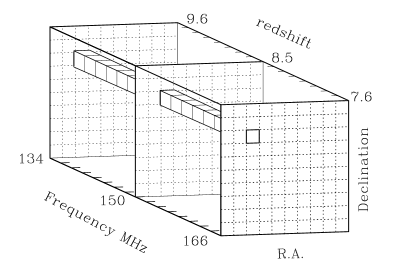
The second step operates on a pixel by pixel basis. The standard continuum subtraction operates on the intermediate stage data-product from spectral line observations, which is a data-cube (see Figure 5) composed of many image planes, with each plane of different frequency. The sums of the power law spectra with different spectral indices that fill a R.A.-Declination pixel may have spectral curvature, but these are adequately fit by second order polynomials. Several authors [11, 38, 10, 12] have raised concerns about the confusing effects of discrete source foregrounds, but conventional techniques are adequate for their removal, as illustrated in Figure 6.

Figure 6: An illustration of spectral baseline foreground subtraction for $3^{\prime}{\times}3^{\prime}$ pixels. Top panel: average integral flux density vs. frequency per pixel; this includes radio point sources but assumes that both the smooth Galactic contribution and the continuum sources brighter than $S_{cut}=100$ ${\mu}$Jy have been subtracted. Bottom panel: Open triangles are $rms$ deviations without continuum subtraction. Open squares are $rms$ residuals after linear spectral baseline subtraction. Filled circles are $rms$ residuals after quadratic baseline subtraction. In each case, the upper curve includes fluctuations from large scale structure , while the lower curve includes only Poisson statistical fluctuations (based on mean source count statistics). The horizontal dotted line marks the 10 mK level at 150 MHz, which is typical of the $rms$ fluctuations expected for the EoR signal. The righthand axis indicates $\log T_{B}$ for this pixel size (from [5]).

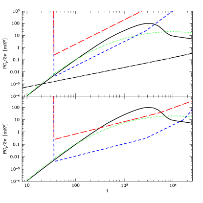
Other approaches to the problem of continuum removal have also been studied. They too rely on the spectral smoothness of the contaminants. One way to approach it is through the symmetries in the data cube in Fourier space [37]. Another is through frequency differencing [53], where neighboring planes in the data cube are subtracted from each other. This technique is similar to that described above except that the baseline subtraction is performed implicitly on the visibilities. The top panel of Figure 7 illustrates the level to which the foregrounds can be removed in the formalism of [53]. The solid and dotted curves show estimates of the 21 cm fluctuation spectrum at $z=10$, with and without HII regions. The dot-dashed curve shows the level to which the radio point source population predicted by [11] can be removed. It is clear that smooth foregrounds allow for more than the necessary precision in continuum removal.

Figure 7: Instrument sensitivities, as estimated by [53]. In both panels the dotted and solid curves show simple estimates for the 21 cm signal with and without reionization, respectively. The top panel shows the noise power spectrum (relevant for imaging) for LOFAR (long-dashed curve) and SKA (short-dashed curve). The bottom panel shows estimates for the errors in logarithmic $l$-bins of a statistical measurement of the power spectrum. The dot-dashed curve in the top panel shows the estimated level of residual foreground contamination from faint radio continuum sources.

Additional uncertainties surround the subtleties of instrumental response to the known (and yet to be discovered) foregrounds. For example, an array telescope actually senses every continuum source above the horizon at some level; the response has strong frequency dependence that increases with angular separation of each source from the telescope pointing coordinates. The distribution of sources (in strength and location) produces a pseudo-random superposition of these effects in the net response and could create spurious spectral features that will confuse 21cm line studies of the EOR. The solution may be to perform the data reduction for EOR surveys with access to all-sky radio source catalogues including coordinates, flux densities and spectral shapes. Another subtlety arises from the unknown polarization properties of the Galactic halo foreground, in which differential Faraday rotation of the synchrotron emission will enter in a frequency dependent way. If the telescope polarization response is not calibrated to high precision, then the rotating polarization vector could couple in the analysis to the measured intensity, and this could vary with frequency and position in the sky to mimic EOR signals. Much remains to be done in the exploration of instrumental effects, astrophysical foregrounds, and their interactions within the observational process.

4.2 SKA requirements

The goal of observing 21 cm emission from the EOR constrains the frequency coverage and array configuration of the telescope. For example, the SKA must be able to observe at frequencies on the order of $100\mbox{ MHz}$. The opacity in the Gunn-Peterson trough in high redshift quasars suggests that reionization may be ending at $z\sim 6$ [13]. If the universe is largely neutral (${{\bar{x}}_{H}}>0.3$) up to this epoch, even limiting the frequency coverage to $>150\mbox{ MHz}$ will provide valuable information about reionization. On the other hand, the CMB data presently indicates that reionization must begin at $z\sim 15$ [28]. If the universe is partially ionized beyond this point, the SKA would need to push to much lower frequencies in order to make 21 cm measurements. Unfortunately, precise constraints on the reionization history will probably not appear for several years (see §5) and may even be best determined by 21cm line observations. In any case, it appears that measurements of the formation of the first structures, as described in §3.1–3.2, could require frequency coverage below $70\mbox{ MHz}$.

Figure 8: Estimated detection limits of faint EOR features at four redshifts. The brightness fluctuation spectrum for a ${\Lambda}$CDM model assuming pure density fluctuations (following [18]) has been scaled upward by a factor of three to provide a rough measure of the 3-$\sigma$ peaks of brightness. We assume $\Delta\nu=0.5\mbox{ MHz}$ and neglect redshift space distortions. Solid lines indicate 5$\sigma$ detection limits for 100 and 1000 hour SKA observations, for different diameter arrays obtained by diluting 1 km² of collecting area to achieve higher angular resolution. Dotted curves do the same for a LOFAR array.

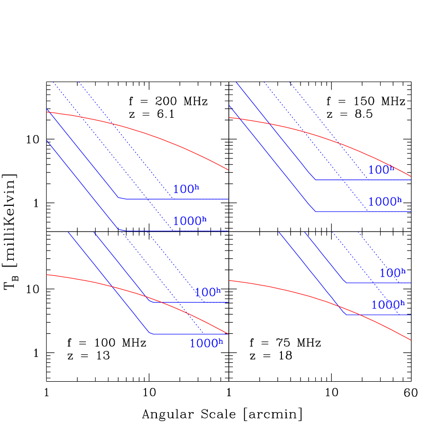
Sensitivity to faint fluctuations in surface brightness against the bright radio sky at these frequencies will require a large collecting area. The achievable uncertainty in surface brightness ${\Delta}T_{b}\approx\Delta T_{a}/\eta_{f}=T_{sys}/\eta_{f}\sqrt{\Delta\nu\;t_{int}}$ for emission that fills the array beam depends on the array filling factor $\eta_{f}$. Because the fluctuation spectrum falls off toward large angular scales, the array must have diameter of $\sim$3000 wavelengths if the beam is to match $1^{\prime}$ structure. On the other hand, to obtain surface brightness sensitivity, the aperture cannot be too severely diluted due to the $\eta_{f}$ dependence.

The filling factor requirement, along with the frequency dependence of the radio sky, are illustrated in Figure 8. This Figure provides an overview of the issues that influence the ability of the SKA to map specific features in the EOR, which will be crucial for relating structures in the IGM to star forming regions observed at infrared and possibly millimeter wavelengths. The Figure has four panels in order to show the increasing degree of difficulty of the observation toward higher redshifts: as the frequency decreases, the sky brightness and the diffraction limited resolution worsen. The signal predictions assume pure density fluctuations (i.e., they neglect the contribution from HII regions) and that $T_{S}>>T_{CMB}$ everywhere. They are generated as described in [18] (who in turn followed [48]), assuming $\Delta\nu=0.5\mbox{ MHz}$ and neglecting redshift space distortions (which will amplify the signal by a small factor). Note that we show $3\sigma$ peaks in order to illustrate the brightest features. The instrumental sensitivity is best for the largest angular scales ($>10^{\prime}$) since the array beam would be filled by the brightness fluctuations for a filled array ($\eta_{f}=1$). For finer angular scales, the aperture must be diluted in order to match the beam to the fluctuations, causing the sensitivity to deteriorate. For this figure, the noise level is set by the $T_{sys}\approx T_{sky}$, with the assumption that residuals from foreground subtraction make a negligible contribution.

The statistical measures of the fluctuation power spectrum have somewhat different dependencies. The short-dashed curve in the upper panel of Figure 7 shows the approximate noise power spectrum for the SKA assuming one month of continuous observing, a $0.4\mbox{ MHz}$ channel, and $A_{\rm eff}/T_{\rm sys}=2\times 10^{5}{\rm m}^{2}/\mbox{ K}$ (see reference [53] for details). This curve essentially shows the noise per visibility as a function of scale and is analogous to the noise per pixel in a real-space map. The long-dashed curve shows the approximate noise for the Low Frequency Array (LOFAR). We can see clearly that (because the sky brightness is essentially fixed) high signal-to-noise maps require collecting areas on the order of a square kilometer; even then they will be difficult. We note that this sensitivity curve was constructed with several fairly crude approximations and is only accurate to a factor of a few. It depends in detail on the configuration of the array, the antenna beams, the correlator properties, and the observing strategy. In the future, these questions must be addressed in more detail. Also note that, on the scales of the HII regions, the contrast between ionized and neutral regions will be substantially larger than the simple rms variation shown here; in this sense map-making during the middle stages of reionization will be easier than suggested by this plot.

Of course, statistical properties are much easier to measure than maps, because we can average over many measurements on each scale. The requirements for the signal-to-noise ratio on each angular scale are therefore much weaker. The bottom panel of Figure 7 shows the estimated errors in such a measurement for the SKA and LOFAR, assuming logarithmic bins in $l$-space and a $100$ square degree field of view. We see that the power spectrum of the fluctuations can be measured with good accuracy even with collecting areas smaller than a square kilometer provided that the field of view is large.

Finally, the most important angular scales for measuring the fluctuations are in the range $\sim 1$–$20^{\prime}$, which contain both the peak of fluctuations in the linear density field and the expected scale of HII regions during most of reionization (at least in the model of [19]). This suggests that the SKA have a compact core with baselines $\sim 3\mbox{ km}$ that contains a substantial fraction of the collecting area (Figure 7 assumes that $20\%$ of the antennae are inside a core of diameter $3\mbox{ km}$). While long baselines will be useful for point source removal, 21 cm tomography requires heavy emphasis on the compact core.

5 Conclusions

Understanding reionization is one of the major goals of cosmology. We have argued that 21 cm tomography is a particularly powerful way to attack the problem, but there are several others. We are already reaching the limits of observations with the Ly$\alpha$ forest; observations of complete Gunn-Peterson troughs at $z\sim 6$ indicate that this tool cannot be taken to substantially higher redshifts. Moreover, Ly$\alpha$ absorption is so strong that even measurements of zero transmission do not imply a fully neutral medium. Thus, more detailed constraints from optical observations must rely on modeling of the HII region around quasars [51, 35], measurements of the detailed shape of the Ly$\alpha$ absorption profile [36] in (for example) gamma-ray burst afterglow spectra, or the careful interpretation of Ly$\alpha$ emission lines from high-redshift galaxies [39, 32, 41, 22, 7]. While invaluable, these methods are fraught with uncertainty.

More detailed measurements of the CMB will also yield more information about the ionization history. Most importantly, WMAP and Planck will better measure the total optical depth to electron scattering and place a strong integral constraint on the ionization history. However, the CMB power spectrum is relatively insensitive to the evolution of the ionized fraction [25], and strong constraints will probably have to await space-borne missions beyond Planck. (Note that the reionization signal appears on larger angular scales than ground-based or balloon experiments can easily probe.)

Finally, direct observations of high-redshift protogalaxies, with (for example) the James Webb Space Telescope or the upcoming generation of twenty-meter ground-based telescopes, will obviously teach us an enormous amount about the growth of the first luminous objects. However, we will still have only indirect measurements of the IGM structure and the process of reionization.

Thus it seems that 21 cm tomography provides a unique and invaluable probe of the high-redshift universe. No other technique can measure the three-dimensional distribution and time evolution of neutral gas in such detail. Also, only 21 cm measurements can extend into the era before the formation of the first luminous objects (see §3.1 and 3.2) to map the initial stages of structure formation. Provided that the technical challenges described in §4 can be overcome, there is no doubt that 21 cm tomography will revolutionize our understanding of reionization and the early universe. While statistical measurements of the distribution of ionized gas may be possible with LOFAR or some other instrument before SKA, we expect that a collecting area near one square kilometer will be required in order to make high signal-to-noise maps of the neutral gas distribution.

On the other hand, we expect that these measurements will complement the next generation of infrared, X-ray, and CMB instruments. For example, comparing the distribution of ionized gas to the luminous sources in a cosmological volume would show explicitly how those sources are responsible for ionization. We can also use 21 cm observations of large ionized regions to locate bright quasars and in principle to constrain many of their unknown properties, including their ages [52] and spectra [48].

Finally, we note that reionization is an evolving field. The data are continuing to improve, and our theoretical understanding is advancing even more rapidly. At the same time, the amount of attention focused on 21 cm studies has expanded dramatically, and our understanding of the instrumental and data analysis challenges is improving by leaps and bounds. This review has presented a snapshot of the field in May 2005. Our expectations will no doubt change in many ways (some unexpected) before the SKA begins observations.

References

- [1] A. C. Allison & A. Dalgarno, ApJ 158 (1969) 423
- [2] R. Barkana & A. Loeb, Physics Reports 349 (2001) 125
- [3] R. H. Becker et al., AJ 122 (2001) 2850
- [4] J. R. Bond, S. Cole, G. Efstathiou & N. Kaiser, ApJ 379 (1991) 440
- [5] A.G. de Bruyn, F.H. Briggs, & M. van Haarlem (2004), in prep
- [6] R. Cen, ApJL 591 (2003) L5
- [7] R. Cen, Z. Haiman, & A. Mesinger, ApJL submitted (astro-ph/0403419)
- [8] X. Chen & J. Miralda-Escudé, ApJ 602 (2004) 1
- [9] B. Ciardi & P. Madau, ApJ 596 (2003) 1
- [10] A. Cooray & S. R. Furlanetto, ApJL 606 (2004) L5
- [11] T. Di Matteo, R. Perna, T. Abel, M. J. Rees, ApJ 564 (2002) 576
- [12] T. Di Matteo, B. Ciardi, & F. Miniati, MNRAS submitted (astro-ph/0402322)
- [13] X. Fan et al., AJ 123 (2002) 1247
- [14] G. B. Field, Proc. IRE 46 (1958) 240
- [15] G. B. Field, ApJ 129 (1959) 525
- [16] G. B. Field, ApJ 129 (1959) 551
- [17] S. R. Furlanetto & A. Loeb, ApJ 611 (2004) 642
- [18] S. R. Furlanetto, A. Sokasian, & L. Hernquist, MNRAS 347 (2004) 187
- [19] S. R. Furlanetto, M. Zaldarriaga, & L. Hernquist, ApJ in press (astro-ph/0403697)
- [20] S. R. Furlanetto, M. Zaldarriaga, & L. Hernquist, ApJ in press (astro-ph/0404112)
- [21] N. Y. Gnedin, & P. A. Shaver, ApJ 608 (2004) 611
- [22] N. Y. Gnedin & F. Prada, ApJ 608 (2004) L77
- [23] J. E. Gunn & B. A. Peterson, ApJ 142 (1965) 1633
- [24] Z. Haiman & G. P. Holder, ApJ 595 (2003) 1
- [25] G. P. Holder, Z. Haiman, M. Kaplinghat, & L. Knox, ApJ 595 (2003) 13 13
- [26] L. Hui & Z. Haiman, ApJ 596 (2003) 9
- [27] I. T. Iliev, P. R. Shapiro, A. Ferrara, & H. Martel, ApJL 572 (2002) L123
- [28] A. Kogut et al., ApJS 148 (2003) 161
- [29] A. Kogut et al., ApJ, submitted (astro-ph/0402578)
- [30] A. Kumar, T. Padmanabhan, & K. Subramanian, MNRAS 272 (1995) 544
- [31] A. Loeb & M. Zaldarriaga, PRL 92 (2004) 211301
- [32] A. Loeb, R. Barkana, & L. Hernquist, ApJ submitted (astro-ph/0403193)
- [33] P. Madau, A. Meiksin, & M. J. Rees, ApJ 475 (1997) 429
- [34] A. Meiksin, in Perspectives on Radio Astronomy: Science with Large Antenna Arrays, M. P. van Haarlem ed. (1999) 37
- [35] A. Mesinger, Z. Haiman, & R. Cen, ApJ submitted (astro-ph/0401130)
- [36] J. Miralda-Escudé, ApJ 501 (1998) 15
- [37] M. Morales & J. Hewitt, ApJ in press (astro-ph/0312437)
- [38] S. P. Oh & K. J. Mack, MNRAS 346 (2003) 871
- [39] R. Pello et al., A&A 416 (2004) L35
- [40] W. H. Press & P. Schechter, ApJ 187 (1974) 425
- [41] M. Ricotti et al., MNRAS 352 (2004) L21
- [42] D. Scott & M. J. Rees, MNRAS 247 (1990) 510
- [43] P. A. Shaver, R. A. Windhorst, P. Madau, & A. G. de Bruyn A&A 345 (1999) 380
- [44] A. Sokasian, T. Abel, L. Hernquist, & V. Springel, MNRAS 344 (2003) 607
- [45] A. Songaila, AJ 127 (2004) 2598
- [46] D. N. Spergel et al., ApJS 148 (2003) 175
- [47] T. Theuns et al., ApJL 567 (2002) L103
- [48] P. Tozzi, P. Madau, A. Meiksin, & M. J. Rees, ApJ 528 (2000) 597
- [49] S. A. Wouthuysen, AJ 57 (1952) 31
- [50] J. S. B. Wyithe & A. Loeb, ApJL 588 (2003) L69
- [51] J. S. B. Wyithe & A. Loeb, Nature 427 815
- [52] J. S. B. Wyithe & A. Loeb, ApJ 610 (2004) 117
- [53] M. Zaldarriaga, S. R. Furlanetto, & L. Hernquist, ApJ 608 (2004) 622