Probing the Eclipse of J0737$-$3039A with Scintillation

Abstract

We have examined the interstellar scintillations of the pulsars in the double pulsar binary system. Near the time of the eclipse of pulsar A by the magnetosphere of B, the scintillations from both pulsars should be highly correlated because the radiation is passing through the same interstellar plasma. We report confirmation of this effect using 820 and 1400 MHz observations made with the Green Bank Telescope. The correlation allows us to constrain the projected relative position of the two pulsars at closest approach to be $4000\pm 2000$ km, corresponding to an inclination that is only $0.29\pm 0.14^{\circ}$ away from 90^∘. It also produces a two-dimensional map of the spatial correlation of the interstellar scintillation. This shows that the interstellar medium in the direction of the pulsars is significantly anisotropic. When this anisotropy is included in the orbital fitting, the transverse velocity of the center of mass is reduced from the previously published value of 141 $\pm 8.5$ km s^-1 to 66 $\pm 15$ km s^-1.

1. Introduction

The two pulsars in the recently discovered double pulsar binary system, “A” and “B”, have periods of 23 ms and 2.8 s, respectively. They are in a highly relativistic orbit with period of only 2.4 hrs and eccentricity of 0.088 and have an average separation of only 2.9 lt-s Burgay et al. (2003); Lyne et al. (2004). The phenomenology exhibited by this system is extremely rich. Pulsar A is eclipsed when it passes behind pulsar B Lyne et al. (2004); Kaspi et al. (2004). Modulation of the eclipse with the period of B is consistent with the eclipse being caused by synchrotron absorption by the plasma surrounding the magnetosphere of B McLaughlin et al. 2004b . Throughout the orbit, the flux density of the B pulsar varies dramatically and systematically, indicating significant interaction between the two pulsars Ramachandran et al. (2004); McLaughlin et al. 2004a . Only $\sim$ 0.5 kpc away, and with orbital velocities reaching over 300 km s^-1, this system is an ideal laboratory for studies of general relativity, binary kinematics and, in the case of this paper, the binary orbital geometry and the interstellar medium.

Pulse timing measurements provide many of the parameters of the system, including the exact masses of the two pulsars, with exquisite precision. From measurements of the Shapiro delay, the inclination of the system can be constrained to be 87${}^{\circ}\pm 3^{\circ}$ Lyne et al. (2004). Measurements of the time scale of the interstellar scintillation (ISS) over an orbit can be used to estimate the orbital inclination, the longitude of periastron, and the transverse velocity of the center of mass of the system. This technique was first suggested by Lyne & Smith (1982) and has been applied to PSR B0655+64 Lyne (1984) and PSR J1141$-$6545 (Ord, Bailes & van Straten 2002). In general, there are two solutions for the orbital inclination that fit the data equally well, but one may fit the expected mass of the pulsar better. In the case of the double pulsar system, the masses of A and B are already accurately determined through timing, removing this ambiguity.

Ransom et al. (2004) (hereafter R04) applied the technique to the double pulsar system, calculating an inclination of $88.7^{\circ}\pm 0.9^{\circ}$ and transverse velocities of the center of mass parallel and perpendicular to the orbital line of nodes in the plane of the sky of $V_{\rm par}=96.0\pm 3.7$ km s^-1 and $V_{\rm perp}=103.1\pm 7.7$ km s^-1, respectively. This calculation relied on the implicit assumption that the turbulence in the interstellar medium (ISM) is isotropic. If the turbulence is anisotropic the transverse velocity estimated by this method depends strongly on the axial ratio and orientation of the anisotropy and can be much lower than for isotropic turbulence. Note that neither this method nor timing can resolve the sense of the inclination, i.e. whether the angular momentum vector points towards or away from the Earth. Furthermore neither method can resolve the direction of the parallel velocity with respect to the angular momentum vector.

In this paper, we examine the correlations of the A and B pulsars’ scintillations near the time of the A eclipse, i.e. when the lines of sight are closest to one another. We show how these correlations constrain the orbital geometry more tightly than was previously possible and partially resolve the ambiguity in the sense of the inclination and the direction of the perpendicular velocity. We also show that the ISM is significantly anisotropic and that the transverse velocity of the center of mass is much smaller than was estimated with an isotropic model of the ISM.

2. Observations and Analysis

Observations of the double pulsar system with the 100-m Green Bank Telescope took place in December 2003 and January 2004 under an “Exploratory Time” proposal as reported by R04. The 820-MHz data used for this analysis were acquired with the GBT Spectrometer SPIGOT card with a sampling time of 40.96 $\mu$s on each of 1024 frequency channels covering a 50-MHz bandwidth. The 1400-MHz data were acquired using the Berkeley-Caltech Pulsar Machine (BCPM) using a sampling interval of 72 $\mu$s on each of 96 channels covering a 96-MHz bandwidth. A total of 5 hours of data at 820 MHz and 6.1 hours of data at 1400 MHz were obtained.

Our first step in the analysis of these data was to create dynamic spectra for each pulsar in each frequency band. In order to do this, we folded each frequency channel modulo the pulsar period using the ephemeris from Lyne et al. (2004) and freely available software tools (Lorimer et al. 2000). Individual frequency channels were shifted with respect to each other using a dispersion measure (DM) of 48.9 cm^-3 pc (Lyne et al. 2004). Individual profiles were added so that the time resolution was 10 s at 1400 MHz and 5 s at 820 MHz. We formed on-pulse spectra by integrating over an “on-pulse” window and subtracted off-pulse spectra formed by integrating over an equivalent “off-pulse” window. We did not attempt to correct for variations in the system gain over the bandpass because such corrections increased the noise and the gain variations did not appear to bias the results. The dynamic spectra are essentially the same as those shown by R04.

In order to estimate the time scale we first split the dynamic spectrum of A into segments of length 5.3 min and 10 min at 820 and 1400 MHz respectively, subtracted the mean from each spectrum, and then computed the temporal autocorrelation function $\rho(t)$ of each segment. We then fit a theoretical model beginning at the second point to determine the time scale $\Delta t_{d}$, as defined in Cordes (1986). We used the theoretical form for a Kolmogorov scattering medium $\rho(t)=\exp[-(t/\Delta t_{d})^{5/3}]$ rather than the commonly used Gaussian function $\rho(t)=\exp[-(t/\Delta t_{d})^{2}]$. The rms error in the $\Delta t_{d}$ estimates is much smaller at 820 MHz because the 820 MHz spectra have 10 times as many degrees of freedom as the 1400 MHz spectra.

Normally, scintillation is thought of as primarily a temporal process $I(t)$, i.e. “twinkling” caused by the motion of a spatial diffraction pattern $I({\bf r})$ past the observer with transverse velocity ${\bf V_{\rm ISS}}$. If the diffraction pattern is isotropic with spatial scale $S_{\rm ISS}$, the time series will have a time scale $T_{\rm ISS}=S_{\rm ISS}/|{\bf V_{\rm ISS}}|$. The spatial scale can be estimated from the bandwidth and the distribution of turbulence along the line of sight Cordes & Rickett (1998), so that one may estimate the velocity as $|{\bf V_{\rm ISS}}|=S_{\rm ISS}/T_{\rm ISS}$. The transverse velocity of the center of mass ($V_{\rm par},V_{\rm perp}$) and $S_{\rm ISS}$ are derived by fitting a model to the measured $|{\bf V_{\rm ISS}}(\phi)|$, where $\phi$ is the orbital phase. As noted by R04 the result is calibrated relative to the precisely known orbital velocity of the A pulsar. However, if the ISM is anisotropic, $S_{\rm ISS}$ depends on the direction of ${\bf V_{\rm ISS}}$ and the model must be modified accordingly (see §4). Our estimate of ($V_{\rm par},V_{\rm perp}$) using an isotropic model matches that of R04 within their quoted errors.

3. Cross-correlation of Pulsars A and B

Near the time of the eclipse of pulsar A, the lines of sight to the two pulsars will pass through nearly the same ISM and their scintillations should therefore be correlated. The pulsars sample the ISM at their projected locations ${\bf r_{A}}(t_{A})={\bf r_{A}}(0)+{\bf V_{A}}t_{A}$ and ${\bf r_{B}}(t_{B})={\bf r_{B}}(0)+{\bf V_{B}}t_{B}$ which, of course, depend on the times of observations. ${\bf V_{A}}$ and ${\bf V_{B}}$ are the vector sums of the transverse center of mass velocity ($V_{\rm par},V_{\rm perp}$) with the transverse orbital velocities $V_{AO}$ and $V_{BO}$. We can regard ${\bf V_{A}}$ and ${\bf V_{B}}$ as essentially constant near the time of the eclipse. We define $t_{A}$ and $t_{B}$ with respect to the time of the superior conjunction of A (where A is at least partially eclipsed). Likewise, ${\bf r_{A}}$ and ${\bf r_{B}}$ are defined with respect to the position of A at $t_{A}=0$. We define our coordinates as parallel and perpendicular to the line of nodes. Since the inclination is so close to 90 degrees, this is essentially parallel to pulsar B’s orbital velocity. The location of B at superior conjunction is ${\rm y_{B}(0)}$. The spatial cross correlation $\rho({\bf s}={\bf r_{A}}-{\bf r_{B}})$ cannot be computed as a time average because the baseline ${\bf s}$ varies rapidly with time. However the averaging can be done over frequency because ISS also modulates the spectrum, and the spectral modulation is independent of velocity.

In Figure 1, we present the cross-correlation $\rho(t_{A},t_{B})$ of the dynamic spectra of A and B at 1400 MHz. This is an average of all three eclipses in the data set. The spectra were smoothed over three samples (30 s) in time, retaining 10 s sampling, in order to optimize the signal to noise ratio. The correlation is normalized by the square root of the product of the total variance from A and B, i.e. including noise. The marginal distributions show the fluxes of A and B as a function of time. The intensity of B is very low more than 200 s before the eclipse, making it impossible to correct the normalization for system noise over the range of ($t_{A},t_{B}$) plotted in Figure 1. We corrected the correlation for noise in the region where the flux of B is significant ($t_{B}>-200$ s) and fitted an elliptical Kolmogorov model to the data. The peak correlation was 81% at $t_{AP}=33.4\pm 2.8$ sec (i.e. after the eclipse) and $t_{BP}=-22.7\pm 1.2$ sec (i.e. before the eclipse). The noise correction is uncertain because the noise is not stationary and we believe that the peak correlation is consistent with 100%. At this peak the A and B trajectories ${\bf r_{A}}(t_{A})$ and ${\bf r_{B}}(t_{B})$ intersect as shown in Figure 2.

\psfrag{Ta(s)}{$\it t_{A}$ (s)}\psfrag{Tb(s)}{$\it t_{B}$ (s)}\includegraphics[scale={0.50}]{f1.eps}

Figure 1.— The cross correlation $\rho(t_{A},t_{B})$ averaged over the three eclipses measured. The flux densities of A and B are shown as marginal distributions, showing clearly the eclipse of A and the strong orbital variation of B. The correlation has not been corrected for system noise.

The intersection equation ${\bf r_{A}}(t_{AP})={\bf r_{B}}(t_{BP})$ yields ${\bf V_{A}}t_{AP}={\bf V_{B}}t_{BP}+{\rm y_{B}(0)}$. The x component provides a solution for the center of mass velocity component $V_{\rm par}=(V_{AO}t_{AP}+V_{BO}t_{BP})/(t_{AP}-t_{BP})$. Using the known orbital speeds at the time of the eclipse ($V_{AO}=329$, $V_{BO}=352$ km s^-1 ), we directly obtain $V_{\rm par}=53\pm 17$ km s^-1 . This is clearly inconsistent with $V_{\rm par}=96\pm 4$ km s^-1 obtained by R04. We will show later that this inconsistency is due to anisotropic scattering in the interstellar plasma. The y component of the intersection equation yields $V_{\rm perp}={\rm y_{B}(0)}/(t_{AP}-t_{BP})$. As $(t_{\rm AP}-t_{\rm BP})$ is positive, we know that $V_{\rm perp}$ is in the same direction as ${\rm y_{B}(0)}$, but we cannot determine if they are parallel or anti-parallel to the angular momentum. Using the value $V_{\rm perp}=103\pm 7.7$ km s^-1 determined by R04 we find ${\rm y_{B}(0)}=5780$ km. The trajectories ${\bf r_{A}}(t_{A})$ and ${\bf r_{B}}(t_{B})$ shown in Figure 2 are calculated using the velocities determined by R04 assuming isotropic scattering and this value of ${\rm y_{B}(0)}$. The alternative track for ${\bf r_{B}}(t_{B})$ shown without a dotted line corresponds to the ambiguity in the sense of the orbital inclination. The inclination is 0.41^∘ from 90^∘ if ${\rm y_{B}(0)}$ is correct. However anisotropic scattering also modifies $V_{\rm perp}$ as we will show later, and this reduces ${\rm y_{B}(0)}$. While the pulsars will again sample similar paths through the ISM when B passes behind A, the emission from B is very weak at this crossing and we cannot repeat this analysis for that part of the orbit.

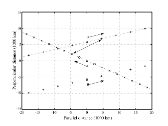
Figure 2.— The trajectories of the A and B pulsars referenced to the location of the A pulsar at the time of its eclipse. The sample spacing is 10 s. The duration of the eclipse is indicated by open circles on the A trajectory, otherwise denoted by crosses connected by a dotted line. The plus signs connected by a dotted line represent the B trajectory for an inclination of 90.41^∘, corresponding to an ${\rm y_{B}(0)}$ of 5780 km. The plus signs with no dotted line show the B trajectory for the opposite sense of inclination. To illustrate the mapping more clearly, the baseline ${\bf s}={\bf r}_{A}(20)-{\bf r}_{B}(10)$ where $(t_{A},t_{B})=(20,10)$ is indicated by the double-ended arrow.

The temporal correlation in Figure 1 can be mapped into a spatial correlation $\rho({\bf s}={\bf r_{A}}(t_{A})-{\bf r_{B}}(t_{B}))$ if the velocities are known. This will allow us to examine the isotropy assumption directly. The spatial correlation resulting from the trajectories shown in Figure 2 is displayed in Figure 3. Here we have displayed a more limited range than in Figure 1 and we have corrected the normalization of the correlations for system noise over the entire plot. This reduces the bias due to system noise but it creates a diagonal stripe of spurious correlation running from (0, $-30000$ km) to (60000 km, 0) where the flux of pulsar B is very low (so the correction factor is very large). When ${\rm y_{B}(0)}$ is chosen correctly, the (noise-corrected) spatial correlation should be symmetrical around the origin. The value of ${\rm y_{B}(0)}$ which best centers the correlation is 4000 km. Note that because the spatial scale of the ISS is larger than that of the eclipse, the spatial correlation is not badly distorted by A’s eclipse. This apparent correlation is clearly anisotropic with an axial ratio near 2. However, since the mapping used the center of mass velocity obtained from an isotropic scattering model, this result is not self-consistent. Consequently, in §4 we repeat the orbital time scale fitting including anisotropy.

\psfrag{Xa - Xb $km$}[c]{${\rm x_{A}-x_{B}}$ ($10^{4}$ km)}\psfrag{Ya - Yb $km$}[c]{${\rm y_{A}-y_{B}}$ ($10^{4}$ km)}\includegraphics[scale={0.50}]{f3.eps}

Figure 3.— The apparent spatial correlation $\rho(s_{x},s_{y})$ at 1400 MHz, where $({\rm x_{A},y_{A}})$ and $({\rm x_{B},y_{B}})$ are the parallel and perpendicular components of ${\bf r}_{A}$ and ${\bf r}_{B}$, respectively. The mapping velocities are those determined from an isotropic scattering model. An ellipse with an axial ratio of 2 with the major axis at –50^∘ is drawn over the correlation to guide the eye. Here ${\rm y_{B}(0)}=4000$ km is used because it provides a more symmetric result than the 5780 km shown in Figure 2.

In Figure 4, we present the temporal correlation at 820 MHz, averaged over three eclipses. As at 1400 MHz, the spectra were smoothed over three sample intervals but the original 5 s sampling was retained. The spatial scale of ISS scales as $\lambda^{-2/\alpha}$ (eqn 44 of Rickett, 1977), where $\alpha=5/3$ for a Kolmogorov scattering medium. Thus the scale at 820 MHz is smaller than at 1400 MHz by a factor of $(820/1400)^{1.2}=0.53$, making it more comparable with the size of the eclipse. The raw correlations are lower than at 1400 MHz, but the estimation error is also lower. When the normalization is corrected for system noise the peak correlation reaches 100%. The spatial correlation at 820 MHz is shown in Figure 5, using the same ($V_{\rm par},V_{\rm perp}$) as for Figure  3. The correlation is also anisotropic, but the axial ratio is somewhat smaller than at 1400 MHz. We attribute the differences to the greater distortion by the eclipse at 820 MHz. To make this correlation symmetric about the origin we reduced ${\rm y_{B}(0)}$ to 3000 km. It is possible that the difference between this value of ${\rm y_{B}(0)}$ and that of 4000 km at 1400 MHz is due to differential refraction in the magnetosphere of B, but the difference is comparable with our estimate of the error. Allowing for this possibility we estimate that ${\rm y_{B}(0)}=4000\pm 2000$ km which corresponds to an inclination of $0.29^{\circ}\pm 0.14^{\circ}$ away from 90^∘.

\psfrag{Tb $s$}{$\it t_{B}$ (s)}\psfrag{Ta $s$}{$\it t_{A}$ (s)}\includegraphics[scale={0.45}]{f4.eps}

Figure 4.— The average correlation $\rho(t_{A},t_{B})$ for the three eclipses at 820 MHz. The sample interval is 5 s. The origin is offset because the first eclipse was very close to the start of the observation. The spatial scale of the ISS is much smaller than at 1400 MHz and is comparable to the scale of the eclipse, so that the correlation is heavily distored by the eclipse, and perhaps by propagation through the B magnetosphere. However, the peak remains in the lower left, as at 1400 MHz (Figure 1).

\psfrag{Xa - Xb $km$}[c]{${\rm x_{A}-x_{B}}$ ($10^{4}$ km)}\psfrag{Ya - Yb $km$}[c]{${\rm y_{A}-y_{B}}$ ($10^{4}$ km)}\includegraphics[scale={0.50}]{f5.eps}

Figure 5.— The spatial correlation $\rho(s_{x},s_{y})$ at 820 MHz. The edge of the transformation window can be seen because the first eclipse was very close to the start of the observations. This correlation has been corrected for 95% of the system noise. Full correction produced high errors during the eclipse. The ellipse drawn over the 1400 MHz data has been scaled down by a factor of 53% and over-plotted here.

4. Anisotropy Analysis for J0737$-$3039

While the previous analysis showed that the ISS is anisotropic, the spatial mapping was carried out with velocities determined using an isotropic scattering model, hence the result is not self-consistent. In this section, we therefore modify the orbital fitting to include anisotropy and find a self-consistent spatial mapping.

If the spatial correlation has elliptical symmetry, it can be written as $\rho({\bf s})=f(Q({\bf s}))$, where $Q({\bf{s}})=as_{x}^{2}+bs_{y}^{2}+cs_{x}s_{y}$ is the quadratic form which describes the ellipse. The form of $f$ is less important; for example, for a Kolmogorov power law, $\rho({\bf s})={\rm exp}[-(Q({\bf s})/S_{\rm ISS}^{2})^{5/6}]$. Here, $S_{\rm ISS}$ is the 1/$e$ spatial scale. The temporal correlation $\rho(t)$ is determined by substitution of ${\bf s}={\bf V}t$, giving $\rho(t)=f(Q({\bf V})t^{2})$, where ${\bf V}$ is the transverse velocity of the pulsar. The width $T_{\rm ISS}$ of the temporal correlation is given by $Q({\bf V})T_{\rm ISS}^{2}=S_{\rm ISS}^{2}$. In previous work, $S_{\rm ISS}$ has been calculated from a theoretical scattering model, with the theoretical velocity ${\bf{\bf V_{A}}}(\phi)$ fit to the measured $|{\bf V_{\rm ISS}}(\phi)|=S_{\rm ISS}/T_{\rm ISS}(\phi)$ with an arbitrary scale factor (e.g. Ord et al. 2002). However, the preliminary calculation of $S_{\rm ISS}$ is not necessary, so we have simply included $S_{\rm ISS}$ in the fit instead of using a scale factor. The model we fit to the measured values of $(1/T_{\rm ISS})$ for pulsar A is $[Q({\bf{\bf V_{A}}})]^{0.5}/S_{\rm ISS}$, and the fitting parameters are $V_{\rm par}$, $V_{\rm perp}$, and $S_{\rm ISS}$. The input parameters $A_{r}$ and $\theta$, where $A_{r}$ is the axial ratio of the fitted ellipse and $\theta$ is the position angle of the ellipse, must be given. The coefficients of the quadratic form are: $a={\rm cos}^{2}\theta/A_{r}+A_{r}{\rm sin}^{2}\theta$; $b={\rm sin}^{2}\theta/A_{r}+A_{r}{\rm cos}^{2}\theta$; and $c=2{\rm sin}\theta{\rm cos}\theta(1/A_{r}-A_{r})$. With this definition, $S_{\rm ISS}$ is the geometric mean of the major and minor axis scales.

To find a self-consistent solution we use the 1400 MHz correlations, which are least distorted by the eclipse, with the 820 MHz measurements of $T_{\rm ISS}(\phi)$ which have the higher signal to noise ratio. We then assumed an axial ratio and orientation; computed the resulting center of mass velocity by fitting to the time scale vs orbital phase; used that velocity to create a spatial correlation; and estimated the axial ratio and orientation of that spatial correlation. When the correct axial ratio has been assumed it will be the same as that of the spatial correlation. We did this for a grid of axial ratio and orientation up to axial ratios of 10. To define a goodness of fit we used the technique suggested by Grall et al. (1997). We plotted the assumed anisotropy and that of the resulting spatial correlation on a modified Poincaré sphere and used the distance between them as a measure of the error. The best solution, near $A_{r}=4$ and $\theta=-15^{\circ}$ with ${\rm y_{B}(0)}=4000$ km, is shown in Figure 6. We find acceptable solutions for $A_{r}\geq 3$ with $-20^{\circ}\leq\theta\leq-10^{\circ}$. We searched $A_{r}$ as large as 10, but we find it hard to believe that such axial ratios are feasible without corroborating evidence. The center of mass velocity is minimum at $A_{r}=4$. If we restrict the axial ratio to $3\leq A_{r}\leq 6$ then $51\leq|(V_{\rm par},V_{\rm perp})|\leq 81$ km s^-1. The estimated $V_{\rm par}=53\pm 17$ km s^-1 obtained earlier is consistent with this result and it may be possible with more data to use $V_{\rm par}$ to improve the final model, but the data and analysis do not justify that at present. Thus we conclude that the center of mass velocity is much lower than previously thought.

The best fit to the $T_{\rm ISS}(\phi)$ measurements with this anisotropy has $S_{\rm ISS}=9900\pm 300$ km at 820 MHz. Note that this is the geometric mean of the scales on the major and minor axes. This $S_{\rm ISS}$ corresponds to 18700 km at 1400 MHz which agrees well with the spatial correlation shown in Figure 6. It is not possible to compare $S_{\rm ISS}$ with a theoretical calculation at present as the appropriate calculations for anisotropic scattering have not yet been done.

\psfrag{Xa - Xb $km$}[c]{${\rm x_{A}-x_{B}}$ ($10^{4}$ km)}\psfrag{Ya - Yb $km$}[c]{${\rm y_{A}-y_{B}}$ ($10^{4}$ km)}\includegraphics[scale={0.50}]{f6.eps}

Figure 6.— The final self-consistent spatial correlation $\rho(s_{x},s_{y})$ of the ISM in the direction of the J0737$-$3039 system for the observations at 1400 MHz. The best-fit ellipse, with $A_{r}=4$ and $\theta=-15^{\circ}$, is shown.

Previous detections of anisotropic interstellar scattering have come largely from angular broadening measurements of highly scattered objects. Measured axial ratios are in the range 1.3 to 3.0 (Wilkinson et al. 1994; Molnar et al. 1995; Desai & Fey 2001; Frail et al. 1994; Yusef-Zadeh et al. 1994; Desai et al. 1994). An axial ratio of at least 4:1 was inferred from scintillation analysis of the quasar B0405–385 by Rickett at al. (2002). Though the latter result was identified as due to a discrete region only 15 – 30 pc from the Earth, it confirms that localized regions of the interstellar medium can cause axial ratios as high as we find here.

It may be possible to confirm the anisotropy in this system with a more detailed analysis of the ISS using the “parabolic arc” phenomenon (Stinebring et al. 2001) and by extending the observations over a year so we can observe the annual modulation caused by the Earth’s velocity. Parabolic arcs have been observed in this system and they provide a different view of the ISS. It is not fully independent of the time scale analysis but it has a different dependence on anisotropy which is the critical feature of our analysis.

5. Anisotropy Analysis in General

In fitting the ${\bf V_{\rm ISS}}(\phi)$ measurements with anisotropic models, we realized that, because the inclination of the orbit is so close to 90^∘, $A_{r}$ and $\theta$ are completely degenerate parameters. The ${\bf V_{\rm ISS}}(\phi)$ measurements themselves can be fit equally well with any anisotropy (although with different $S_{\rm ISS}$, $V_{\rm par}$ and $V_{\rm perp}$). The effect of anisotropy on $V_{\rm par}$ and $V_{\rm perp}$ is shown for $A_{r}$ = 4 in Figure 7. The cause of the degeneracy can be deduced from the equations for ${\bf{\bf V_{A}}}(\phi)$ directly (equations 5-7 of Ord et al., 2002). The model for the degenerate orbit as a function of orbital phase $\phi$ has the form ${\bf{\bf V_{A}}}(\phi)^{2}=A{\rm cos}2\phi+B{\rm sin}\phi+C$ (ignoring terms of the order of the eccentricity). Therefore, one can fit only three independent variables. Note that, in the case of the double pulsar system, the spatial correlations provide an estimate of the anisotropy and remove this degeneracy.

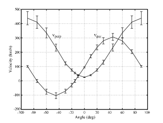
Figure 7.— $V_{\rm par}$ and $V_{\rm perp}$ derived from fitting of an anisotropic model to measurements of ${\bf V_{\rm ISS}}$ for $A_{r}=4$ at various angles for J0737–3039. All fits had the same qu ality. The 95% confidence limits are shown.

In general the ${\bf{\bf V_{A}}}(\phi)^{2}$ model has the form ${\bf{\bf V_{A}}}(\phi)^{2}=A{\rm cos}2\phi+B{\rm sin}2\phi+C{\rm sin}\phi+D{\rm cos}\phi+E$ (again, ignoring terms of the order of the eccentricity). Thus one can fit five independent variables. In the system J1141$-$6545, Ord et al. (2002) fit $S_{\rm ISS}$, $V_{\rm par}$, $V_{\rm perp}$, inclination, and the longitude of periastron. They found a most likely center of mass speed of 115 km s^-1. We tested the effect of anisotropy on this system by fitting the measurements of Ord et al. (2002) and reproducing their result. Then, holding the longitude of periastron constant, we introduced an axial ratio and fit for the remaining parameters. We found a wide range of fits for $1.5<A_{r}<3$, all of which were indistinguishable from the best isotropic fit. All of the fits we tried had greatly reduced $V_{\rm par}$ and $V_{\rm perp}$. For example, with $A_{r}=2.1$, we obtain $\theta=0$, inclination = $75^{{}^{\circ}}$, $V_{\rm par}=20.5$ km s^-1 and $V_{\rm perp}=17.1$ km s^-1.

Although we do not know the value of the anisotropy for J1141$-$6545, this is an important result, because it greatly weakens the case for high transverse velocities in binary systems. Observationally it makes the problem of measuring anisotropy in the ISM of more immediate interest.

6. Conclusions

The cross correlation between the ISS of the two pulsars in the double pulsar system has been measured. It tightly constrains the geometry of the eclipse. We estimate the projected relative distance between the two pulsars at eclipse to be $4000\pm 2000$ km. McLaughlin et al. (2004b) have shown that the eclipse duration varies, depending strongly on B pulse phase. However, if we take the lateral extent of the eclipse to be roughly 18,600 km (derived from the maximum 680 km s^-1 relative velocity of the two pulsars and the average eclipse duration of 27 s), the eclipse must occur at an average radial distance from B of about 9000 km, only 7% of the 130,000 km radius of the light cylinder of B. This is further evidence that the relativistic wind from A has blown away much of the magnetosphere of B.

Our inclination estimate, 0.29${}^{\circ}\pm 0.14^{\circ}$ away from 90^∘, is consistent, within the errors, with the inclination determined from the Shapiro delay. However, the errors on the timing-derived inclination are decreasing significantly with continued observations. If the estimate of inclination determined through the ISS measurements differs from that measured from timing, we may be able to use the measurements of the ISS correlation at different frequencies to estimate the refraction of pulsar A by the magnetosphere of B near the eclipse and determine the density gradient in the magnetosphere. Note that the our inclination estimate is sufficiently small that gravitational lensing may be important (Lai & Rafikov 2004). This effect would bias both the ISS and Shapiro delay estimates of inclination.

The correlations show that the ISS in the direction of the system is anisotropic. When this anisotropy is included in the orbital analysis, the transverse velocity of the center of mass is reduced from $141\pm 8.5$ km s^-1 to $66\pm 15$ km s^-1. We also see that a modest anisotropy in other binary systems, such as J1141$-$6545, can greatly reduce the implied center-of-mass velocity. This decreases the need to invoke large kick velocities and/or high precollapse core masses in double neutron star formation scenarios, as suggested by R04. In fact, as discussed by Piran & Shaviv (2004), the low eccentricity of the system, coupled with its location close to the Galactic plane, suggest a B progenitor mass less than $2~{}M_{\odot}$, and most likely around $1.45~{}M_{\odot}$. This implies a non-standard, possibly white dwarf, progenitor. Willems & Kalogera (2004), who considered the orbital evolution of the system due to gravitational radiation and the orbital dynamics of asymmetric supernova explosions, likewise have difficulty explaining kick velocities of less than 60 km s^-1 given mass ranges derived by assuming a Helium star progenitor and current models of Helium star evolution. Another way we may be able to confirm the low center of mass velocity of the system is through a measurement of the proper motion. Given the closeness of this system, such a measurement should be possible within a year. This will allow us to place better constraints on the kick velocity, the progenitor mass of B and evolutionary scenarios, and will also allow us to test our main conclusion of a significantly anisotropic ISM.

References

- Burgay et al. (2003) Burgay, M. et al. 2003, Nature, 426, 531
- Cordes (1986) Cordes, J. M. 1986, 311, 183
- Cordes & Rickett (1998) Cordes, J. M. & Rickett, B. J. 1998, 507, 846
- Cordes et al. (2004) Cordes, J. M., Rickett, B. J., Stinebring, D. R. & Coles, W. A., ApJ, submitted, astro-ph/0407072
- Desai et al. (1994) Desai, K. M., Gwinn, C. R., & Diamond, P. J. 1994, Nature, 372, 754
- Desai & Fey (2001) Desai, K. M. & Fey, A. L. 2001, ApJS, 133, 395
- Frail et al. (1994) Frail, D. A., Diamond, P. J., Cordes, J. M., & van Langevelde, H. J. 1994, ApJ, 427, L43
- Grall et al. (1997) Grall, R. R. et al. 1997, J. Geophys. Res. 102, 263
- Kaspi et al. (2004) Kaspi, V. M. et al. 2004, ApJ, in press (astro-ph/0401614)
- Lai & Rafikov (2004) Lai, D. & Rafikov, R. R. 2004, ApJ, submitted, (astro-ph/0411726)
-
Lorimer (2001)
Lorimer, D. R. 2001, Arecibo Technical Memo No. 2001–01,
see also
http://www.jb.man.ac.uk/~drl/sigproc - Lyne & Smith (1982) Lyne, A. G. & Smith, F. G. 1982, Nature, 298, 825
- Lyne (1984) Lyne, A. G. 1984, Nature, 310, 300
- Lyne et al. (2004) Lyne, A. G. et al. 2004, Science, 303, 1153
- (15) McLaughlin, M. A. et al. 2004a, ApJ, 613, L57
- (16) McLaughlin, M. A. et al. 2004b, ApJ, 616, L131
- Molbar et al. (1995) Molnar, L.A., Mutel, R.L., Reid, M.J. & Johnston, K.J. 1995, ApJ, 438, 708
- Ord et al. (2002) Ord, S. M., Bailes, M. & van Straten, W. 2002, ApJ, 574, L75
- Piran & Shaviv (2004) Piran, T. & Shaviv, N. J. 2004, (astro-ph/0401553)
- Ramachandran et al. (2004) Ramachandran, R. et al. 2004, ApJ, in press (astro-ph/0404392)
- Ransom et al. (2004) Ransom, S. M. et al. 2004, ApJ, 609, L71
- Rickett (1977) Rickett, B. J., 1977, Ann. Rev. Astron. Astrophys., 479
- Rickett et al. (2002) Rickett, B. J., Kedziora-Chudczer, L., & Jauncey, D. L. 2002, ApJ, 581, 103
- Stinebring et al. (2001) Stinebring, D. R. et al. 2001, ApJ, 549, L97
- Wilkinson et al. (1994) Wilkinson, P.N., Narayan, R. & Spencer, R.E. 1994, MNRAS, 269, 67
- Yusef-Zadeh et al. (1994) Yusef-Zadeh, F., Cotton, W., Wardle, M., Melia, F. & Roberts, D.A. 1994, ApJ, 434, L63