What controls the C iv line profile in active galactic nuclei?

Abstract

The high ionization lines in active galactic nuclei (AGN), such as C iv, tend to be blueshifted with respect to the lower ionization lines, such as H$\rm\beta$, and often show a strong blue excess asymmetry not seen in the low ionization lines. There is accumulating evidence that the H$\rm\beta$ profile is dominated by gravity, and thus provides a useful estimate of the black hole mass in AGN. The shift and asymmetry commonly seen in C iv suggest that non gravitational effects, such as obscuration and radiation pressure, may affect the line profile. We explore the relation between the H$\rm\beta$ and C iv profiles using UV spectra available for 81 of the 87 $z\leq 0.5$ PG quasars in the Boroson & Green (BG92) sample. We find the following: (1) Narrow C iv lines (FWHM $<2000$ km s^-1) are rare ($\sim 2$ per cent occurrence rate) compared to narrow H$\rm\beta$ lines ($\sim 20$ per cent). (2) In most objects where the H$\rm\beta$ FWHM $<4000$ km s^-1 the C iv line is broader than H$\rm\beta$, but the reverse is true when the H$\rm\beta$ FWHM $>4000$ km s^-1. This argues against the view that C iv generally originates closer to the center, compared to H$\rm\beta$. (3) C iv appears to provide a significantly less accurate, and possibly biased estimate of the black hole mass in AGN, compared with H$\rm\beta$. (4) All objects where C iv is strongly blueshifted and asymmetric have a high $L/L_{\rm Edd}$, but the reverse is not true. This suggests that a high $L/L_{\rm Edd}$ is a necessary but not sufficient condition for generating a blueshifted asymmetric C iv emission. (5) We also find indications for dust reddening and scattering in ‘normal’ AGN. In particular, PG quasars with a redder optical-UV continuum slope show weaker C iv emission, stronger C iv absorption, and a higher optical continuum polarization.

1 INTRODUCTION

Systematic differences between the broad low and high ionization emission line profiles in the broad line region (BLR) of active galactic nuclei (AGN) were first noted by Gaskell (1982) and Wilkes (1984; 1986), and later confirmed by various other studies (e.g. Espey et al. 1989; Corbin 1990; Steidel & Sargent 1991; Tytler & Fan 1992; Laor et al. 1994; Wills et al. 1995; Sulentic et al. 1995; Baldwin et al. 1996; Corbin & Boroson 1996; Marziani et al. 1996; McIntosh et al. 1999; Vanden Berk et al. 2001; Richards et al. 2002). The peak of the higher ionization lines (e.g. C iv) tend to be blueshifted with respect to the peak of the low ionization lines (e.g. H$\rm\beta$), and they often show an asymmetric profile with a large excess emission on their blue side, not seen in low ionization lines. These differences suggest that the low and high ionization lines originate in physically distinct components in the BLR, as suggested earlier based on photoionization model fits to the emission line ratios (e.g. Baldwin & Netzer 1978; Collin-Souffrin, Dumont & Tully 1982; Wills, Netzer & Wills 1985; Snedden & Gaskell 2004). The origin of the profile differences is not established yet, but a plausible interpretation is that the blueshift is induced by the combined effect of an outflow and obscuration of the high ionization component versus a virialized unobscured velocity distribution for the low ionization component. The range of amplitudes of the observed profile differences could either be a pure viewing aspect effect in objects which are otherwise intrinsically similar (e.g. Richards et al. 2002), or it could be related to intrinsic differences in the dynamics of the high ionization component (Baldwin et al. 1996; Laor et al. 1997a; Peterson et al. 2000; Leighly 2004a).

There are now good observational indications that the H$\rm\beta$ width is dominated by gravity. Black hole mass, $M_{\rm BH}$, estimates based on the H$\rm\beta$ width give values consistent with the correlation of $M_{\rm BH}$ and host galaxy bulge luminosity and stellar velocity dispersion $\sigma_{*}$ seen in nearby inactive galaxies (Laor 1998; Gebhardt et al. 2000; Ferrarese et al. 2001). The H$\rm\beta$ region is generally not available in objects with $z>1$, and recent studies of $M_{\rm BH}$ in $z>1$ AGN resorted to using the C iv width instead of H$\rm\beta$ (Vestergaard 2002, 2004; Netzer 2003; Corbett et al. 2003; Warner, Hamann & Dietrich 2003, 2004; Dietrich & Hamann 2004). Although efforts were made to calibrate the C iv based $M_{\rm BH}$ estimates using the H$\rm\beta$ results, the differences in line profiles raise the possibility that the C iv profile may be affected by non gravitational forces, which would introduce errors in the $M_{\rm BH}$ estimates.

The purpose of this paper is to obtain observationally based clues for the physical origin of the differences between the C iv and H$\rm\beta$ profiles in AGN. We make a systematic study of the C iv versus H$\rm\beta$ profiles in a nearly (93 per cent) complete sample of low $z$ bright and well studied AGN. We have studied the C iv equivalent width (EW) distribution in this sample in an earlier paper (Baskin & Laor 2004, hereafter BL04). Here we extend the BL04 study by measuring the various C iv profile parameters, and exploring their correlations with the H$\rm\beta$ parameters, as taken from the extensive analysis of Boroson & Green (1992, hereafter BG92). In Section 2 we describe the analysis of the optical and UV spectra, and how the emission line parameters were measured. In Section 3 we describe the results of the correlation analysis and their implications, and the main conclusions are given in Section 4.

2 THE DATA ANALYSIS

2.1 The sample

For the purpose of this analysis we use the BG92 sample which includes the 87 $z\leq 0.5$ AGN from the Bright Quasars Survey (BQS; Schmidt & Green 1983). This sample extends in luminosity from Seyfert galaxies with $\nu L_{\nu}=3.3\times 10^{43}$ erg s^-1 (calculated at rest frame 3000 Å using the continuum fluxes in Neugebauer et al. 1987, assuming $H_{0}=80$ km s^-1 Mpc^-1, $\Omega_{0}=1.0$), to luminous quasars at $\nu L_{\nu}=1.4\times 10^{46}$ erg s^-1. This is a complete and well defined sample, selected based on (blue) color and (point like) morphology, independently of the emission line strengths and profiles. It is also the most thoroughly explored sample of AGN, with a wealth of high quality data at most wave bands, thus making it an optimal sample for comparison of the C iv and H$\rm\beta$ profiles and their relation to other emission properties.

2.2 The optical spectra

The optical observations of the H$\rm\beta$ region of the 87 objects are described in BG92, and were kindly made available to us by T. Boroson (private communication). The rest-frame wavelengths were calculated using redshifts determined from the peak of the [O iii] $\lambda$5007 line (see Table 1), kindly provided to us by T. Boroson. The I Zw 1 Fe ii template, also provided by T. Boroson, was used to subtract the Fe ii lines from the spectra. The template was broadened by convolving with a Gaussian, scaled by multiplying by a constant, and then subtracted from the optical spectrum of each object. The best-fit residual spectrum was searched by eye, while varying the broadening and the absolute flux, based on the criterion of obtaining a featureless continuum between H$\rm\gamma$ at 4340 Å and He ii $\lambda$4686 (BG92). The template was shifted by $\sim 100$ km s^-1 for 19 objects, yielding a better match to the Fe ii emission of those objects.

2.2.1 The absolute flux scale

The BG92 spectra were obtained through a relatively narrow slit which may degrade the absolute spectrophotometric accuracy. BG92 therefore used other spectra (mostly from Neugebauer et al. 1987) to obtain the absolute flux level at rest frame 5500 Å, which they converted to an absolute V magnitude, $M_{\it V}$. We used the cosmology assumed by BG92 ($H_{0}=50$ km s^-1 Mpc^-1, $\Omega_{0}=0.2$), to derive back the observed flux density they used at rest frame 5500 Å. We then measured the corresponding observed flux density in the BG92 spectra. The ratio of the two fluxes defines a correction factor (see Table 1), which we applied to the BG92 spectra in order to get a better spectrophotometric accuracy. Since the BG92 spectra are not corrected for Galactic extinction, while $M_{\it V}$ are corrected, the correction factor also corrects for the Galactic extinction (the differential extinction across BG92 optical spectra is negligible). This process proved essential as otherwise the ‘raw’ BG92 spectra yielded optical to UV spectral slopes which were far too flat (mean $f_{\nu}$ slope of $\sim 0$), while the corrected spectra yielded more plausible values ($\sim-0.5$, Table 1), consistent with the known mean quasar spectral shape.

2.2.2 The H$\rm\beta$ profile

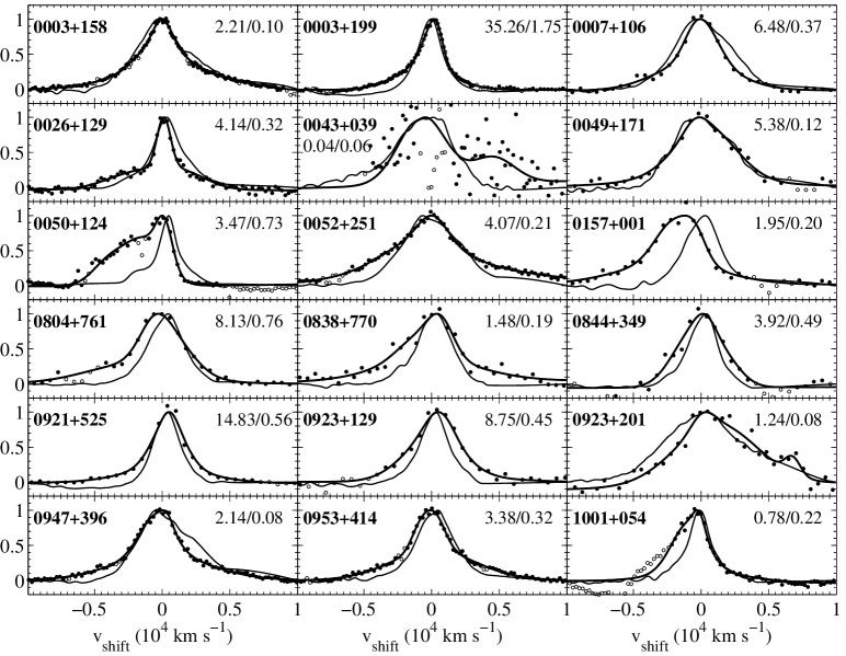
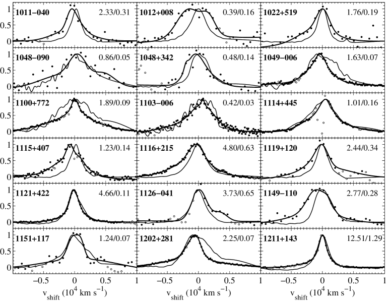
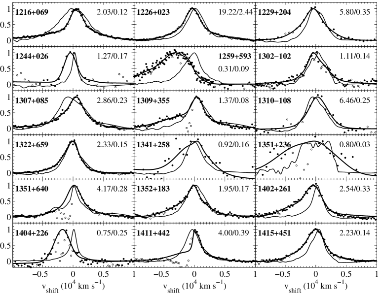
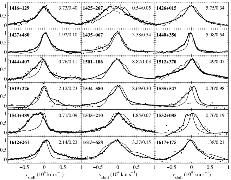
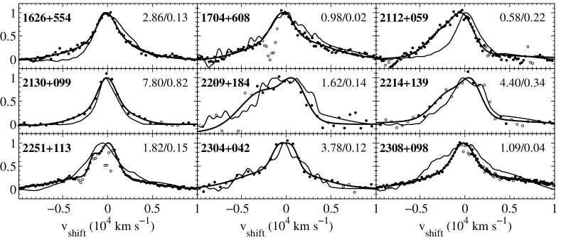
In order to find the BLR H$\rm\beta$ profiles we subtracted the local continuum and the contribution from the narrow line region (NLR). A local power-law continuum was fitted to each spectrum between $\sim 4600$ Å and $\sim 5100$ Å, the continuum flux density at $\lambda$4861 was calculated from the fit (see Table 1), and the power-law fit was subtracted from the spectrum. The [O iii] $\lambda$5007 line profile was used to subtract the narrow component of H$\rm\beta$. No velocity shift was allowed between the NLR components of H$\rm\beta$ and [O iii] $\lambda$5007, and the only free parameter was the narrow component flux. We subtracted the maximum allowed narrow component which does not produce a dip in the H$\rm\beta$ profile, as determined by eye inspection. The narrow component of H$\rm\beta$ generally contributes $<3$ per cent of the total line flux, as noted by BG92, but it is significantly stronger in some of the objects. The EW of the narrow H$\rm\beta$ component is listed for each object in Table 1 (column 17). The H$\rm\beta$ profiles of all objects are presented in Figure 1. However, for the purpose of the correlation analysis we use the H$\rm\beta$ profile parameters as reported by BG92, with the addition of the following two parameters measured here, the continuum flux density and the line flux density at 4861 Å.

2.3 The UV spectra

A complete description of the analysis of the UV spectra is provided in BL04, and is briefly reviewed here. Archival UV spectra of the C iv region are available for 85 of the 87 BG92 objects (PG 1354+213 and PG 2233+134 had no archival UV spectra). The HST archives contain UV spectra of 47 of the objects, which were obtained by the Faint Object Spectrograph (FOS); the UV spectra for the remaining 38 objects with no HST spectra were obtained from the IUE archives (see Table 1). An average spectrum, weighted by the S/N ratio, was calculated when more than one archival spectrum was available. Three of the archival spectra did not have a sufficient S/N to measure the C iv line (of PG 0934+013, PG 1004+130 and PG 1448+273), and in one object C iv is heavily absorbed (PG 1700+518, e.g. Laor & Brandt 2002), leaving a sample of 81 objects for the analysis. We corrected the spectra for Galactic reddening using the E(B$-$V) values from Schlegel, Finkbeiner & Davis (1998, as listed in the NASA/IPAC Extragalactic Database), and the reddening law of Seaton (1979). Absolute wavelength calibration of the FOS spectra was carried out using interstellar absorption lines, when available (see Laor & Brandt 2002).

2.4 The C iv profile

A local power-law continuum was fit to each spectrum between $\sim 1470$ Å and $\sim 1620$ Å, and a narrow ([O iii] like) C iv component was subtracted following the procedure described above for H$\rm\beta$. This narrow component is typically very weak to non detectable, as found in earlier studies (Wills et al. 1993b; Corbin & Boroson 1996; Vestergaard 2002). The subtraction of a narrow C iv component was performed to insure identical analysis of the H$\rm\beta$ and C iv profiles. The resulting broad C iv line emission was fit as a sum of three Gaussians, using the procedure described in Laor et al. (1994, section 3 and the appendix there). Wavelength regions suspected to be affected by intrinsic or Galactic absorption were excluded from the fit (Laor & Brandt 2002). The purpose of the three Gaussians fit is not to decompose the line to possible components, as such a decomposition is not unique, but rather to obtain a smooth realization of the line profile, which is likely to yield more accurate values for the line profile parameters.

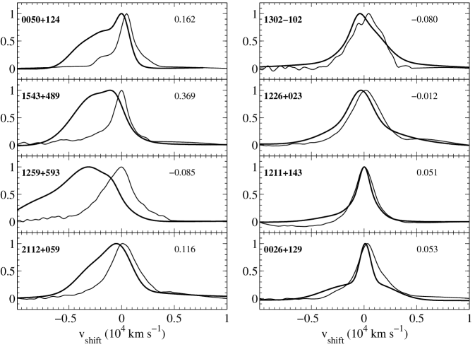
Figure 1 presents all the measured C iv profiles. For each object we show both the smooth fit and the data points. To clarify the presentation we rebinned the UV data, where the HST spectra were rebinned by a factor of four (each four data points were replaced by their average), and the IUE spectra by a factor of two. The H$\rm\beta$ profiles are plots of the data, and again to clarify the presentation we smoothed the H$\rm\beta$ profile by convolving the data with a $\sigma=1.78$ Gaussian (FWHM $\sim 4$ pixels, which produces a negligible line broadening).

Figure 1: A comparison of the H$\rm\beta$ and C iv profiles. The name of the object is indicated in each panel (in bold). The thin line is the smoothed H$\rm\beta$ profile, and the thick line is the fit to the C iv profile (see text). Both profiles are normalized by their peak flux density. The peak flux densities for C iv/H$\rm\beta$ are listed in each panel in units of $10^{-14}$ erg cm^-2 s^-1 Å^-1. The circles indicate the binned C iv data points. Filled circles are data points used in the fitting procedure, and empty circles are data points which were excluded due to possible intrinsic or Galactic absorption (Laor & Brandt 2002). Note the remarkable profile similarity in some objects (e.g. PG 0003+158; PG 1121+422; PG 1416$-$129), and large differences in others (e.g. PG 0157+001; PG 1259+593; PG 1543+489).

Figure 1: — Continued

Figure 1: — Continued

2.5 The measured parameters

The measured C iv profile parameters are listed in Table 1, together with some additional parameters. Specifically, column (2) lists the redshifts determined using the peak of the [O iii] $\lambda$5007 line. Column (3) lists the log of the black hole mass $M_{\rm BH}$ in units of $M_{\sun}$, estimated using $\nu L_{\nu}$(3000Å) and the H$\rm\beta$ FWHM (equation 3 in Laor 1998). Column (4) lists the log of $L/L_{\rm Edd}$ (BL04). Column (5) lists the C iv EW in units of Å (BL04). Column (6) lists the continuum flux density at 1549Å in units of $10^{-15}$ erg cm^-2 s^-1 Å^-1. Column (7) lists the C iv FWHM in units of km s^-1. Column (8) lists the shift of the centroid of C iv at 3/4 maximum from the rest wavelength in units of the FWHM. This is the shift parameter defined by BG92. Negative values indicate a blueshift. The rest wavelength of C iv is taken as 1549.05 Å, which is the mean doublet wavelength for optically thin emission (2:1 flux ratio of the 1548.19 Å/1550.77 Å lines). Column (9) lists the shape parameter for C iv, defined by BG92 as (FW1/4M + FW3/4M)/(2$\times$FWHM). Column (10) lists the line asymmetry parameter, C iv asymmetry, defined by De Roberies (1985) as the shift between the centroids at 1/4 and 3/4 maximum in units of the FWHM. Positive values indicate excess blue wing flux. Column (11) lists the C iv/H$\rm\beta$ line flux ratio, R $f_{\rm line}$ (throughout this paper the prefix ‘R’ indicates the ratio of a variable to that of H$\rm\beta$). The H$\rm\beta$ line flux was calculated using the H$\rm\beta$ EW (BG92) and continuum flux density at 4861Å measured here. Column (12) lists the log of R C iv FWHM, calculated using the H$\rm\beta$ FWHM values from BG92 and the C iv FWHM values in column (7). Column (13) lists the ratio of the C iv to H$\rm\beta$ line flux density at $v_{\rm shift}=0$. Column (14) lists the continuum flux density at 4861Å in units of $10^{-15}$ erg cm^-2 s^-1 Å^-1. Column (15) lists the optical to UV slope $\alpha_{\rm o,UV}$, measured between 4861 Å and 1549 Å using $f_{\nu}$. Columns (16) and (17) list the EW of the narrow, [O iii] like, component of C iv and H$\rm\beta$, respectively, in units of Å. Finally, column (18) lists the correction factor for the flux densities of the optical spectra (Section 2.2.1).

Table 1: Emission-line and continuum properties.

Object	$z$	$M_{\rm BH}$	$L/L_{\rm Edd}$	C iv									$f_{\rm cont}$	$\alpha_{\rm o,UV}$	N.C. EW		corre-
				EW${}^{\ref{fn:1a}}$	$f_{\rm cont}$	FWHM	shift	shape	asymm	R $f_{\rm line}$	R FWHM	R $f$(0)	(4861)		C iv	H$\rm\beta$	ction
(1)	(2)	(3)	(4)	(5)	(6)	(7)	(8)	(9)	(10)	(11)	(12)	(13)	(14)	(15)	(16)	(17)	(18)
0003+158	$0.4505$	$9.055$	$-0.358$	$63.5$	$9.7$	$3490$	$-$0.007	$1.255$	$-$0.067	$4.85$	$-0.135$	$20.79$	$1.39$	$-0.30$	$1.3$	$1.8$	$1.28$
0003+199	$0.0260$	$7.220$	$-0.342$	$60.1$	$87.9$	$2090$	$0.049$	$1.181$	$0.202$	$5.21$	$0.106$	$17.64$	$10.66$	$-0.16$	$1.4$	$4.7$	$1.20$
0007+106	$0.0893$	$8.561$	$-0.972$	$59$	$26.2$	$3550$	$-$0.004	$1.151$	$0.053$	$4.54$	$-0.158$	$16.69$	$3.38$	$-0.21$	—	$4.1$	$1.42$
0026+129	$0.1452$	$7.833$	$0.053$	$19.3$	$35.9$	$1600$	$0.075$	$1.674$	$0.151$	$3.41$	$-0.067$	$12.64$	$3.12$	$0.14$	$0.3$	$2.9$	$2.01$
0043+039	$0.3859$	$8.952$	$-0.648$	$5.4$	$2.1$	$4490$	$-$0.142	$1.380$	$-$0.411	$0.14$	$-0.072$	$0.57$	$0.84$	$-1.22$	—	—	$1.29$
0049+171	$0.0643$	$8.146$	$-1.437$	$203$	$7.7$	$4980$	$0.021$	$1.053$	$-$0.025	$12.49$	$-0.023$	$37.49$	$0.92$	$-0.14$	$0.4$	$13.7$	$1.80$
0050+124	$0.0587$	$7.238$	$0.162$	$29.9$	$25.5$	$4430$	$-$0.040	$0.864$	$0.381$	$2.45$	$0.553$	$6.39$	$6.09$	$-0.75$	$1.9$	$7.0$	$1.45$
0052+251	$0.1544$	$8.745$	$-0.822$	$119.0$	$14.6$	$5610$	$-$0.019	$1.168$	$0.024$	$7.28$	$0.033$	$17.62$	$2.75$	$-0.54$	$0.5$	$3.7$	$1.59$
0157+001	$0.1632$	$8.006$	$-0.261$	$43$	$12.7$	$4430$	$-$0.344	$1.090$	$0.105$	$2.74$	$0.255$	$6.08$	$2.54$	$-0.59$	$2.1$	$8.6$	$2.07$
0804+761	$0.1005$	$8.352$	$-0.300$	$45$	$48.6$	$4120$	$-$0.051	$1.146$	$0.067$	$4.09$	$0.128$	$10.91$	$4.51$	$0.08$	$0.8$	$3.6$	$1.44$
0838+770	$0.1318$	$7.992$	$-0.493$	$50$	$8.1$	$4370$	$0.045$	$1.083$	$0.140$	$2.79$	$0.195$	$6.93$	$1.43$	$-0.48$	$0.7$	$3.3$	$2.43$
0844+349	$0.0644$	$7.759$	$-0.479$	$28$	$31.0$	$3870$	$0.013$	$1.034$	$0.006$	$2.91$	$0.204$	$8.45$	$3.97$	$-0.20$	$0.7$	$2.1$	$2.12$
0921+525	$0.0352$	$7.206$	$-0.802$	$186$	$15.7$	$2940$	$0.166$	$1.095$	$0.021$	$7.91$	$0.142$	$24.06$	$2.54$	$-0.41$	$2.9$	$10.4$	$2.47$
0923+129	$0.0287$	$7.233$	$-0.665$	$93$	$22.6$	$3900$	$0.112$	$1.086$	$0.055$	$6.90$	$0.292$	$17.53$	$4.03$	$-0.49$	$1.0$	$6.4$	$2.88$
0923+201	$0.1929$	$9.094$	$-1.134$	$28$	$17.3$	$6200$	$0.128$	$1.159$	$-$0.172	$2.87$	$-0.089$	$17.29$	$1.06$	$0.44$	$1.1$	$0.9$	$0.89$
0947+396	$0.2059$	$8.530$	$-0.909$	$55$	$10.2$	$3650$	$-$0.073	$1.204$	$-$0.020	$5.98$	$-0.121$	$26.82$	$0.85$	$0.18$	$0.8$	$1.8$	$1.18$
0953+414	$0.2341$	$8.488$	$-0.196$	$54.9$	$14.9$	$3250$	$-$0.039	$1.304$	$-$0.074	$2.36$	$0.016$	$10.67$	$2.22$	$-0.34$	$1.4$	$4.3$	$1.55$
1001+054	$0.1610$	$7.645$	$-0.020$	$34.9$	$4.3$	$2920$	$-$0.200	$1.074$	$0.069$	$1.37$	$0.225$	$3.20$	$1.22$	$-0.90$	$0.9$	$2.5$	$2.53$
1011$-$040	$0.0584$	$7.190$	$-0.146$	$25$	$19.4$	$2960$	$-$0.114	$1.170$	$-$0.032	$3.76$	$0.313$	$7.18$	$2.86$	$-0.33$	$0.3$	$2.9$	$2.64$
1012+008	$0.1865$	$8.069$	$-0.320$	$23$	$5.8$	$6500$	$-$0.076	$1.018$	$0.031$	$0.82$	$0.391$	$2.11$	$1.57$	$-0.86$	$2.9$	$5.8$	$2.00$
1022+519	$0.0449$	$6.940$	$-0.600$	$38$	$13.7$	$3550$	$-$0.011	$1.245$	$0.212$	$4.99$	$0.341$	$9.64$	$1.52$	$-0.08$	$1.1$	$3.4$	$1.00$
1048$-$090	$0.3461$	$9.022$	$-0.679$	$91$	$4.0$	$5190$	$0.081$	$1.367$	$-$0.046	$4.15$	$-0.034$	$16.37$	$1.07$	$-0.86$	—	$1.6$	$0.87$
1048+342	$0.1667$	$8.241$	$-0.687$	$46$	$2.4$	$4060$	$-$0.141	$1.076$	$-$0.159	$0.38$	$0.053$	$3.10$	$1.25$	$-1.43$	$1.9$	$2.4$	$4.06$
1049$-$006	$0.3596$	$8.989$	$-0.630$	$67.0$	$6.7$	$3660$	$-$0.119	$1.136$	$0.051$	$4.23$	$-0.165$	$23.84$	$0.99$	$-0.34$	$0.1$	$4.7$	$3.25$
1100+772	$0.3115$	$9.112$	$-0.749$	$84.0$	$7.0$	$3610$	$0.019$	$1.451$	$0.106$	$4.06$	$-0.232$	$19.58$	$1.61$	$-0.71$	$0.8$	$3.8$	$1.75$
1103$-$006	$0.4232$	$9.132$	$-0.737$	$37.2$	$3.3$	$4370$	$0.120$	$1.087$	$0.104$	$2.54$	$-0.151$	$10.25$	$0.60$	$-0.52$	$1.1$	$2.7$	$1.61$
1114+445	$0.1438$	$8.415$	$-0.927$	$55.0$	$4.9$	$3830$	$0.129$	$1.216$	$0.084$	$1.46$	$-0.077$	$5.96$	$1.84$	$-1.15$	—	$2.0$	$2.18$
1115+407	$0.1542$	$7.505$	$-0.139$	$25.9$	$11.1$	$3600$	$-$0.185	$1.122$	$0.041$	$4.54$	$0.320$	$7.49$	$1.04$	$0.07$	—	$5.1$	$2.02$
1116+215	$0.1765$	$8.425$	$-0.139$	$40.5$	$35.3$	$4280$	$-$0.108	$1.213$	$0.085$	$2.01$	$0.166$	$7.10$	$4.07$	$-0.11$	—	$4.5$	$1.35$
1119+120	$0.0500$	$7.280$	$-0.462$	$29$	$26.2$	$3660$	$-$0.057	$1.286$	$-$0.011	$4.55$	$0.304$	$7.33$	$3.36$	$-0.20$	$0.4$	$2.6$	$1.22$
1121+422	$0.2248$	$7.856$	$-0.232$	$41.7$	$15.9$	$2000$	$-$0.046	$1.160$	$-$0.035	$10.47$	$-0.046$	$43.18$	$0.71$	$0.71$	—	$3.3$	$0.62$
1126$-$041	$0.0601$	$7.598$	$-0.434$	$30$	$23.3$	$3860$	$0.037$	$1.000$	$-$0.242	$2.01$	$0.254$	$5.52$	$3.45$	$-0.33$	$1.1$	$3.2$	$2.26$
1149$-$110	$0.0489$	$7.729$	$-0.916$	$82$	$11.1$	$4920$	$-$0.123	$1.073$	$0.058$	$3.65$	$0.206$	$8.67$	$2.12$	$-0.55$	$0.8$	$4.1$	$1.21$
1151+117	$0.1759$	$8.435$	$-0.801$	$26.6$	$12.8$	$3170$	$0.064$	$1.472$	$-$0.205	$2.98$	$-0.133$	$17.06$	$0.90$	$0.33$	$1.1$	$1.3$	$0.75$
1202+281	$0.1654$	$8.462$	$-1.053$	$290.0$	$2.0$	$3190$	$-$0.216	$1.156$	$0.092$	$4.49$	$-0.200$	$26.51$	$0.90$	$-1.31$	$4.6$	$5.3$	$0.98$
1211+143	$0.0810$	$7.831$	$0.051$	$55.7$	$29.4$	$1690$	$0.012$	$1.224$	$0.068$	$2.35$	$-0.043$	$8.96$	$8.32$	$-0.90$	$0.9$	$3.1$	$2.21$
1216+069	$0.3318$	$8.954$	$-0.609$	$64.5$	$8.9$	$3120$	$0.180$	$1.354$	$0.033$	$3.69$	$-0.221$	$14.46$	$1.78$	$-0.60$	$1.1$	$1.4$	$0.58$
1226+023	$0.1575$	$8.876$	$-0.012$	$23.0$	$211.0$	$3430$	$-$0.085	$1.222$	$-$0.004	$1.51$	$-0.011$	$7.40$	$28.41$	$-0.25$	—	$1.2$	$2.69$
1229+204	$0.0640$	$8.004$	$-0.804$	$48$	$29.9$	$4010$	$-$0.103	$1.134$	$0.005$	$3.99$	$0.077$	$14.86$	$3.40$	$-0.10$	—	$1.8$	$1.15$
1244+026	$0.0480$	$6.614$	$0.235$	$17$	$10.1$	$2410$	$-$0.175	$1.034$	$-$0.024	$2.27$	$0.463$	$7.81$	$1.82$	$-0.50$	$1.1$	$7.8$	$2.45$
1259+593	$0.4770$	$8.738$	$-0.085$	$15.3$	$7.9$	$6920$	$-$0.437	$1.071$	$0.215$	$1.97$	$0.310$	$1.58$	$1.00$	$-0.19$	—	—	$1.58$
1302$-$102	$0.2783$	$8.749$	$-0.080$	$13.1$	$20.8$	$3580$	$-$0.061	$1.077$	$-$0.101	$2.85$	$0.022$	$9.18$	$3.41$	$-0.42$	$0.2$	$2.2$	$3.43$
1307+085	$0.1545$	$8.541$	$-0.651$	$71.2$	$11.0$	$3680$	$0.129$	$1.190$	$0.119$	$2.71$	$-0.057$	$11.66$	$2.26$	$-0.62$	$0.5$	$3.0$	$1.02$
1309+355	$0.1825$	$8.155$	$-0.421$	$33.5$	$11.3$	$3320$	$0.117$	$1.484$	$0.421$	$4.49$	$0.053$	$15.41$	$1.65$	$-0.32$	$0.6$	$2.5$	$1.39$
1310$-$108	$0.0343$	$7.759$	$-1.183$	$78$	$18.8$	$3790$	$0.092$	$1.051$	$-$0.011	$5.66$	$0.019$	$23.00$	$2.63$	$-0.28$	$1.2$	$7.0$	$1.70$
1322+659	$0.1676$	$8.076$	$-0.409$	$52.6$	$8.5$	$2990$	$-$0.055	$1.103$	$0.089$	$4.27$	$0.030$	$15.00$	$1.36$	$-0.40$	—	$1.0$	$1.73$
1341+258	$0.0864$	$7.878$	$-0.756$	$62$	$4.8$	$5460$	$-$0.017	$1.040$	$0.024$	$1.82$	$0.254$	$5.53$	$1.37$	$-0.90$	$2.1$	$1.8$	$1.06$
1351+236	$0.0553$	$8.216$	$-1.748$	$101$	$4.5$	$10250$	$-$0.105	$1.004$	$0.028$	$8.80$	$0.195$	$22.92$	$2.28$	$-1.40$	—	$2.5$	$1.80$
1351+640	$0.0880$	$8.656$	$-1.058$	$43.3$	$20.4$	$3310$	$0.052$	$1.098$	$0.004$	$3.20$	$-0.233$	$12.67$	$4.76$	$-0.73$	—	$3.5$	$1.86$
1352+183	$0.1508$	$8.299$	$-0.629$	$45.1$	$10.3$	$3350$	$-$0.049	$1.252$	$0.131$	$2.71$	$-0.031$	$10.21$	$1.29$	$-0.18$	—	$1.4$	$2.23$
1402+261	$0.1643$	$7.845$	$0.018$	$30.3$	$25.0$	$4090$	$-$0.121	$1.232$	$0.282$	$6.31$	$0.330$	$7.76$	$1.58$	$0.41$	—	—	$3.23$
1404+226	$0.0978$	$6.713$	$0.232$	$23.3$	$6.2$	$3260$	$-$0.538	$0.991$	$-$0.002	$2.35$	$0.569$	$1.19$	$1.13$	$-0.51$	—	—	$0.99$
1411+442	$0.0897$	$7.874$	$-0.535$	$56.9$	$11.5$	$3080$	$0.088$	$0.814$	$0.137$	$2.32$	$0.062$	$10.35$	$2.66$	$-0.72$	—	$2.1$	$1.31$
1415+451	$0.1133$	$7.797$	$-0.579$	$57.3$	$9.5$	$3730$	$-$0.016	$1.151$	$0.118$	$7.67$	$0.154$	$18.63$	$1.22$	$-0.21$	—	$0.1$	$1.33$
1416$-$129	$0.1292$	$9.002$	$-0.845$	$168.1$	$6.2$	$4090$	$0.001$	$1.139$	$0.083$	$1.65$	$-0.174$	$7.65$	$3.65$	$-1.53$	—	$3.2$	$6.04$
1425+267	$0.3635$	$9.317$	$-1.280$	$64.8$	$4.1$	$8620$	$0.161$	$0.606$	$0.276$	$2.37$	$-0.038$	$9.76$	$1.20$	$-0.93$	—	$3.5$	$1.28$
1426+015	$0.0863$	$8.921$	$-1.117$	$32$	$60.7$	$4910$	$-$0.021	$1.192$	$0.070$	$4.26$	$-0.143$	$16.77$	$5.23$	$0.14$	$0.4$	$0.6$	$1.71$
1427+480	$0.2203$	$7.978$	$-0.344$	$53.2$	$7.0$	$2880$	$0.094$	$1.159$	$-$0.055	$4.69$	$0.054$	$17.78$	$0.58$	$0.18$	$1.1$	$3.3$	$1.51$
1435$-$067	$0.1288$	$8.300$	$-0.412$	$39$	$21.1$	$3750$	$-$0.051	$1.125$	$0.082$	$1.77$	$0.071$	$6.04$	$3.30$	$-0.38$	—	$1.3$	$2.91$
1440+356	$0.0777$	$7.335$	$-0.013$	$30.1$	$29.4$	$2530$	$-$0.125	$1.193$	$0.211$	$4.61$	$0.241$	$8.91$	$3.00$	$-0.01$	$0.6$	$4.5$	$1.35$
1444+407	$0.2676$	$8.158$	$-0.122$	$17.9$	$11.6$	$4340$	$-$0.143	$1.081$	$0.133$	$3.03$	$0.243$	$6.08$	$0.95$	$0.19$	—	—	$0.84$
1501+106	$0.0365$	$8.482$	$-1.172$	$64$	$44.2$	$4710$	$-$0.058	$1.163$	$0.085$	$2.12$	$-0.065$	$8.12$	$9.68$	$-0.67$	$0.2$	$5.1$	$2.20$

Table 1: — Continued

Object	$z$	$M_{\rm BH}$	$L/L_{\rm Edd}$	C iv									$f_{\rm cont}$	$\alpha_{\rm o,UV}$	N.C. EW		corre-
				EW	$f_{\rm cont}$	FWHM	shift	shape	asymm	R $f_{\rm line}$	R FWHM	R $f$(0)	(4861)		C iv	H$\rm\beta$	ction
(1)	(2)	(3)	(4)	(5)	(6)	(7)	(8)	(9)	(10)	(11)	(12)	(13)	(14)	(15)	(16)	(17)	(18)
1512+370	$0.3713$	$9.168$	$-0.867$	$84.3$	$6.7$	$4450$	$0.021$	$1.399$	$0.186$	$4.79$	$-0.185$	$20.36$	$0.96$	$-0.31$	$0.5$	$5.9$	$2.45$
1519+226	$0.1357$	$7.777$	$-0.311$	$68$	$7.3$	$3080$	$-$0.052	$1.400$	$-$0.153	$4.54$	$0.141$	$9.37$	$1.05$	$-0.30$	—	$5.6$	$2.35$
1534+580	$0.0305$	$8.047$	$-1.565$	$79$	$29.7$	$4010$	$0.015$	$1.141$	$0.153$	$6.12$	$-0.125$	$24.89$	$3.96$	$-0.24$	—	$5.4$	$1.37$
1535+547	$0.0389$	$7.010$	$-0.373$	$27.6$	$5.1$	$3690$	$0.132$	$0.986$	$0.233$	$0.29$	$0.396$	$0.59$	$4.42$	$-1.87$	$1.6$	$4.0$	$1.72$
1543+489	$0.4009$	$7.844$	$0.369$	$25.6$	$8.7$	$5330$	$-$0.364	$1.020$	$0.079$	$5.82$	$0.533$	$5.68$	$0.48$	$0.53$	—	—	$1.05$
1545+210	$0.2643$	$9.165$	$-0.925$	$90.5$	$6.7$	$4530$	$0.041$	$1.212$	$-$0.007	$4.23$	$-0.191$	$23.50$	$1.48$	$-0.69$	$1.2$	$2.7$	$1.61$
1552+085	$0.1191$	$7.364$	$0.040$	$47$	$5.5$	$4900$	$-$0.005	$1.130$	$0.040$	$3.51$	$0.535$	$4.23$	$1.59$	$-0.91$	$1.4$	$2.7$	$1.11$
1612+261	$0.1308$	$7.913$	$-0.395$	$94.6$	$6.5$	$3810$	$0.114$	$1.266$	$-$0.118	$2.53$	$0.180$	$7.60$	$1.39$	$-0.64$	—	$12.9$	$1.12$
1613+658	$0.1291$	$8.953$	$-1.457$	$54$	$22.6$	$5730$	$-$0.104	$1.084$	$-$0.056	$4.76$	$-0.168$	$19.69$	$2.35$	$-0.02$	$0.1$	$1.3$	$1.14$
1617+175	$0.1137$	$8.729$	$-0.880$	$34$	$11.9$	$4500$	$-$0.076	$1.155$	$0.013$	$1.48$	$-0.074$	$6.60$	$2.38$	$-0.59$	—	$1.1$	$2.37$
1626+554	$0.1317$	$8.371$	$-0.940$	$45.6$	$16.6$	$3510$	$-$0.025	$1.234$	$0.002$	$4.65$	$-0.107$	$22.12$	$1.14$	$0.34$	—	$0.5$	$0.92$
1704+608	$0.3721$	$9.198$	$-0.772$	$34.8$	$9.4$	$4340$	$-$0.086	$1.326$	$-$0.155	$8.25$	$-0.180$	$46.54$	$1.42$	$-0.35$	$0.3$	$2.7$	$1.16$
2112+059	$0.4597$	$8.834$	$0.116$	$25.5$	$6.4$	$4790$	$-$0.159	$0.999$	$0.141$	$0.90$	$0.176$	$2.33$	$1.49$	$-0.73$	—	—	$1.74$
2130+099	$0.0631$	$7.805$	$-0.367$	$47$	$35.0$	$3120$	$-$0.020	$1.154$	$-$0.007	$3.38$	$0.127$	$9.47$	$4.51$	$-0.21$	$0.2$	$1.5$	$1.07$
2209+184	$0.0697$	$8.601$	$-1.353$	$54$	$12.4$	$7420$	$-$0.091	$0.970$	$0.116$	$2.77$	$0.058$	$11.03$	$2.11$	$-0.45$	$3.6$	$2.7$	$2.95$
2214+139	$0.0657$	$8.308$	$-1.027$	$45$	$28.1$	$5200$	$-$0.001	$0.978$	$0.150$	$2.80$	$0.058$	$11.80$	$4.21$	$-0.34$	$2.1$	$0.6$	$0.87$
2251+113	$0.3255$	$8.816$	$-0.363$	$66.0$	$7.7$	$3580$	$-$0.093	$1.209$	$0.061$	$3.49$	$-0.065$	$13.12$	$1.78$	$-0.72$	—	$2.1$	$0.93$
2304+042	$0.0426$	$8.320$	$-1.633$	$176$	$6.8$	$4040$	$-$0.044	$1.381$	$0.146$	$5.55$	$-0.206$	$27.08$	$2.19$	$-1.01$	$6.3$	$0.6$	$1.04$
2308+098	$0.4336$	$9.372$	$-0.936$	$81.5$	$5.1$	$3970$	$-$0.036	$1.342$	$-$0.023	$5.26$	$-0.303$	$23.22$	$0.87$	$-0.46$	—	$1.6$	$1.61$

3 RESULTS & DISCUSSION

3.1 The C iv versus H$\rm\beta$ profile parameters

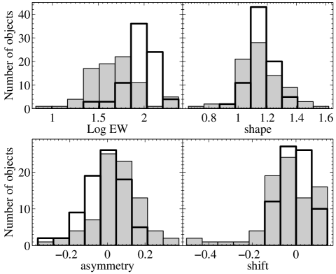
Figure 2 compares the distribution of the EW and the profile parameters: shape, asymmetry, and shift for C iv and H$\rm\beta$. The C iv line shows a broader distribution in all parameters. In particular, the C iv EW (in Å) ranges from 5 to 290, with a mean and dispersion of $59\pm 45$, while H$\rm\beta$ EW ranges from 23 to 230 with a mean and dispersion of $99\pm 37$, i.e. the dispersion/mean ratio in C iv is twice as large as in H$\rm\beta$. The asymmetry parameter distribution of H$\rm\beta$ shows a small excess of negative values, which correspond to red asymmetric profiles (i.e. excess flux on the red wing), while C iv shows a large excess of blue asymmetric profiles. Similarly, the shift parameter in C iv extends to a blue shift of $-0.538$, while in H$\rm\beta$ the maximum blue shift is only $-0.135$ (see similar result in fig. 3 of Sulentic, Marziani & Dultzin-Hacyan 2000). In both lines the maximum shift to the red is small. This confirms the various earlier literature results on the systematic differences between the high and low ionization line profiles (Section 1).

Figure 2: The distributions of $\log$ EW, shape, asymmetry and shift of the H$\rm\beta$ line (transparent) and the C iv line (gray) profiles. Note the larger range in EW and shape parameter values for C iv, its tendency to show blue excess flux asymmetry (positive asymmetry parameter), and the ‘tail’ of objects with large shifts to the blue (negative shift parameter).

3.2 The C iv versus H$\rm\beta$ FWHM

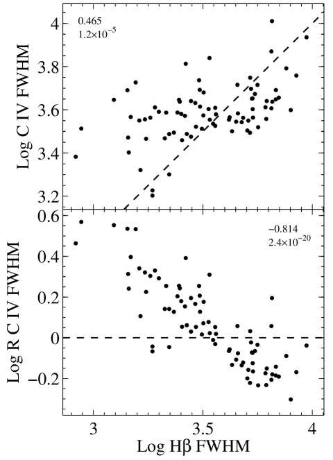
Figure 3 presents the C iv FWHM versus H$\rm\beta$ FWHM. The two lines show quite different distributions of line widths. The C iv line shows a smaller relative range of FWHM (1600-10,250 km s^-1, a ratio of 6.4) compared to H$\rm\beta$ (830-9400 km s^-1, ratio of 11.3), with most objects having FWHM in the range of 3000-5000 km s^-1, compared to a rather even distribution in the range 1500-8000 km s^-1 for H$\rm\beta$. Furthermore, there is a distinct lack of AGN with a narrow C iv. About 21 per cent (17/81) of our objects qualify as ‘narrow line’ AGN based on H$\rm\beta$, i.e. have FWHM $<$ 2000 km s^-1, but only 2.5 per cent (2/81) of the objects have a C iv FWHM $<$ 2000 km s^-1.

Figure 3 (upper panel) shows that although there is a significant correlation between the C iv and H$\rm\beta$ FWHM, as found in earlier studies (Corbin 1991; Corbin & Boroson 1996; Marziani et al. 1996), the scatter in the correlation is large. Most importantly, the scatter is not random but rather shows a systematic trend. Fig. 3 (lower panel) shows the ratio of C iv/H$\rm\beta$ FWHM as a function of H$\rm\beta$ FWHM. In most ($\sim 90$ per cent) objects with H$\rm\beta$ FWHM $<$ 4000 km s^-1 the C iv line is broader than H$\rm\beta$, while in most objects where H$\rm\beta$ FWHM $>$ 4000 km s^-1 the C iv line is narrower than H$\rm\beta$. A similar effect is seen in fig. 7 of Shemmer et al. (2004), where they plot the distribution of the C iv FWHM versus H$\rm\beta$ FWHM for a sample 82 quasars, all at a relatively high redshift ($2<z<3.5$) compared to our sample ($z<0.5$). This similarity is noteworthy given the large difference in redshift and maximum luminosities of the two samples (a similar effect is also seen in the low redshift sample of Corbin & Boroson 1996, fig.7 there).

A commonly accepted view is that the C iv line tends to be broader than H$\rm\beta$ (e.g. fig. 4 in Warner et al. 2003), which is consistent with the smaller emission radius indicated in some reverberation studies (see Section 3.3). However, this appears not to hold in most of the H$\rm\beta$ FWHM $>$ 4000 km s^-1 objects, where C iv is narrower than H$\rm\beta$. A prominent example of such a reverese behaviour is found in the subclass of double peaked Balmer line AGN, where H$\rm\beta$ is often broader than C iv (Halpern et al. 1996).

The systematic differences between the H$\rm\beta$ and C iv profiles raise the concern, can the C iv FWHM replace the H$\rm\beta$ FWHM as a comparable accuracy tool for estimating $M_{\rm BH}$?

Figure 3: Upper panel: the C iv FWHM versus H$\rm\beta$ FWHM correlation. The dashed line marks a 1:1 relation. Lower panel: the relation between C iv FWHM/H$\rm\beta$ FWHM ratio and the H$\rm\beta$ FWHM. The values of $r_{\rm S}$ and Pr are indicated. Note that in nearly all objects where H$\rm\beta$ FWHM $<4000$ km s^-1 C iv is broader than H$\rm\beta$, while in most objects where H$\rm\beta$ FWHM $>4000$ km s^-1 C iv is narrower than H$\rm\beta$.

3.3 The C iv based $M_{\rm BH}$ estimates

Current studies which utilize the C iv FWHM to estimate $M_{\rm BH}$ (Vestergaard 2002; Corbett et al. 2003; Warner et al. 2003, 2004; Dietrich & Hamann 2004) assume the same dependence of $M_{\rm BH}$ on luminosity and line width as used in the H$\rm\beta$ based $M_{\rm BH}$ estimates (e.g. Kaspi et al. 2000). Intercalibration of the two methods in the studies above yields a constant correction factor, which corresponds to a mean C iv emission radius in the BLR of about half the H$\rm\beta$ emission radius, consistent with reverberation results in some nearby AGN (Korista et al. 1995; Onken & Peterson 2002). However, the systematic trend in the C iv/H$\rm\beta$ FWHM ratio shown in Fig. 3 indicates that the above C iv based $M_{\rm BH}$ estimates will be biased. Since $M_{\rm BH}$ $\propto$ FWHM(line)², the C iv based $M_{\rm BH}$ estimates in objects with H$\rm\beta$ FWHM $<$ 4000 km s^-1 will be too high by a factor of typically 3-4, and up to a factor of 10 in the extreme cases. Similarly, in objects with H$\rm\beta$ FWHM $>$ 4000 km s^-1 the above C iv based $M_{\rm BH}$ estimates will be too low by the same factors (see Section 3.5).

As Fig. 3 (upper panel) shows, the C iv FWHM is only weakly dependent on the H$\rm\beta$ FWHM, which indicates that the above bias cannot be reliably corrected based on the C iv FWHM, e.g. an AGN with C iv FWHM = 4000 km s^-1 can have an H$\rm\beta$ FWHM anywhere from  1500 km s^-1 to  7000 km s^-1 with about the same probability. However, indirect correlations mentioned below (Section 3.5) may allow somewhat more accurate estimates of the likely H$\rm\beta$ FWHM for a given C iv FWHM.

An additional, less direct, indication for the lower accuracy of the C iv $M_{\rm BH}$ estimate is provided by the Baldwin relation. BL04 have shown that the Baldwin relation for C iv appears to be induced by a significantly tighter relation between the C iv EW and $L/L_{\rm Edd}$ ($r_{\rm S}$ $=-0.581$, Figure 4, left panel). We have repeated this analysis with $L/L_{\rm Edd}$ estimated using the C iv based expression for $M_{\rm BH}$ provided by Vestergaard (2002) . No significant correlation is present between the C iv EW and $L/L_{\rm Edd}$ derived using the Vestergaard relation ($r_{\rm S}$ $=-0.205$, Fig. 4, middle panel), which most likely results from the large scatter present in the C iv based $M_{\rm BH}$ estimates. A qualitatively similar result was found by Shemmer et al. (2004), where they find a significant correlation between the BLR metalicity and $L/L_{\rm Edd}$ in their $2<z<3.5$ sample, when $M_{\rm BH}$ is estimated using H$\rm\beta$, but a significantly lower correlation when C iv is used to infer $M_{\rm BH}$ (figs. 5 & 8 there).

Figure 4: An indirect indication for the accuracy of the C iv based $M_{\rm BH}$ estimate ($r_{\rm S}$ and Pr are indicated in each panel). Left panel: the correlation of the C iv EW with $L/L_{\rm Edd}$ estimated based on the H$\rm\beta$ FWHM and $\nu L_{\nu}$(3000 Å) (taken from BL04). Middle panel: the same correlation where $L/L_{\rm Edd}$ is estimated using the Vestergaard (2002) relation for $M_{\rm BH}$, based on the C iv FWHM and the UV luminosity. Note the significant drop in $r_{\rm S}$ compared to the H$\rm\beta$ based estimate. Right panel: the linear combination of log[$\nu L_{\nu}$(1549 Å)] and log(C iv FWHM) which gives the largest $r_{\rm S}$. Note that the improved $r_{\rm S}$ is still not significant.

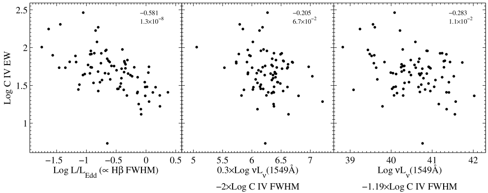
The C iv line may follow a different radius luminosity relation than assumed by Vestergaard. To allow for that we looked for the strongest correlation of log C iv EW with a general linear combination of the form log [$\nu L_{\nu}$(1549 Å)] $+a\log$(C iv FWHM), where $a$ is a free parameter. The strongest correlation we find is $r_{\rm S}$ $=-0.283$ at $a=-1.19$ (Fig. 4, right panel). This correlation is still much weaker than the correlation with $L/L_{\rm Edd}$ estimated based on H$\rm\beta$. This indicates that the scatter seen in the C iv versus H$\rm\beta$ FWHM relation (Fig. 3) is probably not just due to a different radius versus luminosity power law relation for the C iv emitting region (e.g. if $M_{\rm BH}$ $\propto$ C iv FWHM² then $a=-1.19$ implies $R_{\rm BLR}\propto L^{1.68}$ for C iv, which appears unlikely; the alternative option of maintaining $R_{\rm BLR}\propto L^{0.5}$ for C iv would require $M_{\rm BH}$ $\propto$ C iv FWHM^0.6 which appears even less plausible). What is it then that determines the C iv profile?

3.4 The correlation analysis

To obtain clues for the effects which may control the C iv profile, and in particular the differences between the C iv and H$\rm\beta$ profiles, we carried out an extensive correlation analysis, as described below. We use the Spearman rank-order correlation coefficient, which tests for any monotonic relation, rather than the Pearson correlation coefficient, which tests the significance of a linear relation only.

Table 2 presents the correlation matrix. Rows are present for all the items from Table 1 (except the narrow component EW of C iv and H$\rm\beta$), all the optical emission line parameters from BG92 (see BG92 for definitions), the values of the optical to X-ray slope (3000 Å to 2 keV) $\alpha_{\rm ox}$ from Brandt, Laor & Wills (2000) and Laor & Brandt (2002), $\nu L_{\nu}$(3000 Å), $M_{\rm BH}$ and $L/L_{\rm Edd}$ (see above), $\alpha_{\rm x}$, measured at 0.2-2 keV (Wang et al. 1996; Laor et al. 1997b), the optical continuum slope $\alpha_{\rm o}$ from Neugebauer et al. (1987, table 5 there), the degree of broadband optical continuum polarization (3200-8600 Å; Berriman et al. 1990, table 1 there), and the C iv absorption EW (Laor & Brandt 2002, table 1 there). Columns are present for all the relevant parameters measured in this study, excluding the C iv asymmetry, R asymmetry, and R shift, which do not show any significant correlations.

Correlations where the corresponding null probability is less than $10^{-4}$ are marked in bold face (excluding the C iv absorption EW correlations, where the two strongest correlations are marked). To help interpret the significance of the $r_{S}$ values listed in Table 2, we list in Table 3 the null probability corresponding to various $r_{S}$ values and sample sizes.

The C iv EW shows the largest number of significant correlations. These were discussed in BL04 and will not be repeated here. The next C iv profile parameter with the largest number of significant correlations is the C iv to H$\rm\beta$ FWHM ratio, which is further discussed below.

Table 2: Correlation Matrix.${}^{\ref{fn:2a}}$

	C iv										$\alpha_{\rm o,UV}$
	EW	$L_{\rm line}$	FWHM	shift	shape	R EW	R FWHM	R shape	R $f_{\rm line}$	R $f_{\rm line}$(0)
C iv EW		0.096	0.079	0.376	0.159	0.768	$\mn@boldsymbol{-}$0.424	0.148	0.402	0.586	$-$0.316
$L_{\rm line}$	0.096		0.058	0.016	0.383	0.006	$\mn@boldsymbol{-0.503}$	0.311	0.104	0.276	0.194
C iv FWHM	0.079	0.058		$-$0.110	$-$0.342	$-$0.007	0.051	$-$0.280	$-$0.100	$-$0.145	$-$0.188
C iv shift	0.376	0.016	$-$0.110		0.200	0.286	$-$0.310	0.257	0.094	0.321	$-$0.084
C iv shape	0.159	0.383	$-$0.342	0.200		0.136	$\mn@boldsymbol{-}$0.487	0.863	0.271	0.345	0.209
R C iv EW	0.768	0.006	$-$0.007	0.286	0.136		$-$0.281	0.119	0.580	0.577	$-$0.334
R C iv FWHM	$\mn@boldsymbol{-}$0.424	$\mn@boldsymbol{-0.503}$	0.051	$-$0.310	$-$0.487	$-$0.281		$-$0.446	$-$0.169	$-$0.631	0.065
R C iv shape	0.148	0.311	$-$0.280	0.257	0.863	0.119	$\mn@boldsymbol{-}$0.446		0.326	0.371	0.307
R $f_{\rm line}$	0.402	0.104	$-$0.100	0.094	0.271	0.580	$-$0.169	0.326		0.767	0.469
R $f_{\rm line}(0)$	0.586	0.276	$-$0.145	0.321	0.345	0.577	$\mn@boldsymbol{-}$0.631	0.371	0.767		0.269
$\alpha_{\rm o,UV}$	$-$0.316	0.194	$-$0.188	$-$0.084	0.209	$-$0.334	0.065	0.307	0.469	0.269
$\nu L_{\nu}$(3000Å)	$-$0.154	0.883	0.115	$-$0.084	0.333	$-$0.199	$-$0.418	0.221	$-$0.225	$-$0.040	$-$0.006
$L/L_{\rm Edd}$	$\mn@boldsymbol{-}$0.581	0.088	$-$0.387	$-$0.330	$-$0.027	$-$0.391	$-$0.099${}^{\ref{fn:2b}}$	$-$0.116	$-$0.262	$\mn@boldsymbol{-}$0.555	0.145
$M_{\rm BH}$	0.215	0.234${}^{\ref{fn:2c}}$	0.382	0.083	0.289	0.070	$-$0.183${}^{\ref{fn:2b}}$	0.245	$-$0.067	0.316	$-$0.133
$\rm M_{\rm V}$	0.179	$\mn@boldsymbol{-0.873}$	$-$0.126	0.089	$-$0.297	0.173	0.384	$-$0.196	0.206	0.043	0.030
R	0.271	0.360	0.023	0.114	0.234	0.401	$-$0.314	0.186	0.088	0.210	$-$0.246
$\alpha_{\rm ox}$	0.525	0.146	$-$0.088	0.141	0.362	0.391	$-$0.367	0.406	0.560	0.617	0.249
[O iii] EW	0.624	$-$0.026	0.009	0.373	0.062	0.502	$-$0.340	0.106	0.176	0.414	$-$0.265
Fe ii EW	$\mn@boldsymbol{-}$0.518	$-$0.249	0.046	$-$0.402	$-$0.301	$\mn@boldsymbol{-}$0.645	0.554	$-$0.355	$-$0.385	$\mn@boldsymbol{-}$0.590	0.218
H$\rm\beta$ FWHM	0.427	0.427	0.465	0.179	0.189	0.246	$\mn@boldsymbol{-}$0.814	0.213	0.090	0.496	$-$0.171
R [O iii] peak	0.624	0.140	0.078	0.367	0.180	0.582	$\mn@boldsymbol{-}$0.551	0.225	0.352	0.626	$-$0.198
H$\rm\beta$ EW	0.347	0.132	0.097	0.172	0.043	$-$0.250	$-$0.289	0.017	$-$0.257	0.074	$-$0.009
He ii EW	0.363	$-$0.315	$-$0.333	0.235	0.027	0.147	$-$0.011	0.060	0.092	0.180	$-$0.059
$\rm M_{[\mbox{O\,{\sc iii}}]}$	$-$0.261	$\mn@boldsymbol{-0.707}$	$-$0.034	$-$0.237	$-$0.325	$-$0.139	0.620	$-$0.268	0.137	$-$0.256	0.195
R Fe ii	$\mn@boldsymbol{-}$0.626	$-$0.381	$-$0.012	$\mn@boldsymbol{-}$0.453	$-$0.349	$\mn@boldsymbol{-}$0.430	0.700	$-$0.361	$-$0.198	$\mn@boldsymbol{-}$0.556	0.195
R He ii	0.275	$-$0.365	$-$0.375	0.236	0.048	0.203	0.048	0.078	0.152	0.164	$-$0.033
R [O iii]	0.471	$-$0.117	$-$0.044	0.302	0.024	0.595	$-$0.218	0.096	0.282	0.410	$-$0.260
H$\rm\beta$ shift${}^{\ref{fn:2d}}$	$-$0.053	0.145	$-$0.131	0.173	0.103	0.088	0.078	0.102	0.094	0.020	0.093
H$\rm\beta$ shape	$-$0.184	$-$0.034	0.038	$-$0.146	$-$0.173	$-$0.084	0.120	$\mn@boldsymbol{-}$0.585	$-$0.281	$-$0.249	$-$0.319
H$\rm\beta$ asymmetry	$-$0.371	$-$0.397	0.076	$-$0.219	$-$0.276	$-$0.302	0.475	$-$0.185	$-$0.253	$\mn@boldsymbol{-}$0.475	$-$0.038
$\alpha_{x}$${}^{\ref{fn:2e}}$	0.263	0.280	0.360	0.337	0.050	0.145	$\mn@boldsymbol{-}$0.572	0.059	$-$0.091	0.261	$-$0.215
$\alpha_{o}$${}^{\ref{fn:2f}}$	$-$0.174	0.597	0.125	$-$0.158	0.161	$-$0.293	$-$0.124	0.068	$-$0.282	$-$0.082	0.006
Pol. per cent	0.324	0.063	0.275	0.271	$-$0.093	0.264	$-$0.317	$-$0.155	$-$0.160	0.068	$\mn@boldsymbol{-}$0.492
C iv abs. EW${}^{\ref{fn:2g}}$	$-$0.257	$-$0.322	0.115	0.002	$-$0.269	$-$0.142	0.162	$-$0.290	$\mn@boldsymbol{-}$0.380	$-$0.342	$\mn@boldsymbol{-}$0.400

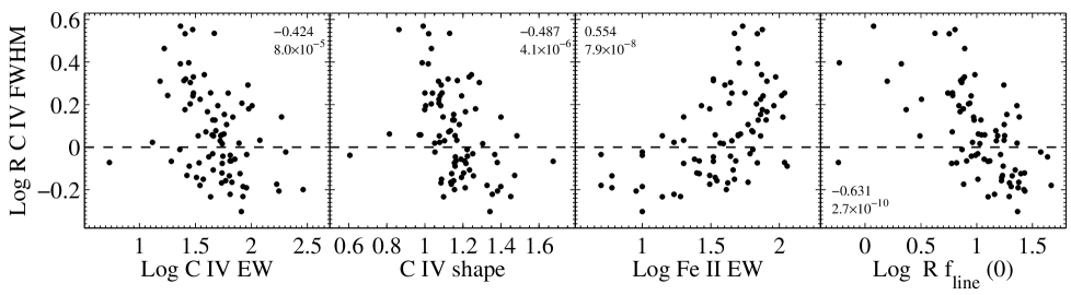
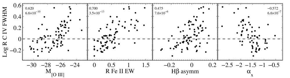
3.5 The R C iv FWHM

Figure 5 presents most of the significant correlations between R C iv FWHM and the various other parameters. The strongest correlations are with parameters related to the Fe II strength, the [O iii] strength, and the H$\rm\beta$ asymmetry. These parameters are part of the BG92 set of correlated optical emission line properties, which they termed eigenvector 1 (EV1). Narrow Line Seyfert 1 galaxies, NLS1s, generally populate the extreme end of EV1 (Osterbrock & Pogge 1985, and citations thereafter), with strong Fe II emission, weak [O iii] emission, and blue excess H$\rm\beta$ asymmetry. As shown in Fig. 5, in such objects the C iv line is broader than H$\rm\beta$. Large R C iv FWHM objects also have a steep $\alpha_{\rm x}$, consistent with the strong correlation between $\alpha_{\rm x}$ and EV1 (Laor et al. 1997b), and they also show weaker C iv emission, consistent with the known tendency of NLS1s to show weaker C iv emission (Wills et al. 1999; Shang et al. 2003). A new result shown in Fig. 5 is that the weakness of C iv relative to H$\rm\beta$ is more pronounced when looking at the relative line flux densities at $v=0$ km s^-1. This probably results from the combined effect of the broadening and weakening of the C iv emission in NLS1s. In addition, we find here that large R C iv FWHM objects tend to have line shape parameters closer to unity.

Figure 5: The dependence of the C iv to H$\rm\beta$ FWHM ratio on various parameters. The values of $r_{\rm S}$ and Pr are indicated in each panel. Objects where C iv is significantly broader than H$\rm\beta$ (above the dashed line) tend to have weak C iv, strong Fe ii, weak [O iii], steep $\alpha_{\rm X}$, and blue asymmetric H$\rm\beta$, parameters which are all related to the BG92 EV1.

Table 3: Conversion of $r_{\rm S}$${}^{\ref{fn:3a}}$ to Pr${}^{\ref{fn:3b}}$, as a function of $N$${}^{\ref{fn:3c}}$.

$|$$r_{\rm S}$$|$	$N=$
	81	75	69	65	54
0.1	$-0.427$	$-0.405$	$-0.383$	$-0.369$	$-0.326$
0.2	$-1.134$	$-1.069$	$-1.003$	$-0.958$	$-0.833$
0.3	$-2.187$	$-2.049$	$-1.911$	$-1.819$	$-1.560$
0.4	$-3.666$	$-3.423$	$-3.18$	$-3.017$	$-2.564$
0.45	$-4.602$	$-4.292$	$-3.98$	$-3.771$	$-3.194$
0.5	$-5.697$	$-5.306$	$-4.914$	$-4.652$	$-3.927$
0.55	$-6.98$	$-6.495$	$-6.008$	$-5.682$	$-4.783$
0.6	$-8.491$	$-7.894$	$-7.294$	$-6.894$	$-5.789$
0.65	$-10.287$	$-9.555$	$-8.822$	$-8.332$	$-6.981$
0.7	$-12.45$	$-11.556$	$-10.661$	$-10.063$	$-8.414$
0.8	$-18.48$	$-17.132$	$-15.783$	$-14.883$	$-12.402$
0.9	$-29.493$	$-27.312$	$-25.13$	$-23.675$	$-19.667$

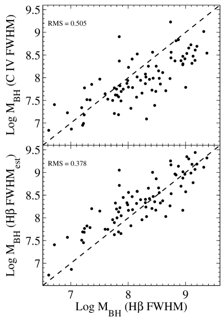
We note in passing that the correlations of the C iv EW, C iv luminosity and C iv shape with R C iv FWHM can be applied for improving the accuracy of the C iv based $M_{\rm BH}$ estimates. Specifically, the measured values of C iv EW, shape and luminosity, can be used to calculate the likely value of R C iv FWHM, e.g. based on a linear regression fit, and that value can then be used to infer the likely value of H$\rm\beta$ FWHM for a given C iv FWHM. This estimated H$\rm\beta$ FWHM can then be used to calculate $M_{\rm BH}$, thus overcoming part of the large scatter present in C iv based $M_{\rm BH}$ estimates. A search for the tightest correlation between $\log$ H$\rm\beta$ FWHM and a linear combination of $\log$ C iv FWHM, $\log$(C iv EW), $\log L$(C iv) and C iv shape yields a best fit relation

$$\begin{array}[]{l}\log({\rm H\beta~{}FWHM_{est}})=\log({\rm\mbox{C\,{\sc iv}}~{}FWHM})\\ +0.25\log({\rm\mbox{C\,{\sc iv}}~{}EW})+0.13\log[L({\rm\mbox{C\,{\sc iv}}})]\\ +0.4({\rm\mbox{C\,{\sc iv}}~{}shape})-6.6,\end{array}$$ (1)

where the EW is in units of Å, and $L({\rm\mbox{C\,{\sc iv}}})$ is in units of erg s^-1. Figure 6, upper panel, shows the $M_{\rm BH}$ estimates based on C iv (following Vestergaard 2002) versus the estimate based on H$\rm\beta$, which shows a dispersion of 0.505 (log scale), while the lower panel shows instead a comparison with $M_{\rm BH}$ derived using ${\rm H\beta~{}FWHM_{est}}$ rather than C iv FWHM. The dispersion reduces to 0.378, which is smaller, but still considerable. Thus, in the absence of direct observations of H$\rm\beta$, the UV based ${\rm H\beta~{}FWHM_{est}}$ may provide a somewhat more accurate estimate of $M_{\rm BH}$ than provided by the C iv FWHM.

Figure 6: Upper panel: the $M_{\rm BH}$ estimates based on C iv (following Vestergaard 2002) versus the estimate based on H$\rm\beta$. Note the large dispersion (0.505 in log scale) measured around a 1:1 relation (noted by the dashed line). Lower panel: as above, using the ${\rm H\beta~{}FWHM_{est}}$ rather than the C iv FWHM. Note the reduced but still significant dispersion (0.378). Thus, in the absence of direct observations of H$\rm\beta$, the UV based ${\rm H\beta~{}FWHM_{est}}$ may provide a somewhat more accurate estimate of $M_{\rm BH}$ than provided by the C iv FWHM.

The EV1 correlations are commonly interpreted as physical changes in the AGN properties which are related to the value of $L/L_{\rm Edd}$ (e.g. BG92). Figure 7 shows there is indeed a strong correlation of R C iv FWHM with $L/L_{\rm Edd}$ ($r_{\rm S}$ = 0.604). A plausible physical explanation for this effect is an outflowing wind component in the BLR, driven by a large $L/L_{\rm Edd}$, which can produce a higher column density outflow and thus a higher line emissivity. Such an outflow will have a lower density (due to expansion and increased speed), and would contribute mostly to the higher ionization lines, producing a broadened, shifted, and blue asymmetric C iv line (Section 1). The lower ionization lines, such as H$\rm\beta$, may originate from denser lower ionization gas, lying deeper within the BLR structure, which would be less affected by radiation pressure, and mostly dominated by gravity. However, Fig. 7 shows there is an even stronger correlation of R C iv FWHM with $M_{\rm BH}$ ($r_{\rm S}$ = $-$0.770), for which we find no clear physical explanation. Both correlations shown in Fig. 7 could however be induced by the tight relation between R C iv FWHM and H$\rm\beta$ FWHM ($r_{\rm S}$ $=-0.814$; Table 2), and the fact that $L/L_{\rm Edd}$ and $M_{\rm BH}$ are correlated with the H$\rm\beta$ FWHM. The partial correlations of R C iv FWHM with $L/L_{\rm Edd}$ and $M_{\rm BH}$, for a fixed H$\rm\beta$ FWHM, are indeed insignificant in our sample ($r_{\rm S}$ of $-0.099$ and $-0.183$, respectively). This does not preclude the above scenario of a physical relation between R C iv FWHM and $L/L_{\rm Edd}$, but in order to test it one needs a sample of AGN covering a wide range of $L/L_{\rm Edd}$ at a fixed H$\rm\beta$ FWHM. This will allow one to separate out the dependence of R C iv FWHM on $L/L_{\rm Edd}$ (or $M_{\rm BH}$) from its dependence on H$\rm\beta$ FWHM. To achieve that, one needs a sample of AGN covering a wide range in luminosity (e.g. Yuan & Wills 2003, figs. 4 & 5 there).

Figure 7: Left panel: the relation between R C iv FWHM and $L/L_{\rm Edd}$. A high R C iv FWHM occurs only at a high $L/L_{\rm Edd}$, but there are high $L/L_{\rm Edd}$ objects where R C iv FWHM is low (the profiles of the circled objects appear in Fig. 8). Right panel: the relation between R C iv FWHM and $M_{\rm BH}$. The values of $r_{\rm S}$ and Pr are indicated in two rows for each plot. The upper row is for the plotted correlation, and the lower row for the partial correlation at a fixed H$\rm\beta$ FWHM. Both partial correlations are insignificant, indicating the apparently strong correlations plotted here may be induced by the correlation of the H$\rm\beta$ FWHM with $L/L_{\rm Edd}$, and $M_{\rm BH}$.

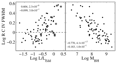
Despite the plausibility of the high $L/L_{\rm Edd}$ driven BLR outflow scenario, Fig. 7 clearly demonstrates that although a high $L/L_{\rm Edd}$ is necessary for a large R C iv FWHM (there are no large R C iv FWHM objects at low $L/L_{\rm Edd}$), it is clearly not sufficient (there are low R C iv FWHM objects at a high $L/L_{\rm Edd}$). This is further demonstrated in Figure 8 which shows two different types of line profiles in objects with a high $L/L_{\rm Edd}$ ($\ga 0.8$). The left panel shows the C iv and H$\rm\beta$ profiles of I Zw 1 and three more ‘I Zw 1-like’ objects in our sample. All objects have a large values of R C iv FWHM, a large C iv blue-shift, and a large blue excess asymmetry (see Leighly & Moore 2004 for two additional examples). Such objects are found only at high $L/L_{\rm Edd}$ values (Fig. 7), which supports the $L/L_{\rm Edd}$ driven outflow interpretation. However, the right panel in Fig. 8 shows the profiles of four other high $L/L_{\rm Edd}$ objects where R C iv FWHM is small ($\la 0$), the C iv line shift is small, and the line profiles are symmetric. Thus, having a high $L/L_{\rm Edd}$ appears to be a necessary, but not sufficient, condition for having ‘I Zw 1-like’ C iv profiles. What is the difference between the ‘normal’ and ‘I Zw 1-like’ objects at a high $L/L_{\rm Edd}$? A correlation analysis of the various emission parameters with R C iv FWHM for the subset of $L/L_{\rm Edd}$ $>0.5$ objects did not yield new correlations beyond those present for the complete sample. We note, anecdotally, that all the objects on the left panel of Fig. 8 have relatively weak soft X-ray emission (PG 1259+593, PG 1543+489, Brandt et al. 2000), or show significant X-ray and UV absorption (PG 0050+124, Gallo et al. 2004, Purquet et al. 2004; PG 2112+059, Gallagher et al. 2004a), while none of the objects on the right panel show evidence for either effects. This trend is consistent with the result of Gallagher et al. (2004b) that AGN with a blueshifted C iv emission show excess X-ray absorption compared to normal AGN. A possible interpretation of the above trend is that the outflow component indicated by the ‘I Zw 1-like’ C iv profile also tends to absorb the UV and/or X-ray emission. However, it does not explain why radiation pressure does not produce such an outflow in a significant fraction of high $L/L_{\rm Edd}$ AGN.

Figure 8: Not all high $L/L_{\rm Edd}$ ($\ga 0.8$) objects are alike. Left panel: four high $L/L_{\rm Edd}$ objects with ‘I Zw 1-like’ C iv profiles (upper left object is I Zw 1), i.e. where C iv is strongly blueshifted and with a blue asymmetric profile. A similar, but significantly weaker effect is seen in H$\rm\beta$. Right panel: four high $L/L_{\rm Edd}$ objects where the C iv and H$\rm\beta$ profiles are quite similar. The name of the object is indicated at the left side of each panel, and log $L/L_{\rm Edd}$ is indicated at the right side of each panel.

3.6 Other correlations

Below we discuss various other correlations found in our sample, and compare them to some correlations found in earlier studies.

3.6.1 C iv Shift versus EW

Espey et al. (1989) noted an inverse relation between the shift of the C iv line peak, measured with respect to H$\rm\alpha$, and the C iv EW, such that the line peak becomes more blueshifted as it becomes weaker. Similar correlations were found by Corbin (1990), where the C iv shift was measured with respect to Mg ii, and by Marziani et al. (1996; shift relative to H$\rm\beta$). Richards et al. (2002) constructed composite spectra for 794 SDSS quasars based on the C iv versus Mg ii velocity shift, and also found a decreasing C iv EW with increasing shift. Here we confirm the C iv EW versus shift correlation ($r_{\rm S}$ = 0.376, Table 2, note that the correlation sign is positive here since a shift to the blue is defined as negative), but we note that the C iv EW shows significantly stronger correlations with other parameters, in particular those related to the strength of Fe ii, [O iii] and $\alpha_{\rm ox}$. The C iv shift shows comparable strength correlations with parameters related to the strength of Fe ii and [O iii].

Richards et al. (2002) found that the C iv EW versus shift correlation appears to be induced by absorption of the red wing of C iv, rather than a true shift of the line, which they suggested (among other options) may imply that this correlation is induced by inclination dependent absorption effects, rather than physical changes in the BLR properties. However, the strong correlations of the C iv EW with some of the BG92 EV1 parameters mentioned above, and the various evidence that the EV1 correlations are driven by $L/L_{\rm Edd}$ (see also BL04) argue that the correlation of the C iv EW with the C iv shift is not just an inclination effect, but may rather be induced by the dependence of both parameters on $L/L_{\rm Edd}$.

3.6.2 Correlations with Fe ii EW

Marziani et al. (1996) find significant correlations of R Fe ii EW with R C iv EW and C iv shift, which we verify here (Table 2), although we find that R Fe ii EW shows stronger correlations with the C iv EW and with R FWHM. As mentioned in BL04, the inverse relation between the Fe ii and C iv strength may be an optical depth effect, where large resonance line optical depth results in the conversion of UV Fe ii to optical Fe ii (Netzer & Wills 1983; Shang et al. 2003), and the collisional destruction of the C iv line (Ferland et al. 1992). Alternatively, the Fe ii and C iv lines may originate in different populations of clouds in the BLR, and the inverse relation can be induced by the dominance of one population at the expense of the other, e.g. due to obscuration (T. Boroson, private communication).

In the ‘single population of clouds’ interpretation the differences between the C iv and H$\rm\beta$ line profiles may be induced by a velocity dependent optical depth in the BLR. For example, at higher velocities the line optical depth may drop, causing enhancement of C iv emission and suppression of the optical Fe ii. Alternatively, in the ‘two populations of clouds’ interpretation the difference in profiles may result from different physical locations of the two populations. For example, higher ionization lines may originate closer to the center, making C iv broader than H$\rm\beta$. However, both interpretations do not explain naturally why C iv becomes narrower than H$\rm\beta$ when the H$\rm\beta$ FWHM $>4000~{}$km s^-1. A possible alternative interpretation for the inverse trend in line widths is that H$\rm\beta$ and C iv have orthogonal velocity fields. For example, H$\rm\beta$ originating in a high density low ionization Keplerian disk component, and C iv in a lower density higher ionization radial outflow component (e.g. Wills et al. 1993a). The H$\rm\beta$ FWHM $<4000$ km s^-1 objects would then represent ‘face on BLR disk’ objects and H$\rm\beta$ FWHM $>4000$ km s^-1 ‘edge on’ objects (e.g. Wills & Browne 1986). If true, that would imply that the H$\rm\beta$ based $M_{\rm BH}$ estimates could be biased, but there is no current supporting evidence for such a bias. Velocity resolved reverberation mapping will be invaluable in disentangling the spatial distribution of the low and high ionization line emission as a function of velocity in the BLR (e.g. Horne et al. 2004).

3.7 Notable noncorrelations

The correlation strength between the C iv and H$\rm\beta$ shift, shape, and asymmetry parameters are, respectively, 0.173, $-0.173$, and 0.136, which are all insignificant (see Table 3). This lack of correlation is surprising. For example, if the H$\rm\beta$ and C iv blue excess asymmetry were produced by radiation pressure effects, which may produce a large asymmetry in C iv and a weaker one in H$\rm\beta$, then one would expect the amount of line asymmetry to be correlated as both would be driven by $L/L_{\rm Edd}$. The lack of significant correlations between the C iv and H$\rm\beta$ profile parameters suggests that unrelated mechanisms influence the two line profiles.

The C iv shift and shape parameters show at most marginally significant correlations with the various optical and UV emission parameters explored here. The C iv asymmetry shows no significant correlations at all (and was therefore not included in Table 2). This, again, argues against the idea that the C iv asymmetry is generally induced by radiation pressure effects, which should have produced a correlation with $L/L_{\rm Edd}$ and some of the EV1 parameters. Corbin & Boroson (1996) found a significant correlation ($-0.650$) between the C iv asymmetry and the luminosity at 1549 Å, however we find no significant correlation here ($r_{\rm S}$ $=-0.078$). Also, Sulentic et al. (2000) suggest there is a significant correlation between the C iv shift/C iv EW ratio and the H$\rm\beta$ FWHM, again this correlation is not significant in our sample.

Leighly & Moore (2004) find a significant correlation between the C iv asymmetry and C iv EW in a sample of NLS1s. Here we find in our corresponding sub-sample of 17 narrow line PG AGN with H$\rm\beta$ FWHM $<2000$ km s^-1, a correlation of 0.314 (but only 0.007 for the complete sample) which is not significant. Leighly (2004b) finds a significant correlation between the fraction of the C iv line flux at $v<$ 0 km s^-1 and C iv EW and $\alpha_{\rm ox}$ in their NLS1s sample. Here we find in our corresponding sample correlations of $-$0.483 for the C iv EW versus the C iv line flux at $v<$ 0 km s^-1, which is marginally significant, and $-$0.053 for the correlation with $\alpha_{\rm ox}$, which is clearly insignificant.

3.8 Indicators for dust absorption and scattering

AGN display a range of optical-UV spectral slopes. This range could be an intrinsic property of the continuum production mechanism, or it may, at least in part, be induced by intrinsic dust extinction. Below we present a set of correlations of various parameters with $\alpha_{\rm o,UV}$, which suggest that dust has noticeable effects on the continuum and line emission in our AGN sample, despite its relatively blue color selection criterion.

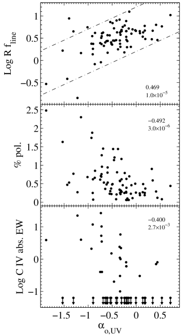
Figure 9, upper panel, shows there is a significant correlation between the C iv/H$\rm\beta$ flux ratio and $\alpha_{\rm o,UV}$, such that AGN with a redder continuum tend to have a relatively weaker C iv emission. A similar trend of weaker C iv emission in redder quasars was noted by Richards et al. (2003). The two diagonal lines in the upper panel, which bound the distribution of most of the objects, represent the effects of absorption by a foreground screen which suppresses both the line and continuum emission by the same factor. This correlation appears to indicate that some of the range in the C iv/H$\rm\beta$ flux ratio is due to absorption by dust outside the BLR (as expected due to sublimation, Laor & Draine 1993), which reddens both the lines and the continuum at a given wavelength by the same amount. The intrinsic range in the C iv/H$\rm\beta$ flux ratio may thus be closer to a factor of $\sim 10$, rather than $\sim 30$ as Fig. 9 indicates. The C iv/H$\rm\beta$ flux ratio also shows a strong correlation with $\alpha_{\rm ox}$ (Table 2). Since the dust X-ray (2 keV) absorption is negligible compared to the optical one (e.g. fig. 6 in Laor & Draine 1993), it cannot explain the correlation with $\alpha_{\rm ox}$, which may reflect the dependence of the intrinsic C iv/H$\rm\beta$ line ratio on the shape of the ionizing continuum (e.g. Korista et al. 1998). Interestingly, the same trends were already noted by Netzer et al. (1995) for the Ly$\alpha$/H$\rm\beta$ line ratio, which they find is also strongly correlated with both $\alpha_{\rm o,UV}$ and $\alpha_{\rm ox}$, and which they interpret as above.

The second panel shows there is a significant correlation of the visible (white) light percentage polarization (Berriman et al. 1990) and $\alpha_{\rm o,UV}$, such that the highest polarization increases as the objects become redder. A plausible interpretation is that redder objects tend to have a larger covering factor of dust, which will scatter a larger fraction of the continuum light and produce a stronger component of polarized scattered light. The increased extinction of the transmitted, presumably unpolarized light, in steep $\alpha_{\rm o,UV}$ objects also increases the relative contribution of the polarized light, and thus the percentage polarization. The presence of low polarization objects at the steepest $\alpha_{\rm o,UV}$ may be produced by geometrical dilution of the polarization amplitude, as the polarization tends to zero towards a face-on view of an azimuthally symmetric scattering source. Strongly reddened and polarized continua are commonly observed in far IR selected AGN (e.g. Wills 1999; Antonucci 2002; Hines et al. 2001), and the above correlation suggests it extends with a smaller amplitude to blue color selected AGN, such as the PG quasar sample.

The third panel shows there is a significant correlation between $\alpha_{\rm o,UV}$ and the C iv absorption EW (from Laor & Brandt 2002), such that redder objects tend to have stronger C iv absorption. This result is consistent with the finding of Constantin & Shields (2003) that NLS1s with UV absorption lines are on average redder than those without absorption, and the finding of Hopkins et al. (2004) that intrinsic narrow UV absorption lines are more common in redder quasars. An association between UV absorption and reddening was established by Sprayberry & Foltz (1992) for low ionization broad absorption line quasars (BALQs), and was later shown by Brotherton et al. (2001) to extend with a smaller amplitude to all BALQs. Our results suggest the UV absorption - reddening association is present already at a UV absorption EW level of $\sim$ 1-10 Å.

A plausible interpretation for this correlation is that the C iv absorption arises in gas associated with the dust which produces the reddening (e.g. Crenshaw & Kraemer 2001). Alternatively, the dust and C iv absorbers may be spatially distinct but coplanar. For example, the dust absorption may originate in a torus like structure, while the C iv absorption may arise from an equatorial wind launched from an accretion disk which is coplanar with a larger scale torus. We note in passing that the C iv absorption is also correlated with $\alpha_{\rm ox}$ (Brandt et al. 2000), which may indicate the presence of an X-ray absorbing component coplanar with the C iv absorber. Since the C iv emission strength is also correlated with $\alpha_{\rm ox}$, the X-ray absorber is likely to exist inside the BLR, in order to affect the ionizing continuum incident on the BLR.

Evidence for an association between reddening, UV absorption, and a planar structure is seen in radio galaxies (Baker & Hunstead 1995; Barthel, Tytler & Vestergaard 1997; Baker et al. 2002; Vestergaard 2003). A similar picture appears to hold for broad absorption line quasars, which apart from the redder continuum mentioned above, also show a higher polarization (e.g. Schmidt & Hines 1999; Ogle et al. 1999), and a weaker C iv emission (Turnshek 1984; Hartig & Baldwin 1986). The correlations shown in Fig.9 suggest that this picture may also extend to optically blue selected quasars.

Figure 9: Indications for dust absorption and scattering. Upper panel: the relation of the C iv/H$\rm\beta$ flux ratio and $\alpha_{\rm o,UV}$. The dashed lines indicate the effects of absorption of the lines and the continuum by the same amount at a given wavelength. The reddening of the continuum and weakening of C iv may be induced by a foreground dust screen. Middle panel: the relation of the white light polarization and $\alpha_{\rm o,UV}$. This may be induced by a contribution of dust scattered and polarized light, which increases in relative strength with increasing dust covering factor and optical depth. Lower panel: the relation of the C iv absorption EW (measured for 54 objects) and $\alpha_{\rm o,UV}$. The C iv absorption and continuum reddening may arise in a foreground dusty gas, or it could arise in coplanar but spatially distinct components.

4 Conclusions

A study of the C iv and H$\rm\beta$ emission line profiles in a nearly complete sample of 81 low $z$ optically selected quasars reveals the following:

1. Narrow C iv lines (FWHM $<2000$ km s^-1) are rare ($\sim 2$ per cent occurrence rate) compared to narrow H$\rm\beta$ ($\sim 20$ per cent).

2. When the H$\rm\beta$ FWHM $<4000$ km s^-1 the C iv line is broader than H$\rm\beta$, but the reverse is true when the H$\rm\beta$ FWHM $>4000$ km s^-1. This argues against the view that C iv generally originates further inward in the BLR compared with H$\rm\beta$.

3. C iv appears to provide a significantly less accurate, and possibly biased estimate of the black hole mass in AGN, compared with H$\rm\beta$.

4. The line profile differences are correlated with some of the BG92 eigenvector 1 parameters, which may be related to the relative accretion rate $L/L_{\rm Edd}$. A high $L/L_{\rm Edd}$ appears to be a necessary, but somehow not sufficient condition for having strongly blueshifted and asymmetric C iv emission.

Thus, a simple understanding of what controls the C iv profile and the large range in C iv to H$\rm\beta$ FWHM ratio remains a challenge.

5. There are indications for dust reddening and scattering in ‘normal’ optically selected AGN. In particular, PG quasars with a redder optical-UV continuum slope show weaker C iv emission, stronger C iv absorption, and a higher continuum polarization.

Reverberation mappings of AGN with highly discrepant H$\rm\beta$ and C iv profiles can provide important constraints on the spatial distribution of the line emissivity as a function of velocity, and thus test the various scenarios for the origin of the large profile differences.

References

- Antonucci (2002) Antonucci R., 2002, Astrophysical Spectropolarimetry, 151
- Baker & Hunstead (1995) Baker J. C., Hunstead R. W., 1995, ApJ, 452, L95
- Baker et al. (2002) Baker J. C., Hunstead R. W., Athreya R. M., Barthel P. D., de Silva E., Lehnert M. D., Saunders R. D. E., 2002, ApJ, 568, 592
- Baldwin & Netzer (1978) Baldwin J. A., Netzer H., 1978, ApJ, 226, 1
- Baldwin et al. (1996) Baldwin J. A. et al., 1996, ApJ, 461, 664
- Barthel (1997) Barthel P. D., Tytler D., Vestergaard M., 1997, in ASP Conf. Ser. 128, Mass Ejection from AGN, ed. N. Arav, I. Shlosman, R. J. Weymann (San Francisco: ASP), 48
- Baskin & Laor (2004) Baskin A., Laor A., 2004, MNRAS, 350, L31 (BL04)
- Berriman et al. (1990) Berriman G., Schmidt G. D., West S. C., Stockman H. S., 1990, ApJS, 74, 869
- Boroson & Green (1992) Boroson A. T., Green R. F., 1992, ApJS, 80, 109 (BG92)
- Brandt, Laor, & Wills (2000) Brandt W. N., Laor A., Wills B. J., 2000, ApJ, 528, 637
- Brotherton et al. (2001) Brotherton M. S., Tran H. D., Becker R. H., Gregg M. D., Laurent-Muehleisen S. A., White R. L., 2001, ApJ, 546, 775
- Collin-Souffrin, Dumont, & Tully (1982) Collin-Souffrin S., Dumont S., Tully J., 1982, A&A, 106, 362
- Constantin & Shields (2003) Constantin A., Shields J. C., 2003, PASP, 115, 592
- Corbett et al. (2003) Corbett E. A., et al., 2003, MNRAS, 343, 705
- Corbin (1991) Corbin M. R., 1991, ApJ, 371, L51
- Corbin & Boroson (1996) Corbin M. R., Boroson T. A., 1996, ApJS, 107, 69
- Crenshaw & Kraemer (2001) Crenshaw D. M., Kraemer S. B., 2001, ApJ, 562, L29
- De Robertis (1985) De Robertis M., 1985, ApJ, 289, 67
- Dietrich & Hamann (2004) Dietrich M., Hamann F. 2004, ApJ, in press
- Espey et al. (1989) Espey B. R., Carswell R. F., Bailey J. A., Smith M. G., Ward M. J., 1989, ApJ, 342, 666
- Ferland et al. (1992) Ferland G. J., Peterson B. M., Horne K., Welsh W. F., Nahar S. N., 1992, ApJ, 387, 95
- Ferrarese et al. (2001) Ferrarese L., Pogge R. W., Peterson B. M., Merritt D., Wandel A., Joseph C. L., 2001, ApJ, 555, L79
- Gallagher et al. (2004) Gallagher S. C., Brandt W. N., Wills B. J., Charlton J. C., Chartas G., Laor A., 2004a, ApJ, 603, 425
- Gallagher et al. (2004) Gallagher S. C., Richards G. T., Hall P. B., Brandt W. N., Schneider D. P., Vanden Berk D. E., 2004b, AJ, submitted
- Gallo et al. (2004) Gallo L. C., Boller T., Brandt W. N., Fabian A. C., Vaughan S., 2004, A&A, 417, 29
- Gaskell (1982) Gaskell C. M., 1982, ApJ, 263, 79
- Gebhardt et al. (2000) Gebhardt K., et al., 2000, ApJ, 543, L5
- Halpern, Eracleous, Filippenko, & Chen (1996) Halpern J. P., Eracleous M., Filippenko A. V., Chen K., 1996, ApJ, 464, 704
- Hartig & Baldwin (1986) Hartig G. F., Baldwin J. A., 1986, ApJ, 302, 64
- Hines et al. (2001) Hines D. C., Schmidt G. D., Gordon K. D., Smith P. S., Wills B. J., Allen R. G., Sitko M. L., 2001, ApJ, 563, 512
- Hopkins (2004) Hopkins P. F., et al. 2004, AJ, in press (astro-ph/0406293)
- Horne, Peterson, Collier, & Netzer (2004) Horne K., Peterson B. M., Collier S. J., Netzer H., 2004, PASP, 116, 465
- Kaspi et al. (2000) Kaspi S., Smith P. S., Netzer H., Maoz D., Jannuzi B. T., Giveon U., 2000, ApJ, 533, 631
- Korista, Baldwin, & Ferland (1998) Korista K., Baldwin J., Ferland, G., 1998, ApJ, 507, 24
- Korista et al. (1995) Korista K. T. et al., 1995, ApJS, 97, 285
- Laor (1998) Laor A., 1998, ApJ, 505, L83
- Laor & Brandt (2002) Laor A., Brandt W. N., 2002, ApJ, 569, 641
- Laor & Draine (1993) Laor A., Draine B. T., 1993, ApJ, 402, 441
- Laor et al. (1994) Laor A., Banhcall J. N., Jannuzi B. T., Schneider D. P., Green R. F., Hatrig G. F., 1994, ApJ, 420, 110
- Laor, Jannuzi, Green, & Boroson (1997a) Laor A., Jannuzi B. T., Green R. F., Boroson T. A., 1997a, ApJ, 489, 656
- Laor et al. (1997b) Laor A., Fiore F., Elvis M., Wilkes B. J., McDowell J. C., 1997b, ApJ, 477, 93
- Leighly (2004a) Leighly K. M., 2004a, ApJ, in press (astro-ph/0402452)
- Leighly (2004b) Leighly K. M., 2004b, in Stellar-mass, Intermediate-mass, and Supermassive Black Holes, astro-ph/0402676
- Leighly & Moore (2004) Leighly K. M., Moore J. R., 2004, ApJ, in press (astro-ph/0402453)
- Marziani et al. (1996) Marziani P., Sulentic J. W., Dultzin-Hacyan D., Calvani M., Moles M., 1996, ApJS, 104, 37
- McIntosh, Rix, Rieke, & Foltz (1999) McIntosh D. H., Rix H.-W., Rieke M. J., Foltz C. B., 1999, ApJ, 517, L73
- Netzer (2003) Netzer H., 2003, ApJ, 583, L5
- Netzer & Wills (1983) Netzer H., Wills B. J., 1983, ApJ, 275, 445
- Netzer et al. (1995) Netzer H., Brotherton M. S., Wills B. J., Han M., Wills D., Baldwin J. A., Ferland G. J., Browne I. W. A., 1995, ApJ, 448, 27
- Neugebauer et al. (1987) Neugebauer G., Green R. F., Matthews K., Schmidt M., Soifer B. T., Bennett J., 1987, ApJS, 63, 615
- Ogle et al. (1999) Ogle P. M., Cohen M. H., Miller J. S., Tran H. D., Goodrich R. W., Martel A. R., 1999, ApJS, 125, 1
- Onken & Peterson (2002) Onken C. A., Peterson B. M., 2002, ApJ, 572, 746
- Osterbrock & Pogge (1985) Osterbrock D. E., Pogge R. W., 1985, ApJ, 297, 166
- Peterson et al. (2000) Peterson B. M. et al., 2000, ApJ, 542, 161
- Porquest et al. (2004) Porquet D., Reeves J. A., O’Brien P., Brinkmann W., 2004, A&A, in press (astro-ph/0404385)
- Richards et al. (2002) Richards G. T., Vanden Berk D. E., Reichard T. A., Hall P. B., Schneider D. P., SubbaRao M., Thakar A. R., York D. G., 2002, AJ, 124, 1
- Richards et al. (2003) Richards, G. T., et al., 2003, AJ, 126, 1131
- Schlegel, Finkbeiner, & Davis (1998) Schlegel D. J., Finkbeiner D. P., Davis M., 1998, ApJ, 500, 525
- Schmidt & Hines (1999) Schmidt G. D., Hines D. C., 1999, ApJ, 512, 125
- Schmidt & Green (1983) Schmidt M., Green R. F., 1983, ApJ, 269, 352
- Shemmer et al. (2004) Shemmer O., Netzer H., Maiolino R., Oliva E., Croom S., Corbett E., Di Fabrizio L., 2004, ApJ, in press
- Seaton (1979) Seaton M. J., 1979, MNRAS, 187, 73P
- Shang et al. (2003) Shang Z., Wills B. J., Robinson E. L., Wills D., Laor A., Xie B., Yuan J., 2003, ApJ, 586, 52
- Snedden & Gaskell (2004) Snedden S. A., Gaskell C. M., 2004, American Astronomical Society Meeting, 204, 4404
- Sprayberry & Foltz (1992) Sprayberry D., Foltz C. B., 1992, ApJ, 390, 39
- Steidel & Sargent (1991) Steidel C. C., Sargent W. L. W., 1991, ApJ, 382, 433
- Sulentic et al. (1995) Sulentic J. W., Marziani P., Dultzin-Hacyan D., Calvani M., Moles M., 1995, ApJ, 445, L85
- Sulentic, Marziani, & Dultzin-Hacyan (2000) Sulentic J. W., Marziani P., Dultzin-Hacyan D., 2000, ARA&A, 38, 521
- Sulentic, Zwitter, Marziani, & Dultzin-Hacyan (2000) Sulentic J. W., Zwitter T., Marziani P., Dultzin-Hacyan D., 2000, ApJ, 536, L5
- Turnshek (1984) Turnshek D. A., 1984, ApJ, 280, 51
- Tytler & Fan (1992) Tytler D., Fan X., 1992, ApJS, 79, 1
- Vanden Berk et al. (2001) Vanden Berk D. E. et al., 2001, AJ, 122, 549
- Vestergaard (2002) Vestergaard M., 2002, ApJ, 571, 733
- Vestergaard (2003) Vestergaard M., 2003, ApJ, 599, 116
- Vestergaard (2004) Vestergaard M., 2004, ApJ, 601, 676
- Wang, Brinkmann, & Bergeron (1996) Wang T., Brinkmann W., Bergeron J., 1996, A&A, 309, 81
- Warner, Hamann & Dietrich (2003) Warner C., Hamann F., Dietrich M., 2003, ApJ, 596, 72
- Warner, Hamann & Dietrich (2004) Warner C., Hamann F., Dietrich M., 2004, ApJ, 608, 136
- Wilkes (1984) Wilkes B. J., 1984, MNRAS, 207, 73
- Wilkes (1986) Wilkes B. J., 1986, MNRAS, 218, 331
- Wills & Browne (1986) Wills B. J., Browne I. W. A., 1986, ApJ, 302, 56
- Wills, Netzer, & Wills (1985) Wills B. J., Netzer H., Wills D., 1985, ApJ, 288, 94
- Wills et al. (1993a) Wills B. J., Brotherton M. S., Fang D., Steidel C. C., Sargent W. L. W., 1993a, ApJ, 415, 563
- Wills et al. (1993b) Wills B. J., Netzer H., Brotherton M. S., Han M., Wills D., Baldwin J. A., Ferland G. J., Browne I. W. A., 1993b, ApJ, 410, 534
- Wills et al. (1995) Wills B. J. et al., 1995, ApJ, 447, 139
- Wills et al. (1999) Wills B. J., Laor A., Brotherton M. S., Wills D., Wilkes B. J., Ferland G. J., Shang Z., 1999, ApJ, 515, L53
- Wills (1999) Wills B. J., 1999, ASP Conf. Ser. 162: Quasars and Cosmology, 101
- Yuan & Wills (2003) Yuan M. J., Wills B. J., 2003, ApJ, 593, L11