The CMB Spectrum in Cardassian Models

Abstract

The dark energy in the Universe is described in the context of modified Friedmann equations as a fluid parameterized by the density of dark matter and undergoing an adiabatic expansion. This formulation is applied to the Cardassian model. Choosing then parameters consistent with the supernova observations, it gives a background expansion in which the cosmic temperature fluctuations are calculated. The resulting spectrum is quite similar to what is obtained in the standard concordance model. If the Cardassian fluid is interpreted as a new kind of interacting dark matter, its overdensities are driven into oscillations when the interaction energy is rising in importance. This does not occur in a description of the Cardassian fluctuations motivated by theories of modified gravity. There the energy of the underlying matter is also conserved, which requires appearance of effective shear stress in the late Universe. In both approaches that allow fluctuations the thermal power spectrum at large scales is much too strongly enhanced by the late integrated Sachs-Wolfe effect. With the interacting dark matter assumption, we conclude that the Cardassian model is ruled out by observations, expect in a small neighbourhood of the $\Lambda$CDM limit.

Introduction

Observations of distant supernovae indicate that the expansion of the Universe now undergoes an accelerationRiess et al. (2004, 1998); Perlmutter et al. (1999). This is also consistent with the most recent and accurate measurements of the fluctuations in the cosmic microwave background by the WMAP satelliteSpergel et al. (2003). These also imply that the Universe is at least very nearly spatially flat.

A possible explanation of these observations requires that the Universe contains a new and unknown component, called dark energy, in addition to radiation, baryons and dark matter. This could be Einstein’s cosmological constant or a more dynamical component based on the universal presence of a scalar field called quintessenceZlatev et al. (1999); Caldwell et al. (1998). Alternatively, one could contemplate the possibility that standard Einstein gravity is not valid at very large scales so as to allow for modifications of the Friedmann equationsDvali et al. (2000); Carroll et al. (2004).

We will here consider one particular such proposal by Freese and LewisFreese and Lewis (2002) where the total energy density is made up of just the usual radiation, baryons and cold dark matter densities $\rho_{r}$, $\rho_{b}$ and $\rho_{c}$ but they enter in a non-linear way in the Friedmann equation for the scale parameter $a(t)$ in a spatially flat Universe,

$$H^{2}={8\pi G\over 3}g(\rho_{r},\rho_{b},\rho_{c})$$ (1)

where $H=\dot{a}/a$ is the Hubble parameter. There are several such proposals based on ideas from brane physicsChung and Freese (2000) or some unknown interactions between matter particlesGondolo and Freese (2003). But in order to make contact with the CMB physics, we will define the model so that the Friedmann equation takes the form

$$\left({\dot{a}\over a}\right)^{2}={1\over 3M^{2}}(\rho_{r}+\rho_{b}+\rho_{K})$$ (2)

where $M=(8\pi G)^{-\frac{1}{2}}$ is the reduced Planck mass and

$$\rho_{K}=\rho_{c}[1+B\rho_{c}^{-q\nu}]^{1/q}$$ (3)

is the modified polytropic Cardassian energy density. Here $B$ is a positive constant, $q$ is the polytropic index and it is modified as long as the parameter $\nu\neq 1$. All the unknown physics is now lumped into the dark sector. At early times when the matter density $\rho_{c}$ is large, the last term in (3) will be negligible and $\rho_{K}\approx\rho_{c}$. However, at late times when $\rho_{c}$ becomes small, the last term dominates and will act as a dark energy component due to unknown properties of dark matter. The energy fractions $\Omega_{i}=\rho_{i}/\rho_{cr}$ with $\rho_{cr}=3M^{2}H^{2}$, are seen from (2) to satisfy $\Omega_{r}+\Omega_{b}+\Omega_{K}=1$ since there is no curvature in space. In our calculations we use the WMAP valuesSpergel et al. (2003) for these parameters. Then $\Omega_{c}=0.226$, $\Omega_{b}=0.044$, and $\Omega_{r}$ we get from assuming three massless neutrino species and the background temperature $T=2.726~{}\mbox{K}$. For $h$ we use the value $0.72$. Today we will therefore have $\Omega_{K0}=1$ when we neglect the small contributions from radiation and baryons. Given $q$ and $\nu$, the remaining parameter $B$ follows then from

$$B=\rho_{cr}^{\,q\nu}\big{(}\Omega_{c0}^{-q}-1\big{)}\Omega_{c0}^{\,q\nu}.$$ (4)

Ordinary dark matter has zero pressure and satisfies the conservation equation $\dot{\rho}_{c}+3H\rho_{c}=0$ (in the homogeneous and isotropic background Universe). Thus we have $\rho_{c}=\rho_{c0}/a^{3}$, and correspondingly for the other standard ingredients, with $a=1$ today. The Friedmann equation (2) can then be integrated to give the full background evolution of the scale parameter $a(t)$ with Cardassian energy present.

Following Gondolo and FreeseGondolo and Freese (2003), we will assume that the Cardassian energy density $\rho_{K}$ is that of a fluid which undergoes an adiabatic expansion when the Universe evolves. It will thus have a pressure $p_{K}$ which can be obtained from its conservation equation $\dot{\rho}_{K}+3H(\rho_{K}+p_{K})=0$. Eliminating the Hubble parameter $H$ between this and the conservation equation for the dark matter, the Cardassian pressure will follow from

$$p_{K}=\rho_{c}{d\rho_{K}\over d\rho_{c}}-\rho_{K}.$$ (5)

For the choice (3) it gives

$$p_{K}=-\nu B\rho_{c}^{-q\nu+1}\Big{[}1+B\rho_{c}^{-q\nu}\Big{]}^{{1\over q}-1}.$$ (6)

This equation of state can be written on the standard form $p_{K}=w_{K}\rho_{K}$ with

$$w_{K}={-\nu B\rho_{c}^{-q\nu}\over 1+B\rho_{c}^{-q\nu}}.$$ (7)

At late times when $\rho_{c}\rightarrow 0$ we see that $w_{K}\rightarrow-\nu$. We therefore expect late-time acceleration when the parameter $\nu>1/3$. The equation-of-state parameter $w_{K}$ is zero at early times, and approaches the value $w_{K}=-\nu$ in the late universe, more rapidly for larger $q$. Late evolution of $w_{K}$ for different values of the parameters $q$ and $\nu$ is shown in Fig.1.

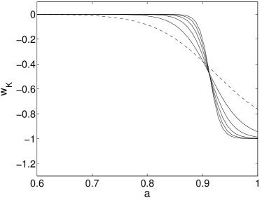
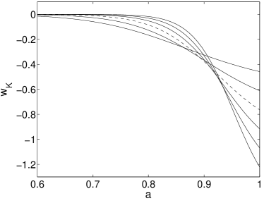
Figure 1: Equation-of-state parameter $w_{K}$ as a function of the scale factor. The upper panel has $\nu=1$ and $q$-values $q=1$,$2$,$3$,$4$,$5$ and $q=6$ (the steepest curve is for $q=6$). The lower panel has $q=1$ and $\nu=0.6$,$0.8$,$1.0$,$1.2$, $1.4$ and $\nu=1.6$ (the most negative $w_{K}$ today is for $\nu=1.6$). The dashed curves correspond to $\Lambda$CDM.

The late expansion history of these models has been compared to the observational data of supernovaeZhu and Fujimoto (2003); Wang et al. (2003) and of other astrophysical objectsZhu and Fujimoto (2002, 2004). The locations of acoustic peaks in the CMB spectrum has also been considered beforeSen and Sen (2003); Frith (2004). We will calculate the full CMB spectrum in these models, first assuming that the Cardassian component accounts only for the background expansion of the Universe. This would, however, correspond to a time-variable but nonfluctuating vacuum energy, to which we have no physical motivation. This is our case I.

A more realistic description, which allows fluctuations in the Cardassian fluid, is our case II. Then the Cardassian fluid can be thought of as an interacting dark matter. The energy density $\rho_{K}-\rho_{c}$ would then be attributed to an unknown particle species or field mediating the dark matter interactions. Thus $\rho_{c}$ does not satisfy an independent energy conservation law. It only satisfies a mass conservation law, whereas we have energy conservation for the total $\rho_{K}$.

In our case III we impose energy conservation separately for the cold dark matter. This can be motivated by theories of modified gravity. In these theories, we can generally write the Einstein equations as equations as

$$G_{\mu\nu}=\frac{1}{M^{2}}(T_{\mu\nu}^{M}+T_{\mu\nu}^{C}),$$ (8)

where $M$ is for matter and $C$ for the corrections to the standard gravity. The latter can be parameterized as a function of the matter energy density. We illustrate this with the example of corrections in the form of DGP gravityDvali et al. (2000),

$$H^{2}\pm\frac{H}{r_{0}}=\frac{1}{3M^{2}}\rho_{c}.$$ (9)

This can rewritten as

$$3M^{2}H^{2}=\rho_{c}+\frac{3M^{2}}{2r_{0}^{2}}\mp\left(\frac{9M^{4}}{4r_{0}^{4}}+\frac{3M^{2}}{r_{0}^{2}}\rho_{c}\right)^{\frac{1}{2}}.$$ (10)

The RHS we then interpret as an energy density of a fluid. Granted that the matter conservation also now applies as usually, we can find the pressure of this fluid

$$p = -2M^{2}[\frac{3}{2}\dot{H}+H^{2}]$$ (11)

$$= \mp\frac{\rho_{c}}{\left(1+\frac{4r_{0}^{2}}{3M^{2}}\rho_{c}\right)^{\frac{1}{2}}}-\frac{3M^{2}}{2r_{0}^{2}}\pm\left(\frac{9M^{4}}{4r_{0}^{4}}+\frac{3M^{2}}{r_{0}^{2}}\rho_{c}\right)^{\frac{1}{2}},nn$$ (12)

which gives the equation of state for this effective matter. It would also follow by using Eq.(5) with Eq.(10). However, in this paper we consider only Cardassian modifications to the Friedmann equation. For a recent investigation of the cosmological constraints for modifications generalized from Eq.(9), see Elgarøy and MultamäkiElgaroy and Multamaki (2004). Note also that we have included only the contribution from the density of dark matter in Eq.(9), because the corrections to the Einstein gravity do not become important until the matter dominated era. This justifies our use of Eq.(2) also in the case III.

Case I: No Cardassian fluctuations.

In order to calculate the temperature fluctuations in this Universe, we now consider these cases. Firstly we assume that the Cardassian fluid just provides a modified background for the evolution without any internal fluctuations. These take place in the ordinary components of radiation, baryons and dark matter and can be calculated by standard methods for any values of $q,\nu>0$. In Fig.2 we show the Bardeen potentials for the choice $\nu=0.8$ and $q=1.5$ and for different values of the wave number $k$ which sets the scale of the fluctuations. The evolution of gravitational potentials is seen to be very similar to what is found in $\Lambda$CDM models on all scales.

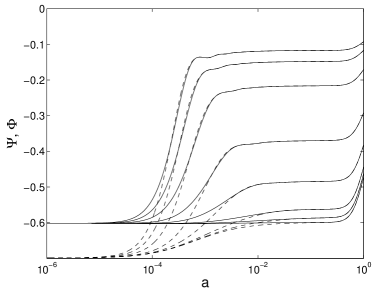
Figure 2: Evolution of $\Psi$ (solid line) and $\Phi$ (dashed line) in a Cardassian background (case I). From bottom to top, $k=0.00024,0.0012,0.0024,0.0060,0.012,0.036,0.048$ Mpc^-1.

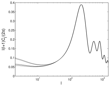
Figure 3: CMB spectra in a Cardassian background (case I). From bottom to up, $(q,\nu)=(1,1),(1.5,0.8),(2,0.7),(10,0.6)$ and $(100,0.6)$. The bottom curve with both $q$ and $\nu$ equal to 1 corresponds to the $\Lambda$CDM model.

We have calculated the CMB spectra using the fluid approximation for photons and the well known analytical result for the diffusion damping scale (e.g. Dodelson (2003)). We have tested the fluid approximation with various models and found it to be in agreement with more exact calculations (using e.g. CMBFASTSeljak and Zaldarriaga (1996)) within 5 per cent for $\ell$ smaller than a few hundred. This is sufficiently accurate to uncover the interesting large scale features of the models we are considering, as is the main purpose of this investigation. For simplicity, we do not include reionization. Our perturbations are normalized such that the primordial curvature perturbation $\mathcal{R}=1$.

In Fig.3 we show the full thermal spectrum obtained from this modified background. Here we use the same Cardassian parameters $(q,\nu)=(1,1),(1.5,0.8),(2,0.7),(10,0.6)$ and $(100,0.6)$ which have been found by Savage, Sugiyama and FreeseSavage et al. (2004) to be consistent with the SNIa observations and the age of the Universe. The peaks in the thermal spectra are located at the right places and the contribution from the integrated Sachs-Wolfe effect is seen to increase modestly with $q$. However, by lowering $q$ below $1$ one cannot reduce the ISW effect without losing the agreement of the spectrum with WMAP observations on smaller scales.

Case II: CDM fluctuations driven by the Cardassian fluid.

As our second approach, we include fluctuations in the Cardassian fluid. These will then drive the fluctuations in the underlying dark matter. In our discussion of perturbations we adopt the notation of Ma and BertschingerMa and Bertschinger (1995), with the only exception of using uppercase letters for the gravitational potentials in the conformal-Newtonian gauge. In this gauge the line element is then written as

$$ds^{2}=a^{2}(\tau)[-(1+2\Psi)d\tau^{2}+(1-2\Phi)\delta_{ij}dx^{i}dx^{j}].\quad$$ (13)

We assume adiabatic perturbations, which means that the relations (3) and (6) between $\rho_{K}$, $p_{K}$, and $\rho_{c}$ will hold also for the perturbed quantities.

Assuming no anisotropic stress in the Cardassian fluid, we find that its density perturbations in this gauge obey the equation of motion

$$\delta^{\prime}_{K}=(1+w_{K})(-\theta_{K}+3\Phi^{\prime})+3\mathcal{H}(w_{K}-c_{K}^{2})\delta_{K}$$ (14)

while the corresponding velocity perturbation is governed by

$$\theta_{K}^{\prime} = (3w_{K}-1){\cal H}\theta_{K}-w^{\prime}_{K}{\theta_{K}\over 1+w_{K}}$$ (15)

$$\mbox{}+{k^{2}c_{K}^{2}\delta_{K}\over 1+w_{K}}+k^{2}\Psi.$$

Here the prime denotes the derivative with respect to conformal time, ${\cal H}=a^{\prime}/a$ and the equation of state parameter $w_{K}$ is given by (7). Its conformal time derivative is then

$$w^{\prime}_{K}=-{3{\cal H}q\nu^{2}B\rho_{c}^{-q\nu}\over[1+B\rho_{c}^{-q\nu}]^{2}}$$ (16)

and goes to zero at late times. The remaining parameter is the Cardassian speed of sound $c_{K}^{2}\equiv(\partial p_{K}/\partial\rho_{K})_{s}=dp_{K}/d\rho_{K}$. From the pressure (6) we then find

$$c_{K}^{2}=\frac{\nu B\rho_{c}^{-q\nu}[(\nu-1)B\rho_{c}^{-q\nu}+q\nu-1]}{1+(2-\nu)B\rho_{c}^{q\nu}+(1-\nu)B^{2}\rho_{c}^{-2q\nu}}.$$ (17)

At late times when $\rho_{c}\rightarrow 0$ this is seen to approach $c_{K}^{2}\rightarrow-\nu$ which is unacceptable. This can be avoided only by choosing the special value $\nu=1$. Then the expression for the sound speed simplifies to

$$c_{K}^{2}={q-1\over 1+\rho_{c}^{q}/B}.$$ (18)

In order for it to be positive, we must have $q>1$ and also $q<2$ so that $c_{K}^{2}<1$ at late times.

We find it also useful to do the calculations in the synchronous gauge, in which the line element is given by

$$ds^{2}=a^{2}(\tau)[-d\tau^{2}+(\delta_{ij}+h_{ij})dx^{i}dx^{j}],$$ (19)

where we define the scalar modes in the Fourier space as

$$h_{ij}({\bf x},\tau) = \int d^{3}ke^{i{\bf k}\cdot{\bf x}}\biggl{[}\hat{k}_{i}\hat{k}_{j}h({\bf k},\tau)$$ (20)

$$\mbox{}+6(\hat{k}_{i}\hat{k}_{j}-\frac{1}{3}\delta_{ij})\eta({\bf k},\tau)\biggr{]},$$

when ${\bf k}=k\hat{k}$. In this gauge the fluctuation equations for a general fluid, which may have also anisotropic stress $\sigma$, are

$$\delta^{\prime}=-(1+w)(\theta+\frac{h^{\prime}}{2})+3\mathcal{H}(w-c^{2})\delta$$ (21)

for the density contrast and

$$\theta^{\prime}=(3w-1)\mathcal{H}\theta-\frac{w^{\prime}}{1+w}\theta+\frac{c^{2}}{1+w}k^{2}\delta-k^{2}\sigma$$ (22)

for the velocity perturbation.

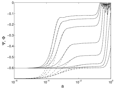
Figure 4: Evolution of $\Psi$ (solid line) and $\Phi$ (dotted line) in the presence of a Cardassian fluid (case II). From bottom to top, $k=0.00024,0.0012,0.0024,0.0060,0.012,0.036,0.048$ Mpc^-1.

We have numerically solved the perturbation equations in both gauges now including also the fluctuations in the Cardassian fluid for the representative value $q=1.5$. In this case the fluctuations in the dark matter are not independent. The evolution of the Bardeen potentials $\Psi$ and $\Phi$ at different scales is shown in Fig.4. They are seen to have a very rapid increase (decrease in absolute value) at late times for all scales comparable and smaller than the present horizon. This results in an unusually strong late-time ISW effect. In the thermal spectrum in Fig.5 it is seen to give a rather big deviation from the WMAP data for scales $\ell<100$. We find the same results in both gauges. The top curve is an example of a model where the sound speed of the Cardassian fluid exceeds the speed of light. Models where $c_{K}^{2}$ takes negative values are not computable at all since fluctuations then blow up, except for tiny deviations from the $\Lambda$CDM values.

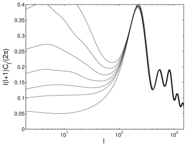
Figure 5: CMB spectra in the case II. Here $\nu=1$ and from bottom to up, $q=1,1.05,1.1,1.2,1.4,1.8$ and $2.6$.

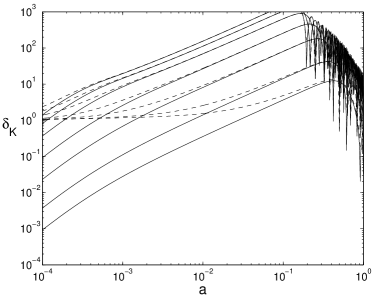
Figure 6: Evolution of $\delta_{K}$ in the case II. The model is the same as in Fig.4. From bottom to top, $k=0.0012,0.0024,0.0060,0.012,0.036,0.048$ Mpc^-1. Dashed lines represent the perturbations in Newtonian and the solid lines in the synchronous gauge.

The dynamics is now different from the case I, where the growth of matter perturbations was slowed down only because of the accelerated expansion of the background Universe. Now the overdensities, which have grown in the Cardassian fluid during its matter-like behaviour, are swiftly decaying as the fluid is turning into an effective cosmological constant. Meanwhile, the decaying overdensities perform rapid oscillations due to presence of the Cardassian pressure. This is shown in Fig.6. Fluctuations in the cold dark matter and in the Cardassian fluid are related adiabatically

$$\delta_{c}=\left(\frac{d\log\rho_{K}}{d\log\rho_{c}}\right)^{-1}\delta_{K}=\frac{\delta_{K}}{1+w_{K}}\sim a^{3q}\delta_{K},\quad$$ (23)

where the last equality holds at late times (and when $\nu=1$). From this we see that the dark matter perturbations are driven along with the Cardassian oscillations, but are not sharing the decay rate of the host fluid perturbations.

The Cardassian fluid which is restricted here to have the two parameters $\nu=1$ and $1<q<2$, is related to the generalized Chaplygin gas (GCG)Bento et al. (2002). In the latter model the energy density is

$$\rho_{GCG}=[B+\frac{A}{a^{3(1+\alpha)}}]^{\frac{1}{1+\alpha}}.$$ (24)

After the change of variable, $q=1+\alpha$, we see that this reduces to the Cardassian model in the special case that $\nu=1$ (A is fixed by requiring standard early cosmology). In the Cardassian model we consider cold dark matter existing separately and that its perturbations obey Eq.(23). But the resulting CMB spectrum should be equivalent regardless of this intrinsic decomposition of the fluid. Indeed, our results agree withAmendola et al. (2003), where the CMB spectrum was calculated for the generalized Chaplygin gas. Note that there the normalization of the spectra is different from ours, since there the Sachs-Wolfe plateau is kept low, resulting in lower amplitude at small scales.

For completeness, we consider also the matter power spectra in these models. We define here the total matter power spectrum, including both the contribution from the Cardassian fluid and from the baryons, as

$$P(k)=\frac{k^{3}}{2\pi^{2}}|\delta_{k}|^{2}=\frac{k^{3}}{2\pi^{2}}\left(\frac{\rho_{K}\delta_{K}+\rho_{b}\delta_{b}}{\rho_{K}+\rho_{b}}\right)^{2}.$$ (25)

In the Fig.7 we see that modifying only the background evolution has little effect on the matter power spectrum. However, as shown also by Amarzguioui, Elgarøy and MultamäkiAmarzguioui et al. (2004), consistently with Sandvik, Tegmark and ZaldarriagaSandvik et al. (2004), when one adopts the fluid interpretation of the Cardassian expansion, even tiny changes in the parameters $q$,$\nu$ result in observable departure from the $\Lambda$CDM cosmology in the matter power spectrum. This is seen in Fig.8. When $c_{S}^{2}<0$, the spectrum blows up. When $c_{S}^{2}>0$, the spectrum of Cardassian fluid would be oscillating as expected from Fig.6, but these are not seen in the total matter power spectrum since $\delta_{K}$ is suppressed and thus the baryonic fluctuations dominate the structure at smaller scales. Also the amplitude of the total matter power spectrum is sensitive to the parameters $q$ and $\nu$.

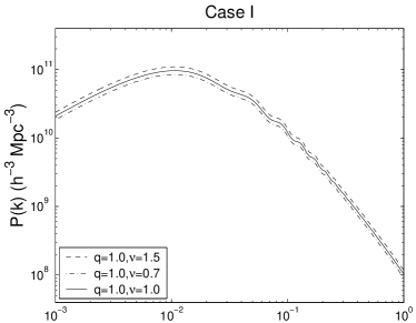
Figure 7: The total matter power spectra for different parameter values in case I.

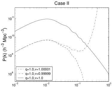
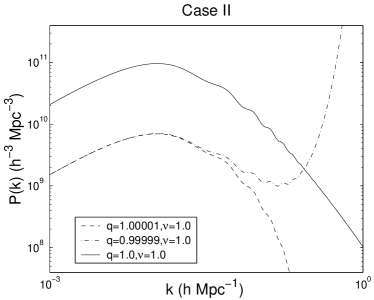
Figure 8: The total matter power spectra for different parameter values in case II.

There has been some interesting suggestions on how to render the growth of structure in the GCG model more plausibleReis et al. (2003); Bento et al. (2004). The one proposed inReis et al. (2003) imposes intrinsic entropy perturbations in the fluid to cancel the effect of the finite sound speed. This could be also done to the Cardassian fluid we are considering. In practice it would amount to simply setting $c_{K}^{2}=0$ in Eqs.(14) and (15). However, since entropy perturbations are gauge-dependent, it would perhaps be difficult to find physical justification for this. Another recent proposalBento et al. (2004) introduces an unique decomposition of the Chaplygin gas into interacting vacuum energy and cold dark matter. In the case of Cardassian fluid, the corresponding decomposition would require the redefinition of the cold dark matter density as

$$\tilde{\rho_{c}} \equiv \rho_{K}+p_{K}$$ (26)

$$= \rho_{c}[1+B\rho_{c}^{-q\nu}]^{\frac{1}{q}-1}[1+(1-\nu)B\rho_{c}^{-q\nu}].$$

Then we would find that the equation of state of the fluid $\rho_{K}-\tilde{\rho_{c}}$ would be a constant, with $w=-1$. InBento et al. (2004) it was assumed that such a component would be unfluctuating and that the redefined cold dark matter would have no pressure perturbations. However, these assumptions are invalid if one is restricted to standard general relativity and adiabatic perturbations, since then $\rho_{K}^{\prime}\delta_{c}=\rho_{c}^{\prime}\delta_{K}$, and now $\rho_{K}^{\prime}\neq 0$ because of the interaction.

Both of these proposals, the imposement of entropy perturbations and the decomposition of the fluid into dark matter and unperturbed vacuum energy, would prevent oscillations in the overdensities and result in a smaller ISW effect for the Cardassian model than in Fig.5, but admittedly these proposals seem rather ad hoc unless one could specify a physical reason responsible for neglecting the undesiderable features in the evolution of inhomogenities in the fluid. Now we instead move on to consider the possibility that the form of the Cardassian Friedmann equation arises not from energetics of physical fluids but from modifications to the Einstein gravity.

Case III: Cardassian fluctuations induced by the CDM.

To avoid the dark matter oscillations driven by the Cardassian pressure, one would have to modify the scenario so that the dark matter would not see the Cardassian pressure. This can be achieved, without relaxing the usual mass conservation or the adiabaticity of the cold dark matter, if it would satisfy energy conservation separately. This would remove any but the gravitational interaction between $\rho_{c}$ and $\rho_{K}-\rho_{c}$, and so there should be no reason in ordinary physics why the parametric relation between the two should be maintained. However, we have tried to motivate such a scenario by modified gravity as discussed in the introduction.

Now both the matter and the Cardassian perturbations would obey the corresponding Eqs.(21) and (22). In our case I they were satisfied only for the dark matter, in our case II only for the Cardassian fluid. It is not immediately clear that they can be satisfied for both components simultaneously. This is easiest to see in a synchronous gauge, since in such particular choice of gauge the velocity perturbations in matter, and thus also in the Cardassian fluid can be set to zero. Thus we have only to solve Eq.(21) for dark matter,

$$\delta_{c}^{\prime}=-\frac{h^{\prime}}{2},$$ (27)

and invert Eq.(23) to get the density perturbation of the Cardassian fluid. To check that there indeed are no Cardassian velocity perturbations in this gauge, one can rewrite Eq.(21) as

$$\theta_{K}=-\frac{h^{\prime}}{2}-3\mathcal{H}\frac{c_{K}^{2}-w_{K}}{1+w_{K}}\delta_{K}-\frac{\delta_{K}^{\prime}}{1+w_{K}}.$$ (28)

Since by Eq.(23) $\delta_{K}^{\prime}=3\mathcal{H}(w_{K}-c_{K}^{2})\delta_{K}+(1+w_{K})\delta_{c}^{\prime}$, the RHS vanishes identically. Eq.(22) tells us that there now is anisotropic stress in the fluid, which is proportional to the density perturbation evaluated in the synchronous gauge:

$$\sigma_{K} = \frac{c_{K}^{2}}{1+w_{K}}\delta_{K}=c_{K}^{2}\delta_{c}$$ (29)

$$= \frac{\nu B\rho_{c}^{-q\nu}[(\nu-1)B\rho_{c}^{-q\nu}+q\nu-1]}{[1+(1-\nu)B\rho_{c}^{-q\nu}]^{2}}\delta_{K}.$$

Except for the last equality, this formulation applies generally for modified Friedmann equations with $\rho_{K}(\rho_{c})$, since it does not depend on the actual form of Eq.(3).

Now the overdensities in pressureless dark matter give arise to perturbations in the Cardassian density, in which the shear stress acts to eliminate the effect of pressure gradients (and thus the sensitivity to $c_{K}^{2}$). Thus no late-time oscillations occur in the overdensities of either component. In this case one has the freedom to choose any positive value for $q$ and $\nu$, since $\delta_{K}$ is now given by Eq.(23) and thus $c_{K}^{2}$ can take any value, even negative. The ISW effect is again strong, since now the Cardassian fluctuations at late times are suppressed according to Eq.(23).

The stress term becomes important at late times, and it causes deviation between the gravitational potentials in the Newtonian gauge. This is seen from the constraint equation

$$\Psi = \Phi-\frac{3}{2}\frac{a^{2}}{M^{2}k^{2}}(\rho+p)\sigma$$

$$= \Phi-\frac{3}{2}\frac{a^{2}\nu B\rho_{c}^{-q\nu+1}}{M^{2}k^{2}}\frac{(\nu-1)B\rho_{c}^{-q\nu}+q\nu-1}{[1+B\rho_{c}^{-q\nu}]^{2-\frac{1}{q}}}\delta_{c}^{\mathrm{(Syn)}}.$$

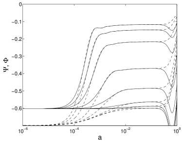
Figure 9: Evolution of $\Psi$ (solid lines) and $\Phi$ (dashed lines) in the presence of the Cardassian fluid (case III). From bottom to top, $k=0.00024,0.0012,0.0024,0.0060,0.012,0.036,0.048$ Mpc^-1.

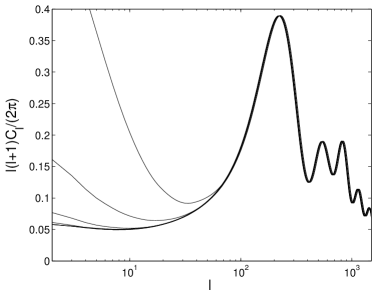
Figure 10: CMB spectra in the case III. Here $\nu=1$ and from bottom to up, $q=1,1.05,1.1,1.2,1.4,1.8$ and $2.6$.

The $\sigma$ in the first line is the total gauge-invariant shear stress which at late times gets a contribution only from $\sigma_{K}$. In the second line we have explicitly written down the relation of the shear stress to the density perturbation in the synchronous gauge, after $\delta_{K}$ in terms of $\delta_{c}$ from Eq.(23).

The stress appears during the Cardassian take-over period, and increases temporarily the magnitude of the metric perturbation $\Psi$. When the Cardassian density is beginning to dominate, the effect of stress is fading away. The integrated Sachs-Wolfe effect is stronger than in case I since now the effective matter source of the gravitational potentials is $\rho_{K}\delta_{K}$ instead of $\rho_{c}\delta_{c}$. The dip in the potential $\Psi$ may somewhat cancel the earlier contribution to the integrated Sachs-Wolfe effect, but the net effect is, as in case II, that the ISW again increases with increasing $q$. We show the evolution of gravitational potentials in Fig.9 for parameters $(q,\nu)=(1.5,1)$. The CMB spectra is plotted in Fig.10 for the same parameter choices as we did in case II. Choosing parameter values $\nu\neq 1$ seems to give similar results.

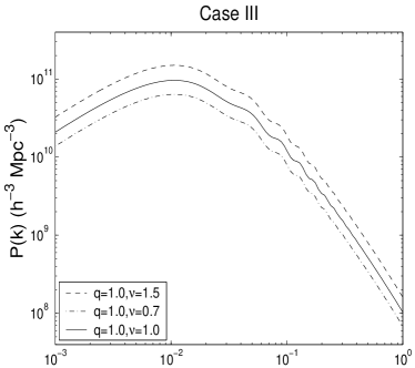
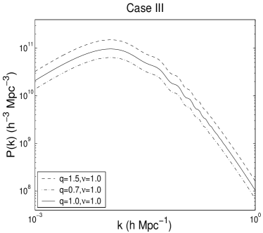
Figure 11: The total matter power spectra for different parameter values in the case III.

We plot the total matter power spectrum in Fig.11. Evolution of the linear overdensities seems to be similar as in the Case I. Thus the shape of the matter power spectrum is not as sensitive to the parameters $q$ and $\nu$ as the CMB spectrum at large scales.

Conclusions

We have attempted to describe modifications of the Friedmann equations in terms of a cosmological fluid with a priori unknown properties. We applied different assumptions on such a fluid to the representative case of the Cardassian model. In case I we assume that the fluid has no fluctuations and just provides a background for the evolution of the standard cosmological energy components.

A more physical assumption is considered in case $\rm{II}$ where we interpret the Cardassian energy density as that of an interacting dark matter. It is shown that then the requirement of a physically tolerable sound speed restricts the model to the unmodified polytropic Cardassian one, which is equivalent to the generalized Chaplygin gas model. These are known to predict damping of the matter power spectrumSandvik et al. (2004) and CMB spectrum inconsistent with observationsAmendola et al. (2003). Following ideas introduced in the Chaplygin gas literature Reis et al. (2003),Bento et al. (2004), we comment on the possibility to improve the results by modifying the fluid interpretation (of either Chaplygin gas scenario or the Cardassian expansion).

In case III we interpret the additional energy associated with the dark matter as arising from a modification to the general relativity. This is no longer compatible with perfectness of the fluid represented by $T_{\mu\nu}^{K}$. When Einstein equations are modified, we do not in general expect equality of the Bardeen potentials in the absence of anisotropic stress. If we then write the Einstein equations in the conventional form and take into account the modifications in the form of a fluid, it is generally found to be imperfect. This is also consistent withLue et al. (2004), where modified Friedmann equations are investigated under the assumption that the Birkhoff theorem is satisfied. Then also $\Psi$ and $\Phi$ are found to differ. In fact our approach to modified gravity in the case III coincides with the one inLue et al. (2004) at the scales they consider. Note that in the formulation of our case III, there is no problem of interpretation of the fluctuations in the present Universe. For the scales of interest, the dark matter perturbations evaluated in different gauges do coincide at late times. This is not true in the case II, as anticipated inGondolo and Freese (2003). Large scale structure in the limit $k\rightarrow 0$ in these models with assumptions equivalent to our case III was studied also inMultamaki et al. (2003).

In both cases we find that the late integrated Sachs-Wolfe effect is typically very large in the Cardassian models. For the fluid interpretation (case II) it is clear, also from the matter power spectrum, that the model is not compatible with observations unless one chooses parameters very close to the $\Lambda$CDM model. In the description of modified gravity (case III) the matter power spectrum is not as drastically distorted when $q,\nu\neq 1$, but it seems that the ISW effect could be used to rule out most of the parameter space also in this case. However, a detailed likelihood analysis is beyond the scope of the present paper.

Hannestad and Mersini-HoughtonHannestad and Mersini-Houghton (2004) have recently presented results of a more general investigation on the effects of new physics on the CMB spectrum. They also find that modifications of the late-time gravitational interactions can lead to a similar boost of the low-$\ell$ part of the spectrum as seen here in the Cardassian model for our cases II and III. It remains to be seen how generic this effect is and what constraints it puts on the equation of state for the dark energy.