Voids in a $\Lambda$CDM Universe

Abstract

We study the formation and evolution of voids in the dark matter distribution using various simulations of the popular $\Lambda$ Cold Dark Matter cosmogony. We identify voids by requiring them to be regions of space with a mean overdensity of $-0.8$ or less – roughly the equivalent of using a Spherical Overdensity group finder for haloes. Each of the simulations contains thousands of voids. The distribution of void sizes in the different simulations shows good agreement when differences in particle and grid resolution are accounted for. Voids very clearly correspond to minima in the smoothed initial density field. Apart from a very weak dependence on the mass resolution, the rescaled mass profiles of voids in the different simulations agree remarkably well. We find a universal void mass profile of the form $\rho(<r)/\rho(r_{\rm eff})\propto\exp[(r/r_{\rm eff})^{\alpha}]$ where $r_{\rm eff}$ is the effective radius of a void and $\alpha\sim 2$. The mass function of haloes in voids is steeper than that of haloes that populate denser regions. In addition, the abundances of void haloes seem to evolve somewhat more strongly between redshifts $\sim 1$ and 0 than the global abundances of haloes.

1 Introduction

Galaxy redshift surveys show that galaxies are not distributed uniformly. Instead, they form a complicated network around large regions that are almost empty, so-called voids. One of the most famous voids, in the region of Boötes, has a diameter of $\sim 50h^{-1}$Mpc, and was found by Kirschner et al (1981). Subsequent larger redshift surveys found more and more voids (for example Geller & Huchra 1989, da Costa et al 1994, Shechtman et al 1996, Einasto et al 1997, Plionis & Basilikos 2002). These surveys allowed studies of the properties of voids and of void galaxies (Einasto et al 1994, Lindner et al 1995 and 1996, El–Ad et al 1997, Müller et al 2000), but only recently have galaxy surveys become large enough to yield sufficient sample sizes for systematic studies (Hoyle & Vogeley 2002, 2004; Rojas et al 2003; Croton et al 2004).

For similar reasons, voids in cosmological N–body simulations have also been less well–studied. Early simulations of Cold Dark Matter (CDM) universes showed that large empty regions were generic (Icke 1984, Davis et al 1985), and larger more recent simulations (e.g., Jenkins et al 1998) have provided a clearer picture of the ‘void hierarchy’ (Van de Weygaert & Van Kampen 1993, Sheth & Van de Weygaert 2004). Detailed studies of the properties of voids in the dark matter distribution are now becoming increasingly common (Little & Weinberg 1994, Gardner 2001, Schmidt et al 2001, Gottlöber et al 2003, Patiri et al 2004).

Peebles (2001) noted that the properties of CDM voids and of the galaxies inside them formed a strong test for CDM. Subsequently, Mathis & White (2002) and Benson et al (2003) investigated properties of voids in semi–analytical models where mock galaxies are placed in dark–matter only simulations following physically motivated recipes.

One of the problems with voids and with studies of voids is that there is little agreement on how to define a void in the galaxy distribution. Are voids regions which are completely devoid of galaxies? Or can there be galaxies inside a void? If yes, how do void galaxies differ from their cousins that populate denser environments? And what is the spatial distribution of void galaxies within voids? Are they scattered throughout the void interior, or do they tend to pile up around the edges?

In models of galaxy formation within the context of hierarchical clustering, the galaxy distribution is determined by the underlying dark matter. Therefore, to understand void galaxies, it is important to define precisely what constitutes a void in the dark matter distribution. Dubinski et al (1992) argued that the spherical evolution model (Gunn & Gott 1972) provides a useful guide. In this model, initially underdense regions evolve from the inside out, in the sense that as mass makes its way outwards from the centre of the underdensity, a well–defined ridge begins to form around the region. The ridge is well–formed at a time when the density interior to it has a characteristic value (e.g. Fillmore & Goldreich 1984; Bertschinger 1985), and this, they argued, provides a natural and physically motivated definition of a void (also see Van de Weygaert & Van Kampen 1993; Friedmann & Piran 2001; Sheth & Van de Weygaert 2004). The main purpose of the present work is to present the results of a study which uses this definition of voids.

We will concentrate on voids in what has now become the standard cosmological model: a flat $\Lambda$CDM cosmology with $\Omega=0.3$. Rather than focusing on individual voids, or small sets of voids, we take a series of high–resolution N–body simulations done in sufficiently large cosmological volumes that a study the properties of ensembles of voids is justified. The set of simulations we use covers a wide range of cosmological volumes and resolutions. Thus, we are able to study detailed properties of voids such as the density run of the matter within them, as well as estimate their abundances.

This paper is organized as follows. In the following Section, we introduce the simulation set (§ 2.1) and the void finding algorithm (§ 2.2). In Section 3 we study the visual appearance of voids (§ 3.1), the void volume function (§ 3.2), the correspondence between voids and minima in the initial density field (§ 3.3), density profiles of voids (§ 3.4), the mass function of haloes in voids (§ 3.5), and the spatial clustering of voids (§ 3.6). Section 4 summarizes our findings.

2 Finding Voids in Cold Dark Matter Universes

2.1 The Simulations

We use of a set of N–body simulations done by, or in collaboration with, the Virgo Supercomputing Consortium. The simulations model regions of different sizes and have different mass resolutions. In the naming conventions of the Virgo Consortium, the simulations are:

1. The $\Lambda$CDM GIF simulation (Jenkins et al 1998; Kauffmann et al 1999), with $256^{3}$ particles in a cubic volume of size $(141.3\,h^{-1}\,$Mpc)³.

2. The $\Lambda$CDM GIF2 simulation (Gao et al 2003), with $400^{3}$ particles in a cubic volume of size $(110\,h^{-1}\,$Mpc)³. The mass resolution of this simulation is ten times better than that of the GIF simulation.

3. The $\Lambda$CDM VLS simulation (Jenkins et al 2001; Yoshida et al 2001; Menard et al 2003), with $512^{3}$ particles in a cube of volume $(479\,h^{-1}$ Mpc)³. This simulation has the same mass resolution as the largest boxes in Jenkins et al (1998) but is eight times their volume.

4. The $\Lambda$CDM Hubble Volume simulation (Evrard et al 2002), with $1000^{3}$ particles in a $(3000\,h^{-1}\,$Mpc)³ cube. Despite the relatively low mass resolution of this simulation, its size makes it extremely useful for studying the largest possible voids.

We note a difference in the initial power spectra for these simulations. The initial condition for the GIF simulation was generated using the Bond & Efstathiou (1984) transfer function whereas for the other simulations the transfer function computed by CMBFAST (Seljak & Zaldarriaga 1996) for the LCDM model was used. Table 1 provides a few more details about the simulations; in the following, we will refer to them as GIF, GIF2, VLS, and HV.

Run	$n_{p}$	$l$ [$h^{-1}$ Mpc]	$m_{p}[10^{10}\,h^{-1}\,M_{\odot}]$
GIF	$256^{3}$	141.3	1.4
GIF2	$400^{3}$	110	0.2
VLS	$512^{3}$	479	6.9
HV	$1000^{3}$	3000	224.8

Table 1: Parameters of the simulations used in this work. All runs have $\Omega_{m}=0.3$, $\Lambda=0.7$, $n=1$, $\sigma_{8}=0.9$, $h=0.7$.

Figure 1: File http://lahmu.phyast.pitt.edu/$\sim$colberg/voids/criteria.gif – Merging criteria for proto–voids: (a) Void 2 lies fully inside void 1 and thus belongs to void 1. (b) Void 2’s center lies inside void 1; the resulting void consists of void 1 plus the additional volume of void 2 that lies outside of void 1. (c) Void 2’s center lies outside of void 1, but the region of overlap is large enough to make the algorithm merge the two voids: ’x’ is longer than both ’y’ and ’z’. (d) If void 2 was merged with void 1 then the algorithm will not look whether it also overlaps with void 3.

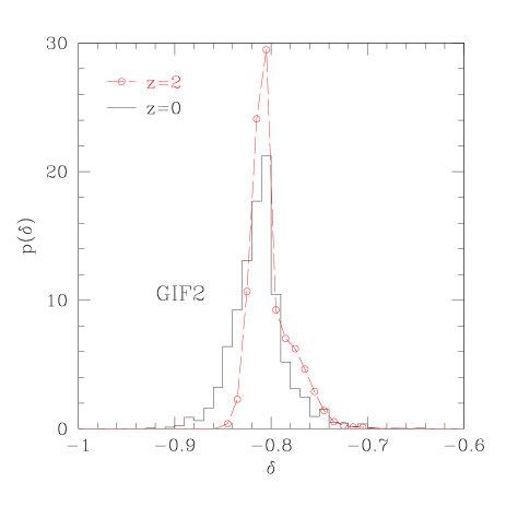
Figure 2: Distribution of (merged) void overdensities in the GIF2 simulation at redshifts $z=0$ (solid histogram) and 2 (connected circles). The overdensities scatter around the value of -0.8 used for the selection of the proto–voids (see description of void finding algorithm for explanation and discussion).

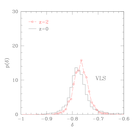
Figure 3: Distribution of (merged) void overdensities in the VLS simulation at redshifts $z=0$ (solid histogram) and 2 (connected circles). The overdensities scatter around a value of slightly less than -0.8 used for the selection of the proto–voids (see description of void finding algorithm for explanation and discussion).

2.2 The Void Finding Algorithm

A number of void-finding algorithms have been proposed (Kauffmann & Fairall 1991, Kauffmann & Melott 1992, El-Ad & Piran 1997, Aikio & Mähönen 1998, Hoyle & Vogeley 2002). Most look for empty spherical or cubical regions, which are then merged following some recipe. For the galaxy distribution, the decision to merge or not is slightly ad hoc. Our task is somewhat easier, because we are only searching for voids in the dark matter distribution, and we have a dynamically based model to use as a guide.

Our void finding algorithm is a variant of the one advocated by Aikio & Mähönen (1998). It is based on the assumption that voids are primordial negative overdensity perturbations that grew gravitationally and have reached shell–crossing at present time. At shell-crossing, the comoving radius of a perturbation is $1.7$ times larger than it was initially, so that the object has a density contrast of $-0.8$ (see Blumenthal et al. 1992, Dubinski et al. 1993). (Strictly speaking, these numbers are correct for an Einstein de-Sitter cosmology. But the dependence on cosmology is weak, and so we ignore it.) Our algorithm looks for such regions in the simulations. To be more precise, it performs the following steps:

1. The simulation particles are binned on a three–dimensional mesh using a nearest gridpoint scheme. We have checked that the choice of the grid size does not influence the locations and sizes of the voids, provided the smallest voids have radii of at least three cells.

2. The grid is smoothed adaptively, using 20 particles for the smoothing kernel. A fixed smoothing filter, for instance a Gaussian of some radius, smoothes the relatively large underdense regions nicely but washes out the smaller, highly clustered regions. As noted in the previous section, previous studies indicate that voids have well-defined steep edges which a fixed smoothing would wash out. The adaptive smoothing ensures that only regions with small particle numbers are heavily smoothed.

3. Local minima in the particle distribution are found, and spheres of varying radii are centred on these minima. The overdensity within these spheres is computed. The largest sphere within which the overdensity is $-0.8$ (or slightly smaller) is added to our list of void building blocks.

4. In principle, the entire underdense volume in a simulation box forms one big interconnected void: collapsed haloes form very small islands of matter surrounded by a vast underdense ocean (recall that collapsed haloes are much denser than the background, so they occupy only a small fraction of the volume). We divide this underdense ocean up into smaller voids that we require to either be spherical or ellipsoidal, or to have any other irregular shape, provided that they do not consist of two (or more) regions connected by thin tunnels. To avoid dumbbell–shaped configurations, the spherical void building blocks are merged using the following criteria (c.f. Figure 1):

   1. Any sphere which lies fully inside another is eliminated from the list.

   2. Any smaller sphere whose centre lies within a larger sphere is considered to be part of the larger volume; the void then contains the volume of the first sphere plus the additional volume of the second sphere. The overdensity of the resulting void is computed using its volume and the matter it contains.

   3. A sphere whose center lies outside the boundary of another sphere is considered to be part of the other if the following requirements are met. First, the two spheres must overlap. Second, the line which connects the centers of the two spheres is divided into three segments. A central part, which lies within the volume of intersection of the two spheres, and the two ends which do not. If the central segment is longer than one of the other two, the two spheres are considered to be part of the same void.

   4. If a sphere overlaps with another sphere the merging algorithm will not look for more overlaps. Thus, two large voids will never be connected by a thin bridge because the algorithm places a small sphere in between them only into one and not into both voids. This way, dumbell–shaped configurations are not possible.

Our void finder is analogous to the spherical overdensity method for dark matter haloes (Lacey & Cole 1994). We compute the center of each void by taking the volume–weighted average of the centers of its constituent spheres. By construction, voids need not be spherical, and we do not attempt to quantify the geometric shapes of the voids any further (for a discussion of this subject see Van de Weygaert & Van Kampen 1993 and references therein). Instead, we compute an ‘effective’ radius by taking the radius of a sphere whose volume is equal to that of the void. The effective radius has no deeper physical meaning but it is quite useful to get some idea of how big a void actually is. But note that in the spherical evolution model, the initial spherical region from which the void grew differs from this effective radius by a factor of $(1+\delta)^{1/3}$.

By running our algorithm on the simulated particle distributions at different epochs, we obtain void samples at a range of redshifts. We only consider voids whose radii are four times larger than the scale of the void–finder grid. Table 2 summarizes our results. The void radii/sizes in the different simulations are discussed in more detail in Section 3.2.

Figures 2 and 3 show the overdensities of the (merged) voids in the GIF2 and VLS simulations, respectively, at redshifts $z=0$ and $z=2$. The distributions scatter nicely around the value $\delta=-0.8$, with the peaks of the GIF2 and VLS distributions slightly above or below $\delta=-0.8$, respectively. This slight difference is due to the somewhat coarser grid of the VLS simulation.

Run	$z$	$r_{min}$	$r_{max}$	$n$
		[$h^{-1}$ Mpc]	[$h^{-1}$ Mpc]
GIF	0	1.2	32.1	5460
	1	1.2	16.5	8597
	2	1.2	9.0	5564
	3	1.2	4.3	1660
GIF2	0	0.7	19.8	7605
	1	0.7	14.3	14331
	2	0.7	6.3	21835
	3	0.7	4.3	13957
VLS	0	3.5	33.2	46405
	1	3.5	15.2	45592
	2	3.5	9.1	11730
	3	3.5	5.5	1063
HV	0	10.0	55.9	77726

Table 2: Void samples from the simulation sets. $r_{min}$ is the lower threshold for the void samples; $r_{max}$ is the effective radius of the largest void in the sample; $n$ denotes the total number of voids larger than $r_{\rm min}$ in our sample.

3 Voids in a $\Lambda$CDM Universe

3.1 Visual Impression

High–resolution N–body simulations contain a large number of three-dimensional objects. The appearance of these objects is usually illustrated by plotting the smoothed or unsmoothed particle distribution from a narrow slice through the simulation volume. However, projection effects can make objects seem to lie in the wrong places. What is more, images of smoothed density distributions are usually plotted using a logarithmic scale which tends to emphasize the matter between the haloes over the haloes themselves. (If a linear scale is used, most of the image would be relatively featureless, except for a few tiny specks that represent the haloes.) We will use a logarithmic scale in what follows, but it is important to keep this caveat in mind when looking at the images.

Figure 4: File http://lahmu.phyast.pitt.edu/$\sim$colberg/voids/GIF2_LCDM_voids_V2.jpg – A slice of thickness $10\,h^{-1}$ Mpc through the GIF2 simulation. The dark matter was smoothed adaptively, and the resulting density field is shown using a logarithmic colour scale. Circles show the effective radii of each void and are drawn to guide the eye (see main text for a more detailed description of how voids whose centers lie inside and outside the slice are represented). Numbers refer to a few points that have to be made about the plot (for more details see the main text): (1) Voids are shown as circles but in reality, they are not spherical. These three large voids do not overlap in our void catalog.(2) This part of an underdense region is not covered by any of the voids in this image because they are drawn as circles. In reality, it is part of the large void right above it. (3) Smaller voids seem to lie inside bigger ones. This is due to a combination of projection effects and of the fact that we draw voids as circles. The same goes for large haloes in voids. In the image, we have marked some of those voids that seem to be contained inside the larger void. (4) Regions that, on larger scales, are more overdense contain mostly small voids. (5) There are some small haloes inside voids. We have marked some of the small haloes inside the large void.

Figure 4 shows a slice of thickness $10\,h^{-1}$ Mpc – about one tenth of the full box size – through the GIF2 simulation. The dark matter was smoothed adaptively, and the density distribution was plotted using a logarithmic colour scale. The circles superimposed on the density field are centred on the centers of those voids that intersect this slice. For voids whose centers lie inside the slice we plot a circle with a radius equal to the effective radius. For voids whose centers lie outside the slice we determine the size of the overlap between the slice and the void that we represent as a sphere. We then plot a circle whose radius corresponds to the radius of the circle that is defined by the intersection of the sphere with the outer edge of the slice. The figure illustrates that the effective radii defined above correspond quite nicely to the visual impression of voids’ sizes. We added a few numbers to the image at locations that require some attention: (1) For reasons of simplicity, voids are shown as circles. In reality, they are not spherical. Thus, these three large voids do not overlap in the void catalog. (2) There is a small region here, which is underdense but not covered by any of the voids in this image. This effect is also due to the fact that we draw voids using circles. In reality, this underdense region is part of the large void right above it. (3) Smaller voids seem to lie inside bigger ones. This does not actually happen in our void catalogue. In the image, it is due to a combination of projection effects and of the fact that we draw voids as circles. Larger haloes also do not lie inside voids but are merely projected on top of them. It is worth noting that as a result of projection effects, if the centers of some of the larger voids lie close to the edge of the slice, they appear to be much larger than the particle distribution in the slice would have indicated. (4) Note how regions that are more overdense do not contain many large voids but, instead, mostly small ones. (5) There are some small haloes inside voids as is clearly visible in the center of this very large void.

Figure 5 shows the growth of the three largest voids in the GIF simulation. We are plotting a slice of thickness $10\,h^{-1}$ Mpc. However, in this plot, we center the region we are plotting on the $z=0$ position of each void. The evolution of the voids is quite interesting and it seems to follow the general picture outlined above: Even though the actual void shapes are not spherical, the voids grow from the inside, expanding outwards. Also note the presence of a very large void in the left–most column. This void has almost the size of the largest void in the VLS simulation.

Figure 5: File http://lahmu.phyast.pitt.edu/$\sim$colberg/voids/GIF_LCDM_void_mosaic_bw_V2.jpg – The largest voids in the GIF $\Lambda$CDM simulation. Each set of slices shows a $40\times 40\times 10$ ($h^{-1}$ Mpc)³ volume centred on one of the three largest voids. The sequence from top to bottom shows each void at $z=0$, 1, 2, and 3. The colour coding is the same for all voids and redshifts. At $z=0$, the three voids have effective radii of 32.1 $h^{-1}$ Mpc (leftmost column), 18.9 $h^{-1}$ Mpc (middle column), and 18.7 $h^{-1}$ Mpc (rightmost column).

3.2 The Void Volume Function

$z$	$f$
0	61.2%
1	27.6%
2	9.2%
3	2.7%

Table 3: Void volume fraction in the GIF2 simulation for a range of redshifts.

Table 3 shows the fraction of the simulation volume occupied by voids with radii larger than $r_{\rm min}$ in the GIF2 simulation. The volume fraction grows by approximately a factor of three between $z=3$ and 2, between $z=2$ and 1, and between $z=1$ and 0.

Figure 6: Cumulative volume functions of voids at $z=0$ in the GIF (dotted), GIF2 (dot–dashed), VLS (dashed), and HV simulations (dot–dot–dot–dashed).

Figure 7: Evolution of the the cumulative void volume fraction in the GIF2 simulation at $z=0$ (solid), $z=1$ (dotted), $z=2$ (dashed), and $z=3$ (dot–dashed).

Figure 8: Differential void volume function of voids in the GIF2 simulation at $z=0$.

Figure 9: Fraction of total void volume filled by voids of effective radius $r_{eff}$ or less in the GIF2 simulation at $z=0$. See text for discussion.

Figure 6 shows the number density of voids larger than a given volume $V$, as a function of $V$, at $z=0$ in the four simulations. The very big GIF void is clearly visible in this plot. It is almost as large as the largest voids in the much larger VLS simulation. The steps visible at small $V$ result from the discreteness of the grid. The agreement between the different simulations is really quite good. Of course, the Hubble Volume simulation contains by far the largest voids.

Figure 7 shows how the cumulative volume function in the highest resolution simulation (GIF2) evolves. The evolution is smooth, and the volume functions of different redshifts cross each other. For example, there are more voids of volume 100 ($h^{-1}$Mpc)³ at $z=1$ than at $z=0$. This growth of voids is analogous to the hierarchical growth of haloes. As time progresses, smaller haloes merge with one another to form larger haloes. Here, smaller voids expand and merge with other voids to form larger ones. (We did not attempt to use our void catalogs to construct void merger trees.) This plot reflects what we have shown earlier in the three sets of panels in Figure 5.

In Figure 8 we plot the differential void volume function of voids in the GIF2 simulation at $z=0$. It is interesting to note that the distribution does not have a peak. When expressed as a function of $1.7/\sigma(m,z)$, the halo mass function is reasonably well fit by a universal form that is independent of redshift and power spectrum (Sheth & Tormen 1999; Sheth, Mo & Tormen 2001; Jenkins et al 2001). However, a similar rescaling of the void function (using $2.8/\sigma(m)$ – see Sheth & Van de Weygaert 2004), does not yield a universal curve. The failure to find a universal form contradicts excursion–set models of the sort that describe halos quite well, but is not in disagreement with models based on peaks in Gaussian random fields (Sheth & Van de Weygaert 2004).

For the GIF2 simulation at $z=0$, in Figure 9 we plot the fraction of the total void volume filled by voids of effective radius $r_{eff}$ or less as a function of that radius. It is quite instructive to see that around half of the void volume is already filled at a radius of around 1.3 $h^{-1}$ Mpc, and voids with an effective radius of 2.5 $h^{-1}$ Mpc or less fill 90 percent of the void volume. In other words, even though the largest voids leave the strongest visual impression in images like Figure 4, they only account for a small fraction of the total void volume.

It is not straightforward to compare these findings with results from investigations of voids in galaxy catalogues. This is partly because of the difference in the void finding algorithms and mainly because of the fact that galaxies are quite sparse tracers of the underlying density field. On a qualitative level, our void size distribution agrees well with observed voids. For example, Hoyle & Vogeley 2004 report void sizes comparable to our largest voids (the smallest voids they construct have radii of 10 $h^{-1}$ Mpc), with the numbers of voids steeply dropping with increasing radius.

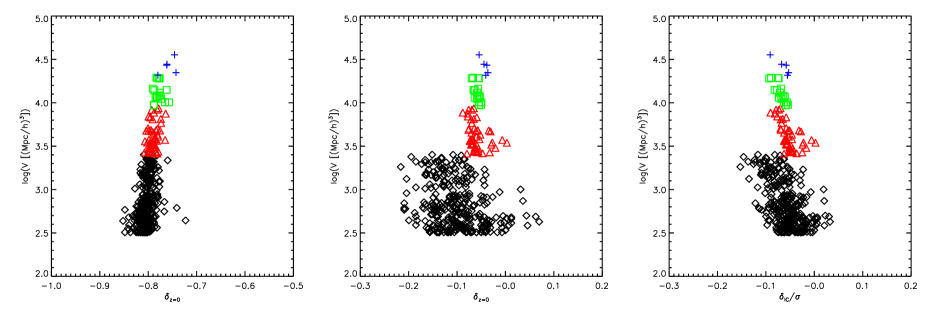
Figure 10: Left–most panel: Void volumes versus void overdensities at $z=0$ in the GIF simulation. Center panel: Voids in the smoothed initial density field (GIF simulation). Plotted is the void volume at $z=0$ as a function of the overdensity $\delta$ of the associated trough in the initial conditions. Different symbols show different smoothing scales: 2.5 $h^{-1}$ Mpc (diamonds), 5.0 $h^{-1}$ Mpc (triangles), 7.5 $h^{-1}$ Mpc (squares), and 10.0 $h^{-1}$ Mpc (crosses). Right–most panel: Voids in the smoothed initial density field (GIF simulation). Plotted is the void volume at $z=0$ as a function of the re–scaled overdensity $\delta/\sigma$ of the associated trough in the initial conditions. Different symbols show different smoothing scales: 2.5 $h^{-1}$ Mpc (diamonds), 5.0 $h^{-1}$ Mpc (triangles), 7.5 $h^{-1}$ Mpc (squares), and 10.0 $h^{-1}$ Mpc (crosses).

3.3 Voids In The Initial Density Field

Massive haloes in simulations are associated with higher peaks in the (smoothed) initial density field (Bardeen et al 1986; Colberg et al 2000; Sheth & Diaferio 2001). Voids are expected to form from initially underdense regions analogously to how clusters or haloes form from initially overdense regions. One might thus wonder if a similar correlation exists between voids and minima in the initial density field. We used the GIF simulations to study this correlation as follows.

In the spherical evolution model, the mass associated with a void is a measure of the initial comoving radius of the region from which it formed: $R=(3m/4\pi\bar{\rho})^{1/3}$. Therefore, one might expect the void mass to correlate most strongly with the depth of the initial underdensity from which it formed, when the initial field is smoothed on a scale $R(m)$. Since the voids in our sample enclose a large range of masses, we smoothed the initial ($z=49)$ density field using a set of Top Hat filters: 2.5, 5.0, 7.5, 10.0 $h^{-1}$ Mpc. We identified the minima in each smoothed field. That is, we identified those grid cells which were less dense than all twenty six of their neighbouring cells. We then compared the comoving positions of the minima identified on a smoothing scale with the locations of those voids whose $z=0$ sizes correspond to $R(m)$ – recall how initially underdense regions grow by a factor of 1.7 until present time. If there was more than one minimum inside a void we picked the deepest one. The density inside that cell was identified with the overdensity $\sigma$ of the trough. This method is analogous to how Colberg et al 2000 located peaks for clusters. What is more, voids evolve by expanding but not by moving. Thus, one expects to find the void centers in the initial conditions close to the void centers at present time. In this way, we associated voids with minima in the initial field.

As it turns out, all voids larger than 4.25 $h^{-1}$ Mpc could be associated with a density minimum. It is interesting that associating a void with an initially underdense region does thus work much better than finding a peak for a cluster (see Colberg et al 2000).

In the left–most panel of Figure 10 we plot the void volumes at $z=0$ as a function of the void overdensities at $z=0$. The void overdensities scatter around the value of -0.8. Larger voids tend to be slightly less underdense. This is mainly due to the process of the merging of proto–voids. As will be seen in the following section, void density profiles rise very sharply towards the edges of the voids (see Figure 14). Thus, when a smaller void is merged onto a larger one – following the criteria outlines above – one basically adds mainly parts of the outer region of the smaller void. Once the overdendity of the resulting void is computed this void will have a slightly higher overdensity than the two original voids.

The center panel of Figure 10 shows the $z=0$ void volume as a function of the overdensities of the associated troughs in the initial conditions. As discussed above, we used a set of smoothing scales and grouped the voids into categories covered by the corresponding scale. In principle, for each void one would want to apply a smoothing scale that corresponds exactly to the void volume. Since we did not do that we end up with clearly visible steps in the plot.

If one re–scales overdensities of the associated troughs (compare Sheth & Diaferio 2001 for the analogous procedure for haloes) the plot gets tighter. The right–most panel of Figure 10 shows the $z=0$ void volume as a function of $\delta/\sigma$ of the associated troughs. The different sets are still visible but now they lie on top of each other.

3.4 Void Density Profiles

Navarro et al (1996) have argued that CDM haloes have a universal density profile. In this section, we argue that the same holds true for voids, in qualitatively agreement with Van Kampen & Van de Weygaert (1993).

Figure 11: Enclosed density in $z=0$ voids as a function of radius for the GIF (dotted line), GIF2 (dashed line), and VLS (dot–dashed line) simulations. For each simulation, the rescaled profiles of voids with radii larger than $5\,h^{-1}$ Mpc were averaged (i.e., radii and densities were scaled by the effective radius and the enclosed density at the effective radius, before averaging). In addition, the results from the $\Omega=1$ $\tau$CDM GIF simulation are shown (three dots–dashed line). Curves are truncated at small radii because of numerical resolution limits.

Using our samples from the GIF, GIF2, and VLS simulations, we have computed the mass profiles of voids, using the actual particles in the voids instead of the smoothed density grid (we found the difference was important). Because of the different lower thresholds of the samples, we only compute void profiles for voids that have effective radii of $5\,h^{-1}$ Mpc or more. Figure 11 shows the averaged enclosed density in $z=0$ voids as a function of radius. For each void, we re–scaled the length scales by dividing by the effective radius, and we re–scaled densities by dividing by the enclosed density at the effective radius. We truncated the profiles at small radii, where numerical resolution effects begin to dominate (these will be discussed in more detail below). For almost the entire range, the average density profiles of voids in the three simulation sets agree very well. We also computed density profiles for the $\Omega=1$ $\tau$CDM GIF simulation. These agree with the profiles of the $\Lambda$CDM simulations. This finding indicates that the form of void density profiles is indeed universal.

The different mass resolution of the three simulations affects the profiles in a systematic way: the higher the resolution, the lower the profile. This effect is strongest at small radii. The mass resolution also affects the centers of the voids. For example, in the VLS simulation, a single particle in a sphere of radius $1\,h^{-1}$ Mpc corresponds to an overdensity of $-0.8$. Therefore, we cannot resolve the density profiles in the innermost regions. If we plot the profiles all the way to the centers we find that the profiles all rise – individual particles contribute too much mass. Therefore, we truncate the profiles in the void centers. We cross–checked the effect of mass resolution by down–sampling the GIF2 simulation and producing void profiles. The down–sampled simulation shows the trend visible in Figure 11. Figure 11 is very encouraging: except for the effect of mass resolution, there are no systematic differences in the void samples.

Figure 12: Enclosed density profiles in the VLS simulation. The voids were divided into four samples with void radii between 5 and $10h^{-1}$Mpc (dashed-three-dots), 10 and $15h^{-1}$Mpc (dot dashed), 15 and $20h^{-1}$Mpc (dashed), and voids with radii larger than $20h^{-1}$Mpc (dotted). The radius and enclosed mass of each void was rescaled by the effective radius and the effective mass, and these rescaled profiles were averaged over all voids. We have truncated the curves at small radii because of numerical resolution limits of the simulations. Solid line shows equation (1), shifted downwards by a factor of two.

Figure 13: Cumulative density profiles for different void overdensity definition thresholds in the GIF simulation.

Figures 12, shows the scaled enclosed density profiles of voids in the VLS simulation. The curves lie fairly nicely on top of each other. The cumulative profile shown in Figure 12 is quite well described by

$$\rho(<r)/\rho(r_{\rm eff})=\frac{\exp[(r/r_{\rm eff})^{1.85}]}{2.5}\,.$$ (1)

The fits only start to deviate somewhat beyond $r/r_{eff}=1$. (Although the density run around halos is usually studied using the differential profile, void centers have fewer particles, so we have chosen to fit to the cumulative profile instead.) Our choice of an exponential profile is motivated by Van de Weygaert & Van Kampen 1993 who noted that an exponential profile provided a very good fit to their voids.

Figure 13 shows the density profiles of voids in the GIF simulation with a range of values for the mean void overdensity. As can be seen, varying the overdensity threshold in the range chosen here does not systematically alter the density profiles.

Figure 14: Density profiles of four voids from the GIF simulation. Solid and dashed lines show the density and enclosed density as a function of distance from the void center. Vertical line shows the effective radius of each void.

Figure 14 shows density profiles of four GIF voids going out to a distance of $50h^{-1}$Mpc from their centers. The void edges are marked with a small vertical line. Although there are some variations in the profiles, all voids have very sharp edges. The densities peak at the effective radius, and the enclosed densities rise above the threshold. This is consistent with the visual impressions of voids discussed earlier, where one sees that voids are very well defined by the haloes which populate their boundaries. It also agrees qualitatively with the results in Van de Weygaert & Van Kampen (1993). What is more, Benson et al (2003) and Hoyle & Vogeley 2004 see similar behaviour for voids outlined by the galaxy distribution in a semi-analytic galaxy formation model and in the 2dFGRS, respectively (see Figure 11 in Benson et al (2003) and Figure 4 in Hoyle & Vogeley 2004).

3.5 The Void Halo Mass Function

Gottlöber et al (2003) investigated the $z=0$ void halo mass function using a set of high–resolution simulations of individual voids. They find that both the normalization and the shape of the cumulative mass function are different from those of the non–void halo mass function. Their measurements are in qualitative agreement with models for this dependence by Mo & White (1996) and Sheth & Tormen (2002), although there are differences in detail. Also see Patiri et al (2004) who used the simulations run by Gottlöber et al (2003) to model mass functions in voids.

For our study of the mass function, we use the GIF2 simulation, which has the highest mass resolution. We identify haloes using a friends–of–friends (fof) group finder with a linking length of 0.2 times the mean interparticle separation, and require that haloes have at least 10 particles. At $z=0$, we find void haloes by picking those haloes whose centres–of–mass lie within a void. We then mark those particles that are in a void at $z=0$ and run the fof group finder on them at earlier redshifts. This means that we do not require that $z=0$ void haloes be located inside a void at earlier times. Our choice is dictated by the fact that the void volume fraction evolves rapidly (c.f. Section 3.2); choosing only haloes that are inside voids at early times would reduce the size of our high redshift halo samples significantly. Thus, what we are really showing is the mass function of the high-$z$ projenitors of halos which are in voids at $z=0$.

Figure 15: Mass function of haloes in the GIF2 simulation. Different curves show the mass function of all haloes, whatever their surrounding environment, and the mass function of those haloes whose particles lie in a void at $z=0$.

Figure 16: Ratios of the mass functions of haloes in the GIF2 simulation in different environments. The solid ($z=0/z=1$) and dot–dashed ($z=1/z=2$) and the dotted ($z=0/z=1$) and dashed lines ($z=1/z=2$) are for all haloes and to void haloes, respectively.

Figure 15 compares the mass function of all haloes with that of haloes whose particles lie in a void at $z=0$.The plot indicates that haloes that end up in a void at $z=0$ – probably located at the very edges of a void – at any fixed mass undergo slightly more evolution than haloes with the same mass elsewhere. Figure 16 shows this point a little bit more clearly by plotting the ratios of the mass fuctions shown in Figure 15 for $z=0/z=1$ and $z=1/z=2$. Note that if you look at all haloes, for small halo masses there are less haloes at later redshift ($z=0$) than at the earlier redshift ($z=1$).

The small simulation volume and the resulting modest halo sample sizes do not allow more detailed studies of this. We will re–address the void halo mass function in a later study that will make use of a much larger simulation.

3.6 The Spatial Distribution of Voids

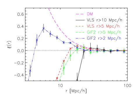
Figure 17: The two–point correlation function $\xi(r)$ for voids of radius $r>2$ Mpc/$h$ (from GIF2, dash three dots), $r>5$ Mpc/$h$ (dot dash from GIF2 and dashed from VLS), and $r>10$ Mpc/$h$i (solid line). The long dashed line shows the dark matter correlation function.

In this Section, we want to investigate the spatial clustering of voids in detail by computing the two–point correlation function of the voids. The correlation function of massive haloes depends strongly on halo mass (Mo & White 1996; Sheth & Tormen 1999), so it is interesting to see if voids show analogous trends.

To study a large range of void sizes, we measured the correlation function of voids centres in the VLS and GIF2 simulations. Figure 17 shows the results for voids with radii $R>2$ Mpc/$h$ (three dots dash) and $R>5$ Mpc/$h$ (dot dash) from GIF2, and with $R>5$ Mpc/$h$ (short dash) and $R>10$ Mpc/$h$ (solid) from VLS. At separations smaller than $\sim 2R$, the void correlation functions tend to $-1$. This is a consequence of volume exclusion: for the purposes of this statistic, voids are like hard spheres – they do not overlap. At larger radii, there is some evidence that the larger voids are slightly more clustered, consistent with a linear peaks-bias based model. (E.g., note the similarity between Figure 17 and Figures 2 and 3 in Sheth & Lemson 1999.) However, the scales on which volume exclusion effects are no longer important, and on which the linear bias model may apply are sufficiently large that the amplitude of the unbiased (dark matter) correlation function (long dash) is small. Hence, the actual amplitude of the void correlation function is never large compared to unity. This provides considerable justification for the accuracy of Van de Weygaert’s (2002) Poisson Voronoi based models of the matter distribution.

4 Conclusions

We studied the properties of voids in a set of large high-resolution N-body simulations of the $\Lambda$CDM cosmology. We defined voids as spherical or elliptical regions of space with a mean overdensity of $-0.8$. With this definition we found almost 80,000 voids with radii larger than $10h^{-1}$Mpc in the Hubble Volume simulation. Those voids fill the volume approximately uniformly.

The void volume functions of the different simulations agree well. The largest void in the HV simulation has a radius of $\sim 55.9h^{-1}$Mpc. It is quite interesting that this is fairly close to the size of the famous void in the region of Boötes found by Kirschner et al (1981).

The GIF simulation appears to harbor an abnormally large void, given the small size of the simulation box. There are more smaller voids at earlier times than at later times (Fig. 7). Claims that CDM cosmologies do not form large enough voids can thus be put to rest. In addition, as our voids are defined through their mean overdensity we also show that CDM voids do not contain too much matter.

Voids very clearly correspond to troughs in the smoothed initial density field (right–most panel of Fig 10). This point is particularly interesting in the light of Colberg et al (2000)’s result for the correspondence between clusters and peaks: They found that not all clusters could be associated with peaks. For voids, the idea that the initial density field contains the seeds of $z=0$ objects can be verified much more successfully.

When appropriately rescaled, voids appear to have a universal density profile (eq. 1). The void density profiles rise steeply at the edges of voids. Voids are thus very well defined in terms of their densities.

In agreement with the results reported by Gottlöber at al (2003) we find that the mass function of haloes in voids is different from that in regions of average density (Fig. 15). We also find that the mass function of haloes which end up in $z=0$ voids evolved somewhat more rapidly than the mass function of all haloes. However, even the simulation with the highest mass resolution in our set just barely reaches down to the mass range of void haloes. For a detailed investigation of formation times one would need simulations with an even higher mass resolution, such as those used by Gottlöber et al (2003). This is the subject of work in progress.

While there is some evidence that larger voids are slightly more clustered on scales larger than $\sim 20\,h^{-1}$ Mpc the actual amplitude of the void correlation function is very small. This finding supports the use of Poisson Voronoi based models of the matter distribution (Van de Weygaert 2002).

References

- [1] Aikio J., Mähönen P., 1998, ApJ, 497, 534
- [2] Benson A.J., Hoyle F., Torres F., Vogeley M.S., 2003, MNRAS, 340, 160
- [3] Bertschinger E., 1985, ApJ, 58, 1
- [4] Blumenthal G. R., Da Costa L, N., Goldwirth D. S., Lecar M., Piran T., 1992, ApJ, 388, 234
- [5] Bond J. R., Efstathiou G., 1984, ApJ, 285, 45
- [6] Colberg J. M., White S. D. M. MacFarland T. J., Jenkins A., Pearce F. R., Frenk C. S., Thomas P. A., Couchman H. M. P. (The Virgo Consortium), 2000, MNRAS, 313
- [7] Croton D. J., et al., astro-ph/0407537
- [8] da Costa L.N., Geller M.J., Pellegrini P.S., Latham D.W., Fairall A.P., Marzke R.O., Willmer C.N.A., Huchra J.P., Calderon J.H., Ramella M., Kurtz M.J., 1994, ApJ, 424, 1
- [9] Davis M., Efstathiou G., Frenk C.S., White S.D.M., 1985, ApJ, 292, 371
- [10] Dubinski J., Da Costa L, N., Goldwirth D. S., Lecar M., Piran T., 1993, ApJ, 410, 458
- [11] Einasto M., Tago E., Jaaniste J., Einasto J., Andernach H., 1997, A&AS, 123, 119
- [12] Einasto J., Saar E., Einasto M., Freudling W., Gramann M., 1994, ApJ, 429, 465
- [13] El-Ad H., Piran T., 1997, ApJ, 491, 421
- [14] El–Ad H., Piran T., da Costa L.N., 1997, MNRAS, 287, 790
- [15] Evrard A. E., MacFarland T. J., Couchman H. M. P., Colberg J. M., Yoshida N., White S. D. M., Jenkins A., Frenk C. S., Pearce F. R., Peacock J. A., Thomas P. A., 2002, ApJ, 573, 7
- [16] Friedmann Y., Piran T., ApJ, 548, 1
- [17] Gao L., White S. D. M., Jenkins A., Stoehr F., Springel V., astro-ph/0404589
- [18] Gardner J.P, 2001, ApJ, 557, 616
- [19] Geller M.J., Huchra J.P., 1989, Science, 246, 857
- [20] Goldberg D.M., Vogeley M.S., astro-ph/0307191
- [21] Gottlöber S., Lokas E., Klypin A., Hoffman Y., 2003, MNRAS, 344, 715
- [22] Hoyle F., Vogeley M. S., 2002, ApJ, 566, 641
- [23] Hoyle F., Vogeley M. S., 2004, ApJ, 607, 751
- [24] Icke V., 1984, MNRAS, 206, 1
- [25] Jenkins A., Frenk C. S., Pearce F. R., Thomas P. A., Colberg J. M., White S. D. M., Couchman H. M. P., Peacock J. A., Efstathiou G., Nelson, A. H. (The Virgo Consortium), 1998, ApJ, 499, 20
- [26] Jenkins A., Frenk C. S., White S. D. M., Colberg J. M., Cole S., Evrard A. E., Couchman H. M. P., Yoshida N., 2001, MNRAS, 321, 372
- [27] Kauffmann G., Fairall A. P., 1991, MNRAS, 248, 313
- [28] Kauffmann G., Melott A. L., 1992, ApJ, 393, 415
- [29] Kauffmann G., Colberg J. M., Diaferio A., White S. D. M., 1999, MNRAS, 303, 188
- [30] Kirshner R. P., Oemler A., Schechter P. L., Shectman, S. A., 1981, ApJ, 248, 57
- [31] Lacey C. Cole, S., 1994, MNRAS, 271, 676
- [32] Lindner U., Einasto M., Einasto J., Freudling W., Fricke K., Lipovetsky V., Pustilnik S., Izotov Y., Richter G., 1996, A&A, 314, 1
- [33] Lindner U., Einasto J., Einasto M., Freudling W., Fricke K., Tago E., 1995, A&A, 301, 329
- [34] Little B., Weinberg D. H., 1994, MNRAS, 267, 605
- [35] Mathis H., White S.D.M., 2003, MNRAS, 337, 1193
- [36] Menard B., Hamana T., Bartelmann M., Yoshida N., 2003, A&A, 403, 817
- [37] Müller V., Arbabi–Bidgoli S., Einasto J., Tucker D., 2000, MNRAS, 318, 280
- [38] Navarro J. F., Frenk C. S., White S. D. M., 1996, ApJ, 462, 563
- [39] Patiri S. G., Betancort–Rijo J. E., Prada F., astrop–ph/0407513
- [40] Peebles P. J. E., 2001, ApJ, 557, 495
- [41] Plionis M., Basilakos S., 2002, MNRAS, 330, 399
- [42] Reed D., Gardner J., Quinn T., Stadel J., Fardal M., Lake G., Governato F., astro-ph/0301270
- [43] Rojas R. R., Vogeley M. S., Hoyle F., Brinkmann J., astro-ph/0307274
- [44] Schmidt J. D., Ryden B. S., Melott A. L., 2001, ApJ, 546, 609
- [45] Seljak, U., Zaldarriaga M., 1996, ApJ, 469, 437
- [46] Shectman S. A., Landy S. D., Oemler A., Tucker D. L., Lin H., Kirshner R. P., Schechter P. L., 1996, ApJ, 470, 172
- [47] Sheth, R. K., Lemson G., 1999, MNRAS, 304, 767
- [48] Sheth R. K., Diaferio A., 2001, MNRAS, 322, 901
- [49] Sheth R. K., Van de Weygaert R., 2004, MNRAS, 350, 517
- [50] Van de Weygaert R., Van Kampen E., 1993, MNRAS, 263, 481
- [51] Yoshida N., Sheth R. K., Diaferio A., 2001, MNRAS, 328, 669