The VIMOS-VLT Deep Survey

We investigate the evolution of the galaxy luminosity function from the VIMOS-VLT Deep Survey (VVDS) from the present to $z\leavevmode\nobreak\ =\leavevmode\nobreak\ 2$ in five ($U$, $B$, $V$, $R$ and $I$) rest-frame band-passes. We use the first epoch VVDS deep sample of 11,034 spectra selected at $17.5\leq I_{AB}\leq 24.0$, on which we apply the Algorithm for Luminosity Function (ALF), described in this paper. We observe a substantial evolution with redshift of the global luminosity functions in all bands. From $z\leavevmode\nobreak\ =\leavevmode\nobreak\ 0.05$ to $z\leavevmode\nobreak\ =\leavevmode\nobreak\ 2$, we measure a brightening of the characteristic magnitude M^∗ included in the magnitude range $1.8-2.5$, $1.7-2.4$, $1.2-1.9$, $1.1-1.8$ and $1.0-1.6$ in the $U$, $B$, $V$, $R$ and $I$ rest-frame bands, respectively. We confirm this differential evolution of the luminosity function with rest-frame wavelength from the measurement of the comoving density of bright galaxies ($M\leq M^{*}(z\leavevmode\nobreak\ =\leavevmode\nobreak\ 0.1)$). This density increases by a factor of around $2.6,2.2,1.8,1.5,1.5$ between $z=0.05$ and $z=1$ in the $U$, $B$, $V$, $R$, $I$ bands, respectively. We also measure a possible steepening of the faint-end slope of the luminosity functions, with $\Delta\alpha\leavevmode\nobreak\ \sim\leavevmode\nobreak\ -0.3$ between $z=0.05$ and $z=1$, similar in all bands.

1 Introduction

The luminosity function (LF) of field galaxies is a fundamental diagnostic of the physical processes that act in the formation and evolution of galaxies. The LF evolution is mainly determined by the combination of the star formation history in each galaxy and the gravitational growth of structures, through merging. These two different processes are better probed by the luminosity emitted in the blue and red rest-frame wavelengths, respectively. The relative contribution of these processes to the cosmic history is reflected in the LF evolution, which therefore is expected to be different as a function of rest-frame wavelength. Large deep redshift surveys, combined with multi-color imaging, are necessary to perform this measurement.

The local LF is now well constrained by the results of two large spectroscopic surveys: the Two-Degree Field Redshift Survey (2dFGRS; Norberg et al. 2002) and the Sloan Digital Sky Survey (SDSS; Blanton et al. 2003). These measurements of the local LF represent the local benchmark for all studies of the LF evolution. Up to $z\simeq 1$ the Canada-France Redshift Survey (CFRS; Lilly et al. 1995) represents a sample of 591 spectroscopic redshifts of galaxies, from which it was demonstrated that the global LF evolves with cosmic time. Lilly et al. (1995) showed that the evolution of the LF depends on the galaxy population studied. The LF of the red population shows few changes over the redshift range $0.05\leq z\leq 1$, while the LF of the blue population brightens by about one magnitude over the same redshift interval. Up to $z\simeq 0.6$, the Canadian Network for Observational Cosmology Field Galaxy Redshift Survey (CNOC2; Lin et al. 1999 ) and the ESO-Sculptor Survey (ESS; de Lapparent et al. 2003 ) derived the LFs per spectral type with spectroscopic redshift samples of $\sim 2000$ and 617 galaxies, respectively. They confirmed a steep faint-end slope of the LF for the blue galaxy types. At higher redshift, LF measurements based on photometric redshifts have been derived by, e.g., Wolf et al. (2003) up to $z<1.2$, Gabasch et al. (2004) up to $z<5$. Samples of Lyman-break selected galaxies have also been used to measure the LF at such high redshift $3<z<5$ (e.g., Steidel et al. 1999).

The VIMOS (VIsible Multi-Object Spectrograph) VLT (Very Large Telescope) Deep Survey (VVDS) is a deep spectroscopic survey conducted over a large area associated with multi-color photometric data (Le Fèvre et al. 2004a ). Because of its characteristics, the VVDS is very well suited for detailed studies of the LF evolution :

• the Universe is surveyed over more than 90% of its current age with spectroscopic redshifts, which allows us to measure the LF evolution in a coherent way within a single sample from $z=0.05$ up to high redshift;

• the spectroscopic targets are selected on the basis of a simple magnitude limit criterion, with no attempt to exclude stars or AGNs, or to select objects on the basis of their colors or morphology. Therefore, this selection minimizes any bias in sampling the galaxy population up to high redshift;

• the multi-color coverage allows us to span a large range of rest-frame wavelengths, related to different physical processes, and thus to derive the LFs in several rest-frame bands;

• the spectra can also be used to derive the LFs as a function of specific spectral properties.

In this paper, we focus on the deep fields of the VVDS, which are the VVDS-0226-04 field (Le Fèvre et al. 2005) and the VVDS-Chandra Deep Field South (CDFS; Le Fèvre et al. 2004b). The first epoch VVDS deep sample contains 11,034 spectra of objects selected at $17.5\leq I_{AB}\leq 24.0$. The first goal of the LF analysis is to characterize the statistical properties of the whole population. It is the first measurement that a theory of galaxy formation must account for, because it is free of any of the possible biases which can arise when the sample is split into different sub-samples according to various selection criteria (e.g., rest-frame colors, morphology, spectral properties). In this paper, we present the measurement of the evolution of the global LF up to $z=2$. To investigate the dependence of this evolution on the rest-frame wavelength, the global LFs are estimated in five rest-frame bands, which span the wavelength range 3600Å$\leq\lambda_{eff}\leq$ 7840Å.

The paper is organized as follows. In Section 2 we briefly present the VVDS Deep first epoch sample. In Section 3 we describe the target sampling rate and the spectroscopic success rate of our data. In Section 4 we discuss two points relevant to the estimate of the global LF with VVDS data. This estimate is performed with our LF tool named Algorithm for Luminosity Function (ALF), extensively described in the Appendix. In Section 5 we present our results, compared with other literature measurements in Section 6. Conclusions are presented in Section 7. This paper will be followed by an analysis of the evolution of the LF per spectral type (Zucca et al. 2005), and as a function of environment (Ilbert et al. 2005).

We use a flat lambda ($\Omega_{m}\leavevmode\nobreak\ =\leavevmode\nobreak\ 0.3$, $\Omega_{\Lambda}\leavevmode\nobreak\ =\leavevmode\nobreak\ 0.7$) cosmology with $h\leavevmode\nobreak\ =\leavevmode\nobreak\ H_{\rm 0}/100$ km s^-1 Mpc^-1. Magnitudes are given in the $AB$ system.

2 Data description

We consider the deep spectroscopic sample of the first epoch data in the VVDS-0226-04 and VVDS-CDFS fields.

McCracken et al. (2003) describe in detail the photometry and astrometry of the VVDS-0226-04 field acquired with the wide-field 12K mosaic camera at the Canada-France-Hawaii Telescope (CFHT). The deep field covers 1.2 deg² and reaches the limiting magnitudes of $B_{AB}\sim 26.5$, $V_{AB}\sim 26.2$, $R_{AB}\sim 25.9$ and $I_{AB}\sim 25.0$, corresponding to 50% completeness. These data are complete and free of surface brightness selection effects at $I_{AB}\leq 24.0$, corresponding to the limit of the VVDS spectroscopic sample. Apparent magnitudes are measured using Kron-like elliptical aperture magnitudes (Kron 1980 ), with a minimum Kron radius of 1.2 arcsec. They are corrected for the galactic extinction estimated at the center of the VVDS-0226-04 field. For a large fraction of the field we have also U band data, taken at the ESO 2.2m telescope and reaching a limiting magnitude of $U_{AB}\sim 25.4$ (Radovich et al. 2004 ).

For the VVDS-CDFS, we have used the EIS $I$-band photometry and astrometry (Arnouts et al. 2001 ) for our target selection, and the multi-color $U$, $B$, $V$, $R$, and $I$ photometric catalogue from the COMBO-17 survey (Wolf et al. 2004 ).

The VVDS redshift survey uses the high multiplex capabilities of the VIMOS instrument installed at the Nasmyth platform of Melipal of the VLT-ESO in Paranal (Chile). The spectroscopic observations were obtained during two runs between October and December 2002. The spectroscopic targets were selected from the photometric catalogues using the VLT-VIMOS Mask Preparation Software (VVMPS; Bottini et al. 2005). The spectroscopic multi-object exposures were reduced using the VIPGI tool (Scodeggio et al. 2005 ). The sample of spectroscopic redshifts obtained in the VVDS-CDFS is described in Le Fèvre et al. (2004b) and the sample obtained in the VVDS-F02 is described in Le Fèvre et al. (2005). A total of 11,034 spectra were acquired as primary targets in the two fields. The range of magnitude of the observed objects is $17.5\leq I_{AB}\leq 24.0$. The deep spectroscopic sample (VVDS-0226-04+VVDS-CDFS) consists of 6582+1258 galaxies, 623+128 stars and 62+9 QSOs with secure spectroscopic identification, i.e. quality flags 2, 3, 4 and 9 (flags 2, 3, 4 correspond to redshifts measured with a confidence level of 75%, 95%, 100%, respectively; flag 9 indicates spectra with a single emission line). 1439+141 objects have an uncertain redshift measurement, i.e. quality flag 1 (flag 1 corresponds to a confidence level of 50% in the measured redshift). 690+102 objects have no spectroscopic identification, i.e. quality flag 0. This sample covers $\sim 1750+450$ arcmin², with a median redshift of about 0.76. The 1$\sigma$ accuracy of the redshift measurements is estimated at $\sim$0.001 from repeated VVDS observations (Le Fèvre et al. 2005).

3 Treatment of unidentified sources

In the estimate of the luminosity function, we introduce a statistical weight $w_{i}$, associated with each galaxy $i$ with a secure redshift measurement. This weight corrects for the non-observed sources and those for which the spectroscopic measurement failed (unidentified sources). This method yields the best statistical estimate of the total number of galaxies with the same properties as galaxy $i$, in the full field of view sampled by the spectroscopic data. The statistical weight $w_{i}$ is the product of :

• the weight $w_{i}^{TSR}$, inverse of the Target Sampling Rate (hereafter TSR). The TSR is the fraction of objects in the photometric catalogue that have been spectroscopically targeted. It can be a constant or a function of a number of parameters according to the strategy adopted in selecting the spectroscopic targets.

• the weight $w_{i}^{SSR}$, inverse of the Spectroscopic Success Rate (hereafter SSR). The SSR is the fraction of the spectroscopically targeted objects for which a secure spectroscopic identification has been obtained. In this paper, the LFs are computed using galaxies with secure redshift measurements, i.e. with spectroscopic quality flag 2, 3, 4 and 9. The SSR is the ratio between the number of objects with high quality flag 2, 3, 4 and 9 and the total number of spectra (quality flags 0, 1, 2, 3, 4 and 9). The correct estimate of the SSR is not trivial, because it can be a function of a large number of parameters, like, for example, magnitude, surface brightness, redshift and spectral type of the objects.

3.1 The TSR and its associated weight $w^{TSR}$

The VVDS strategy in selecting spectroscopic targets has been to select targets quasi-randomly from the photometric catalog, thus minimizing any bias in sampling the galaxy population. In the random selection process, the VVMPS tool (Bottini et al. 2005) uses the information about the size of the objects in order to maximize the number of slits per VIMOS pointing. As a consequence, the final spectroscopic sample presents a bias with respect to the photometric one, with large objects being under represented (see Bottini et al. 2005, for a discussion). The parameter used by VVMPS to maximize the number of slits is the x-radius, which is the projection of the angular size of each object on the x-axis of the image, corresponding to the direction in which the slits are placed. The x-radius is defined as x-radius=$(n+0.5)\times 0.204$, where 0.204 is the pixel size of the image expressed in $arcsec$ and $n$ is an integer corresponding to the size of the object in pixels. The TSR in the VVDS-0226-04 is shown as a function of the x-radius in the top panel of Fig.1. The TSR runs from $\sim 25$% for the smallest objects, to $\sim 10$% for the largest ones. As shown in the bottom panel of Fig.1, a large fraction of the total population ($\sim 75$%) is targeted with $TSR\sim 25$%. The under-sampling of the largest objects (x-radius $>$ 1.7) concerns less than $4$% of the total population, targeted with $TSR<15$%. Since the x-radius is the only parameter used to maximize the number of slits, the correction to be applied in order to correct for this bias is well defined and corresponds to using the weight $w_{i}^{TSR}=1/TSR(r_{i})$, where $r_{i}$ is the x-radius of the galaxy $i$.

Figure 1: Top panel: Target Sampling Rate as a function of the x-radius for the VVDS-0226-04 field. Bottom panel: x-radius distribution in the VVDS-0226-04 photometric catalogue at $17.50\leq I_{AB}\leq 24.0$.

3.2 The SSR and its associated weight $w^{SSR}$

Figure 2: Redshift distributions normalized to unity for each spectroscopic quality flag. For high quality flags 2, 3, 4, we show both the spectroscopic redshift distributions (dashed lines) and the photometric redshift distributions (solid lines) on the same area. For quality flags 0 and 1, we show only the redshift distribution estimated using the photometric redshifts.

Figure 3: Spectroscopic Success Rate as a function of redshift and per apparent magnitude bin. The associated weight is shown in the bottom of each panel.

The second weight to be used in the estimate of the LF is $w_{i}^{SSR}$, which is the inverse of the SSR. In Fig.16 of Le Fèvre et al. (2005) it is shown that the SSR is, as expected, a function of the $I_{AB}$ apparent magnitude. The SSR is greater than 90% for $I_{AB}<22.0$ and smoothly decreases down to $\sim 70$% in the faintest half a magnitude bin. In a first approximation, we could use this SSR distribution to derive $w_{i}^{SSR}$ as a function of the $I_{AB}$ apparent magnitude. However, this procedure implies that the objects with quality flags 0 and 1 belong to the same population of the objects with a secure spectroscopic identification (flags 2, 3 and 4). In particular, it implies that they have the same redshift distribution. The redshift distributions of galaxies with quality flags 4, 3 and 2 are shown in Fig.2. The distributions for each flag are clearly different, reflecting the fact that the quality flag is related not only to the signal-to-noise of the spectrum, but also to the number and the strength of identifiable spectral features. This suggests that the galaxies with quality flags 0 and 1 are likely to have a different redshift distribution. If that is the case, we would not be allowed to use $w_{i}^{SSR}$ as a function of magnitude only.

Therefore, making use of the multi-color properties of our sample, we have analyzed the distribution of photometric redshifts for the spectroscopic targets with flag 0 and 1. For this analysis we have used only a subset area of the VVDS-0226-04 field, with $\sim 1100$ spectra, in which, in addition to the $U$ photometry (Radovich et al. 2004 ), we have also $J$ and $K$ photometry (Iovino et al. 2005 ). We have restricted this analysis to the area with near-infrared data, since near infrared photometry allows us to estimate robust photometric redshifts at least up to $z\sim 2$ (see Bolzonella et al. 2005 for a detailed description of the method). A redshift probability distribution function (hereafter PDFz) is estimated for each object of the spectroscopic sample, using the photometric redshift code of Le Phare (Arnouts & Ilbert). We sum the normalized PDFz of all galaxies to estimate the expected redshift distribution (Arnouts et al. 2002 ). The stars are removed from the sample on the basis of their spectral identification if they have high quality spectroscopic flags, or on the basis of photometric criteria for the low quality flags (Bolzonella et al. 2005 ). The estimated redshift distribution of galaxies with quality flag 0 and 1 is shown in the bottom right panel of Fig.2. As expected, the estimated redshift distribution of the low quality flag galaxies differs from the redshift distribution of high quality flag galaxies, while the distributions of the photometric and spectroscopic redshifts for galaxies with flag $\geq$ 2 are consistent with each other.

We have then derived the SSR in various bins of apparent magnitude as the ratio between the estimated redshift distribution of high quality flag galaxies (quality flags 2, 3, 4, 9) and the estimated redshift distribution of all galaxies (quality flags 0, 1, 2, 3, 4, 9). This SSR is shown in Fig.3 as a function of redshift in four apparent magnitude bins for $I_{AB}\geq 22.5$ (at brighter magnitudes, the SSR is close to unity). Fig.3 clearly shows that the global SSR indeed decreases for fainter apparent magnitude bins and it varies significantly with redshift. The shape of the SSR is similar in all magnitude bins showing a maximum efficiency in the redshift measurement at $z\sim 0.7$ and a minimum SSR for $z<0.5$ and $z>1.5$. The dependence of the SSR on the redshift is related to the presence of the [O II] line, and/or the Balmer break within the observed spectral window 5500Å$\leq\lambda\leq$ 9500Å. The weight $w^{SSR}$ is shown in the bottom of each panel in Fig.3. The weight is binned in redshift in order to limit the statistical noise.

At $z>1.5$, the uncertainties on our weight are large due to the smaller number of galaxies, and to the uncertainties on the photometric redshifts at such redshifts (Bolzonella et al. 2005 ). We could also perform an other estimate of the weight at such high redshifts, using the spectroscopic redshifts of the spectra with quality flag 1 (50% of confidence level) and assuming that quality flag 0 objects have the same redshift distribution. Applying this method, we find SSR$\sim$20-30% above $z>1.5$, which provides a weight $\sim$2-3 times greater than the weight estimated with the photometric redshift method. The value of $w^{SSR}$ at $z>1.5$ will be refined in future analysis (Paltani et al., in preparation), using simulations and new spectroscopic VIMOS observations with a blue grism.

We apply the weights derived from this analysis to the whole sample, making the assumption that the subset area, from which they have been derived, is representative of our ability to measure a redshift. We assign to each galaxy, a weight $w_{i}^{SSR}$ that depends both on the apparent magnitude $m_{i}$ and on the redshift $z_{i}$ of the considered galaxy $i$.

To summarize, we have derived our statistical weights as the product of $w_{i}=w_{i}^{TSR}\times w_{i}^{SSR}=1/TSR(r_{i})\times 1/SSR(m_{i},z_{i})$. This weighting scheme allows us to correct for:

• the TSR, taking into account the small under-sampling of the largest objects in the target selection;

• the SSR, taking into account the dependence on the apparent magnitude and redshift.

4 ALF applied to the VVDS

We have measured the LF on the VVDS data, using our luminosity function VVDS tool, named Algorithm for Luminosity Function (ALF). The methods implemented in ALF are extensively described in the Appendix. In this Section we briefly discuss two points which are relevant for a better understanding of our treatment of the data in this paper.

4.1 Effect of the $w^{SSR}$ weight on the LF estimates

Figure 4: Comparison between the ‘unweighted’ LFs (solid triangles for 1/V_max, solid lines for STY) and our best LF estimates (‘weighted’) (open circles for 1/V_max, dotted lines for STY) in the $B$ rest-frame band. The best STY fits and the associated 90% error contours are shown as insets with the same symbols. We report in each inset the SDSS local estimate with open triangles.

As shown in Section 3, while the weight $w^{TSR}$ is fully understood and well established, the derivation of the weight $w^{SSR}$ is less direct and subject to more uncertainties. To quantify the effect of $w^{SSR}$ on our LF estimate, we have also derived an ‘unweighted’ LF, in which no correction for the SSR is applied (i.e. $w^{SSR}=1$). The ‘weighted’ and ‘unweighted’ LFs are shown in Fig.4, in the $B$ rest-frame band.

Since the galaxies with flag 0 and 1 can not be ignored in the LF estimate, the ‘unweighted’ LF is by definition a lower limit of the LF. However, given the relatively small fraction of galaxies with flag 0 and 1, the difference in the overall normalization of the two LFs is small. From Fig.4, we see that the main effect of $w^{SSR}$ is to steepen the slope of the ‘unweighted’ LF. In all the redshift bins, the parameter $\alpha$ of the weighted LF is smaller (i.e. steeper slope), by less than 0.2 up to $z=1.0$, by less than 0.3 in the two higher redshift bins. This effect is clearly expected, since the galaxies with flag 0 and 1, which are included in the LF estimate through the weight, are mainly faint galaxies close to our magnitude limit. Since $\alpha$ and $M^{*}$ are correlated, the steepening of the slope with the weight produces also a brightening of $M^{*}$, less than 0.25 up to $z=2$.

4.2 Estimate of the LF from a homogeneous galaxy population

Ilbert et al.(2004) have shown that the estimate of the global LF can be biased, mainly at its faint-end, when the band in which the global LF is measured is far from the rest-frame band in which galaxies are selected. This is because different galaxy types have different absolute magnitude limits, because of different k-corrections. In each redshift range, we avoid this bias in our estimates of the LF by using only galaxies within the absolute magnitude range where all the SEDs are potentially observable. We perform only the 1/V_max estimate on the whole absolute magnitude range. This estimator leads to an under-estimate of the LF in the absolute magnitude range fainter than this ‘bias’ limit (Ilbert et al. 2004), providing a lower limit of the LF faint-end.

5 Results

The global LFs are computed up to $z=2$ in the five standard bands $U$, $B$, $V$, $R$, $I$ ($U$ Bessel, $B$ and $V$ Johnson, $R$ and $I$ Cousins). The LFs are computed using the weighting scheme described in Section 3. The $U$-, $B$-, $V$-, $R$- and $I$-band LFs are displayed in Fig.5 and in Fig.6. In Fig.7, we plot the STY best estimate of $\alpha-M^{*}$, and the associated error contours. For each band and each redshift bin, the Schechter parameters and the corresponding one sigma errors measured with the STY estimator are listed in Table 1.

Figure 5: Estimate of the global LF in the $U$ band from $z=0.05$ to $z=2$. The estimate is derived using the weighting scheme described in Section 3. We adopt the following symbols for the various estimators: circles for the 1/V_max, triangles for the SWML, squares for the C⁺ and solid lines for the STY. The vertical short-dashed lines show the faint absolute magnitude limits considered in the STY estimate (see Section 4.2). In each panel, we show also the local LF derived by the SDSS (long dashed lines). The vertical dot-dashed line in the redshift bin 0.05-0.2, corresponds to the faint absolute magnitude limit surveyed by the SDSS.

Figure 6: Same symbols as in Fig.5, in the rest-frame band $B$ (upper-left), $V$ (upper-right), $R$ (lower-left) and $I$ (lower-right).

Figure 7: $M^{*}-\alpha$ error contours, at 90% confidence level ($2\Delta ln\mathcal{L}=4.61$), obtained with the STY estimator. The solid squares are the STY best estimates. Error contours are not drawn when one of the two values has been fixed (see text). When $\alpha$ is fixed, we estimate the range of allowed $M^{*}$ values, varying $\alpha$ between $\alpha=-2.0$ and $\alpha=-1.2$. When $M^{*}$ is fixed, we vary $M^{*}$ by 0.5 around the set value. The error contours are shown for the $U$, $B$, $V$, $R$ and $I$ band LFs from the left to the right panels, respectively. The panels from the top to the bottom correspond to the eight redshift bins, from $z=0.05$ to $z=2$. We report with open triangles the SDSS local values (the error bars are included inside the symbols).

5.1 Local LF at $z=0.1$

The local LF derived with the VVDS sample refers to the redshift bin [$0.05-0.2$]. The average redshift in this bin ($<z>\sim 0.14$) is directly comparable to the average redshift of galaxies in local surveys with a brighter limiting magnitude, like the SDSS ($<z>\sim 0.1$). Due to the bright apparent magnitude cutoff of the VVDS sample ($I_{AB}\geq 17.5$), the $M^{*}$ parameter of the STY fit in this redshift bin is essentially unconstrained. Therefore, we set the $M^{*}$ parameter to the local value derived by Blanton et al. (2003). The LFs of the SDSS are expressed in the bands ${}^{0.1}u$, ${}^{0.1}g$, ${}^{0.1}r$, ${}^{0.1}i$, ${}^{0.1}z$ (Fukugita et al. 1996 ) blue-shifted at $z=0.1$, which correspond roughly to the $U$, $B$, $V$, $R$, $I$ bands of our standard system. In order to check if the absolute magnitudes estimated in the SDSS band system and in our standard band system are comparable, we have estimated the absolute magnitudes in the filters ${}^{0.1}u$, ${}^{0.1}g$, ${}^{0.1}r$, ${}^{0.1}i$ and ${}^{0.1}z$ from the apparent magnitudes measured in the instrumental system (using the formulae A.1 and A.2 given in appendix A). The average difference between the absolute magnitudes computed in $B$, $V$, $R$, $I$ and in ${}^{0.1}b$, ${}^{0.1}v$, ${}^{0.1}r$, ${}^{0.1}i$ bands are less than 0.05. The difference is more significant in the $U$ band ($\Delta M\sim 0.25$). We have therefore converted $M^{*}_{SDSS}(^{0.1}u)$ to our band with the relation $M^{*}_{SDSS}(U)=M^{*}_{SDSS}(^{0.1}u)-0.25$. The local values of $\alpha$ and $\phi^{*}$, with $M^{*}$ set to the SDSS value, are listed in Table 1 and the LFs are shown in Fig.5 and Fig.6. Even if the volume surveyed by the VVDS in the first redshift bin is approximately one thousand times smaller than the volume surveyed by the SDSS, the estimates of the local LFs produced by the VVDS and the SDSS are in good agreement in the magnitude range in common to both surveys. However, in all the bands, the VVDS best fit slope is steeper than the SDSS slope. The larger difference is in the $B$ band, where it is formally significant at $\sim 3\sigma$ level ($\alpha_{SDSS}=-0.89\pm 0.03$ while $\alpha_{VVDS}=-1.09\pm 0.05$). In this band the VVDS slope is instead consistent with that derived by Norberg et al. (2002) from the 2dFGRS. Even if the number of objects in the VVDS is smaller than in the SDSS, the faint-end slope of the LF is better constrained by the VVDS because it samples the local galaxy population about 3-4 magnitudes deeper than the SDSS. The steeper slope observed in the VVDS cannot be due to the effect of the applied weights since also the ‘unweighted’ LF, which under-estimates the slope (see Section 4.1), has a steeper best fit slope than the SDSS ($\alpha_{VVDS}=-1.02\pm 0.05$ in the $B$-band). The inclusion of a fit for simple luminosity and number evolution in the LF estimate, using the maximum likelihood estimator proposed by Blanton et al. (2003), could also produce a flatter slope.

5.2 LF evolution up to $z=2$

Figure 8: Evolution with redshift of the ratio between the density of galaxies brighter than $M^{*}_{SDSS}(z=0.1)$ and the SDSS local value.

The VVDS allows us to quantify the galaxy evolution within a single sample and with the same selection function, over a wide redshift range. From $z=0.05$ up to $z=2$, the evolution of the bright part of the LFs is clearly evident from all non-parametric estimators shown in Fig.5 and Fig.6. It also appears to be a function of the considered rest-frame wavelength. This can be quantified using the Schechter parameters measured with the STY estimator, as done below.

To quantify the strength of the evolution with redshift, we have derived the density of galaxies brighter than the corresponding local value of $M^{*}$:

$$\rho(M<M^{*}_{SDSS})=\int_{-\infty}^{M^{*}_{SDSS}}\phi(M)dM,$$

where $M^{*}_{SDSS}$ is the local value estimated by Blanton et al. (2003). This measurement quantifies the global evolution of the bright part of the LFs, in shape and in normalization. In all bands and up to $z\leq 1$, $M^{*}_{SDSS}$ is brighter than the faintest limits used for the STY estimate. We have therefore limited this analysis to z $\leq$ 1, in order to avoid extrapolation of the LF beyond the last measured point. In Fig.8 we show the evolution with redshift of the ratio $\rho(M<M^{*}_{SDSS})/\rho_{SDSS}(M<M^{*}_{SDSS})$ for the five bands. As the figure clearly shows, the density evolution of bright galaxies is significantly dependent on the rest-frame wavelength, being stronger at shorter wavelengths. In the $U$ band, $\rho(M<M^{*}_{SDSS})$ increases continuously and becomes $\sim 2.6$ times greater than locally at $z=1.0$, while in the $I$ band this factor is only $\sim 1.5$ at $z=1$.

The evolution of the best fit $M^{*}$ as a function of redshift for the five bands is shown in the central panel of Fig.9. We find that the characteristic magnitude M^∗ of the whole population strongly evolves. Up to $z=1$, the slope can still be constrained reasonably well and we measure a brightening of $1.57\pm 0.26$, $1.48\pm 0.17$, $1.41\pm 0.22$, $1.49\pm 0.25$ and $1.45\pm 0.26$ magnitudes in the $U$, $B$, $V$, $R$ and $I$ rest-frame bands, respectively. Above $z=1$, the slopes are set to the $\alpha$ value obtained in the redshift bin $0.8\leq z\leq 1$ and we measure a brightening of about $2.0$, $1.8$, $1.4$, $1.3$, $1.2$ magnitudes up to $z=2$. When $\alpha$ is fixed, we estimate the range of allowed $M^{*}$ values, varying $\alpha$ between two extreme values of the slope, $\alpha=-2.0$ and $\alpha=-1.2$. We find a brightening included in the range $1.8-2.5$, $1.7-2.4$, $1.2-1.9$, $1.1-1.8$ and $1.0-1.6$ magnitudes in the $U$, $B$, $V$, $R$ and $I$ rest-frame bands, respectively. Also in this representation, the evolution is stronger in the bluer rest-frame bands. Since $M^{*}$ and $\alpha$ are correlated and we have some evidence that also $\alpha$ is changing with redshift (see below and upper panel of Fig.9), we have verified that the observed evolution in $M^{*}$ is not induced by the change with redshift of the $\alpha$ value. The bottom panel of Fig.9 shows the best fit $M^{*}$ parameters derived by setting the value of $\alpha$ to the VVDS local value over the entire redshift range. Also in this case, a significant and differential evolution of $M^{*}$ is seen, with $\Delta M^{*}\sim-1.7,-1.6,-1.2,-1.1,-1.0$ up to $z\sim 2$, in the $U$, $B$, $V$, $R$, $I$ bands respectively. The measurement of this brightening is slightly sensitive to the adopted weighting approach and it is also measured, at a similar level, with the ‘unweighted’ LFs (see Fig.4).

The upper panel of Fig.9 shows the best fit values of $\alpha$ as a function of redshift. The one sigma error bars on $\alpha$ take into account the correlation between $\alpha$ and $M^{*}$. The data suggest a steepening of the slope with increasing redshift. The measured variation of $\alpha$ between $z=0.05$ and $z=1$ is $\Delta\alpha\sim-0.3$, similar in all the bands.

Figure 9: Evolution in the five bands of the parameter $\alpha$ in the top panel and of the parameter $M^{*}$ in the second panel. The bottom panel shows the evolution of $M^{*}$ with the slope fixed to the VVDS local value.

Figure 10: Comparison between the CFRS and the VVDS global $B$-band LFs. The solid lines (STY) and the circles (1/V_max) correspond to the VVDS estimates. The vertical short-dashed lines are the faint absolute magnitude limits considered in the STY estimates. The long-dashed lines correspond to the CFRS estimate. The vertical dot-dashed lines correspond to the faint absolute magnitude limits surveyed by the CFRS.

6 Comparison with previous redshift surveys

6.1 Comparison with the CFRS survey

Lilly et al. (1995) have derived the global $B$-band LFs of the Canada-France Redshift Survey (CFRS) up to $z\sim 1$. The CFRS spectroscopic sample contains 591 redshifts of galaxies selected with $17.5\leq I_{AB}\leq 22.5$. The survey covers 125 arcmin² in five separated fields. The VVDS deep spectroscopic sample is surveying the galaxy population 1.5 magnitude fainter and the field of view is ten times larger than the CFRS. The comparison between VVDS and CFRS results in three redshift bins is displayed in Fig.10 (in the cosmology $\Omega_{m}=1$, $\Omega_{\Lambda}=0$, which was adopted in the CFRS analysis). The estimated LFs for the two surveys are in agreement up to the faintest absolute magnitude limits reached by the CFRS. The slopes of the VVDS are, however, steeper than the CFRS slopes (the difference is particularly significant in the redshift bin ]0.5-0.75]). The slopes estimated from the VVDS are clearly more robust, since the VVDS is 1.5 magnitudes deeper and contains 10 times more galaxies than the CFRS.

Figure 11: Comparison between the global $B$-band LFs derived with the HDF data (Poli et al. 2003) and with the VVDS data. The solid lines (STY) and the circles (1/V_max) correspond to the VVDS estimates. The vertical short-dashed lines are the faint absolute magnitude limits considered in the STY estimates. The long dashed lines correspond to the global LFs derived by Poli et al. (2003). The vertical dot-dashed lines correspond to the faint absolute magnitude limits surveyed by the HDF data.

6.2 Comparison with the HDF data

Poli et al. (2003) have derived the global $B$-band LFs from z = 0.4 up to z = 3.5, using a composite sample of 1541 I-selected galaxies down to $I_{AB}=27.2$ and 138 K-selected galaxies down to $K_{AB}=25$. The faintest galaxies of this composite sample are drawn from HDF North and South data. Data from two additional fields (the CDFS and the field around the QSO 0055-269), on which the K20 spectroscopic survey is based (Cimatti et al. 2002 ), have been added to constrain the bright-end of the LF. Given the faintness of this sample, most of the redshifts ($\sim 80\%$) are photometric redshifts. Poli et al. (2003) have derived the global $B$-band LF using the $I$-selected sample up to $z=1$ and the $K$-selected sample for $z\geq 1.3$. The HDF data survey the LF faint-end about 2-3 magnitudes fainter than the VVDS data. The LFs from Poli et al. (2003) and the corresponding VVDS LFs are shown in Fig.11 in three redshift bins. At $z>1.3$, Poli et al. (2003) have derived the LF in the redshift bin [1.3-2.5], that we compare here with our measurement in the redshift bin [1.3-2]. As shown in Fig.11, there is an excellent agreement in the bright part of the LF between the VVDS and the Poli et al. (2003) measurements, up to $z=2$. In the faint part of the LF, the slope estimated by Poli et al. (2003) is slightly steeper ($\Delta\alpha\sim 0.15$) than the slope estimated with the VVDS data in the redshift bin [0.4-0.7].

6.3 Comparison with the COMBO-17 survey

Wolf et al. (2003) have derived the LFs up to $z=1.2$ with a sample of $\sim$ 25,000 galaxies from the COMBO-17 survey. This sample is selected in the $R$ band ($R_{vega}\leq 24$). The redshifts are photometric redshifts derived from medium-band photometry in 17 filters. The Schechter parameters of the COMBO-17 global LF are available in the online material of the paper (Wolf et al. 2003). The comparison between the $B$-band global LFs of VVDS and COMBO-17 surveys is shown in the Fig.12 in five redshift bins up to z = 1.2.

The bright parts of the LFs appear to be roughly in agreement, although some significant differences are seen in a few redshift bins (see, for example, the redshift bins [0.4-0.6] and [0.8-1]). Given the errors on the $\alpha-M^{*}$ parameters reported by the two surveys, the overall LF shapes are not consistent with each other (see insets in Fig.12). Since the COMBO-17 sample is selected from the $R$ band, its global $B$-band LF could be affected by the bias described in Ilbert et al. (2004) at $z>0.5$. This bias introduces an overestimate of the LF faint-end at $z>0.5$ and could explain the significantly steeper slope measured by the COMBO-17 survey in the redshift bins [0.6-0.8] and [0.8-1]. Since $\alpha$ and $M^{*}$ are correlated, the same effect could also explain the differences seen in the bright part of the LF. These discrepancies can also be due to other reasons as, for example, a smaller fraction of very blue galaxies in the I-selected VVDS sample (in fact, the LF of the bluest galaxies has the steepest faint-end LF) or a bias in the COMBO-17 estimate due to their use of photometric redshifts. These possibilities will be better investigated through a comparison of the COMBO-17 and VVDS LFs for each galaxy type (Zucca et al. 2005), since such a comparison is much less affected by the bias discussed above (Ilbert et al. 2004).

Figure 12: Comparison between the COMBO-17 and the VVDS global $B$-band LFs. The solid lines and the points correspond to the VVDS estimates. The vertical short-dashed lines are the faint absolute magnitude limits considered in the STY estimates. The long dashed lines are the global LFs derived by Wolf et al. (2003). The vertical dot-dashed lines correspond to the faint absolute magnitude limits surveyed by the COMBO-17 data. The best estimated values for the $\alpha,M^{*}$ parameters measured by the VVDS are shown with solid squares in insets, and the associated 90% error contours with solid lines. The ($\alpha,M^{*}$) parameters given by COMBO-17 are the open stars, with error bars included inside the symbols.

7 Conclusions

We use the first epoch spectroscopic deep sample of the VVDS, with 11,034 spectra selected up to $I_{AB}=24$, to derive the global LF up to $z=2$ in the five bands $U$, $B$, $V$, $R$, $I$. The global LFs are measured using ALF and care is taken to remove the bias introduced by the difference of visibility of the different galaxy spectral types.

We observe a clear evolution of the global LF with redshift in all bands and we find that this evolution is significantly dependent on the rest-frame wavelength, being stronger at shorter wavelengths. The comoving density of the bright galaxies increases with redshift from $z=0.05$ up to $z=1$. This increase is by a factor $\sim 2.6$ in the $U$ band and becomes smaller for redder rest-frame wavelengths, with values of the order of $2.6,2.2,1.8,1.5,1.5$ in the $U$, $B$, $V$, $R$, $I$ bands, respectively.

In order to better distinguish the processes responsible of this evolution, we have studied the evolution with redshift of the Schechter parameters computed with the STY estimator. This analysis suggests a possible steepening of the slope with redshift. The observed change in $\alpha$ is $\sim-0.3$ from $z=0.05$ up to $z=1$, similar in all bands. This evolution has to be confirmed with the on-going second epoch VVDS data, which will allow us to decrease significantly the statistical errors on $\alpha$. This evolution of the global LF slope is expected because of the different evolutions observed for the different galaxy types (Zucca et al. 2005). In particular, since the LF of blue galaxies has a steep slope and evolves strongly with redshift (e.g., Lilly et al. 1995, Zucca et al. 2005), the relative contribution of the blue population to the global LF increases with redshift and could explain the steepening of the slope.

We also measure a significant brightening of the global LF with redshift. This brightening, parameterized as the change of the best fit value of $M^{*}$, is a function of the rest-frame wavelength. Compared to the local SDSS values, we obtain a brightening included in the range $1.8-2.5$, $1.7-2.4$, $1.2-1.9$, $1.1-1.8$ and $1.0-1.6$ magnitudes from $z=0.05$ up to $z=2$, in the $U$, $B$, $V$, $R$ and $I$ rest-frame bands. This tendency of a stronger brightening toward bluer rest-frame wavelengths is consistent with existing measurements at shorter and longer rest-frame wavelengths. In the rest-frame far-UV (1530 Å), Arnouts et al. (2005) measure a brightening $\Delta M^{*}\sim-2$ magnitudes up to $z=1$, stronger than our measurement in the $U$ band in the same redshift interval. In the near-IR, Pozzetti et al. (2003) measure an evolution consistent with a mild luminosity evolution both in the $J$ and $K$ bands with $\Delta M_{J}\sim-0.7$ and $\Delta M_{K}\sim-0.5$ at $z\sim 1$. This differential evolution of $M^{*}$ with wavelength is expected, since the rest-frame luminosity at different wavelengths probes different physical processes acting in galaxy formation and evolution. The fact that the brightening is stronger in the bluest bands suggests that most of the evolution of the global LFs up to $z=2$ is related to the star formation history, better probed with the luminosity measured at short rest-frame wavelengths. The luminosity density and star formation rate derived from the VVDS first epoch observations will be presented in Tresse et al. (2005). We will explore the evolution of the LFs per spectral types and as a function of the local environment in forthcoming papers (Zucca et al. 2005, Ilbert et al. 2005).

$\Omega_{m}$=0.3           $\Omega_{\Lambda}$=0.7
						$\Phi^{*}$
Band	z-bin	Number(a)	Number(b)	$\alpha$	$M^{*}_{AB}-5log(h)$	($10^{-3}h^{3}Mpc^{-3}$)
U	0.05-0.20	233	205	-1.05${}^{{\rm+0.05}}_{{\rm-0.05}}$	-18.18	26.43${}^{{\rm+3.91}}_{{\rm-3.53}}$
	0.20-0.40	928	728	-1.17${}^{{\rm+0.07}}_{{\rm-0.07}}$	-18.83${}^{{\rm+0.17}}_{{\rm-0.19}}$	18.16${}^{{\rm+3.60}}_{{\rm-3.30}}$
	0.40-0.60	1250	888	-1.17${}^{{\rm+0.09}}_{{\rm-0.09}}$	-19.43${}^{{\rm+0.16}}_{{\rm-0.18}}$	13.39${}^{{\rm+2.67}}_{{\rm-2.51}}$
	0.60-0.80	1793	1057	-1.27${}^{{\rm+0.12}}_{{\rm-0.12}}$	-19.52${}^{{\rm+0.15}}_{{\rm-0.17}}$	14.52${}^{{\rm+3.08}}_{{\rm-2.89}}$
	0.80-1.00	1508	935	-1.44${}^{{\rm+0.20}}_{{\rm-0.19}}$	-19.75${}^{{\rm+0.22}}_{{\rm-0.26}}$	12.43${}^{{\rm+4.40}}_{{\rm-4.07}}$
	1.00-1.30	1200	902	-1.44	-19.89${}^{{\rm+0.21}}_{{\rm-0.70}}$	10.32${}^{{\rm+3.49}}_{{\rm-7.27}}$
	1.30-2.00	477	468	-1.44	-20.17${}^{{\rm+0.17}}_{{\rm-0.51}}$	5.14${}^{{\rm+1.26}}_{{\rm-3.05}}$
B	0.05-0.20	233	227	-1.09${}^{{\rm+0.05}}_{{\rm-0.05}}$	-19.39	21.19${}^{{\rm+3.20}}_{{\rm-2.88}}$
	0.20-0.40	928	891	-1.15${}^{{\rm+0.05}}_{{\rm-0.05}}$	-20.09${}^{{\rm+0.19}}_{{\rm-0.22}}$	14.60${}^{{\rm+2.53}}_{{\rm-2.37}}$
	0.40-0.60	1250	1172	-1.22${}^{{\rm+0.06}}_{{\rm-0.06}}$	-20.45${}^{{\rm+0.16}}_{{\rm-0.18}}$	9.62${}^{{\rm+1.68}}_{{\rm-1.56}}$
	0.60-0.80	1793	1724	-1.12${}^{{\rm+0.06}}_{{\rm-0.06}}$	-20.36${}^{{\rm+0.11}}_{{\rm-0.12}}$	15.07${}^{{\rm+1.93}}_{{\rm-1.86}}$
	0.80-1.00	1508	1507	-1.33${}^{{\rm+0.08}}_{{\rm-0.08}}$	-20.87${}^{{\rm+0.15}}_{{\rm-0.17}}$	9.07${}^{{\rm+1.78}}_{{\rm-1.67}}$
	1.00-1.30	1200	1177	-1.33	-20.70${}^{{\rm+0.13}}_{{\rm-0.99}}$	11.62${}^{{\rm+2.26}}_{{\rm-9.46}}$
	1.30-2.00	477	382	-1.33	-21.20${}^{{\rm+0.09}}_{{\rm-0.62}}$	4.31${}^{{\rm+0.52}}_{{\rm-2.80}}$
V	0.05-0.20	233	231	-1.15${}^{{\rm+0.04}}_{{\rm-0.04}}$	-20.44	14.75${}^{{\rm+2.60}}_{{\rm-2.29}}$
	0.20-0.40	928	921	-1.21${}^{{\rm+0.04}}_{{\rm-0.04}}$	-20.89${}^{{\rm+0.23}}_{{\rm-0.28}}$	10.46${}^{{\rm+1.98}}_{{\rm-1.85}}$
	0.40-0.60	1250	1250	-1.35${}^{{\rm+0.05}}_{{\rm-0.05}}$	-21.56${}^{{\rm+0.22}}_{{\rm-0.27}}$	5.17${}^{{\rm+1.14}}_{{\rm-1.05}}$
	0.60-0.80	1793	1780	-1.35${}^{{\rm+0.05}}_{{\rm-0.05}}$	-21.38${}^{{\rm+0.14}}_{{\rm-0.15}}$	7.33${}^{{\rm+1.20}}_{{\rm-1.12}}$
	0.80-1.00	1508	1365	-1.50${}^{{\rm+0.07}}_{{\rm-0.07}}$	-21.85${}^{{\rm+0.19}}_{{\rm-0.22}}$	4.42${}^{{\rm+1.16}}_{{\rm-1.04}}$
	1.00-1.30	1200	969	-1.50	-21.57${}^{{\rm+0.33}}_{{\rm-0.85}}$	6.12${}^{{\rm+3.82}}_{{\rm-4.71}}$
	1.30-2.00	477	273	-1.50	-21.86${}^{{\rm+0.21}}_{{\rm-0.48}}$	2.89${}^{{\rm+0.95}}_{{\rm-1.65}}$
R	0.05-0.20	233	233	-1.16${}^{{\rm+0.04}}_{{\rm-0.04}}$	-20.82	13.71${}^{{\rm+2.45}}_{{\rm-2.14}}$
	0.20-0.40	928	928	-1.27${}^{{\rm+0.04}}_{{\rm-0.04}}$	-21.64${}^{{\rm+0.30}}_{{\rm-0.41}}$	7.19${}^{{\rm+1.66}}_{{\rm-1.58}}$
	0.40-0.60	1250	1244	-1.42${}^{{\rm+0.04}}_{{\rm-0.04}}$	-22.20${}^{{\rm+0.27}}_{{\rm-0.35}}$	3.40${}^{{\rm+0.89}}_{{\rm-0.83}}$
	0.60-0.80	1793	1685	-1.41${}^{{\rm+0.05}}_{{\rm-0.05}}$	-21.85${}^{{\rm+0.15}}_{{\rm-0.17}}$	5.55${}^{{\rm+1.01}}_{{\rm-0.93}}$
	0.80-1.00	1508	1214	-1.53${}^{{\rm+0.08}}_{{\rm-0.07}}$	-22.31${}^{{\rm+0.21}}_{{\rm-0.25}}$	3.41${}^{{\rm+1.00}}_{{\rm-0.89}}$
	1.00-1.30	1200	841	-1.53	-21.99${}^{{\rm+0.38}}_{{\rm-0.84}}$	4.68${}^{{\rm+3.48}}_{{\rm-3.58}}$
	1.30-2.00	477	220	-1.53	-22.17${}^{{\rm+0.24}}_{{\rm-0.46}}$	2.49${}^{{\rm+0.93}}_{{\rm-1.38}}$
I	0.05-0.20	233	233	-1.19${}^{{\rm+0.04}}_{{\rm-0.04}}$	-21.18	11.80${}^{{\rm+2.22}}_{{\rm-1.92}}$
	0.20-0.40	928	928	-1.32${}^{{\rm+0.04}}_{{\rm-0.04}}$	-22.46${}^{{\rm+0.45}}_{{\rm-0.75}}$	4.73${}^{{\rm+1.45}}_{{\rm-1.53}}$
	0.40-0.60	1250	1220	-1.47${}^{{\rm+0.04}}_{{\rm-0.04}}$	-22.75${}^{{\rm+0.33}}_{{\rm-0.45}}$	2.44${}^{{\rm+0.76}}_{{\rm-0.71}}$
	0.60-0.80	1793	1576	-1.41${}^{{\rm+0.05}}_{{\rm-0.05}}$	-22.17${}^{{\rm+0.16}}_{{\rm-0.18}}$	5.01${}^{{\rm+0.94}}_{{\rm-0.86}}$
	0.80-1.00	1508	1101	-1.52${}^{{\rm+0.08}}_{{\rm-0.08}}$	-22.63${}^{{\rm+0.22}}_{{\rm-0.26}}$	3.07${}^{{\rm+0.94}}_{{\rm-0.83}}$
	1.00-1.30	1200	748	-1.52	-22.32${}^{{\rm+0.37}}_{{\rm-0.89}}$	4.02${}^{{\rm+2.92}}_{{\rm-3.14}}$
	1.30-2.00	477	189	-1.52	-22.38${}^{{\rm+0.22}}_{{\rm-0.44}}$	2.51${}^{{\rm+0.84}}_{{\rm-1.34}}$
(a) Number of galaxies in the redshift bin (sample used for 1/Vmax estimate)
(b) Number of galaxies brighter than bias limit (sample used for STY, C+, SWML estimate)

Table 1: Schechter parameters and associated one sigma errors ($2\Delta ln\mathcal{L}=1$) of the global LFs between $z=0.05$ and $z=2$ and derived in the $U$, $B$, $V$, $R$, and $I$ filters of the standard system. Parameters listed without errors are set ‘ad-hoc’ to the given value.

Appendix A The Algorithm for Luminosity Function (ALF)

This section describes the standard methods implemented in our Algorithm for Luminosity Function (ALF) developed within the VVDS framework. We present how we derive the rest-frame absolute magnitudes and the details of the 1/Vmax, C⁺, SWML and STY estimators implemented in this tool.

A.1 Absolute magnitudes

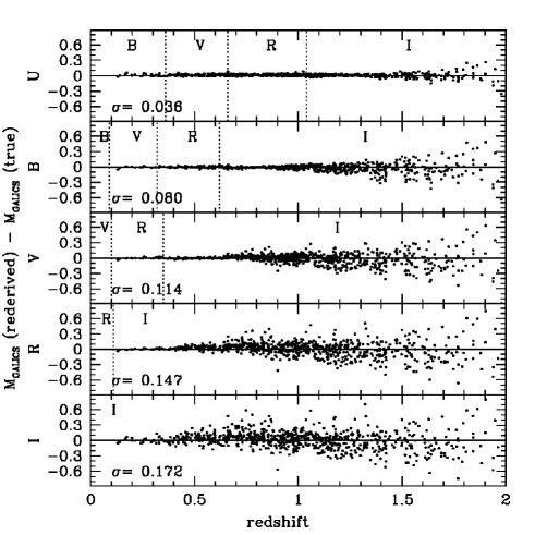
Figure 13: Difference between our ‘rederived’ absolute magnitudes and ‘true’ absolute magnitudes from GALICS as a function of redshift, in the $U$, $B$, $V$, $R$ and $I$ reference bands from the top to the bottom panels, respectively. The vertical lines indicate the change of $Obs$ filter and the adopted $Obs$ filter is labeled in the corresponding redshift range.

The k-correction depends on the galaxy spectral energy distribution (SED). At high redshift, it is the main source of error and systematic in the absolute magnitude measurement. Using Le Phare, we adjust the best SED template on $U$, $B$, $V$, $R$ and $I$ apparent magnitudes to derive k-corrections. We use a set of templates generated with the galaxy evolution model PEGASE.2 (Fioc & Rocca-Volmerange 1997 ). The templates are computed for eight spectral classes including elliptical, spiral, irregular and starburst, with the initial mass function (IMF) from Rana & Basu (1992), with ages varying between 10 Myr and 14 Gyr. Dust extinction and metal effects are included, depending on the evolution scenario. We derive the absolute magnitude in the reference band $Ref$ from the apparent magnitude in the band $Obs$:

$$M^{Ref}=m^{Obs}-DM(z,H_{0},\Omega_{m},\Omega_{\Lambda})-KC(z,{\rm SED})$$ (1)

with DM the distance modulus and $KC$ defined as follows:

$$KC(z,{\rm SED})=(k^{Ref}(z)+m^{Obs}(z)-m^{Ref}(z))^{{\rm SED}}$$ (2)

with $k^{Ref}$ the k-correction in the reference band (Oke & Sandage 1968 ). To limit the template dependency, the $Obs$ band is chosen automatically to be the closest as possible to the $Ref$ band redshifted in the observer frame. We do not correct the absolute magnitudes for the internal dust extinction related to the considered galaxies.

To check the robustness of our absolute magnitude estimate, we use the GALICS simulations (Hatton et al. 2003 ). We extract a simulated catalogue with $B$, $V$, $R$, $I$ apparent magnitudes and redshifts from the GALICS/MOMAF database. We apply exactly the method described before, to rederive the absolute magnitudes. Fig.13 shows the difference between our measurements and the ‘true’ absolute magnitudes from GALICS. When our procedure to limit the template dependency is efficient, the dispersion remains very small in comparison to the photometric errors. For instance, $\sigma\sim 0.03-0.04$ in the U-band, and we limit the template dependency up to $z=2$. If our procedure can not be applied (since NIR data are not considered here), the dispersion increases. For instance, in the $I$-band the dispersion due to the k-correction is $\sim 0.2$.

A.2 Luminosity function estimators

We describe in this subsection the four standard estimators implemented in ALF, the 1/V_max, C⁺, SWML and STY estimators.

A.2.1 The 1/V_max estimator

The 1/V_max LF estimator (Schmidt 1968 ) is the most often used to derive the LF, because of its simplicity. This estimator requires no assumption on the luminosity distribution. The 1/V_max gives directly the normalization of the LF, assuming implicitly an uniform spatial distribution of the galaxies.

We consider a sample selected between bright and faint apparent magnitude limits, $m_{b}$ and $m_{f}$ respectively. The maximum observable comoving volume in which galaxy $i$ can be detected is given by

$$V_{obs,i}=\int_{\omega}\int^{z_{max,i}}_{z_{min,i}}\frac{d^{2}V}{d\omega dz}d\omega dz,$$ (3)

where $\omega$ is the effective solid angle of the survey, and $V$ is the comoving volume. $z_{min,i}$ and $z_{max,i}$ are the lower and upper redshift limits within a galaxy $i$ can be included in the sample. The LF, $\phi(M)$, is discretized in absolute magnitudes

$$\phi(M)=\sum^{N_{bin}}_{k=1}\phi_{k}W(M_{k}-M),$$ (4)

where the window function $W$ is defined as,

$$W(x)=\left\{\begin{array}[]{rl}1&\mbox{if $-dM/2\leq x<dM/2$}\\ 0&\mbox{otherwise.}\end{array}\right.$$ (5)

$\phi_{k}$ is derived in each absolute magnitude bin $k$ as follows:

$$\phi_{k}dM=\sum^{N_{g}}_{i=1}\frac{w_{i}}{V_{obs,i}}W(M_{k}-M_{i}),$$ (6)

where $N_{g}$ is the number of galaxies of the sample and $w_{i}$ is the weight applied to correct the unidentified sources in the field (see Section 3). We associate the Poisson errors to the 1/V_max following (Marshall 1985 ):

$$\sigma_{\phi_{k}}=\sqrt{\sum_{i=1}^{N_{g}}W(M_{k}-M_{i})\frac{w_{i}^{2}}{{V_{{obs}_{i}}}^{2}}}.$$ (7)

A.2.2 The C⁺ estimator

Lynden-Bell (1971) derived the non-parametric C^- method to overcome the assumption of a uniform galaxy distribution. We use a modified version of the C^-, called C⁺ (Zucca et al. 1997 ). This method is based on the equality:

$$\frac{d\psi}{\psi}=\frac{dX}{C^{+}},$$ (8)

with $\psi$ the cumulative luminosity function, $d\psi$ the variation of the cumulative luminosity function between $M$ and $M+dM$. $dX$ is the number of observed galaxies between $M$ and $M+dM$ and $C^{+}$ is the number of galaxies brighter than $M+dM$ with a redshift lower than the maximum redshift observable. We use a sample sorted from the faintest to the brightest absolute magnitude. We note $C^{+}_{i}$ the value of $C^{+}$ for a galaxy $i$. We introduce the weight $w_{i}$ in $C^{+}_{i}$ as follows:

$$C^{+}_{i}=\sum^{N_{g}}_{j=i,z_{j}\leq z_{max,i}}w_{j}.$$ (9)

We note $f_{i}$ the variation of the cumulative luminosity function in the neighborhood of the galaxy $i$, between $M_{i}^{-}$ and $M_{i}^{+}$. We can write the cumulative luminosity function:

$$\psi(M_{i})=\psi_{i}=\sum^{N_{g}}_{j=i}f_{j}=\psi_{0}-\sum_{j=1}^{i-1}f_{j}.$$ (10)

We impose the limit values $f_{0}=0$ and $\psi_{0}=1$ to normalize the cumulative luminosity function. We obtain the recurrence relation, used to derive the contribution of all galaxies in the sample:

$$f_{i}=\frac{\psi_{i}}{C^{+}_{i}}=\frac{1-\sum_{j=1}^{i-1}f_{j}}{C^{+}_{i}}.$$ (11)

The LF is given by rebinning the contributions $f_{i}$:

$$\phi_{k}dM=\sum_{i=1}^{N_{g}}f_{i}w_{i}W(M_{k}-M_{i}).$$ (12)

Poisson errors are associated as done for the 1/V_max estimator (Eq. 7).

A.2.3 The STY and SWML estimators

The STY (Sandage et al. 1979 ) and the SWML (Efstathiou et al. 1988 , hereafter EEP88) estimators are both derived from maximum likelihood method. The likelihood $\mathcal{L}$ is the joint probability of observing the galaxy sample, taking into account the observational selection effects. The principle of the SWML and STY is to maximize $\mathcal{L}$ with respect to the LF. $\mathcal{L}$ is given by:

$$\mathcal{L}=\prod^{N_{g}}_{i=1}p(M_{i},z_{i})^{\frac{w_{i}}{<w>}}=\prod^{N_{g}}_{i=1}\left(\frac{\phi(M_{i})}{\int^{M_{f,i}}_{M_{b,i}}\phi(M)dM}\right)^{\frac{w_{i}}{<w>}}$$ (13)

where $M_{f,i}$ and $M_{b,i}$ are the faint and bright observable absolute magnitudes of a galaxy $i$ at redshift $z_{i}$. The weight is introduced in $\mathcal{L}$ following Zucca et al. (1994). This weight artificially decreases the size of the error contours derived from the analysis of $\mathcal{L}$, then we balance this weight by the average weight $<w>$. The average weight $<w>$ does not affect the minimization of $\mathcal{L}$.

The STY assumes a functional form for the luminosity distribution. We use the empirical Schechter function (Schechter 1976 ):

$$\phi(L)dL=\phi^{*}e^{-\frac{L}{L^{*}}}\left(\frac{L}{L^{*}}\right)^{\alpha}d\left(\frac{L}{L^{*}}\right).$$ (14)

The likelihood (eq.13) can be written as:

$$\begin{array}[]{lll}ln\mathcal{L}&=&\frac{1}{<w>}[\alpha\sum^{N_{g}}_{i=1}w_{i}lnL_{i}-\\ &&(1/L^{*})\sum^{N_{g}}_{i=1}w_{i}L_{i}-(\alpha+1)lnL^{*}\sum^{N_{g}}_{i=1}w_{i}\\ &&-\sum^{N_{g}}_{i=1}w_{i}ln(\Gamma(\alpha+1,\frac{L_{b,i}}{L^{*}})-\Gamma(\alpha+1,\frac{L_{f,i}}{L^{*}}))]\end{array}$$ (15)

with $\Gamma$ the incomplete Euler gamma function. We use the MINUIT package of the CERN library (James & Roos 1995 ) to minimize $-2ln\mathcal{L}$ (MIGRAD procedure), to obtain the non-parabolic error for each parameter (MINOS procedure) and the error contour $\alpha-M^{*}$ (MNCONT procedure). The crosses of the likelihood surface with $ln\mathcal{L}_{max}-\Delta ln\mathcal{L}$ is used to compute the errors. The threshold $\Delta ln\mathcal{L}$ is chosen in a standard way that depends on the desired confidence level in the estimate ( e.g., $2\Delta ln\mathcal{L}=2.3$ and $2\Delta ln\mathcal{L}=4.61$ to estimate the $\alpha-M^{*}$ error contours with 68% and 90% confidence level ; $2\Delta ln\mathcal{L}=1$ to estimate the one sigma error for one parameter).

The SWML does not assume any functional form for the luminosity distribution. The LF is discretized in absolute magnitude bins like the 1/V_max (see Eq. 4). We maximize $ln\mathcal{L}$ with respect to $\phi_{k}$ to obtain the recurrence equation:

$$\phi_{j}dM=\frac{\sum^{N_{g}}_{i=1}w_{i}W(M_{i}-M_{j})}{\sum^{N_{g}}_{i=1}\frac{w_{i}H(M_{b,i}-M_{j})H(M_{j}-M_{f,i})}{\sum^{N_{bin}}_{k=1}\phi_{k}dMH(M_{b,i}-M_{k})H(M_{k}-M_{f,i})}}.$$ (16)

with

$$H(x)=\left\{\begin{array}[]{rl}0&\mbox{if $x\leq-dM/2$}\\ x/dM+1/2&\mbox{if $-dM/2\leq x\leq dM/2$}\\ 1&\mbox{otherwise.}\end{array}\right.$$ (17)

We add a constraint $g$ on $\phi_{k}$ and rewrite the likelihood as $ln\mathcal{L}^{\prime}=ln\mathcal{L}+\lambda g$ where $\lambda$ is a Lagrangian multiplier. Following EEP88, we choose $g=\sum^{N_{bin}}_{k=1}\phi_{k}dM(L_{k}/L_{f})^{\beta}-1$ with $L_{f}$ the fiducial luminosity and $\beta$ a constant. The error bars are derived from the covariance matrix, denoted $C$, defined as the inverse of the information matrix $I$:

$$C(\phi_{k})=I^{-1}(\phi_{k})=-\left(\begin{array}[]{cc}\frac{\delta^{2}ln\mathcal{L}}{\delta\phi_{i}\delta\phi_{j}}+\frac{\delta g}{\delta\phi_{i}}\frac{\delta g}{\delta\phi_{j}}&\frac{\delta g}{\delta\phi_{j}}\\ \frac{\delta g}{\delta\phi_{i}}&0\end{array}\right)_{\phi_{k}}^{-1}.$$ (18)

The second derivative of the likelihood is given by:

$$\begin{array}[]{lcl}\frac{\delta^{2}ln\mathcal{L}}{\delta\phi_{i}\delta\phi_{j}}&=&-\frac{1}{<w>}\sum^{N_{g}}_{l=1}\frac{w_{l}\delta_{ij}W(M_{l}-M_{j})dM^{2}}{(\phi_{j}dM/(g+1))^{2}}+\\ &&\frac{1}{<w>}\sum^{N_{g}}_{l=1}\frac{w_{l}dM^{2}H1}{(\sum^{N_{bin}}_{k=1}\phi_{k}dMH2/(g+1))^{2}}\end{array}$$ (19)

with $H1=H(M_{b,l}-M_{i})H(M_{i}-M_{f,l})H(M_{b,l}-M_{j})H(M_{j}-M_{f,l})$ and $H2=H(M_{b,l}-M_{k})H(M_{k}-M_{f,l})$. The error bars of the LF (for a normalization given by the constraint) are given by the square root of the diagonal values of the covariance matrix.

A.2.4 Luminosity function normalization

The estimators independent of the spatial density distribution (SWML, STY and C⁺) lose their normalization while the normalization is directly done for the 1/V_max estimator. We adopt the EEP88 density estimator to recover their normalization. The density $n$ is simply the sum over all the galaxy sample of the inverse of the selection function:

$$n=\frac{1}{V_{total}}\sum_{i=1}^{N_{g}}w_{i}\frac{\int^{\infty}_{-\infty}\phi(M)dM}{\int^{M_{f,i}}_{M_{b,i}}\phi(M)dM}.$$ (20)

The comparison with the 1/V_max normalization is a direct and independent check of the LF normalization. The parameter $\phi^{*}$ is directly related to the density $\phi^{*}\int^{\infty}_{-\infty}\phi(M)dM=n$. $\phi^{*}$ is a function of $\alpha$ and $M^{*}$. To estimate the error on $\phi^{*}$, we derive $\phi^{*}$ for the extreme values of the $\alpha-M^{*}$ error contour at one sigma confidence level. We adopt Poisson errors when larger.

References

- (1) Arnouts S., Vandame B., Benoist C. et al., 2001, A&A, 379, 740
- (2) Arnouts S., Moscardini L., Vanzella E. et al., 2002, MNRAS, 329, 355
- Arnouts et al. (2005) Arnouts S., Schiminovich D., Ilbert O. et al., 2005, ApJL, 619L, 43
- (4) Blanton M.R., Hogg D.W., Bahcall N.A. et al., 2003, ApJ, 592, 819
- (5) Bolzonella M. et al., 2005, in preparation
- (6) Bottini D., Garilli B., Maccagni D. et al., 2005, PASP, in press, astro-ph/0409252
- (7) Cimatti A., Mignoli M., Daddi E. et al., 2002, A&A, 392, 395
- (8) de Lapparent V., Galaz G., Bardelli S., Arnouts S., 2003, A&A, 404, 831
- (9) Efstathiou G., Ellis R.S., Peterson B.A., 1988, MNRAS, 232, 431 (EEP88)
- (10) Fioc M. & Rocca-Volmerange B., 1997, A&A, 326, 950
- (11) Fukugita M., Ichikawa T., Gunn J.E. et al., 1996, ApJ, 111, 1748
- (12) Gabasch A., Bender R., Seitz S. et al., 2004, A&A, 421, 41
- (13) Hatton S., Devriendt J.E.G., Ninin S. et al., 2003, MNRAS, 343, 75
- (14) Ilbert O., Tresse L., Arnouts S. et al., 2004, MNRAS, 351, 541
- (15) Ilbert O. et al., 2005, in preparation
- (16) Iovino A. et al., 2005, in preparation
- (17) James F. & Roos M., 1995, MINUIT Function Minimization and Error Analysis, Version 95.03, CERN Program Library D506
- (18) Kron R.G., 1980, ApJS, 43, 305
- (19) Le Fèvre O., Mellier Y., McCracken H. et al., 2004a, A&A, 417, 839
- (20) Le Fèvre O., Vettolani G., Paltani S. et al., 2004b, A&A, 428, 1043
- (21) Le Fèvre O., Vettolani G., Garilli B. et al., 2005, A&A, in press, astro-ph/0409133
- (22) Lilly S.J., Tresse L., Hammer F., Crampton D., Le Fèvre O., 1995, ApJ, 455, 108
- (23) Lin H., Yee H.K.C., Carlberg R.G. et al., 1999, ApJ, 518, 533
- (24) Lynden-Bell D., 1971, MNRAS, 155, 95
- (25) Marshall H.L., 1985, ApJ, 299, 109
- (26) McCracken H.J., Radovich M., Bertin E. et al., 2003, A&A, 410, 17
- (27) Norberg P., Cole S., Baugh C.M. et al., 2002, MNRAS, 336, 907
- (28) Oke J.B. & Sandage A., 1968, ApJ, 154, 21
- (29) Poli F., Giallongo E., Fontana A. et al., 2003, ApJ, 593, L1
- Pozzetti et al. (2003) Pozzetti L., Cimatti A., Zamorani G. et al., 2003, A&A, 402, 837
- (31) Radovich M., Arnaboldi M., Ripepi V. et al., 2004, A&A, 417, 51
- Rana & Basu (1992) Rana N.C. & Basu S., 1992, A&A, 265, 499
- (33) Sandage A., Tammann G.A., Yahil A., 1979, ApJ, 232, 352
- (34) Schechter P., 1976, ApJ, 203, 297
- (35) Schmidt M., 1968, ApJ, 151, 393
- (36) Scodeggio M., Franzetti P., Garilli B. et al., 2005, PASP, submitted, astro-ph/0409248
- (37) Steidel C.C., Adelberger K.L., Giavalisco M., Dickinson M., Pettini M., 1999, ApJ, 519, 1
- (38) Tresse L. et al., 2005, in preparation
- (39) Wolf C., Meisenheimer K., Rix H.-W. et al., 2003, A&A, 401, 73
- (40) Wolf C., Meisenheimer K., Rix H.-W. et al., 2004, A&A, 421, 913
- Zucca et al. (1994) Zucca E., Pozzetti L. & Zamorani G., 1994, MNRAS, 269, 953
- (42) Zucca E., Zamorani G., Vettolani G. et al., 1997, A&A, 326, 477
- (43) Zucca E. et al., 2005, in preparation