The VIMOS VLT Deep Survey

This paper presents the “First Epoch” sample from the VIMOS VLT Deep Survey (VVDS). The VVDS goals, observations, data reduction with the VIPGI pipeline and redshift measurement scheme with KBRED are discussed. Data have been obtained with the VIsible Multi Object Spectrograph (VIMOS) on the ESO-VLT UT3, allowing us to observe $\simeq 600$ slits simultaneously at a spectral resolution $R\simeq 230$. A total of 11564 objects have been observed in the VVDS-02h and VVDS-CDFS “Deep” fields over a total area of $0.61$deg², selected solely on the basis of apparent magnitude $17.5\leq I_{AB}\leq 24$. The VVDS efficiently covers the redshift range $0<z\leq 5$. It is successfully going through the “redshift desert” $1.5<z<2.2$, while the range $2.2<z<2.7$ remains of difficult access because of the VVDS wavelength coverage. A total of 9677 galaxies have a redshift measurement, 836 objects are stars, 90 objects are AGN, and a redshift could not be measured for 961 objects. There are 1065 galaxies with a measured redshift $z\geq 1.4$. When considering only the primary spectroscopic targets, the survey reaches a redshift measurement completeness of 78% overall (93% including less reliable flag 1 objects), with a spatial sampling of the population of galaxies of $\sim 25$% and $\sim 30$% in the VVDS-02h and VVDS-CDFS respectively. The redshift accuracy measured from repeated observations with VIMOS and comparison to other surveys is $\sim$276km/s.

From this sample we are able to present for the first time the redshift distribution of a magnitude-limited spectroscopic sample down to $I_{AB}=24$. The redshift distribution N(z) has a median of $z=0.62$, $z=0.65$, $z=0.70$, and $z=0.76$, for magnitude-limited samples with $I_{AB}\leq 22.5$, $23.0$, $23.5$ and $24.0$ respectively. A high redshift tail above redshift 2 and up to redshift 5 becomes readily apparent for $I_{AB}>23.5$, probing the bright star-forming population of galaxies. This sample provides an unprecedented dataset to study galaxy evolution over $\sim 90$% of the life of the universe.

1 Introduction

Understanding how galaxies and large scale structures formed and evolved is one of the major goals of modern cosmology. In order to identify the relative contributions of the various physical processes at play and the associated timescales, a comprehensive picture of the evolutionary properties of galaxies and AGN, and their distribution in space, is needed over a large volume and a large cosmic time base.

Samples of high redshift galaxies known today reach several hundred to a few thousand objects in the redshift range $0.5-4$, and statistical analysis suffers from small number statistics, small explored volumes and different selection biases for each sample, which prevent detailed analysis. In contrast, in the local universe, large surveys like the 2dFGRS (Colless et al., (2001)) and the Sloan SDSS (Abazajian et al., (2003)) contain from 250000 up to one million galaxies and reach a high level of accuracy in measuring the fundamental parameters of the galaxy and AGN populations. In a similar way, we need to gather large numbers of galaxies at high redshifts to accurately quantify the normal galaxy population through the measurement of e.g. the luminosity function, correlation function and star formation rate, for different galaxy types and in environments ranging from low density to dense cluster cores.

We are currently conducting the VIRMOS VLT Deep Survey (VVDS), a coherent approach to study the evolution of galaxies, large scale structures and AGN. The observational goals are: (1) a “wide” survey: $\sim 100000$ galaxies and AGN observed at low spectral resolution $R\simeq 230$, in 16 deg², to a limiting magnitude $I_{AB}=22.5$ and reaching redshifts up to $\sim 1.3$; (2) a “deep” survey: $\sim 35000$ galaxies and AGN observed at $R\simeq 230$ in 2 deg² and brighter than $I_{AB}=24$, to map evolution over $0\leq z\leq 5$, or 90% of the age of the universe; (3) an “ultra-deep” survey: $\sim 1000$ galaxies and AGN brighter than $I_{AB}=25$, this will probe deep into the luminosity function (3 magnitudes below M* at z=1). In addition, we intend to conduct a selected high redshift cluster survey following up the clusters identified in the “wide” and “deep” surveys, and a high spectral resolution survey, $R\sim 2500-5000$, on a sub-sample of 10000 galaxies selected from the “wide” and “deep” surveys. The observing strategy that we have devised allows us to carry out these goals in an optimized and efficient approach.

Guaranteed Time Observations allow completion of $\sim 40$% of the original survey goals. A Large Program is being proposed to the European Southern Observatory to complete the VVDS as originally planned.

We describe here the survey strategy and the status of the observations in the first epoch “Deep” survey. We detail the scientific motivation in Section 2, the survey strategy in Section 3, the “first epoch” observations in Section 4, the pipeline processing of the VIMOS data with VIPGI in Section 5, the methods followed to measure redshifts in Section 6 and the “first epoch” VVDS-Deep sample in section 7. After a description of the galaxy population probed by the VVDS-Deep in Section 8, we present the redshift distribution of magnitude-limited samples as deep as $I_{AB}=24$ in Section 9, and we conclude in Section 10.

We have used a Concordance Cosmology with $h=0.7$, $\Omega_{m}=0.3$, and $\Omega_{\Lambda}=0.7$ throughout this paper.

2 Survey goals

2.1 Science background

The current theoretical picture of galaxy formation and evolution and of large scale structure growth in the universe is well advanced. In contrast, while existing observations already provide exciting views on the properties and distribution of high redshift objects (Lilly et al., 1995a , Le Fèvre et al., (1995); Steidel et al., (1996), Steidel et al., (1998); Lilly et al., (1996), Madau et al., (1998); Cimatti et al., (2002); Abraham et al., (2004); Wolf et al., (2003)) the samples remain too small, incomplete, affected by large and sometimes degenerate errors from photometric redshifts measurements, or targeted toward specific populations, making it hazardous to relate the evolution observed in different populations at different epochs, study how evolution depends upon luminosity, type or local environment of the populations, and compare results to theoretical predictions.

The massive efforts conducted by the 2dF and Sloan surveys (see e.g. Colless et al., (2001), http://mso.anu.edu.au/2dFGRS/; and Abazajian et al., (2003), http://www.sdss.org/) have been aimed at mapping the distribution and establish the properties of more than one million galaxies in our local environment up to redshifts $\sim 0.3$. As we get to know better our local universe, deep surveys on volumes comparable to the 2dFGRS or SDSS at look back times spanning a large fraction of the age of the universe are required to give access to the critical time dimension and trace back the history of structure formation on scales from galaxies up to filaments with $\sim 100h^{-1}$ Mpc.

This reasoning forms the basis of the VIRMOS-VLT Deep Survey (VVDS). It is intended to probe the universe at increasingly higher redshifts to establish the evolutionary sequence of galaxies, AGN, clusters and large scale structure, and provide a statistically robust dataset to challenge current and future models, from one single dataset. Unlike all previous surveys at the proposed depth, the VVDS is based on a simple and easy to model selection function: the sample is selected only on the basis of I band magnitude, as faint as $I_{AB}=24$ to cover the largest possible redshift range. Although this produces an obvious bias by selecting increasingly brighter galaxies when going to higher redshifts, this selection criterion allows us to perform a complete census of the galaxy population in a given volume of the universe, above a fixed and well-defined luminosity.

2.2 Science motivation

The VVDS is designed to address the following goals:

(1) Formation and evolution of galaxies: The goals are to study the evolution of the main population of galaxies in the redshift range $0<z<5+$ from a complete census of the population of galaxies. Several indicators of the evolution status of the galaxy population will be computed as a function of redshift and spectral type: counts and colors, N(z,type), luminosity and mass function (including vs. spectral type, local galaxy density), star formation rate from various indicators, spectrophotometric properties, merger rate, etc. These indicators will be combined to establish the evolutionary properties of galaxies with unprecedented statistical accuracy. The multi-wavelength approach (radio at VLA, X-ray with XMM, far-IR with Spitzer, and UV with Galex) on the 0226-04 and CDFS deep fields will allow us to probe galaxy evolution from the signatures of different physical processes. HST imaging is on-going on the extended VVDS-10h field selected for the HST-COSMOS program.

From the main low resolution survey, it will be possible to select a well defined sub-sample of high redshift galaxies to be observed at high spectral resolution to determine the fundamental plane of elliptical galaxies at redshifts greater than 1, and up to $z\sim 2$ for star forming galaxies.

(2) Formation and evolution of large scale structures: The formation and evolution of large-scale structures (LSS) is yet to be explored on scales  50-100Mpc at redshifts $0.5<z<5+$. The goal is here to map the cosmic web structure back to unprecedented epochs. From this, a variety of statistical indicators of galaxy clustering and dynamics can be computed, including 3D galaxy density maps, the 2-point correlation functions $\xi(r)$ and $\xi(r_{p},\pi)$ and their projections $w_{p}(r_{p})$, power spectrum, counts in cells and other higher order statistics. The direct comparison of the observed probability distribution function (PDF) of galaxies with the PDF of dark matter halos predicted in the framework of cosmological models will be used to yield a measurement of the evolution of galaxy biasing. The dependence of clustering evolution on galaxy type and luminosity will be investigated. The data will enable comparison of the 3D galaxy distribution with the mass maps produced by weak-shear. These indicators will be combined to form a coherent picture of LSS evolution from $z\sim 4-5$, which will be compared to current large N-body simulations / semi-analytical model predictions.

(3) Formation and evolution of AGN: While the evolution of the bright AGNs is well constrained by the large SDSS and 2dF AGN surveys out to large redshifts (Boyle et al., (2000)), constraints on fainter AGN are weak. With no a priori selection of the survey targets based e.g. on image compactness or color, the detection of AGNs along with the main population of galaxies is feasible (Schade et al., (1995)). This will allow us to study the evolution of the AGN population, in particular the evolution of the luminosity function of QSOs out to $z\sim 5$, and the evolution of the AGN fraction in the galaxy population with redshift. We will also establish the clustering properties of AGN. The 0226-04 and CDFS deep fields are of particular interest because of the multi-wavelength approach including X-ray, radio and far-IR observations.

(4) Formation and evolution of clusters of galaxies: The known sample of high redshift clusters of galaxies above z=0.5 is still small, and volume-limited samples are difficult to obtain. In the VVDS samples, we expect to identify several dozen clusters (depending on cosmological models), half of them at a redshift above 0.5. We will acquire both large-scale velocity information from MOS spectra, and detailed core mapping from IFU spectroscopy. This will enable us to describe both the dynamical state of the clusters and the spectrophotometric evolution of the galaxy population in clusters. The combination of these data with XMM data and weak shear analysis will be particularly powerful to establish the mass properties. We will aim to derive the evolution of the cluster space density.

These scientific goals have been used to establish the observational strategy described below.

3 Survey Strategy

3.1 VVDS surveys

The science goals require a large number of objects over large, deep volumes. They are all addressed in a consistent way by the following observational strategy: (1) Wide survey: 100000 galaxies and AGN observed in the 4 survey fields to $I_{AB}=22.5$, $R\simeq 230$, the survey will sample $\sim 20$% of the galaxies to this magnitude; exposure times are 3000 sec. (2) Deep survey: 35000 galaxies and AGN observed in the 0226-04 field and CDFS to $I_{AB}=24$, $R\simeq 230$, the survey will sample 25% of the galaxies to this magnitude; exposure times are 16200sec; (3) 1000 galaxies and AGN observed in the 0226-04 field to $I_{AB}=25$, $R\sim 200$; (4) 10000 galaxies in all fields to $I_{AB}=22.5$, R=2500-5000; (5) 50–100 cluster cores in all fields to $I_{AB}=24$, R=1000.

Efficient observations can be carried out with $\sim 500-600$ galaxies observed in one single spectroscopic observation for the “deep” survey and about $350-400$ galaxies in the “wide” survey. The sample is designed to bring down the statistical noise, to measure e.g. the luminosity function $\phi*$, M*, or $\alpha$ parameters, or correlation length $r_{0}(z)$ to better than 10% at any of 7 time steps.

3.2 Multi-wavelength surveys

In addition to the U, BVRI, JK surveys conducted by the VVDS team (Le Fèvre et al., 2004a , McCracken et al (2003), Radovich et al., (2003), Iovino et al., (2005), respectively), multi-wavelength surveys are carried out by the VVDS team or under data exchange agreements with other teams. Some of the VVDS fields have been observed at 1.4 Ghz at the VLA (Bondi et al., (2003)), with XMM (Pierre et al. (2003)), by Galex (Arnouts et al., (2004), Schiminovich et al., (2004)) and are being observed by Spitzer (Lonsdale et al., (2003)).

3.3 The VIMOS instrument

The VIsible Multi-Object Spectrograph is installed on the European Southern Observatory (ESO) Very Large Telescope (VLT), at the Nasmyth focus of the VLT unit telescope 3 “Melipal” (Le Fèvre et al., (2003)). VIMOS is a 4-channel imaging spectrograph, each channel (a “quadrant”) covering $\sim 7\times 8$arcmin² for a total field of view (a “pointing”) of $\sim 218$ arcmin². Each channel is a complete spectrograph with the possibility to insert slit masks $\sim 30\times 30$cm² each at the entrance focal plane, broad band filters or grisms to produce spectra on a $2048\times 4096$ pixels² EEV CCD.

The pixel scale is 0.205 arcsec/pixel, providing excellent sampling of the Paranal mean image quality and Nyquist sampling for a slit 0.5 arcsecond in width. The spectral resolution ranges from $\sim 200$ to $\sim 5000$. Because the instrument field at the Nasmyth focus of the VLT is large ($\simeq 1$m), there is no atmospheric dispersion compensator. This requires us to limit observations to airmasses below 1.7.

In the MOS mode of observations, short “pre-images” are taken ahead of the observing run. These are cross-correlated with the user catalog to match the instrument coordinate system to the astrometric reference of the user catalog. Slit masks are prepared using the VMMPS tool, with an automated optimization of slit numbers and position (see Bottini et al., (2005)).

3.4 VVDS fields

The 4 main fields of the VVDS have been selected at high galactic latitude, and are spread around the celestial equator to allow year round survey observations. Each field is $2\times 2$deg². The imaging is deep enough to select the VIRMOS targets at the survey depth without selection effects (see Section 3.6). We have included the Chandra Deep Field South (CDFS, Giacconi et al., (2002)), which is the target of Chandra, HST, XMM and Spitzer multi-wavelength observations, to complement the work of the GOODS consortium (Giavalisco et al., (2004)).

The fields positions and available optical and near-infrared imaging data are summarized in Table 1.

Table 1: VVDS fields: positions and available optical and near-infrared photometry

$$\begin{array}[]{lllcccccc}\hline\cr\vskip 3.0pt plus 1.0pt minus 1.0pt\cr Field&\alpha_{2000}&\delta_{2000}&b&l&$Survey mode$&$Multi-wavelength data$\\ \vskip 3.0pt plus 1.0pt minus 1.0pt\cr\vskip 3.0pt plus 1.0pt minus 1.0pt\cr 0226-04&02h26m00.0s&-04\deg 30\arcmin 00\arcsec&-58.0&-172.0&Deep&B,V,R,I^{a}\\ VVDS-02h&&&&&&J,K^{b}\\ &&&&&&U^{c}\\ \vskip 3.0pt plus 1.0pt minus 1.0pt\cr\hline\cr\vskip 3.0pt plus 1.0pt minus 1.0pt\cr 1003+01&10h03m00.0s&+01\deg 30\arcmin 00\arcsec&42.6&237.8&Wide&B,V,R,I^{a}\\ &&&&&&J,K^{b}\\ \vskip 3.0pt plus 1.0pt minus 1.0pt\cr\vskip 3.0pt plus 1.0pt minus 1.0pt\cr 1400+05&14h00m00.0s&+05\deg 00\arcmin 00\arcsec&62.5&342.4&Wide&B,V,R,I^{a}\\ &&&&&&J,K^{b}\\ \vskip 3.0pt plus 1.0pt minus 1.0pt\cr\vskip 3.0pt plus 1.0pt minus 1.0pt\cr 2217+00&22h17m50.4s&+00\deg 24\arcmin 00\arcsec&-44.0&63.3&Wide&B,V,R,I^{a}\\ &&&&&&J,K^{b}\\ \vskip 3.0pt plus 1.0pt minus 1.0pt\cr\vskip 3.0pt plus 1.0pt minus 1.0pt\cr CDFS&03h32m28.0s&-27\deg 48\arcmin 30\arcsec&-54.5&223.5&Deep&B,V,R,I^{d}\\ VVDS-CDFS&&&&&&HSTB,V,R,I^{e}\\ \vskip 3.0pt plus 1.0pt minus 1.0pt\cr\hline\cr\end{array}$$

• (Le Fèvre et al., 2004a )

• (Iovino et al., (2005))

• (Radovich et al., (2003))

• (Arnouts et al., (2001))

• (Giavalisco et al., (2004))

3.5 Field coverage: VIMOS pointing layout for the VVDS-Deep

The VVDS “Deep” survey is conducted in the central 1.2deg² area of the VVDS-02h field and in the CDFS. In the VVDS-02h area, we have devised a scheme which allows uniform coverage of a central area of $0.92\times 1.33$deg², with 4 passes of the instrument, i.e. each point on the sky has 4 chances of being selected for spectroscopy, using 66 pointings spaced by (2arcmin,2arcmin) in ($\alpha$,$\delta$) as shown in Figure 1.

The VIMOS multiplex allows measurement of on average $\sim 540$ spectra per pointing at the magnitude $I_{AB}\leq 24$; this pointing strategy therefore enables observation of $\sim 35000$ spectra in the “deep” area.

The pointing layout of the VVDS-Wide survey includes 96 pointings to cover $2\times 2$deg² with a grid of pointings overlapping twice; it will be presented elsewhere (Garilli et al., in preparation).

Figure 1: The planned layout and identification numbers of the VIMOS pointings for the VVDS “Deep” survey in the VVDS-02h. A total of 66 pointings is planned, placed on a grid with (2,2) arcmin spacing in ($\alpha$,$\delta$). This layout allows observation of the central area (cross hatched) 4 times, and edge areas twice (hatched) except for the 4 corners which are observed once (triple hatched). See Table 2 for the list of already observed fields and Figure 12 for the layout of objects already observed.

3.6 I-band magnitude-limited sample

The selection function used to identify targets to be observed spectroscopically has a deep impact on the final content of the survey. We have taken the classical approach of a pure magnitude selection of the sample, without any other color or shape criteria: the VVDS “Deep” survey is limited to $17.5\leq I_{AB}\leq 24$ and the “Wide” survey is limited to $17.5\leq I_{AB}\leq 22.5$. The I band selection is made as a compromise to select the galaxy population from the flux emitted by the “old” stellar content above 4000Å up to $z\sim 1$. At redshifts above z=1, this selection criterion implies that galaxies are selected from the continuum emission below 4000Å, going increasingly towards the UV as redshift increases.

We do not to impose any shape criteria on the sample selection. This is dictated by the main requirement to keep QSOs, compact AGN, or compact galaxies in the sample . The “star-galaxy” separation from most photometry codes is known to be only valid for relatively bright magnitudes, with the locus of stars and galaxies in a “magnitude-shape” diagram overlapping for the faintest magnitudes. Eliminating star-like objects on the basis of the shape of the image profile alone would thus eliminate a significant part of the AGN and compact galaxy population with little control over the parent population or redshift domain which is lost. We can test this a posteriori from our unbiased spectroscopic sample; this will be presented elsewhere.

The magnitude selection sets strong requirements on the photometric catalog necessary as input to select the spectroscopic target list. We have conducted the CFH12k-VVDS imaging survey at CFHT to cover the 4 VVDS fields in B, V, R and I bands (Le Fèvre et al., 2004a ). The depth of the imaging survey is $\sim 1$ magnitude deeper than the spectroscopic survey limit, which ensures that there is no a-priori selection against low surface brightness galaxies (McCracken et al (2003)). The multi-color information is used only after the spectroscopic observations, e.g. to help determine k-corrections (Ilbert et al., (2005)). In addition to the core B,V,R, I photometric data, U band photometry (Radovich et al., (2003)) and J, K’ photometry (Iovino et al., (2005)) have been obtained for part of the fields.

4 First epoch observations: the VVDS-Deep survey in VVDS-0226-04

4.1 Preparation of VIMOS observations: VMMPS and database tools

The preparation of VVDS observations is done from the selected list of pointings. The VVDS database implemented under Oracle is used to extract the list of targets allowed in a given pointing, ensure a secure follow-up of the work on each pointing and in particular to treat the overlapping observations. For each pointing a short R-band image is taken with VIMOS ahead of the spectroscopic observations. Upon loading in the database, this “pre-image” is automatically flat-fielded and the detection algorithm of Sextractor (Bertin and Arnouts, (1996)) is run to identify the brightest $\sim 80$ sources, and a catalog of bright sources is produced with coordinates in the VIMOS CCD coordinate system.

The next steps are conducted with the VMMPS tool to design the slit mask layout (Bottini et al., (2005)). The positions of the sources identified from the “pre-image” are cross-correlated with the deep VVDS source catalog (Le Fèvre et al., 2004a ) to derive the transformation matrix from the ($\alpha,\delta$) sky reference frame of the VVDS catalog to the ($X_{CCD},Y_{CCD}$) VIMOS instrumental coordinate system. After placing two reference apertures on bright stars for each pointing quadrant (see below), slits are then assigned to a maximum number of sources in the photometric catalog. The automated SPOC (Slit Positioning Optimisation Code, see Bottini et al., (2005)) algorithm is run to optimize the number of slits given the geometrical and optical constraints of the VIMOS set-up (Bottini et al., (2005)). We have designed masks with slits of one arcsecond width, and have forced that a minimum of 1.8 arcseconds of sky is left on each side of a targeted object to allow for accurate sky background fitting and removal during later spectroscopic data processing. The typical distribution of slit length in the VVDS is shown in Figure 2. On average, a VVDS-Deep pointing of 4 quadrant masks contains about 540 slits.

Figure 2: Distribution of slit length in 6 of the VVDS-02h pointings.

Upon completion of this step, Aperture Definition files in Pixels (ADP) are produced. ADPs contain the positions, length and width of all slits to be observed, produced using the VIMOS internal transformation matrix from the mask focal plane to the CCD focal plane to transform the coordinates of any VVDS source in the photometric catalog to VIMOS mask coordinates. The ADPs are then sent to the Mask Manufacturing Machine (MMU, Conti et al., (2001)) for the masks to be cut and stored in the VIMOS “mask cabinets” ready for observation. Database handling of objects already targeted ensures no duplication of observations in overlapping areas of adjacent pointings.

4.2 VIMOS observations

We have built Observing Blocks (OBs) using the standard “Jitter” template, with 5 steps along the slit, each separated by 0.7 arcsec, at -1.4, -0.7, 0, 0.7, 1.4 arcsec from the nominal on-target position. Moving the objects along the slit considerably improves the data processing in the presence of the strong fringing produced by the thin EEV CCDs used in VIMOS (see below).

We have been using the LRRED grism together with the RED cutoff filter, which limits the bandpass and order overlap. The useful wavelength range is 5500 to 9400 Å. With one arcsecond slits, the resolution measured at 7500Å is $33$Å, or $R=227$, and the dispersion is $7.14$Å/pixel.

In the “Deep” survey, 10 exposures of 27 minutes each are taken, repeating the shift pattern twice, for a total exposure time of 4.5h. The typical layout of spectra on each CCD of the 4 channels is presented in Figure 3 for the “VVDS-Deep”.

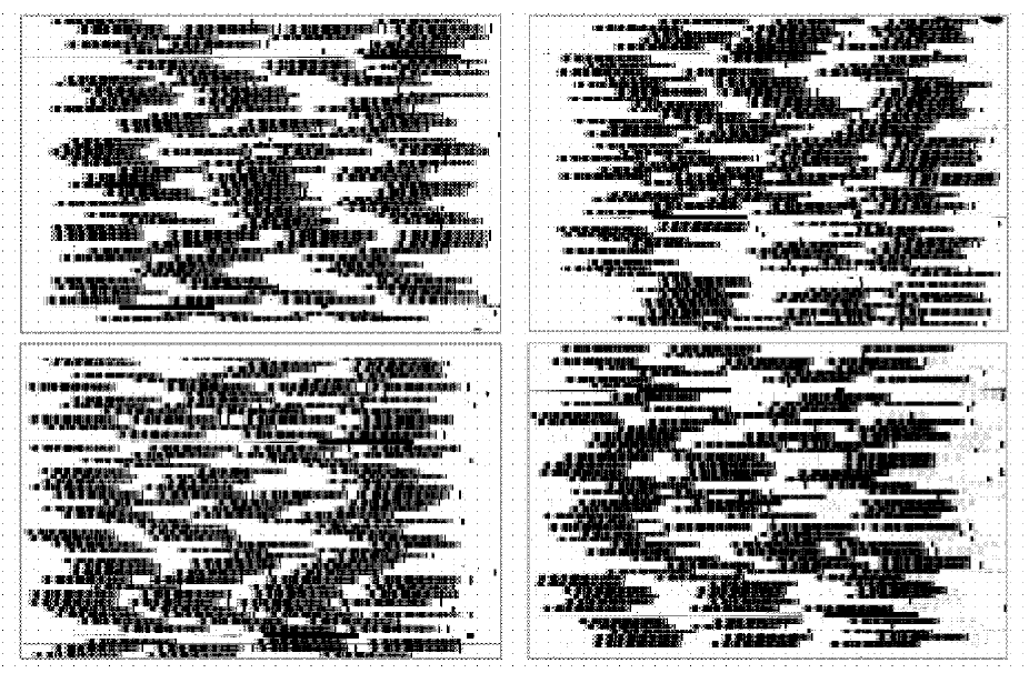
Figure 3: Typical layout of spectra in the 4 quadrants of a VVDS-Wide pointing; more than 550 are observed on average

4.3 Observed fields

The list of “VVDS-Deep” fields observed from October to December 2002 is presented in Table 2. A total of 20 pointings have been observed in the VVDS-Deep area of the VVDS-02h field and 5 pointings in the VVDS-CDFS data (Le Fèvre et al., 2004a ). We have observed $\sim 30$% of the “Deep” area pointings during this period. The first epoch observations of the VVDS-Wide survey will be presented elsewhere (Garilli et al., in preparation).

Table 2: First epoch VVDS-Deep fields observations in the VVDS-02h and VVDS-CDFS

$$\begin{array}[]{lllc}\hline\cr\vskip 3.0pt plus 1.0pt minus 1.0pt\cr$Field$&\alpha_{2000}&\delta_{2000}&$Exposure time (min)$\\ \vskip 3.0pt plus 1.0pt minus 1.0pt\cr\hline\cr\vskip 3.0pt plus 1.0pt minus 1.0pt\cr F02P016&02h25m34.49s&-04\deg 40\arcmin 15.6\arcsec&10\times 27\\ F02P017&02h26m00.83s&-04\deg 40\arcmin 15.6\arcsec&10\times 27\\ F02P018&02h26m27.16s&-04\deg 40\arcmin 15.6\arcsec&10\times 27\\ F02P019&02h26m53.50s&-04\deg 40\arcmin 15.6\arcsec&10\times 27\\ F02P020&02h27m19.83s&-04\deg 40\arcmin 15.6\arcsec&10\times 27\\ F02P027&02h25m34.47s&-04\deg 32\arcmin 37.6\arcsec&13\times 27\\ F02P028&02h26m00.80s&-04\deg 32\arcmin 37.6\arcsec&10\times 27\\ F02P029&02h26m27.13s&-04\deg 32\arcmin 37.6\arcsec&9\times 24+5\times 27\\ F02P030&02h26m53.46s&-04\deg 32\arcmin 37.6\arcsec&10\times 27\\ F02P031&02h27m19.79s&-04\deg 32\arcmin 37.6\arcsec&9\times 27,$except channel 2$,8\times 27\\ F02P038&02h25m34.45s&-04\deg 24\arcmin 59.6\arcsec&11\times 27,$except channel 3, $4\times 27$ (not used)$\\ F02P039&02h26m00.77s&-04\deg 24\arcmin 59.6\arcsec&10\times 27\\ F02P040&02h26m27.10s&-04\deg 24\arcmin 59.6\arcsec&11\times 27\\ F02P041&02h26m53.42s&-04\deg 24\arcmin 59.6\arcsec&10\times 27\\ F02P042&02h27m19.75s&-04\deg 24\arcmin 59.6\arcsec&7\times 27,$except channel 2$,2\times 27$not used$\\ F02P043&02h27m46.07s&-04\deg 24\arcmin 59.6\arcsec&12\times 27\\ F02P050&02h26m00.74s&-04\deg 17\arcmin 21.6\arcsec&10\times 27\\ F02P051&02h26m27.06s&-04\deg 17\arcmin 21.6\arcsec&10\times 27\\ F02P052&02h26m53.39s&-04\deg 17\arcmin 21.6\arcsec&10\times 27,$except channel 2: no data$\\ F02P053&02h27m19.71s&-04\deg 17\arcmin 21.6\arcsec&10\times 27\\ CDFS001&03h32m28.0s&-27\degr 48\arcmin 30\arcsec&10\times 27\\ CDFS002&03h32m37.04s&-27\degr 50\arcmin 30\arcsec&8\times 27\\ CDFS003&03h32m18.95s&-27\degr 50\arcmin 30\arcsec&9\times 27\\ CDFS004&03h32m37.04s&-27\degr 46\arcmin 30\arcsec&12\times 27\\ CDFS005&03h32m18.95s&-27\degr 46\arcmin 30\arcsec&10\times 27\\ \vskip 3.0pt plus 1.0pt minus 1.0pt\cr\hline\cr\end{array}$$

5 Pipeline processing of VIMOS multi-slit data with VIPGI

5.1 VIPGI: the VIMOS Interactive Pipeline Graphical Interface

The pipeline processing of the VVDS data is performed using the VIMOS Interactive Pipeline Graphical Interface (VIPGI, see Scodeggio, et al., (2005) for a full description). This pipeline is built from the same individual C code routines developed by the VIRMOS consortium and delivered to ESO, but was made autonomous so as not to be dependent on the ESO data environment.

5.2 Spectra location

The location of slits is known from the mask design process, hence, knowing the grism zero deviation wavelength and the dispersion curve, the location of spectra is known a priori on the detectors. However, small shifts from predicted positions are possible due to the complete manufacturing and observation process. From the predicted position, the locations of the observed spectra are identified accurately on the 4 detectors and an extraction window is defined for each slit / spectrum.

5.3 Wavelength calibration

The calibration in wavelength is secured by the observation of helium and argon arc lamps through the observed masks. Wavelength calibration spectra are extracted at the same location as the object spectra and calibration lines are identified to derive the pixel to wavelength mapping for each slit. The wavelength to detector pixel transformation is fit using a third order polynomial, resulting in a mean deviation $\sim 1$Å r.m.s. across the wavelength range (Scodeggio, et al., (2005)).

5.4 Sky subtraction, fringing correction

This critical step in the data processing is handled at two levels. First, a low order polynomial (second order) is fit along the slit, representing the sky background contribution at each wavelength position, and subtracted from the 2D spectrum. All exposures of a sequence (5 for the “Wide”, 10 for the “Deep” survey) are then combined with a 3-sigma clipping algorithm. As the object is moved to different positions along the slit following the offset pattern, the median of the 2D sky subtracted spectra produces a frame from which the object is eliminated, but that includes all residuals not corrected by sky subtraction, in particular the fringing pattern varying with position across the slit and wavelength. This sky / fringing residual is then subtracted from each individual 2D sky subtracted frame; these are shifted following the offset pattern to register the object at the same position, and the individual frames are combined with a median, sigma-clipping (usually $2\sigma$), algorithm to produce the final summed, sky subtracted, fringing corrected, 2D spectrum.

5.5 1D wavelength and flux calibrated spectra

The last step done automatically by VIPGI is to extract a 1D spectrum from the summed 2D spectrum, using an optimum extraction following the slit profile measured in each slit (Horne, (1986)). The 1D spectrum is then flux calibrated using the ADU to absolute flux transformation computed from the observations of spectrophotometric standard stars. We have used the star LTT3218 to perform the flux calibration.

A final check of the 1D calibrated spectra is performed and the most discrepant features are removed manually, cleaning each spectrum of e.g. zero order contamination or negative non-physical features.

5.6 Spectrophotometric accuracy

The quality of the spectrophotometry calibration can be estimated by a comparison of integrated magnitudes computed from the flux calibrated spectra, with the broad band photometric measurements coming from the deep imaging data. The comparison shown in Figure 4 is done in absolute terms, comparing the I-band photometric magnitude with the I-band spectroscopic magnitude derived from the integration of the flux of spectra in the equivalent of the I-band photometric bandpass. The spectroscopic I-band magnitude is about 0.2 magnitudes fainter than the photometric magnitude on average, increasing to about 0.5 magnitudes fainter at the bright end of the survey. This can be directly associated with the slit losses inherent to 1 arcsec-wide slits placed on galaxies with sizes larger than the slit width.

The second quality check performed is the comparison of the photometric multi-color magnitudes with the flux in spectra, over the full spectroscopic wavelength range. It is apparent in Figure 5 that the relative spectrophotometry is accurate to $\sim 10$% over the wavelength range $5500-9500$Å.

Figure 4: Difference between the photometric I band magnitude and the I-band magnitude computed from $\sim 1000$ calibrated VVDS spectra. The difference is mainly due to slit losses; no systematic effect in the spectrophotometric calibration is observed vs. magnitude.

Figure 5: Flux-calibrated VVDS spectra compared to the photometry of the VVDS imaging survey after scaling to match to the I band flux (black dots). The spectrophotometric accuracy is conserved over the full wavelength coverage at the 10% level.

5.7 Spectra signal to noise

The signal to noise ratio, measured per spectral resolution element of 1000Å centered on 7500Å, is shown in Figure 6 for the VVDS-Deep. At the faintest magnitudes, the S/N goes down to a mean of $\sim 4$. This S/N is sufficient to enable redshift measurements while at the same time allowing the observation of a large number of objects as shown in Sections 6 and 7.

Figure 6: S/N per spectral resolution element over the magnitude range of the VVDS-Deep survey.

6 Measuring redshifts

6.1 Building up experience over a large redshift base

The VVDS is the first survey to assemble a complete spectroscopic sample of galaxies based on a simple I-band limit down to $I_{AB}=24$, spanning the redshift range $0\leq z\leq\sim 5$. The spectral resolution $R\sim 230$ is adequate to measure redshifts of absorption line galaxies down to the faintest magnitudes observed, as shown in Figure 7. Other examples of spectra are given in Section 7.6.

Magnitude-limited samples have the advantage of a controlled bias in the selection of the target galaxies, which can lead to a secure census of the galaxy population as seen at a given rest-frame wavelength (see e.g. Lilly et al., 1995b ). The drawback is that, as the magnitudes become fainter, the redshift range becomes larger, and identifying redshifts out of a very large range of possibilities becomes increasingly harder from a fixed set of observed wavelengths. The VVDS wavelength range for the VIMOS observations is $5500-9500\AA$. It allows a secure follow-up of the spectral signature of galaxies longward of [OII]3727$\AA$ and minimizes the bias in the identification of galaxy redshifts up to $\sim 1.5$.

A further difficulty in measuring redshifts in the VVDS is that no star/galaxy selection is done a priori before spectroscopy, hence a significant fraction of stars is included in the target list and they have to be identified in the redshift measurement process. Redshift measurements are thus considerably more challenging than in local surveys or for targeted high redshift surveys for which the redshift range is known from an a priori imposed selection function (e.g. Lyman-break galaxies, EROs, Lyman-$\alpha$ emission objects).

In addition, measuring the redshifts of galaxies with $1.5<z<2.7$ is quite challenging within the wavelength domain $5500-9500\AA$ that has generally faint features, and a lack of published observed galaxy templates in the range $1700-3000\AA$ to be used in cross-correlation programs such as the KBRED environments developed for the VVDS (Scaramella et al., in preparation). A dedicated approach had to be followed to ensure sufficient knowledge of rest-frame spectra with VIMOS, especially in the UV between $\sim 1700\AA$ and [OII]3727 where previously observed spectra are not documented in the literature at the S/N level required to be used as reference templates. These templates have been combined with the templates available below $1700\AA$ from the observations of Lyman-break galaxies (Shapley et al., (2003)) to produce templates covering $1100-8000\AA$ rest frame.

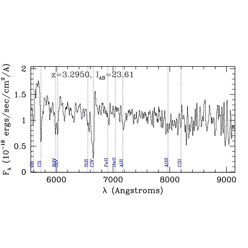
Figure 7: Spectrum of an absorption line galaxy with $I_{AB}=23.61$, and $z=3.2950$, demonstrating the ability of low spectral resolution $R\sim 230$ to measure redshifts from absorption line galaxies down to the very faint end of the survey.

6.2 Crossing the ”redshift desert”

The “redshift desert” has been referred to as the redshift domain between the low–intermediate redshifts measured up to $z\sim 1.3-1.5$ and the high redshift galaxies identified using the Lyman-break technique, with a paucity of galaxies identified at $z\sim 1.5-2.7$. Crossing this “redshift desert” is critical to reduce the incompleteness of deep redshift surveys and to probe the galaxy population at an important time in the evolution.

In a first pass of redshift measurements on the first epoch spectra of the VVDS $I_{AB}=24$ sample (Le Fèvre et al., (2003)), $\sim$10% of galaxy redshifts appeared hard to identify while a significant fraction of these spectra had a good continuum S/N. We have established an iterative approach to identify these objects based on the creation of high S/N rest-frame galaxy templates from observed VVDS spectra, going as far as possible toward the UV and bridging the gap between the well observed wavelength range above [OII]3727$\AA$ and the range below 1700$\AA$ well represented by the templates assembled from $z\sim 3$ Lyman-break galaxies (Shapley et al., (2003)). These new templates have been included in our redshift measurement engine KBRED and tested against the parent samples of galaxies used to produce them, in the range up to redshift $z=1.5$, then up to redshifts $z=2$ and above up to $z\sim 5$ as new redshifts were identified.

This approach has proved successful and has allowed us to identify a large population of objects with $z>1.5$ as shown in Sections 8 and 9. Other groups have also recently efficiently explored this “redshift desert” (Abraham et al., (2004), Steidel et al., (2004)). This “desert” is now demonstrated to be only the result of the selection function imposed by the combination of the faintness of the sources, the wavelength domain of observations, prior lack of observed galaxy templates and the strong OH sky emission features. In effect, the “VVDS redshift desert” is $2.2\leq z\leq 2.7$, mainly associated with the combination of the wavelength domain of spectroscopic observations and the strong OH sky lines.

A complete account of the templates, the methods to identify the galaxies with $z\geq 1.5$, and the remaining incompleteness of the VVDS in the “redshift desert” is given elsewhere (Paltani et al., in preparation).

6.3 Manual vs. automated redshift measurements with KBRED

With templates covering the rest-frame range $1100-8000$Å, two complementary approaches have been followed to measure redshifts: a manual approach and a computer-aided approach with the KBRED automated redshift measuring engine (Scaramella et al., in preparation).

KBRED is a set of routines implemented in the IDL programming environment to perform cross-correlation of observed spectra with reference star and galaxy templates. It includes advanced features to perform Principal Component Analysis of the spectra, projected on a base of reference templates, which are combined to reproduce the spectral energy distribution and measure the best redshift. KBRED can be run automatically on a list of spectra, or manually on a particular spectrum (see Scaramella et al. in preparation, for details).

The first step of redshift measurement has been to run the KBRED routine automatically on all 1D spectra, sky corrected and flux calibrated. This process correctly identifies about 60% of the redshifts, the main difficulty being that, despite intensive testing and code development, it has not been possible to come up with a single objective criterion or set of criteria capable of identifying a posteriori on which spectra KBRED has succeeded or failed to measure a redshift. This is due to the non-linear noise present in the spectra, mostly coming from CCD fringing correction residuals which can be strong above $8000\AA$, making the computation of the classical cross-correlation strength parameter unreliable. Further developments of KBRED are in progress to solve this difficulty.

The second step in redshift measurement is then to visually examine objects one by one in the VIPGI environment, which makes available the 1D and 2D corrected spectra, object profile, sky emission and a set of tools to determine redshifts by hand. The redshift found by the automatic run of KBRED is displayed with the main spectral features expected superimposed on the 1D spectrum. For $\sim 60$% of the spectra the user has simply to quickly verify that the KBRED redshift indeed corresponds to real spectral features and validate the measurement. For the other $\sim 40$% of the spectra, the user notices that KBRED has identified a spectral feature that is noise, as determined upon examination of the 2D spectrum, based on the residuals of the sky subtraction at the location of the strong sky emission OH bands, compounded by the CCD fringing. A visual examination of the spectrum is carried out to mark the secure features, removing the strongest sky-noise features, and either run the VIPGI redshift calculator matching the marked features, or again run KBRED on the cleaned spectrum.

6.4 Checking the redshift measurements

We use teams of data reducers to measure redshifts. For each pointing set of 4 VIMOS quadrants, one person performed the VIPGI processing from raw data to 2D and 1D sky corrected and calibrated spectra. The redshift measurement and quality flag assignment was then performed independently by two persons, and cross-checked together to solve the discrepant measurements. The performance of the team in determining the type of spectra, the spectral features to expect and the instrument signatures (e.g. fringing) increased significantly after the final stage of building a reference set of well-defined templates, as described above. Therefore, a last check of the measurements was performed by a third person, using the latest set of templates, before they were validated and entered in the VVDS database. During this last “super-check” the original value was ultimately changed for about $10$% of the spectra.

Although time consuming, this procedure ensures that minimal machine or personal biases propagate throughout the survey. The redshift measurements and associated quality flags enable a statistical treatment of the overall quality of the survey, as described below.

6.5 Quality flags

We have used a classification of redshift quality similar to the scheme used in the Canada–France Redshift Survey (Le Fèvre et al., (1995)):
– flag 4: a completely secure redshift, obvious spectral features in support of the redshift measurement
– flag 3: a very secure redshift, strong spectral features
– flag 2: a secure redshift measurement, several features in support of measurement
– flag 1: a tentative redshift measurement, weak spectral features including continuum shape
– flag 0: no redshift measurement, no apparent features
– flag 9: one secure single spectral feature in emission, redshift assigned to [OII]3727Å, or $H\alpha$, or in very rare cases to $Ly\alpha$.

A similar classification is used for broad line AGN: when one emission line is identified as “broad” (resolved at the spectral resolution of the VVDS), flags 11, 12, 13, 14, 19 are used to identify the redshift quality. At this stage, no attempt has been made to separate starburst galaxies from type 2, narrow line AGN.

When a second object appears by chance in the slit of the main target, these objects are classified with a “2” added in front of the flag, leading to flags 20, 21, 22, 23, 24, 29. It is important to identify these objects separately from the main sample, as a significant fraction of their flux could be blocked by the slit because it has been centered on the main target, hence reducing the S/N and redshift measurement ability for a given magnitude.

We have classified objects in slits with a clear observational problem as flag=-10, like e.g. objects for which the automated spectra detection algorithm in VIPGI failed, or objects too close to the edge of a slit to allow for a proper sky subtraction. This concerns less than 2% of the slits.

The flag number statistics for the VVDS-Deep sample on the CDFS and VVDS-02h is given in Table 3. The redshift distribution of flag 2 objects reasonably agrees with the overall redshift distribution as shown in Figure 8, but only with a 44% probability that the two populations are drawn from the same sample (as indicated by a KS test), with significant differences between the two populations for $z>1.2$. The redshift distribution of flag 1 objects is significantly different, with a KS test indicating that this population has only a 7% probability of being drawn from the same sample as galaxies with flags 2, 3, and 4. Flag 1 objects are predominantly at $z\geq 1.2$ as shown in Figure 9.

We can estimate the probability of the redshift measurements of being correct for each of the quality flags in two ways. First we have compared the difference in redshift for the 426 objects observed twice in independent observations: we find a concordance in redshift within $dz\leq 0.0025$, of $fc=31\pm 7$% for flags 1, $65\pm 8$% for flags 2, $94\pm 8$% for flags 3, and $99\pm 7$% for flags 4. Assuming that the intrinsic probability of being correct for a given flag is a constant $p_{flag}$, then the fraction of concordant redshifts with the same flag is $p_{flag}^{2}$. From the fraction of concordant redshifts reported above, we therefore find $p_{flag}=fc^{0.5}$, or$p_{flag}=0.55$, $0.81$, $0.97$, $0.995$ for flags 1, 2, 3, and 4, respectively.

A second approach is to compare the spectroscopic redshifts for the whole sample to photometric redshifts derived from the photometric data (Bolzonela et al., in preparation). To obtain a large number of comparisons for galaxies with bright magnitudes $17.5\leq I_{AB}\leq 22$, we have computed photometric redshifts for the full spectroscopic sample from the BVRI photometric data. The $z_{phot}$ vs. $z_{spec}$ comparison in the VVDS-02h field is shown in Figure 10. In addition, to obtain better constraints on photometric redshifts at faint magnitudes $22\leq I_{AB}\leq 24$, we have computed photometric redshifts for the smaller sample for which K photometry is available, as shown in Figure 11. From the brightest objects in Figure 10 and assuming that the flag 4 spectroscopic redshifts are 100% secure, we can identify an intrinsic error of about 5% in the photometric redshift measurements. Removing this fraction of failed photometric redshifts, we deduce that the spectroscopic flag 3 galaxies are $\sim 96$% correct, $\sim 84$% for flag 2, while the “bright” flag 1 would be $\sim 58$% correct. Using the faintest galaxies in Figure 11, we similarly deduce that the faint galaxies with flags 3, 2, and 1 are $\sim 91$%, $\sim 81$%, and $\sim 48$% correct, respectively. We thus determined that objects with quality flags 1, 2, 3, and 4, are $48-58$%, $\sim 81$%, $91-97$% and $\sim 99$% correct, respectively. This is in agreement with the values derived from the repeated spectroscopic observations as reported above.

Table 3: Statistics of redshift quality flags for the First Epoch VVDS-Deep sample

$$\begin{array}[]{lrrrrrrrrrrrrrrrrrrrrrrr}\hline\cr\vskip 3.0pt plus 1.0pt minus 1.0pt\cr$Field$&0&1&2&3&4&9&11&12&13&14&19&20&21&22&23&24&29&211&212&213&214&219&$Total$\\ \vskip 3.0pt plus 1.0pt minus 1.0pt\cr\hline\cr\vskip 3.0pt plus 1.0pt minus 1.0pt\cr$CDFS$&102&140&506&480&285&115&1&6&1&2&0&20&10&34&10&9&1&0&0&0&0&0&1722\\ \leavevmode\nobreak\ \leavevmode\nobreak\ \leavevmode\nobreak\ $galaxies\&QSOs$&-&137&482&458&203&115&1&6&1&2&0&-&10&31&9&5&1&0&0&0&0&0&1461\\ \leavevmode\nobreak\ \leavevmode\nobreak\ \leavevmode\nobreak\ $stars$&-&3&24&22&82&0&-&-&-&-&-&-&0&3&1&4&0&-&-&-&-&-&139\\ $VVDS-02h$&690&1426&2557&2187&2157&304&13&17&27&8&10&149&73&98&54&41&26&0&2&2&0&1&9842\\ \leavevmode\nobreak\ \leavevmode\nobreak\ \leavevmode\nobreak\ $galaxies\&QSOs$&-&1363&2433&2069&1776&304&13&17&27&8&10&-&72&94&52&37&26&0&2&2&0&1&8306\\ \leavevmode\nobreak\ \leavevmode\nobreak\ \leavevmode\nobreak\ $stars$&-&63&124&118&381&0&-&-&-&-&-&-&1&4&2&4&0&-&-&-&-&-&697\\ $Total$&&&&&&&&&&&&&&&&&&&&&&&\\ $VVDS-Deep$&792&1566&3063&2667&2442&419&14&23&28&10&10&169&83&132&64&50&27&0&2&2&0&1&11564\\ $1st epoch$&&&&&&&&&&&&&&&&&&&&&&&\\ \vskip 3.0pt plus 1.0pt minus 1.0pt\cr\hline\cr\end{array}$$

Figure 8: Redshift distribution of flag 2 objects (dashed), compared to the normalized redshift distribution of the flag 3 and 4 objects (open).

Figure 9: Redshift distribution of flag 1 objects (dashed), compared to the normalized redshift distribution of the flag 2, 3 and 4 objects (open).

Figure 10: Comparison of spectroscopic redshifts vs. photometric redshifts computed from BVRI photometry for objects with magnitude $17.5\leq I_{AB}\leq 22.5$, for each of the quality flags 1, 2, 3 and 4 (from bottom left to top right). The fraction of galaxies for which the difference in photometric redshift vs. spectroscopic redshift is less than 0.2 is indicated on the top of each panel. Flags 3 and 4 represent very secure redshift measurements as indicated by the comparison of objects observed spectroscopically twice (see text), hence the dispersion observed for these flags is representative of the error in measuring photometric redshifts. For flags 2 and 1, errors from the photometric redshift estimate and the spectroscopic measurements combine to provide a lower value of 16% and 42% of discrepant redshifts, respectively.

Figure 11: Same as Figure 10 for objects with magnitude $22\leq I_{AB}\leq 24$, for each of the quality flags 1, 2, 3 and 4 (from bottom left to top right), in the VVDS-02h area where K band data is available in addition to BVRI data and makes the photometric redshifts more accurate. The fraction of concordant redshifts is 38%, 72%, 82% and 91% for flags 1, 2, 3 and 4 respectively. Taking into account a photometric redshift failure of $\sim 9$% as shown by the fraction of concordant flag 4 which are known to be $\sim 100$% accurate from spectroscopy, we find that flags 1, 2 and 3 are 47%, 81%, 91% correct, respectively, in this faint magnitude regime where the accuracy of photometric redshifts rapidly decreases.

7 The “First epoch” VVDS-Deep sample

7.1 Galaxies, stars, and QSOs

A total of 10157 galaxies have a spectroscopically measured redshift, 8591 for primary targets with flags $\geq 2$, and an additional 1566 with flag 1. An additional 278 galaxies with flags $\geq 2$ and 83 with flag 1 have been measured as secondary targets appearing by chance in the slit of a primary target.

A total of 836 stars have been spectroscopically measured in the VVDS-02h and the VVDS-CDFS (19 as secondary targets). This was expected since no apriori selection was made against compact objects in the photometric catalog.

There are 71 spectroscopically identified QSOs (flags 12, 13, 14, 19) ranging in redshift from $z=0.172$ to $z=3.863$, and an additional 14 QSOs with flag 11. This unique sample probes the faint end of the AGN luminosity function at high redshift, and will be described extensively in subsequent papers (Gavignaud et al., Zamorani et al., in preparation).

7.2 Spatial distribution of observed galaxies

The spatial distribution of galaxies in the first epoch observations of the VVDS-02h field is shown in Figure 12, for a total sampled area of $1750$arcmin². Together with the VVDS data obtained in a $453$arcmin² area around the CDFS (Le Fèvre et al., 2004b ), a total $2203$arcmin², a $0.61$deg² area has been surveyed. This constitutes an unprecedented spectroscopic survey area at a depth as deep as $I_{AB}=24$.

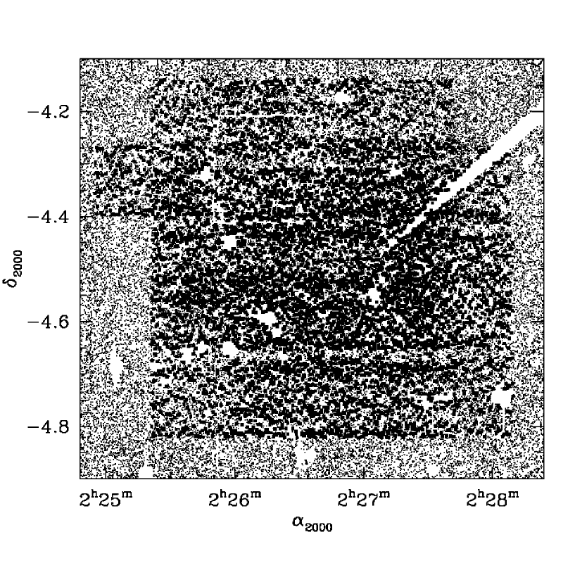
Figure 12: Distribution of galaxies observed in VVDS-02h

7.3 Target sampling rate

The current sampling of the $17.5\leq I_{AB}\leq 24$ photometric sources by the VVDS is indicated in Figure 13 for the VVDS-02h field, while the sampling in the VVDS-CDFS is almost constant at 30% (Le Fèvre et al., 2004b ). Spectra have been obtained in the VVDS-02h for a total of 22.8% of the photometric sources, averaged over the whole area observed, while in the central area corresponding to about two third of the field, $\sim 40$% of the photometric sources have been measured. The slit optimization technique used in VMMPS favors slit placement on smaller objects (Bottini et al., (2005)), hence the ratio of spectroscopically observed objects to objects in the photometric catalog is not constant with magnitude for the VVDS-02h, while this optimization has not been used for the VVDS-CDFS.

Figure 13: Number and fraction of objects observed in the VVDS-02h, compared to the total number of objects in the photometric catalog with $17.5\leq I_{AB}\leq 24$

7.4 Redshift accuracy

The accuracy of the redshift measurements can be estimated from the independent observations of the same objects either within the VVDS or with other instruments. We have observed 160 objects twice in the CDFS fields (Le Fèvre et al., 2004b ), and 266 objects twice in the VVDS-02h. The redshift difference between observations in the CDFS and in the VVDS-02h is plotted in Figure 14; we find that the difference between two measurements has a Gaussian distribution with $\sigma_{z}=13\times 10^{-4}$, or $\sim 390$km/s, hence the accuracy of single redshift measurements is $390/(2)^{0.5}$ or $276$km/s. The 33 galaxies observed in common by VIMOS in the VVDS and FORS2 on the VLT by the GOODS team in the CDFS (Vanzela et al., (2004)) provide an external check of our measuring scheme. As shown in Figure 15, the difference between the two measurements has a $\sigma_{z_{VVDS}-z_{FORS}}=12.6.10^{-4}$, $378$km/s, very similar to what is found from the repeat observations in the VVDS.

Figure 14: Difference in redshift measurements for 266 galaxies observed twice in the VVDS-02h and 139 galaxies observed twice in the VVDS-CDFS. The difference has a Gaussian distribution with $\sigma_{z}=13\times 10^{-4}$ or 390km/s, hence each single redshift measurement has an accuracy $390/(2)^{0.5}$ or $276$km/s

Figure 15: Difference in redshift measurements for 33 objects in common between the VVDS-CDFS sample and the FORS2-GOODS observations of Vanzela et al., (2004). The difference has a mean $dz=8.4.10^{-4}$ and a $\sigma_{z}=12.6.10^{-4}$ or 378km/s

7.5 Completeness vs. magnitude

The completeness in redshift measurement is indicated in Figure 16. Using only the best quality flags (flags 2,3,4,9), the redshift measurement completeness is 78%, while including the less secure flag 1 objects it reaches 93%. The incomplete fraction translates into a sampling of the galaxy population which varies with galaxy type and redshift. This is modeled to compute statistical indicators like the luminosity function (Ilbert et al., (2005)).

Figure 16: Completeness of the $I_{AB}\leq 24$ sample in the VVDS-02h field. (Bottom panel) The magnitude distribution of galaxies with flags 0, 1, 2, 3+4 and 9; (Central panel) The magnitude distribution of galaxies with all flags (open histogram), compared to the distribution of flags 1 and 2 (filled); (Top panel) The ratio of secure redshift measurements with flags 2,3,4,9 and of all measurements (filled). The overall redshift measurement completeness is 78% (flags 2,3,4,9) and redshifts are measured for 93% of the sample (including flags 1).

7.6 Spectra

Examples of spectra in the various redshift ranges are given in Figures 17 to 20.

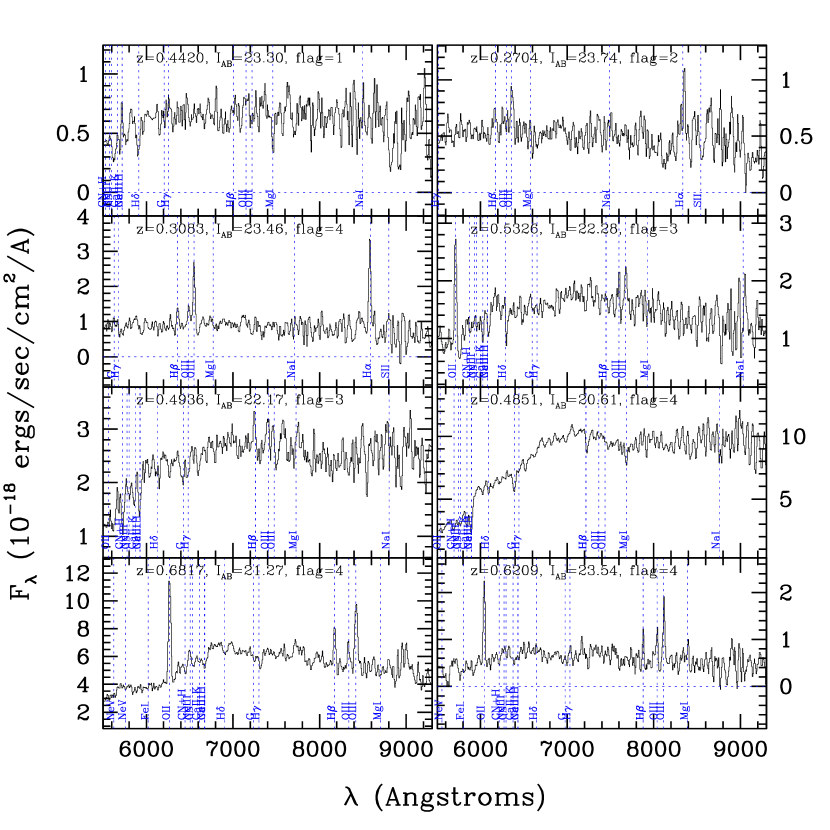
Figure 17: VVDS spectra in the range $0<z\leq 0.7$

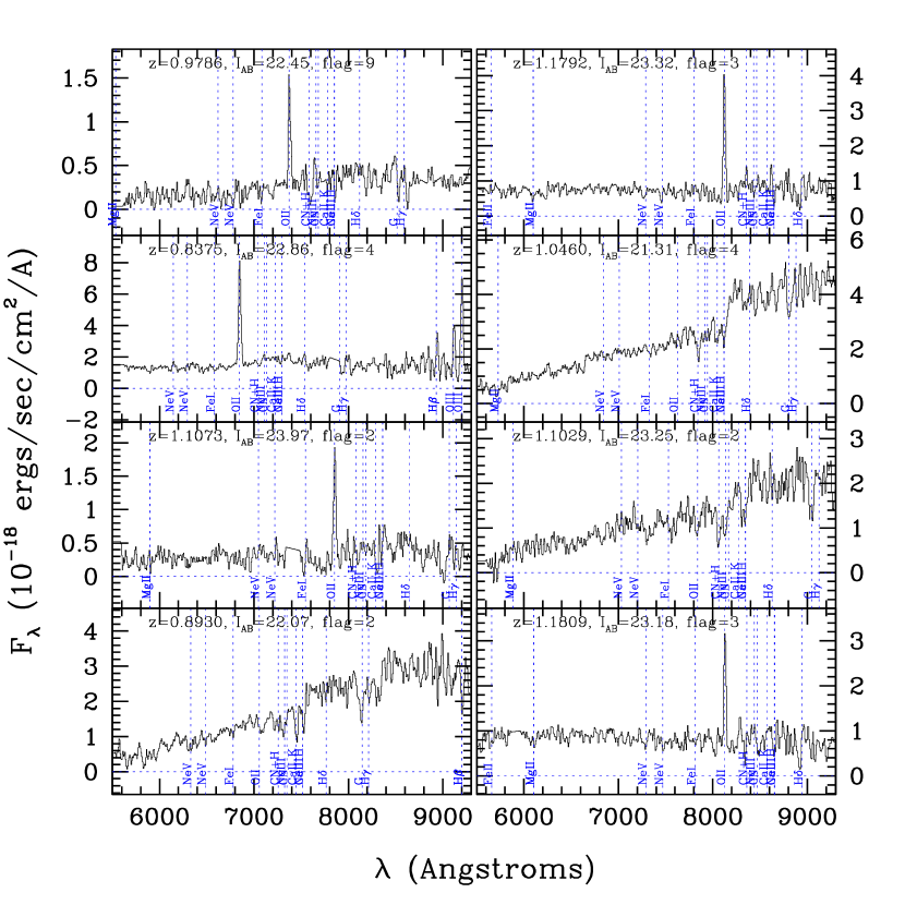
Figure 18: VVDS spectra in the range $0.7<z\leq 1.3$

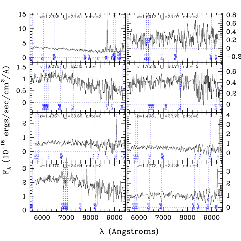
Figure 19: VVDS spectra in the range $1.3<z\leq 2.2$

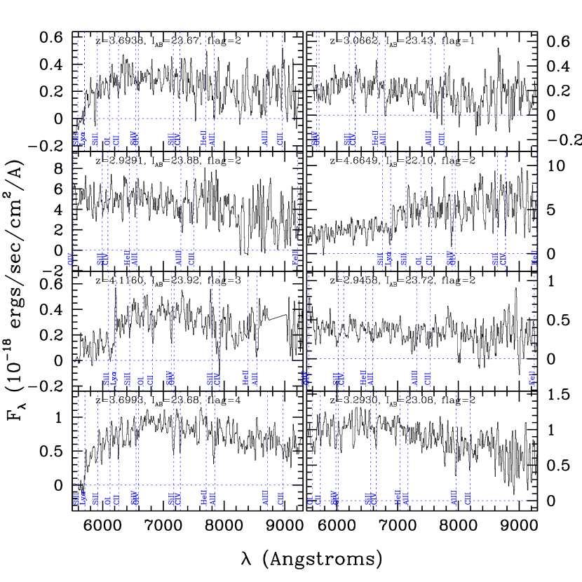
Figure 20: VVDS spectra in the range $2.2<z\leq 5$

8 The galaxy population probed by the VVDS-Deep survey

8.1 Absolute magnitude distribution

The absolute magnitude $M_{B_{AB}}$ distribution vs. redshift is presented in Figure 21. At the lowest redshifts $z<0.4$, the VVDS-Deep observes intrinsically faint galaxies with a mean $M_{B_{AB}}\sim-18$ spanning a large range $-13.5\leq M_{B_{AB}}\leq-21$. At intermediate redshifts $0.4<z<0.8$, galaxies are observed with a mean $M_{B_{AB}}\sim-19.5$ in the range $-17\leq M_{B_{AB}}\leq-22.5$, while for $1<z<2$ observed galaxies are brighter than $M_{B_{AB}}\sim-19$. This is a consequence of the pure apparent I-band magnitude selection, and the shift in the mean and range in absolute luminosity with redshift has to be taken into account when interpreting the observations. As the redshift range is large, the k(z) corrections applied to transform apparent magnitudes to the rest frame B absolute magnitude $M_{B_{AB}}$ work best for redshifts $z<1.5$ for which our broad band photometry can be used to constrain the rest frame B luminosity. At $z>1.5$ the computation of k(z) and $M_{B_{AB}}$ using template fitting becomes more uncertain, and UV rest absolute magnitudes are more appropriate (see Ilbert et al., (2005) for more details).

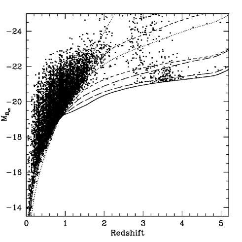
Figure 21: Absolute $M_{B_{AB}}$ magnitude vs. redshift in VVDS-02h. The full sample is shown together with the tracks of CWW templates (Coleman et al., (1980)) and starburst templates used to compute the k(z) correction. At high redshift, the bluest tracks (starburst galaxies) correspond to the faintest absolute $M_{B}$ magnitudes. Each track has been normalized to produce $I_{AB}=24$ at all redshifts. As redshift increases, the computation of k(z) for the rest frame B band becomes increasingly difficult to constrain, hence produces a large range in B-band absolute luminosities for $z\geq 2$. At these high redshifts, and given the wavelength coverage of our spectroscopy and photometry, it is more appropriate to compute absolute magnitudes in the near UV.

8.2 Population at increasing redshifts to $z\sim 5$

The number of galaxies in several redshift slices is given in Table 4. There are:
– 4004 objects with $z\leq 0.75$ and secure redshifts (4528 have measured redshifts when flag 1 objects are included)
– 3344 objects with $0.75<z\leq 1.4$ and secure redshifts (3744 have measured redshifts when flag 1 objects are included)
– 305 objects with $1.4<z\leq 2.5$ and secure redshifts (603 have measured redshifts when flag 1 objects are included)
– 186 objects with $2.5<z\leq 5.0$ and secure redshifts (462 have measured redshifts when flag 1 objects are included)

This constitutes the largest spectroscopic redshift sample over the redshift range $0.4\leq z\leq 5$ assembled to date. A detailed account of the properties of the various populations probed by the VVDS-Deep will be given elsewhere (Paltani et al., in preparation).

Table 4: Number of measured galaxies in redshift slices of the VVDS-Deep First Epoch (primary targets only)

$$\begin{array}[]{lcccccccc}\hline\cr\vskip 3.0pt plus 1.0pt minus 1.0pt\cr$Field$&$0-0.5$&$0.5-0.75$&$0.75-1$&$1-1.4$&$1.4-2.5$&$2.5-3.5$&$3.5-5$&$All z$\\ \vskip 3.0pt plus 1.0pt minus 1.0pt\cr\hline\cr\vskip 3.0pt plus 1.0pt minus 1.0pt\cr$CDFS, flag$\geq 1&280&518&245&265&50&22&15&1395\\ $VVDS-02h, flag$\geq 1&1674&2056&1801&1433&553&264&161&7945\\ \hline\cr$Total$&&&&&&&&\\ $VVDS-Deep$&1954&2574&2046&1698&603&286&176&9340\\ $1st epoch, flag$\geq 1&&&&&&&&\\ \hline\cr$CDFS, flag$\geq 2&259&490&223&243&28&8&7&1258\\ $VVDS-02h, flag$\geq 2&1466&1789&1688&1190&277&101&70&6582\\ \hline\cr$Total$&&&&&&&&\\ $VVDS-Deep$&1725&2279&1911&1433&305&109&77&7840\\ $1st epoch, flag$\geq 2&&&&&&&&\\ \hline\cr\vskip 3.0pt plus 1.0pt minus 1.0pt\cr\hline\cr\end{array}$$

9 Redshift distribution for magnitude-limited samples at $I_{AB}\leq 22.5$ and $I_{AB}\leq 24$

9.1 Redshift distribution for $17.5\leq I_{AB}\leq 22.5$, $17.5\leq I_{AB}\leq 23$, and $17.5\leq I_{AB}\leq 23.5$ magnitude limited samples

From the $17.5\leq I_{AB}\leq 24$ sample, we can extract samples magnitude-limited down to $I_{AB}\leq 22.5$, $I_{AB}\leq 23$, and $I_{AB}\leq 23.5$, which are 93%, 91%, 86% complete respectively including only flags 2,3,4 and 9 (99%, 98%, 96% including objects with flags 1). The redshift distributions shown in Figures 22 to 24 are therefore very secure. The redshift distribution shifts slightly to higher redshifts going from a median redshift of $z=0.62$ for $17.5\leq I_{AB}\leq 22.5$, to $z=0.70$ for $17.5\leq I_{AB}\leq 23.5$. The median redshift and 1st and 3rd quartiles are reported in Table  5. There is only a marginal high redshift tail appearing at $z\geq 2$ in the faintest magnitude bin to $I_{AB}=23.5$. The redshift distribution for a sample down to $I_{AB}\leq 23.5$ does not go down significantly deeper in redshift than a sample limited to $I_{AB}\leq 22.5$, a fact to take into account when planning future redshift surveys.

Figure 22: Redshift distribution for a magnitude-limited sample of 3621 galaxies with $17.5\leq I_{AB}\leq 22.5$, extracted from the sum of the VVDS-CDFS and the VVDS-F02h fields. Galaxies with flags 2,3,4 and 9 are represented by the filled histogram, galaxies with flag 1 by the open histogram. This sample, including flags 2,3,4 and 9, is 93% complete. The median redshift is $z=0.62$ and the mean redshift is $z=0.65$.

Figure 23: Same as Figure 22 for 5124 galaxies with $17.5\leq I_{AB}\leq 23$. This sample, including flags 2,3,4 and 9, is 90% complete. The median redshift is $z=0.67$ and the mean redshift is $z=0.72$.

Figure 24: Same as Figure 22 for 7054 galaxies with $17.5\leq I_{AB}\leq 23.5$. This sample, including flags 2,3,4 and 9, is 85% complete. The median redshift is $z=0.70$ and the mean redshift is $z=0.80$.

9.2 Redshift distribution for $17.5\leq I_{AB}\leq 24$

The redshift distribution of the full First Epoch VVDS-Deep sample is shown in Figure 25. A total of 9340 primary target galaxies is present in this distribution including the VVDS-02h and VVDS-CDFS fields. The sample has a median redshift $z=0.76$, and a significant high redshift tail appears up to $z=5.123$. The $17.5\leq I_{AB}\leq 24$ magnitude selection allows us to continuously sample the galaxy population at all redshifts. The VVDS spectroscopic measurement of the N(z) distribution improves upon previous determinations using photometric redshifts (Brodwin et al., (2005)), in particular in the range $1.4\leq z\leq 5$ where the number of galaxies is small compared to the fraction of catastrophic failures generally encountered when computing photometric redshifts. This fraction of galaxies appearing at all redshifts $2<z<\sim 5$ indicates that the observations are deep enough to probe the brightest part of the population at these redshifts. The gap in the redshift distribution in the interval $2.2\leq z\leq 2.7$ is readily understood in terms of a lower efficiency in measuring redshifts for galaxies in this range because of the VVDS observed wavelength range (see Section 6.2 and Paltani et al., in preparation). Objects with $z>2$ are examined in detail, in particular to evaluate the fraction of flag 1 (and to a much lesser extent, flag 2) galaxies lying at these redshifts; and the properties of this population will be discussed elsewhere (Paltani et al., in preparation).

Table 5: Median redshifts, 1st and 2nd quartiles of the redshift distribution vs. magnitude (primary targets only)

$$\begin{array}[]{lcccc}\hline\cr\vskip 3.0pt plus 1.0pt minus 1.0pt\cr I_{AB}$range$&N_{obj}($flags$\geq 2)&1^{st}$quartile$&$Median$&3^{rd}$quartile$\\ \vskip 3.0pt plus 1.0pt minus 1.0pt\cr\hline\cr\vskip 3.0pt plus 1.0pt minus 1.0pt\cr 18.0-18.5&9&0.13&0.18&0.24\\ 18.5-19.0&23&0.21&0.30&0.37\\ 19.0-19.5&45&0.21&0.30&0.41\\ 19.5-20.0&67&0.24&0.36&0.52\\ 20.0-20.5&111&0.26&0.43&0.64\\ 20.5-21.0&228&0.32&0.50&0.68\\ 21.0-21.5&361&0.38&0.58&0.76\\ 21.5-22.0&569&0.42&0.65&0.89\\ 22.0-22.5&833&0.46&0.70&0.91\\ 22.5-23.0&1156&0.50&0.79&1.11\\ 23.0-23.5&1493&0.56&0.85&1.17\\ 23.5-24.0&1675&0.58&0.90&1.32\\ \vskip 3.0pt plus 1.0pt minus 1.0pt\cr\hline\cr\end{array}$$

Figure 25: Same as Figure 22 for 9141 galaxies with $17.5\leq I_{AB}\leq 24$. This sample, including flags 2,3,4 and 9, is 78% complete. The median redshift is $z=0.76$ and the mean redshift is $z=0.90$.

9.3 Redshift distribution in the VVDS-02h field

The redshift distribution of galaxies in the VVDS-02h field is presented in Figure 26 with smaller redshift bins. The field shows an alternance of strong density peaks and almost empty regions, with strong peaks identified all across the redshift range, although less prominent at $z>\sim 2$. This is the first time that the large-scale structure distribution of galaxies has been probed on transverse scales $\sim 30$h^-1 Mpc at these redshifts. A detailed analysis of the clustering properties of galaxies will be published elsewhere (Le Fèvre et al., (2005), Marinoni et al., (2005)).

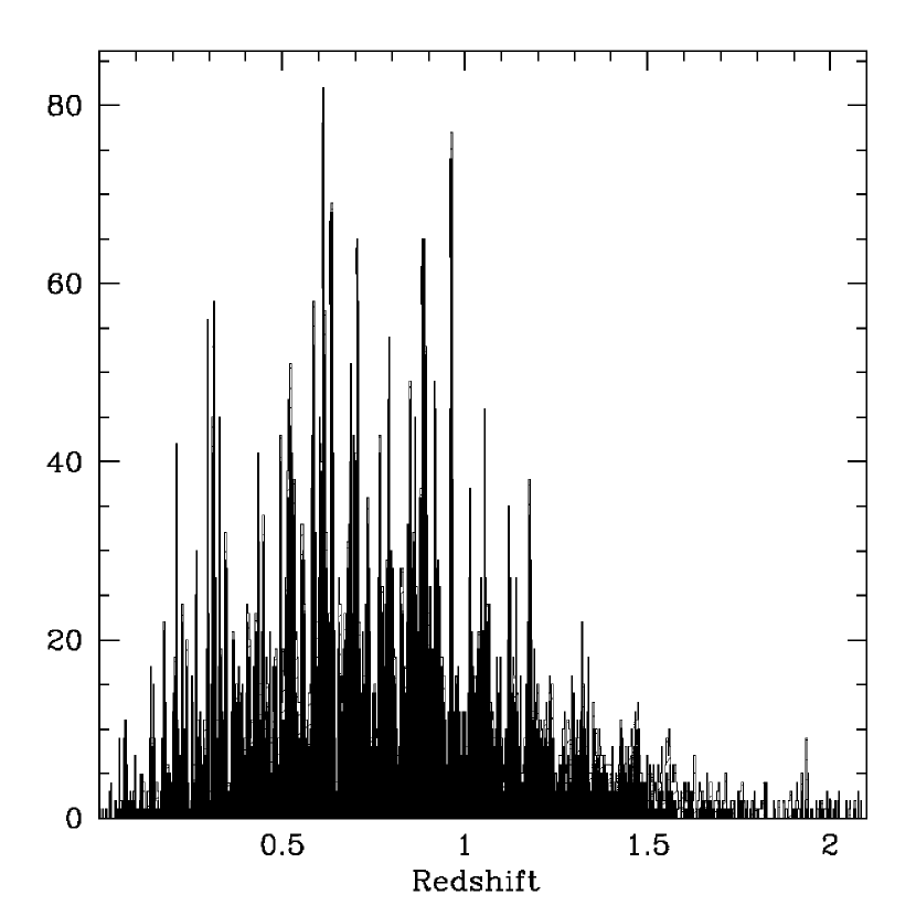
Figure 26: Redshift distribution for galaxies in the VVDS-02h field with $0\leq z\leq 1.7$, for galaxies with redshift quality flags 2,3,4,9 (solid histogram) and galaxies with redshift quality flag 1 (dashed histogram). The redshift bin is dz=0.0033.

10 Conclusion and summary

We have presented the strategy and the first epoch data of the VVDS, an I-band limited deep redshift survey of the distant universe. We have been able to observe 11564 objects in the range $0\leq z\leq 5.2$, in a total area of $\sim 2200$arcmin² in the VVDS-02h and VVDS-CDFS fields, which is thus the largest deep redshift survey at a depth $17.5\leq I_{AB}\leq 24$ to date.

The multi-slit observations with the VLT-VIMOS instrument and heavy data processing with our VIPGI pipeline are described. Emphasis has been placed on the measurement of redshifts using the KBRED automated redshift measuring engine and the associated quality control. Independent redshift measurements have been produced and compared between two survey members, a final check was performed by a third party, and quality flags assigned to each redshift measurement. Repeated observations of the same objects in independent observations have allowed us to quantify the velocity accuracy of the survey as $276$km/s. From these repeated measurements, and using photometric redshifts, we have been able to quantify the reliability of each of the redshift quality flags, and hence to derive the completeness of the survey in terms of the fraction of secure redshift measurements.

A total of 9340 redshifts have been measured on primary targets (7840 objects have the most secure flags 2, 3, 4 and 9), and an additional 342 redshifts were obtained on secondary targets falling in the multi-slits by chance (of which 260 are the most secure). A total of 603 galaxies (305 with the most secure redshifts) have been measured in the range $1.4\leq z\leq 2.5$, and 462 in the range $2.5\leq z\leq 5.2$ (186 with the most secure redshifts). Without a priori compactness selection in the photometric catalog our spectroscopic sample includes 836 galactic stars, but 90 QSOs have been successfully identified. Following the quality flags associated with the redshift measurements, the sample is 78% complete (secure redshifts), while 93% of the sample has a redshift measured. We have presented the core properties of the sample in terms of spatial distribution, absolute magnitude and B-I color vs. redshift, and presented examples of observed spectra, revealing the wide range of galaxy types and luminosities present in the survey.

We also presented the redshift distribution of magnitude limited samples down to $I_{AB}=24$. For samples purely selected in I-band magnitude, with $17.5\leq I_{AB}\leq 22.5$, $17.5\leq I_{AB}\leq 23.0$ and $17.5\leq I_{AB}\leq 23.5$, we find a median redshift of $z=0.62$, $0.67$ and $0.70$, respectively. For the complete first epoch $17.5\leq I_{AB}\leq 24.0$ VVDS-Deep sample, we find that the median redshift is $z=0.76$, with a significant high redshift tail $1.5<z<5.2$ readily apparent.

The first epoch VVDS dataset presented here is used extensively by the VVDS team to measure evolution in the galaxy population, as presented in joint papers and several papers in preparation. It provides an unprecedented sample to study galaxy evolution over 90% of the life of the universe.

References

- Abazajian et al., (2003) Abazajian, K., Adelman-McCarthy, J.K., Agueros, M.A., et al., 2003, A.J., 126, 2081
- Abraham et al., (2004) Abraham, R.G., Glazebrook, K., McCarthy, P.J., Crampton, D., Murowinski, R., Jorgensen, I., et al., AJ, in press (astro-ph/0402436)
- Arnouts et al., (2001) Arnouts, S.; Vandame, B.; Benoist, C.; Groenewegen, M. A. T.; da Costa, L.; Schirmer, M.; Mignani, R. P.; Slijkhuis, R.; Hatziminaoglou, E.; Hook, R., 2001, A&A, 379, 740
- Arnouts et al., (2004) Arnouts, S., Schiminovich, D. , Ilbert, O., et al., 2004, Ap.J., 619, 43
- Bertin and Arnouts, (1996) Bertin, E., Arnouts, S., A&A SUp., 124, 163
- Bondi et al., (2003) Bondi, M., Ciliegi, P., Zamorani, G., Gregorini, L., Vettolani, P., Parma, P., et al., 2003, A&A, 403, 857
- Bottini et al., (2005) Bottini, D., Garilli, B., Maccagni, D., et al., 2005, PASP, in press
- Boyle et al., (2000) Boyle, B.J., Shanks, T., Croom, S.M., Smith, R.J., Miller, L., Loaring, N., Heymans, C., 2000, MNRAS, 317, 1014
- Brodwin et al., (2005) Brodwin, M., Lilly, S.J., Porciani, C., et al., Ap.J., astro-ph/0310038
- Cimatti et al., (2002) Cimatti, A., Daddi, E., Mignoli, M., Pozetti, L., Renzini, A., Zamorani, G., Broadhurst, T., Fontana, A., Saracco, P., Poli, F., et al., 2002, A&A, 381, 68
- Coleman et al., (1980) Coleman, G.D., Wu, C.C., Weedman, D.W., 1980, Ap.J.S., 43, 393
- Colless et al., (2001) Colless, M.M., Dalton, G., Maddox, S., et al., 2001, MNRAS, 328, 1039
- Conti et al., (2001) Conti, G., Mattaini, E., Maccagni, D., Sant’Ambrogio, E., Bottini, D., Garilli, B., Le Fèvre, O., Saïsse, M., Voët, C., et al., 2001, PASP, 113, 452.
- Giacconi et al., (2002) Giacconi, R., Zirm, A., Wang, J., Rosati, P., Nonino, M., Tozzi, P., Gilli, R., Mainieri, V., Hasinger, G., Kewley, L., Bergeron, J., Borgani, S., Gilmozzi, R., Grogin, N., Koekemoer, A., Schreier, E., Zheng, W., Norman, 2002, Ap.J.Supp., 139, 369
- Giavalisco et al., (2004) Giavalisco, M., Dickinson, M., Ferguson, H.C., et al., 2004, Ap.J., 600, L93
- Horne, (1986) Horne, K., 1986, PASP, 98, 609
- Ilbert et al., (2005) Ilbert, O., Tresse, L., Zucca, E., et al., 2005, in press (astro-ph/0409134)
- Iovino et al., (2005) Iovino, A., McCraken, H.J., Garilli, B., et al., A&A, submitted
- Le Fèvre et al., (1995) Le Fèvre, O., Crampton, D., Lilly, S.J., Hammer, F., Tresse, L., 1995, Ap.J., 455, 60
- Le Fèvre et al., (1996) Le Fèvre, O., Hudon, D., Lilly, S.J., Crampton, D., Hammer, F., Tresse, L., 1996, ApJ 461, 534
- Le Fèvre et al., (2003) Le Fèvre, O., Vettolani, G., Maccagni, D., and the VVDS consortium, 2003, The Messenger 111, 18
- Le Fèvre et al., (2003) Le Fèvre, O., Vettolani, G., and the VVDS consortium, 2003, International Astronomical Union Symposium no. 216, held 14-17 July, 2003 in Sydney, Australia, V.216, 183
- (23) Le Fèvre, O., Mellier, Y., McCracken, H.J., Foucaud, S., Gwyn, S., Radovich, M., Dantel-Fort, M., Bertin, E., Moreau, C., Cuillandre, J.C., Pierre, M., Le Brun, V., Mazure, A., Tresse, L., 2004a, A&A, 417, 839
- (24) Le Fèvre, O., Vettolani, G., Paltani, S., et al., 2004b, A&A, 428, 1043
- Le Fèvre et al., (2005) Le Fèvre, O., Guzzo, G., Meneux, B., et al., 2005, A&A, in press (astro-ph/0409136)
- (26) Lilly, S.J., Le Fèvre, O., Crampton, D., Hammer, F., Tresse, L., 1995, Ap.J., 455, 50
- (27) Lilly, S.J., Tresse, L., Hammer, F., Crampton, D., Le Fèvre, O., 1995, ApJ 455, 108
- Lilly et al., (1996) Lilly, S.J., Le Fèvre, O., Hammer, F., Crampton, D., 1996, ApJ, 460, L1
- Lonsdale et al., (2003) Lonsdale, C.J., Smith, H.E., Rowan-Robinson, M., Surace, J., Shupe, D., Xu, C., Oliver, S., Padgett, D., Fang, F., Conrow, T., et al., 2003, PASP, 115, 897
- McCracken et al (2003) McCracken, H.J., Radovich, M., Bertin, E., Mellier, Y., Dantel-Fort, M., Le Fèvre, O., Cuillandre, J.-C., Gwyn, S., Foucaud, S., Zamorani, G., 2003, A&A, 410, 17
- Madau et al., (1998) Madau et al., 1998, ApJ, 498, 106
- Marinoni et al., (2005) Marinoni, C., Le Fèvre, O., Meneux, B., et al., A&A, submitted
- Pierre et al. (2003) Pierre, M., Valtchanov, I., Dos Santos, S., 2004, JCAP, 09, 011
- Radovich et al., (2003) Radovich, M., Arnaboldi, M., Ripepi, V., Massarotti, M., McCracken, H.J., Mellier, Y., Bertin, E., Le Fèvre, O., Zamorani, G., et al., 2004, 417, 51
- Schade et al., (1995) Schade, D., Crampton, D., Hammer, F., Le Fèvre, O., Lilly, S.J., 1995, MNRAS, 278, 95.
- Schiminovich et al., (2004) Schiminovich, D., Ilbert, O., Arnouts, S., et al., 2004, Ap.J., 619, 47
- Scodeggio, et al., (2005) Scodeggio, M., Franzetti, P., Garilli, B., Zanichelli, A., et al., PASP, submitted
- Shapley et al., (2003) Shapley, A.E., Steidel, C.C., Pettini, M., Adelberger, K.L., 2003, ApJ, 588, 65
- Steidel et al., (1996) Steidel, C.C., Giavalisco, M., Pettini, M., Dickinson, M., Adelberger, K.L., 1996, ApJ, 462, L17
- Steidel et al., (1998) Steidel, C.C., Adelberger, K.L., Dickinson, M., et al., 1998, ApJ, 492, 428
- Steidel et al., (2004) Steidel, C.C., Shapley, A.E., Pettini, M.; Adelberger, K.L., Erb, D.K., Reddy, N.A., Hunt, M.P., 2004, ApJ, 604, 534
- Vanzela et al., (2004) Vanzella, E., Cristiani, S., Dickinson, M., Kuntschner, H., Moustakas, L.A., Nonino, M., Rosati, P., Stern, D., Cesarsky, C., Ettori, S., Ferguson, H.C., Fosbury, R.A.E, Giavalisco, M., Haase, J., Renzini, A., Rettura, A., Serra, P., 2005, A&A, 434, 53
- Wolf et al., (2003) Wolf, C., Meisenheimer, K., Rix, H.W., Borch, A., Dye, S., Kleinheinsich, M., 2003, A&A, 401, 73