Compact radio cores: from the first black holes to the last

Abstract

One of the clearest signs of black hole activity is the presence of a compact radio core in the nuclei of galaxies. While in the past the focus had been on the few bright and relativistically beamed sources, new surveys now show that essentially all black holes produce compact radio emission that can be used effectively for large radio surveys. Radio has the advantage of not being affected as much by obscuration. With the Square Kilometer Array (SKA) these cores can be used to study the evolution of black holes throughout the universe and even to detect the very first generation of supermassive black holes. We start by introducing some of the basic properties of compact radio cores and how they scale with accretion power. The relative contribution of jets and radio cores to the Spectral Energy Distribution is strongest in sub-Eddington black holes but also present in the most luminous objects. Radio and X-rays are correlated as a function of black hole mass such that the most massive black holes are most suited for radio detections. We present a radio core luminosity function for the present universe down to the least luminous AGN. The SKA will essentially detect all dormant black holes in the local universe, such as that in our Milky Way, out to several tens of Megaparsecs. It will also be able to see black holes in the making at redshifts $z>10$ for black hole masses larger than $10^{7}M_{\odot}$. Finally, we suggest that the first generation of black holes may have jets that are frustrated in their dense environment and thus appear as Gigahertz-Peaked-Spectrum (GPS) sources. Since their intrinsic size and peak frequency are related and angular size and frequency scale differently with redshift, there is a unique region in parameter space that should be occupied by emerging black holes in the epoch of reionization. This can be well probed by radio-only methods with the SKA.

1 Introduction

Clearly, one of the key issues in cosmology centers on the nature of the very first self-radiating objects in the universe. Undoubtedly among these objects will be the first generation of stars and progenitors of galaxies. However, for some reasons, an almost unavoidable consequence of galaxy and star formation is the formation of black holes (e.g., Ferrarese & Merritt 2000, Gebhardt et al. 2000). Formation processes can be manifold, through collapse of a massive star, through collapse of a star cluster (Portegies Zwart et al. 2004), or through the collapse of inner parts of a galaxy. Accordingly, the masses spanned by astrophysical black holes ranges from stellar ($<10^{2}M_{\odot}$) to intermediate ($10^{2}-10^{4}M_{\odot}$, yet to be confirmed) to supermassive ($10^{4}-10^{10}M_{\odot}$). As formation processes of black holes are poorly understood – we do not even understand supernovae as progenitors to stellar black holes (Buras et al. 2003) – it is very difficult to predict which types of black holes will have formed first, when, and how.

It is quite possible, however, that the first black holes could have played an important role in regulating star formation (e.g., Silk & Rees 1998) or even contributed to the re-ionization of the universe. As discussed elsewhere (Furlanetto & Briggs, this volume) the so-called epoch of reionization, where the neutral remnant gas of the big bang is re-ionized by the first radiating objects, is not well constrained. An early start of reionization as indicated by WMAP polarization measurements (Kogut et al. 2003) may in fact even require the contribution from black holes as discussed in Ricotti & Ostriker (2003) and Ricotti, Ostriker, & Gnedin (2003). Also, the suggestion that $10^{9-10}M_{\odot}$ black holes may have existed at $z>6$ (e.g., Willott, McLure, & Jarvis 2003; Fan et al. 2003) indicates that supermassive black hole formation was rapid and must have preceded or was coeval with the epoch of reionization.

The only way to detect black holes at large distances is through their strong emission, when they light up in the nuclei of galaxies and appear as quasars or active galactic nuclei (AGN). It is therefore important to understand how black holes operate and radiate.

The central engine of AGN is usually thought to consist of the black hole, an accretion inflow, probably accompanied by a hot corona, and a relativistic jet (Shakura & Sunyaev 1973, Sunyaev & Trümper 1979, Mirabel & Rodriguez 1999). The same is true also for black hole X-ray binaries (XRBs) of stellar masses and it indeed appears that both mass scales have a lot in common (see Fender, this volume; Fender & Belloni 2004).

Standard accretion disk theory has successfully explained the ‘big blue bump’ in Quasars or the soft X-ray emission of XRBs in the high state, its emission can usually be described by multi-color black body radiation from the surface of an optically thick disk. The jet on the other hand has an extremely broad spectral energy density (SED). At least for blazars jet emission can be seen from radio up to $\gamma$-rays (see e.g., Montigny et al. 1995). The jet SED has two components, at lower photon energies the emission is thought to be synchrotron emission, while the X-rays and $\gamma$-rays originate from inverse Compton processes (see e.g., Gursky & Schwartz 1977, Fossati et al. 1998). In X-ray binaries and some BL Lacs synchrotron might even contribute to the X-rays (Markoff, Falcke, & Fender 2001) .

Understanding the SED and its dependence on parameters is crucial for identifying the right strategy for deep surveys of black holes throughout the universe, up into and beyond the epoch of reionization.

Both the jet and the disk emission are anisotropic, the jet emission due to relativistic boosting and the disk due to its geometry and possibly an obscuring torus. The orientation dependence was used in the successful unification schemes of AGN (c.f., Antonucci 1993, Urry & Padovani 1995). Besides the inclination of the symmetry axis of the system the main parameters governing its appearance are thought to be the black hole mass and the accretion rate. Additionally the appearance of the central engine may depend on the spin of the black hole and the ambient medium.

Using mass and accretion rate AGN and XRBs can be roughly unified into thermally (high-power, radiatively efficient disks) and non-thermally (low-power, radiatively inefficient) dominated sources, where the non-thermal emission may come entirely from the radio jet in quite a few cases (Falcke, Koerding, & Markoff 2004). This makes it difficult to rely on only one wavelength range to identify AGN activity.

The radio part of the SED, however, seems to be present in all types of AGN albeit at different levels. Its great advantage is the low effect obscuration has on radio observations and less-biased (or rather well-biased) surveys can be made.

The Square Kilometer Array (SKA) will be able to observe the faintest and possibly first AGN up to very high redshifts in the radio. It will also be able to see almost every supermassive black hole in the nearby universe and allow us to study the cosmological evolution of the main AGN parameters.

In this paper we will mainly focus on the information that can be obtained from the compact radio emission – the inner jets or “radio cores” of AGN – making use of the high resolving power of the SKA. First we discuss some general properties of radio cores and their scaling with accretion power. We then discuss the local radio-luminosity function of radio cores and finally point out how one could effectively select candidates for the very first supermassive black holes in the universe.

2 Radio Cores - a Brief Introduction

So far there is no good evidence that compact radio emission is produced by accretion flows and where resolved it almost always comes from relativistic jets. Jets in AGN are coherent structures with spatial scales from a few AU up to several megaparsecs. Therefore we should be able to investigate basic parameters of a jet at different scales and get similar answers. For example, we can use the large, extended lobes of radio jets in FR II radio galaxies to estimate their total power, e.g., by calculating their minimum energy content from synchrotron theory or from their interaction with hot, X-ray emitting gas and dividing by the life time of the sources (e.g., derived from spectral aging). The derived powers (which are often lower limits) are very high – up to $10^{45-47}$ erg/sec (Rawlings & Saunders 1991) and thus larger than the total power output of a typical galaxy. The only reasonable place where such enormous amounts of energy can be released is deep in the potential well of a supermassive black hole.

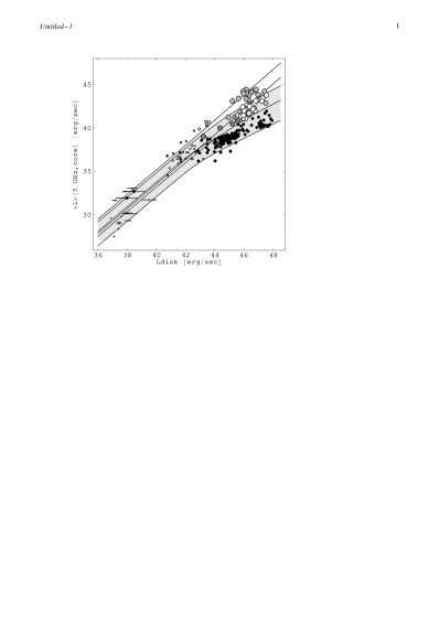
Figure 1: The correlation between thermal emission from the accretion disk (with the exception of X-rays this is basically normalized to their narrow H$\alpha$ emission) and the monochromatic luminosity of AGN radio cores, spanning the entire observed luminosity range. Open circles: Radio-loud quasars; small open circles: FR I radio galaxies; open gray circles: Blazars and radio-intermediate quasars (dark grey); black dots: radio-quiet quasars and Seyferts; small dots: X-ray binaries; small boxes: detected sources from the from the “48 LINERs” sample (Nagar et al. 2002). The shaded bands represent the radio-loud and radio-quiet jet models as discussed in Falcke & Biermann (1995)

Even though at these larger distances the jet pressure has decreased enough so that pressure balance between jet and external medium is reached, it is believed that the implied adiabatic losses are largely avoided by a constant re-collimation (Sanders 1983) of the jets: the side-ways lateral expansion leads to a re-collimation shock which in turn will focus the kinetic energy of the jet back into the forward direction. Otherwise one would have to account for expansion factors of $\mathrel{\hbox{\hbox to0.0pt{\hbox{\lower 4.0pt\hbox{$\sim$}}\hss}\hbox{$>$}}}10^{6}$ between launch and termination of powerful jets. For a relativistic plasma where adiabatic losses scale as $r^{-2/3}$ this would translate into an energy loss of four orders of magnitude and require the jets to start with enormous initial powers of $10^{49-51}$ erg/sec, corresponding to accretion rates of $10^{2-4}M_{\odot}$/yr and Eddington luminosities for black holes with a mass of $10^{10-12}M_{\odot}$. From all what we know today, this seems to be too high and one must conclude, that most of the way, the jet does not suffer adiabatic losses.

The argument based on hotspots still has the problem that it depends on parameters characterizing the external medium the jet is interacting with. If we go to low-power jets we will find that most of them (e.g., in FR I radio galaxies, Seyferts) do not even have hotspots that would provide one with a well-defined, isolated dissipation region to determine basic jet parameters easily. In the most extreme cases, however, even powerful jets are stopped inside a galaxy – either because they are young or because the ambient density is very high – and they appear as very compact radio galaxies of 0.1-10 kpc in size, named GHz-Peaked-Spectrum (GPS) sources or Compact-Steep-Spectrum (CSS) sources. The prospects for using such sources to discover the first black holes is discussed at the end of this paper.

Every jet, however, should also have an “inflationary phase” close to the nucleus, after leaving the nozzle where the energy density in powerful jets can be $1-100$ erg/cm³ and above, compared to $10^{-12}$ erg/cm³ in the local ISM. This is the region where flat spectrum radio cores are produced and which we will use in the following to make some quantitative statements. The advantage of radio cores is that they are largely independent of external conditions and therefore should be visible in basically all types of sources that produce relativistic jets. Their independence comes for a price, since less interaction often means less shocks, less energy dissipation, and less radio emission. Hence, compact radio cores are much more difficult to observe than extended lobes and jets, but modern radio astronomy is now sensitive enough to do just this.

2.1 Jet-Disk Coupling

In order to quantify the radio emission we expect from a radio jet close to the nucleus we will make a few assumptions and resort to the simple Ansatz made in Falcke & Biermann (1995), assuming that every jet is coupled to an accretion disk. A coupled jet-disk system has to obey the same conservation laws as all other physical systems, i.e. at least energy and mass conservation (other conservation laws we do not use yet). We can express those constraints by specifying that the total jet power $Q_{\rm jet}$ of the two oppositely directed beams is a fraction $2q_{\rm j}<1$ of the accretion power $Q_{\rm disk}=\dot{M}_{\rm disk}c^{2}$, the jet mass loss is a fraction $2q_{\rm m}<1$ of the disk accretion rate $\dot{M}_{\rm disk}$, and the disk luminosity is a fraction $q_{\rm l}<1$ of $Q_{\rm disk}$ ($q_{\rm l}=0.05-0.3$ depending on the spin of the black hole). The dimensionless jet power $q_{\rm j}$ and mass loss rate $q_{\rm m}$ are coupled by the relativistic Bernoulli equation (Falcke & Biermann 1995) for a jet/disk-system. For a large range in parameter space the total jet energy is dominated by the kinetic energy such that one has $\gamma_{\rm j}q_{\rm m}\simeq q_{\rm j}$, in case the jet reaches its maximum sound speed, $c/\sqrt{3}$, the internal energy becomes of equal importance and one has $2\gamma_{\rm j}q_{\rm m}\simeq q_{\rm j}$ (’maximal jet’). The internal energy is assumed to be dominated by the magnetic field, turbulence, and relativistic particles. We will constrain the discussion here to the most efficient type of jet where we have equipartition between the relativistic particles and the magnetic field and also have equipartition between the internal and kinetic energy (i.e. bulk motion) – one can show that other, less efficient models would fail to explain the highly efficient radio-loud quasars but also fail to explain radio cores in low-luminosity AGN.

Knowing the jet energetics, we can describe the longitudinal structure of the jet by assuming a constant jet velocity (beyond a certain point) and free expansion according to the maximal sound speed ($c_{\rm s}\mathrel{\hbox{\hbox to0.0pt{\hbox{\lower 4.0pt\hbox{$\sim$}}\hss}\hbox{$<$}}}c/\sqrt{3}$). For such a jet, the equations become very simple. The magnetic field is given by

$$B_{\rm j}=0.3\,G\;Z_{\rm pc}^{-1}\sqrt{q_{\rm j/l}L_{46}}$$ (1)

and the particle number density is

$$n=11\,{\rm cm}^{-3}L_{46}q_{\rm j/l}Z_{\rm pc}^{-2}$$ (2)

(in the jet rest frame). Here $Z_{\rm pc}$ is the distance from the origin in parsec (pc), $L_{\rm 46}$ is the disk luminosity in $10^{46}$ erg/sec, $2q_{\rm j/l}=2q_{\rm j}/q_{\rm l}=Q_{\rm jet}/L_{\rm disk}$ is the ratio between jet power (two cones) and disk luminosity which is of the order 0.1–1 (Falcke, Malkan, & Biermann 1995) and $\gamma_{\rm j,5}=\gamma_{\rm j}/5$ ($\beta_{\rm j}\simeq 1$). If one calculates the synchrotron spectrum of such a jet, one obtains locally a self-absorbed spectrum that peaks at

$$\nu_{\rm ssa}=20\,{\rm GHz}\;{\cal D}{\left(q_{\rm j/l}L_{46}\right)^{2/3}\over Z_{\rm pc}}\,\left({\gamma_{\rm e,100}\over\gamma_{\rm j,5}\sin i}\right)^{1/3}.$$ (3)

Integration over the whole jet yields a flat spectrum with a monochromatic luminosity of

$$L_{\nu} = {1.3\cdot 10^{33}}\,{{\rm erg}\over{\rm s\,Hz}}\;\left({q_{\rm j/l}L_{46}}\right)^{17/12}{\cal D}^{13/6}\sin i^{1/6}$$ (4)

$$\times\gamma_{\rm e,100}^{5/6}\gamma_{\rm j,5}^{11/6},$$

where $\gamma_{\rm e,100}$ is the minimum electron Lorentz factor divided by 100, and ${\cal D}$ is the bulk jet Doppler factor. At a redshift of 0.5 this luminosity corresponds to an un-boosted flux of $\sim 100$ mJy. The brightness temperature of the jet is

$${T}_{\rm b} = 1.2\cdot 10^{11}\,{\rm K}\;{\cal D}^{4/5}{\left({{\gamma_{\rm e,100}}^{2}q_{\rm j/l}L_{46}\over\gamma_{\rm j,5}^{2}\beta_{\rm j}}\right)^{1/12}}$$ (5)

$${\times\sin i^{5/6}}$$

which is almost independent of all parameters except the Doppler factor. A more detailed calculation of this can be found in Falcke & Biermann (1995).

A basic conclusion is that compact radio cores should exist essentially in all AGN, subject mainly to a range in accretion powers. Hence, we can expect many faint radio cores in nearby low-luminosity AGN (LLAGN) and a few bright radio cores in the most distant and brightest AGN that overall share almost the same properties: compact with a flat radio spectrum. This has been observationally verified by radio surveys of different types of black holes, starting at stellar masses and low powers (see Fender, this volume), via LLAGN (next section), all the way up to the brightest quasars. Figure 1 shows radio core fluxes as a function of optical/X-ray luminosity, illustrating the enormous range compact radio cores occupy.

2.2 Power Unification

Figure 1 seems to indicate that the radio luminosity of black holes simply scales with the thermal component, i.e. the accretion disk luminosity. However, the actual picture is more complicated as accretion flows and their related emission may not show a simple linear scaling. Recent results suggest that accreting black holes can exist in mainly two distinct states. Which state it is in depends mainly on the accretion rate. In the low-power state the standard optically thick disk is probably truncated and a radiatively inefficient optically-thin accretion flow exists in the inner regions of the flow (see e.g., Esin et al. 1997, Poutanen 1998). In the high state the optically-thick geometrically thin accretion flow seems to continue to the innermost stable orbit. For XRBs the transition appears to happen at an accretion rate of roughly 10% Eddington (see e.g., Narayan & Yi 1995). Recent work suggests that this transition can already happen at 2% of the Eddington rate (Maccarone 2004), and that there is a hysteresis in the critical accretion rate depending on which direction the transition is going along (Maccarone & Coppi 2003, Fender & Belloni 2004). For AGN the position of the transition is also compatible with a few percent Eddington (Ghisellini & Celotti 2001).

At least the low power state is normally connected with relativistic outflows. As mentioned above the jet will contribute significantly to the SED for XRBs and AGN (Falcke & Markoff 2000, Markoff et al. 2001, Fender 2001, Yuan, Markoff, Falcke 2002). As the accretion flow is radiatively inefficient in the innermost regions the jet can even dominate the overall emission (see e.g., Fender, Gallo, Jonker 2003, Falcke et al. 2004). This concept of jet-domination can be used to unify stellar and super-massive black holes.

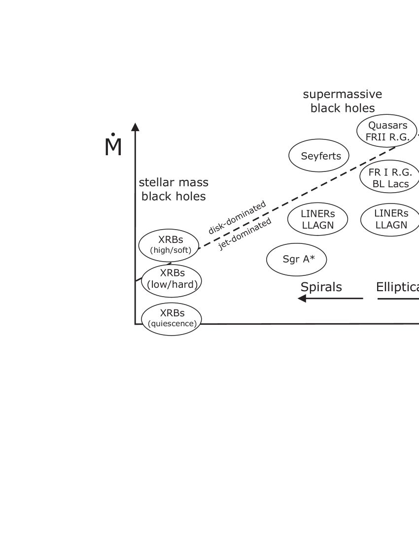
Figure 2: A proposed unification scheme for accreting black holes in the mass and accretion rate plane. Above a few percent of the Eddington accretion rate, the systems are proposed to be dominated by disk emission, while below they are inherently dominated by jet emission (RG=radio galaxy). This unification scheme extends the standard inclination-based unified schemes (Antonucci 1993, Urry Padovani 1995).

The main assumptions used for the unification scheme are:

1. The jet and the accretion flow is a coupled symbiotic system. If one of them exists the other will also be present (e.g., Falcke & Biermann 1995).

2. Below a critical accretion rate $\dot{M}_{\mathrm{crit}}$ which is a small fraction of the Eddington accretion rate, the innermost parts of the accretion flow become radiatively inefficient.

3. For $\dot{M}\leq\dot{M}_{\mathrm{crit}}$ the overall emission will be dominated by the jet.

This requires a better classification of AGN into disk or jet dominated classes and a single basic SED cannot be assumed. As mentioned above black hole XRBs appear mainly in two distinct states: the low/hard state characterized by a hard power-law (e.g., Nowak 1995) and the high state where the SED is dominated by a thermal component. The hard power-law of the low-hard state is often explained by Comptonization in a hot corona or the optically thin accretion flow (see, e.g. Shapiro, Lightman, & Eardley 1976, Sunyaev & Trümper 1979) but can also be explained as synchrotron emission from a relativistic jet (Markoff et al. 2001). The latter interpretation is further supported by the finding of a fairly universal radio/X-ray correlation in the low/hard state (Gallo, Fender, & Pooley 2003) which can be well explained with a jet model (e.g., Markoff et al. 2003, Falcke et al. 2004). Thus, we identify the low/hard state as jet-dominated while the soft state is assumed to be disk-dominated. As there are many different classes of AGN the classification in disk/jet dominated sources is more complicated than for the stellar counterparts. The current classification is summarized in Fig. 2. For a more detailed analysis see Falcke et al. (2004).

2.3 The Radio/X-ray correlation

Clearly, if the SED is dominated by one component – suggested for the jet-dominated low-power system, different wavelengths should be related in a defined manner, subject to scaling with mass and accretion rate. This can be used to predict which wavelength range is best for detecting certain types of AGN; vice versa one could also say that every wavelength range somehow pre-selects certain ranges in mass and accretion rate.

For example, it has been found recently that radio and X-rays from black holes are correlated in a very specific, mass-dependent manner (Falcke et al. 2004; see also Merloni, Heinz, & di Matteo 2003). This can be easily understood using the jet domination idea, where the radio is from the optically thick part of the spectrum, while X-rays come from the optically thin part (other explanations have also been put forward, however). Using scaling laws for the jet SED it can then be shown that the X-ray luminosity is expected to depend on the radio luminosity and the black hole mass, $M_{\bullet}$, as:

$$L_{\rm X}\propto L_{\rm R}^{1.38}M_{\bullet}^{0.81}.$$ (6)

Of course, for many AGN the X-ray emission probably does not originate from synchrotron processes, still the correlation seems to be applicable for a large range of sources. If one corrects for the mass dependence of the X-ray/radio correlation according to Eq. 6 one finds a universal radio/X-ray correlation for all jet dominated sources from XRBs up to AGN as shown in Fig. 3. Put differently: optically thick (radio) emission, optically thin (X-rays or optical) emission, and black hole mass form a fundamental plane for low-power black holes.

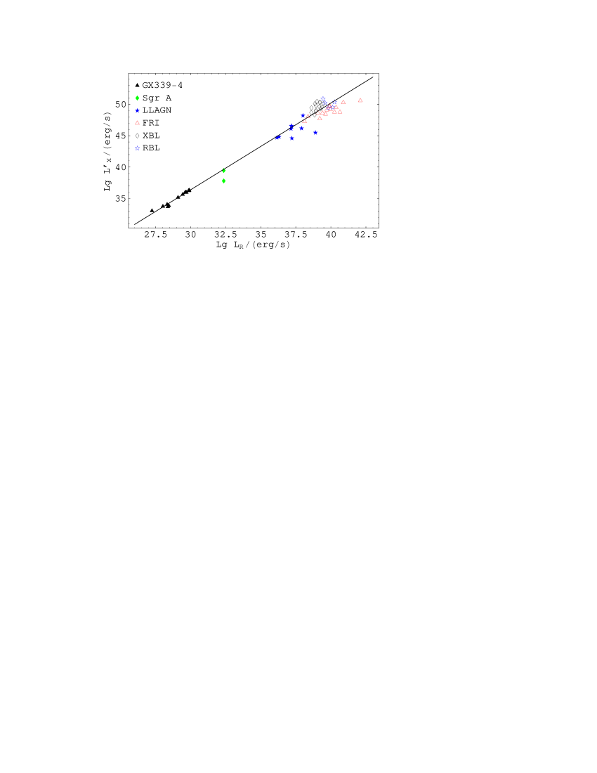
Figure 3: Radio/equivalent X-ray correlation for a sample of jet dominated AGN and XRBs. The X-ray flux has been adjusted to correspond to a black hole mass of 6$M_{\odot}$.

2.4 Observational Consequences

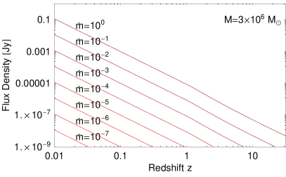
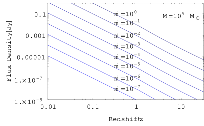
Figure 4: Predicted fluxes of radio cores in AGN observed at 5 GHz as a function of redshift for a range of Eddington accretion rates (solid lines from top to bottom) and two black hole masses: $3\times 10^{6}M_{\odot}$ (left) and $10^{9}M_{\odot}$ (right). An inclination angle of $50^{\circ}$ is assumed, i.e. negligible beaming.

From the radio/X-ray correlation we can already deduce which compact sources we can expect to observe with the SKA at radio frequencies.

• XRBs: Compared with AGN all XRB are X-ray loud (up to a factor $10^{8}$ more X-ray flux for a given jet power), but relatively weak in the radio regime hence X-ray telescopes are better suited for low-mass black holes. However, as the radio flux can be relativistically beamed in some sources the SKA will allow us to observe these sources not only in our Galaxy, but also in nearby galaxies.

• AGN: With their large total jet power and high black hole masses these sources can be radio-loud. Additional relativistic beaming allows the detection of AGN up to very high redshifts. The SKA will boost AGN research, as it will allow to observe AGN of lower luminosities and at larger distances.

• Intermediate mass black holes (IMBHs): If this intriguing class of objects should exist it would lie in between AGN and XRBs on the radio/X-ray correlation. With new generation radio telescopes these objects should be visible in nearby galaxies. As Maccarone (2004) points out, IMBHs in the center of globular clusters are easier detected in the radio regime. Their X-ray luminosity would be further reduced as low accretion rate systems might not start accelerating relativistic particles (e.g. Sgr A^∗ in its quiescent state).

In Fig. 4 we show predicted radio core fluxes as a function of redshift for a range of radio core models at 5 GHz and for different masses and accretion rates relative to the Eddington rate. The fluxes are predicted on the basis of Eq. 4 for an inclination angle of $i=50^{\circ}$ and taking the mass scaling into account as discussed in Falcke et al. (2004). The left figure corresponds to a black hole similar to Sgr A* in the Milky Way (see, e.g., Melia & Falcke 2001) and the right one to a black hole in a massive elliptical galaxy. The bottom line on the left corresponds to the activity level in Sgr A*, while the top one on the right corresponds to a bright radio-loud quasar. Assuming that the SKA, after long integration, can reach levels as low as 10 nJy, we see that Sgr A*-like objects, i.e., essentially every supermassive black hole in the local universe, can be detected out to 40 Mpc.

Quasar radio cores, on the other hand, can essentially be seen all the way out to redshifts of $z>30$. For a survey with detection limits around 0.1 $\mu$Jy we can even see black holes in normal galaxies shining at the Eddington rate out to $z\simeq 8$. Assuming that the formation of galaxies proceeds rapidly in the early phases of the universe at $z>10$ and black holes accrete at the Eddington limit, we could in principle see the associated radio cores as soon as a mass of $10^{7}M_{\odot}$ is reached. In section 4 we will, however, discuss another possibility to detect black holes in the making. Note that the predictions made here only assumed an average inclination angle. Obviously, some of these sources will be beamed and hence a few lower mass black holes could be seen as well as flat-spectrum sources. A crucial prerequisite is, of course, the presence of sensitive long baselines in the SKA, to isolate the high-brightness temperature cores from diffuse star formation.

3 SKA and the Weak AGN Tail

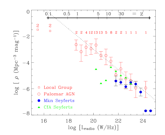
Figure 5: The 15 GHz nuclear radio luminosity function (RLF) of the 150 mas-scale radio nuclei in the Palomar sample (red open circles, with the number of galaxies in each bin listed above the symbol) as compared to the RLFs for Markarian Seyferts (RLF from Meurs & Wilson 1984) and CfA Seyferts (RLF calculated by Ulvestad & Ho (2001) using data from Kukula et al. 1995). The dashed line is a power-law ($-0.78$) fit to the Palomar RLF (excluding the two lowest radio luminosity points). Also shown is the estimated nuclear RLF of galaxies in the local group (red squares, with 2 galaxies in each of the two bins; see text). The upperscale illustrates the detection limits of the SKA (using an r.m.s noise of 0.3$\mu$Jy in 1 hr of imaging, and a 3$\sigma$ detection threshold) of similar AGNs at redshifts of 0.1 to 30.

Some idea of the high-z AGN population accessable to SKA can be obtained from extrapolating deep radio surveys of local AGNs. Currently the deepest radio search for AGNs in a large well-defined sample of nearby galaxies is a VLA and VLBA survey of the Palomar sample of all $\sim$480 nearby bright (B${}_{\rm T}\,<$12.5 mag) northern galaxies. Optical spectroscopy of the sample (Ho, Filippenko, & Sargent 2003) shows that it is made up of roughly 197 AGNs (almost all with L${}_{\rm H\alpha}~{}\leq$ 10⁴⁰ erg s^-1, i.e. low-luminosity AGNs or LLAGNs) 206 nuclei with H II type nuclear spectra, and 53 absorption line nuclei. Effectively all galaxies have been surveyed to detection limits of 1 mJy with the VLA (15 GHz; 0$.\!\!^{\prime\prime}$15 resolution), with follow-up VLBA observations (5 GHz, 2 mas resolution) confirming the AGN nature of all VLA detections with flux $>$2.7 mJy (Falcke et al. 2000, Nagar et al. 2004).

Most of the $\sim$70 VLA-detected radio nuclei are compact or at least the AGN-related radio emission is primarily from within the central arcsec. The radio detected nuclei have been used to derive a nuclear, i.e. AGN core 15 GHz radio luminosity function (RLF) which is plotted in Fig. 5 as open red circles; see also Ulvestad & Ho (2001, RLF for Palomar Seyferts), and Filho (2003, $PhD$ thesis; RLF for Palomar sample using diverse radio surveys). At the highest luminosities the RLF is in good agreement with that of ‘classical’ Seyferts (Fig. 5). We use the other RLFs without correction for frequency or nuclear vs. total AGN emission since our RLF is derived from nuclei which show relatively flat radio spectra from 1.4–15 GHz and which are relatively compact (i.e. sub-arcsec). At lower luminosities, the sample extends the RLF of AGNs by more than three orders of magnitude. A fit to the Palomar RLF (excluding the two lowest luminosity bins; see below) yields:

$${\log}\rho = \left(12.5-0.78\times\,{\rm log}\,\left({\rm L}_{\rm radio}\,[{\rm W\,Hz}^{-1}]\right)\right)$$ (7)

$$[{\rm Mpc}^{-3}\,{\rm mag}^{-1}]$$

An approximate RLF for the nuclei of the local group of galaxies is also plotted in Fig. 5. At $\sim 10^{15}$ W Hz^-1 one has two galaxies: the Milky Way and M 31. At $\sim 10^{16}$ W Hz^-1, NGC 205 and NGC 598 (see Nagar et al, 2004). These lowest points, and our extrapolations of the radio non-detections, support a lower power turnover for the RLF, though the apparent turnover could also be due to the incompleteness of the radio survey.

The upper bar in Fig 5 illustrates the detection limits of the SKA (using an r.m.s noise of 0.3$\mu$Jy in 1 hr of imaging, and a 3$\sigma$ detection threshold) of a similar sample of AGNs at redshifts of 0.1 to 30. The most luminous sources here would be detectable out to $z\,=\,30$, while at $z\,=\,0.1$ radio nuclei in AGNs can be detected down to levels of 10 times Sgr A^∗. We have used these SKA detection limits, in combination with our RLF and the SDSS galaxy luminosity function (determined for z$\,=\,0-3.5$) to estimate the number of AGNs identified by the SKA (assuming a VLBI SKA, so as to easily distinguish AGN from starbursts) and compared these with several large optical and hard X-ray surveys (Fig. 6). The AGN counts for these other surveys were estimated from their total galaxy counts in conjunction with intial results on the incidence of AGN in those surveys. Clearly, an SKA survey will find an unprecedented number of AGNs over all redshift ranges.

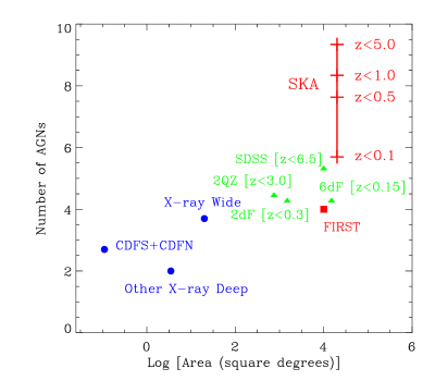
Figure 6: A comparison of the number of AGNs expected to be identified by several current large area or deep surveys as a function of their sky coverage. The typical redshift limit probed by the survey is also marked in some cases. X-ray surveys in blue: CDFS and CDFN are the Chandra Deep Field North and South. “X-ray wide” indiactes a shallow X-rays survey with a much wider field of view. Optical surveys in green: these consist of the Two-degree-field galaxy redshift survey (2dF), the Two-degree-field QSO survey (2QZ), the Six-degree-field survey (6dF) and the Sloan Digital Sky Survey (SDSS). Radio surveys in red; the predicted number counts for a VLBI-SKA ‘one-hemisphere’ survey (1 hr per pointing) out to different redshifts are indicated.

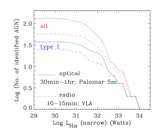
Figure 7: The cumulative number of ‘definite’ (i.e. those detected in the hard X-ray) AGNs identified by optical spectroscopy (solid lines; $\sim$4 hr on the Palomar 5 meter) and radio imaging (dashed lines; $\sim$20 min at the VLA), as a function of the luminosity of the narrow H$\alpha$ line. The blue lines are for only type 1 nuclei (i.e. nuclei with broad H$\alpha$ emission) and the red lines for both type 1 and type 2 nuclei.

The effectiveness of the SKA in detecting AGN is illustrated above and in the previous section. However, it is also valid to ask how complete such an AGN sample would be, both intrinsically, and as compared to X-ray or optically identified AGN. To illustrate the effectiveness of radio surveys for AGNs at the lowest luminosities, we plot (Fig. 7) the cumulative number of definite AGNs (here we take the presence of a hard X-ray source as a definite sign of AGN activity) identified by optical spectroscopy (typically 4 hr on a 5 meter telescope) versus radio imaging (typically 20 min at the VLA). Clearly, the radio survey picks up a highly significant fraction of definite AGNs, and in fact, in the absence of hard X-ray data is a more reliable indicator of true AGN activity than optical spectroscopy, especially at these low luminosities.

4 The First Black Holes

4.1 HI spectroscopy

One of the big goals of the SKA, however, is the identification of the very first and hence youngest black holes in the universe. This requires detecting them in the redshift range 7–20. Conventional optical spectroscopy becomes difficult in this regime due to the pronounced Ly$\alpha$ troughs (e.g., Becker et al. 2001). Therefore, the prospects of radio spectroscopy, using the 21 cm hydrogen line, at very high-redshifts has become an important topic for the next generation of radio telescopes. Carilli, Gnedin, & Owen (2002) discuss the detectability of HI absorption towards radio galaxies at redshifts $z=8-10$. The conclusion is that depending on the quasar evolution model hundreds to thousands of bright QSOs should be detectable at these redshifts in the radio, assuming radio powers comparable to Cygnus A and black hole masses as high as several $10^{9}M_{\odot}$.

Of course, even with the SKA detecting these early black holes is not an easy task, requiring a lot of integration time. Given that the SKA will be able to see essentially every radio galaxy that has existed within the accessible universe, the number of candidate sources is enormous and effective survey and selection criteria have to be developed. After all, one of the big advantages (and curses) of SKA will be its powerful surveying capability due to its large field of view.

Consequently, we have to discuss how the first black holes will look like and what would distinguish them from other radio sources. While such an attempt will always be speculative it is not futile. In contrast to the formation of the first stars, the energy release from black holes is primarily release of gravitational energy and not due to nuclear synthesis. Unknown metallicity effects should not play as much a role as it will for the first stars. This is even more true for the radio emission which comes from a hot, fully ionized, and relativistic plasma. We can thus expect that the appearance of the first black holes themselves will not be very much different from what we see today. Modifications in the appearance are mainly expected from cosmological effects (extreme redshift), a denser ambient photon field (inverse Compton cooling), and a different – presumably much denser – environment in the emerging nuclei of forming galaxies.

In section 2.4 we discussed how the inner parts of the jet, the radio core, can be detected. In the following we will concentrate more on the extended emission, even though this could be confined to compact scales as well, as we argue below.

4.2 High-redshift radio galaxies

Figure 8: Radio spectral index plotted against redshift for 108 radio galaxies. Filled dots are from the ultra-steep spectrum (USS) sample of Röttgering et al. (1997). The spectral indices are determined between the lowest available frequency above 150 MHz and 5 GHz. The open circles are also from the Röttgering et al. (1997) USS sample with redshifts obtained at Lick Observatory by McCarthy & van Breugel (1994, private communication). The crosses ($\times$) are from the Molonglo sample of McCarthy (1990a,1990b), the pluses ($+$) are Bologna sources (McCarthy 1991, Lilly 1988), the triangles are from the 8C survey (Lacy et al. 1994, Lacy 1992) and the diamond is 6C 1232+39 (Eales & Rawlings 1993). Figure reproduced from Röttgering et al. (1997) – Astronomy & Astrophysics

One fairly successful technique to find high redshift radio galaxies has been to select on steep spectral indices. The radio emission from typical radio galaxies is normally dominated by optically thin synchrotron emission from their lobes. The spectral index in the radio then reflects the particle energy distribution; both are a power law over a wide range of energies, respectively frequencies. Beyond a certain break energy and frequency the power law steepens due to cooling losses. Clearly, with higher redshifts this steepening will occur at lower and lower observing frequencies. In addition the higher photon density in earlier epochs may lead to enhanced cooling and lower break frequencies such that high-z radio galaxies appear to have steeper spectra. A similar effect is expected if the radio source spectra have a curved intrinsic shape as discussed, for example, by Blundell, Rawlings, & Willott (1999).

Various surveys (see, e.g., Röttgering 1997) indicate that indeed spectral index and redshift are correlated (Fig. 8). Standard selection procedures are to compare radio surveys at two or more frequencies, select the ones with steeper spectral index ($\alpha<-1$, where the flux density as a function of frequency is $S_{\nu}\propto\nu^{\alpha}$), determine their structure and position with arcsecond-resolution radio observations, and obtain their spectral index with optical spectroscopy. The latter part is a tedious process and may become prohibitive for the large number of sources the SKA is going to provide. Moreover, it is not clear whether the trend of steeper spectral index with higher redshift continues, especially as the spectral index also depends on size and power of a radio galaxy (e.g., Dennett-Thorpe et al. 1999). Still, with its large spectral and instantaneous bandwidth coverage the SKA will deliver a huge number of ultra-steep spectrum sources and very interesting high-z candidates (see chapter by Jarvis & Rawlings, this volume).

4.3 The Very First Black Holes

However, one can ask whether indeed all these arguments apply to the very first generation of black holes – those where galaxy and central black hole are in the process of being formed. The growth process of black holes can be rather rapid – within 300-600 Million years a black hole can grow to more than $10^{9}M_{\odot}$ if it accretes at the Eddington rate. As argued in section 2.4 this means even at $z>10$ the compact radio emission from inner jets can be seen; however, what happens to the extended emission?

Given that the densities of the ISM in the host galaxy must be extremely high, it is not clear that the jets will be able to even penetrate into the – also very dense – intergalactic medium. If so, the jet will develop very strong and very bright hot spots inside the forming galaxy similar to what we see in GPS sources.

GPS sources show a highly peaked spectrum in the GHz regime, where the deficiency at low frequencies is most likely due to synchrotron self-absorption, only in a few cases free-free absorption also contributes. Hotspots, if understood as homogenous synchrotron sources, should follow some simple relations. Especially, one expects that the turn-over (or the self-absorption) frequency decreases with increasing size. This can be seen in studies of samples and even in individual sources – very impressively for example in the evolution of the radio hotspots of III Zw 2, peaking at 43 GHz (Brunthaler et al. 2003).

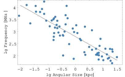
Figure 9: The intrinsic turnover frequency vs. linear size of radio sources in the Fanti et al. (1990) CSS sample and the Stanghellini et al. (1996) GPS sample. Adapted from O’Dea & Baum (1997) and O’Dea (1998).

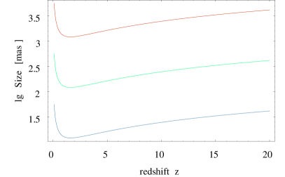
Figure 10: Within a standard cosmology ($\Omega_{\rm m}=0.3$, $\Omega_{\lambda}=0.7$, $H_{0}=72$ km/sec/Mpc) a fixed angular size (left) and peak frequency (right) of a source scale differently as a function of redshift. The figure shows three examples for sources with 0.1 (blue), 1 (green), and 10 kpc (red) size, and their respective peak frequencies according to Eq. 8. This exemplifies the typical range of GPS and CSS sources.

For GPS sources at lower redshifts (i.e. around unity), O’Dea (1998) and Snellen et al. (2000) found a number of relations that relate power, size $l$, and turn-over frequency $\nu_{\rm peak}$ of GPS sources. The best relation exists between size and turn-over frequency as shown in Figure 9. Converted to parameters intrinsic to the source this can be fitted by an expression of the form

$$\nu_{\rm peak}=10^{(-0.21-0.65\times\lg{({l/{\rm kpc}})})}\;{\rm GHz},$$ (8)

which essentially reflects some basic properties of synchrotron theory.

Similarly, one could expect that the synchrotron power is related to the turnover frequency or the size. However, O’Dea (1998) could not identify a clear trend. The monochromatic power at 5 GHz for currently known GPS and CSS sources is rather constant with a large scatter. On the other hand, Snellen et al. (2000) see a trend of decreasing flux density with increasing size. For simplicity we here consider a constant power at 5 GHz of $L_{\rm 5GHz}=10^{27.25}$ W/Hz in the restframe frequency and only take redshift into account assuming a spectrum with $\alpha=-0.6$.

It is now interesting to see how GPS sources would look like as a function of redshift. In this respect it is important to note that angular sizes transform differently than frequencies. Obviously, for a fixed GPS source the turn-over frequency will monotonically decrease with increasing redshift. On the other hand, for a modern cosmology the angular size will decrease and later increase again at very high $z$. This markedly different behavior is illustrated in Fig. 10 where we place three example GPS and CSS sources at different redshifts obeying relation 8. If we take a standard GPS source peaking at 2.7 GHz and 100 pc size, it would appear as a compact source of 40 mas at $z\,=$ 20 – quite common for GPS sources – but unusually low turn-over frequency of 125 MHz, something that is more expected for much larger CSS sources. Of course, a source at that redshift would also be much fainter than “local” GPS/CSS sources.

We can combine the three measurables: angular size $\theta$, observed frequency $\nu_{\rm peak,obs}$, and flux density in one diagram. One can easily see from Eq. 8 that the product of $\nu_{\rm peak,obs}^{\beta}\times\theta$ should be constant for $\beta=1/0.65=1.54$. Obviously, that parameter may have to be changed once a better relation has been established. Using the Fanti et al. (1990) CSS sample and the Stanghellini et al. (1996) GPS samples with $\nu_{\rm peak}>100$ MHz we find that indeed all sources cluster around $\left<\nu_{\rm peak,obs}^{1.54}\times\theta\right>=10^{6.2\pm 0.4}\;{\rm mas}\times{\rm MHz}^{1.54}$, i.e. despite their wide range in sizes and peak frequencies the sample collapses to a cloud of sources within one order of magnitude (Fig. 11).

We can then combine the predicted sizes and peak frequencies as a function of redshift from Fig. 10, combine them in the same manner and overplot them on the data, extending all the way out to high redshifts. While the current GPS/CSS sources cluster in the top right corner, extremely high-redshift GPS/CSS are expected to cluster in the bottom left corner – the discovery space for the SKA.

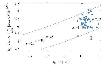
Figure 11: Size, frequency, and flux density roughly form a fundamental plane for GPS radio galaxies. Here we plot a combination of frequency and size ($\nu_{\rm peak}^{1.54}\times r$) vs. the flux density for a range of empirical GPS models and actual GPS sources from O’dea (1998). Size and frequency for the model are coupled according to Eq. 8 for sources with different sizes of 0.1 (blue), 1 (green), and 10 kpc (red) and fall on top of each other. The two lines delimit the scatter in the empirical relation. The labels indicate the typical redshift of sources in that regime. Standard GPS sources are found in the redshift range around z=1. The bottom left corner is not occupied and is the discovery space for young high-redshift black holes with the SKA.

What are the pitfalls of such a scenario? It could be that the basic relation between size and frequency changes. This is not really expected if the turn-over is caused by synchrotron-self absorption, as the same physics should also apply at z=20. Modifications, however, would be required if free-free absorption becomes important – something that cannot be excluded in the violent early phase of galaxy formation. On the other hand, free-free absorption in a stratified atmosphere should lead to a qualitatively and perhaps even quantitatively similar behavior. Inverse Compton cooling from ambient photons might also change the state of synchrotron sources. However, many GPS sources are found in very luminous quasars and hence are generally already exposed to a bright photon field. Finally, there could be confusing sources. We know very little about the GPS/CSS population at lower luminosities and the faint part could be heavily confused by local low-luminosity AGN. Still, even in this case we expect a markedly different size/frequency ratio than for sources at very high redshifts as the size-frequency relation does not depend strongly on power. Also, nearby galaxies could be easily excluded through cross-correlation with existing optical catalogs.

A survey strategy for finding the first black holes would then be:

• a shallow all-sky multi-frequency survey in the range 100-600 MHz down to 0.1 mJy at arcsecond resolution,

• identification of compact, highly peaked spectrum sources in that frequency range,

• identification of empty fields in the optical,

• re-observation to exclude variable sources,

• observation with long baselines and resolutions of $\sim$ 10 mas to determine sizes and to pick out the ultra-compact low-frequency peaked (ULP) sources,

• spectroscopic confirmation of remaining candidates with HI observations or by other means.

The SKA would be ideally suited for all these tasks. With a large field of view, a broad instantaneous frequency coverage, and multibeaming it would be very efficient in making the first surveys and generating a candidate source list of faint, low-peaked sources. Long baselines are then essential to confirm the AGN nature and the unusual angular sizes expected.

5 Summary

In this paper we have discussed the prospects to detect and discover black holes throughout the universe with the SKA. We have concentrated on the compact, high-brightness temperature emission as this most easily distinguishes black hole activity from other processes. This radio emission is typically produced by relativistic radio jets and is present in essentially all AGN at some level. The radio emission is correlated with the X-ray emission, the accretion rate, and the mass of the black hole. Supermassive black holes are best found in the radio while stellar mass black holes are better picked up in the X-rays. Compact jet emission seems to be more “faithful” for sub-Eddington black holes and is a good tracer for faint black hole activity in the local universe. With the SKA we can thus detect essentially all black holes, even those as dormant as our Galactic Center, out to 40 Mpc. Moderate low-luminosity AGN can be seen out to $z=1$ and quasars near the Eddington limit can be seen well through the Epoch of Reionization. If black holes in the range $10^{7-9}M_{\odot}$ form through accretion near the Eddington limit at redshifts $z>10$, their cores can be picked up when they have reached a mass of $10^{7}M_{\odot}$. This only considers the high-brightness temperature radio cores without the extended emission and does not require beaming which would make even fainter black holes visible.

An interesting question is whether and how the SKA can actually identify the very first generation of black holes. Bright radio galaxies could be used as tracers and one could search for extremely steep spectra and/or HI absorption in the Epoch of Reionization. However, we suggest that the first radio jets might rather look like GPS/CSS sources with compact hot-spots as they are stopped in the presumably dense interstellar medium of early galaxy formation. They would reveal themselves through a low-frequency turn-over in the spectrum due to synchrotron self-absorption and a very compact (some ten mas) size. Since size and frequency of GPS sources are correlated but angular size and frequency scale markedly differently at high redshifts, the very first black holes should occupy a rather unique place in a parameter space spanned by size, turn-over frequency, and flux density. Discovering such sources requires a broad bandwidth, good surveying capabilities (large field-of-view and multi-beaming), and long baselines to measure sizes in follow-up observations on a scale of tens of milliarcseconds. There is, in fact, a significant chance that, due to the absorption in the IGM in the epoch of reionization and within the assembling host galaxy, such radio surveys with the SKA are actually the only way to find the very first supermassive black holes in the universe.

References

- Antonucci (1993) Antonucci R., 1993, ARA&A, 31, 473
- Becker et al. (2001) Becker, R. H., et al. 2001, AJ, 122, 2850
- Blundell, Rawlings, & Willott (1999) Blundell, K. M., Rawlings, S., & Willott, C. J. 1999, AJ, 117, 677
- Brunthaler et al. (2003) Brunthaler, A., Falcke, H., Bower, G. C., Aller, M. F., Aller, H. D., Teräsranta, H., & Krichbaum, T. P. 2003, Publications of the Astronomical Society of Australia, 20, 126
- Buras, Rampp, Janka, & Kifonidis (2003) Buras, R., Rampp, M., Janka, H.-T., & Kifonidis, K. 2003, Physical Review Letters, 90, 241101
- Blundell, Rawlings, & Willott (1999) Blundell, K. M., Rawlings, S., & Willott, C. J. 1999, AJ, 117, 677
- Carilli, Gnedin, & Owen (2002) Carilli, C. L., Gnedin, N. Y., & Owen, F. 2002, ApJ, 577, 22
- Condon (1989) Condon, J. J. 1989, ApJ, 338, 13
- Dennett-Thorpe, Bridle, Laing, & Scheuer (1999) Dennett-Thorpe, J., Bridle, A. H., Laing, R. A., & Scheuer, P. A. G. 1999, MNRAS, 304, 271
- Esin et al. (1997) Esin A. A., McClintock J. E., Narayan R., 1997, ApJ, 489, 865
- Falcke & Biermann (1995) Falcke H., Biermann P. L., 1995, A&A, 293, 665
- Falcke, Körding, & Markoff (2004) Falcke, H., Körding, E., & Markoff, S. 2004, A&A, 414, 895
- Falcke, Malkan, & Biermann (1995) Falcke, H., Malkan, M. A., & Biermann, P. L. 1995, A&A, 298, 375
- Falcke & Markoff (2000) Falcke, H. & Markoff, S. 2000, A&A, 362, 113
- Falcke et al. (2000) Falcke, H., Nagar, N. M., Wilson, A. S., & Ulvestad, J. S. 2000, ApJ, 542, 197
- Fan et al. (2003) Fan, X., et al. 2003, AJ, 125, 1649
- (17) Fanti, R., Fanti, C., Schilizzi, R. T., Spencer, R. E., Rendong, N., Parma, P., van Breugel, W. J. M., & Venturi, T. 1990b, A&A, 231, 333
- Fender (2001) Fender R. P., 2001, MNRAS, 322, 31
- (19) Fender R. P., & Belloni, T., 2004, ARA&A, 42, 317-364
- Fender et al. (2003) Fender R. P., Gallo E., Jonker P. G., 2003, MNRAS, 343, L99
- Ferrarese & Merritt (2000) Ferrarese, L. & Merritt, D. 2000, ApJ, 539, L9
- Fossati et al. (1998) Fossati G., Maraschi L., Celotti A., Comastri A., Ghisellini G., 1998, MNRAS, 299, 433
- Gallo et al. (2003) Gallo E., Fender R. P., Pooley G. G., 2003, MNRAS, 344, 60
- Gebhardt et al. (2000) Gebhardt, K., et al. 2000, ApJ, 539, L13
- Ghisellini & Celotti (2001) Ghisellini G., Celotti A., 2001, A&A, 379, L1
- Gursky & Schwartz (1977) Gursky H., Schwartz D. A., 1977, ARA&A, 15, 541
- Ho et al. (1997) Ho, L. C., Filippenko, A. V., & Sargent, W. L. W. 1997a, ApJS, 112, 315
- Ho, Filippenko, & Sargent (2003) Ho, L. C., Filippenko, A. V., & Sargent, W. L. W. 2003, ApJ, 583, 159
- Kogut et al. (2003) Kogut, A., et al. 2003, ApJS, 148, 161
- Kukula et al. (1995) Kukula, M. J., Pedlar, A., Baum, S. A., & O’Dea, C. P. 1995, MNRAS, 276, 1262
- Maccarone (2004) Maccarone, T. J. 2004, MNRAS, 351, 1049
- Maccarone (2003) Maccarone T. J., 2003, A&A, 409, 697
- Maccarone & Coppi (2003) Maccarone T. J., Coppi P. S., 2003, MNRAS, 338, 189
- Markoff et al. (2001) Markoff S., Falcke H., Fender R., 2001, A&A, 372, L25
- Markoff et al. (2003) Markoff S., Nowak M., Corbel S., Fender R., Falcke H., 2003, A&A, 397, 645
- Melia & Falcke (2001) Melia F., Falcke H., 2001, ARA&A, 39, 309
- Merloni et al. (2003) Merloni A., Heinz S., di Matteo T., 2003, MNRAS, 345, 1057
- Meurs & Wilson (1984) Meurs, E. J. A. & Wilson, A. S. 1984, A&A, 136, 206
- Mirabel & Rodríguez (1999) Mirabel I. F., Rodríguez L. F., 1999, ARA&A, 37, 409
- Nagar et al. (2000) Nagar, N. M., Falcke, H., Wilson, A. S., & Ho, L. C. 2000, ApJ, 542, 186
- Nagar et al. (2002) Nagar, N. M., Falcke, H., Wilson, A. S., & Ulvestad, J. S. 2002, A&A, 392, 53
- Nagar et al. (2004) Nagar, N. M., et al, 2004, A&A, submitted
- Narayan & Yi (1995) Narayan R., Yi I., 1995, ApJ, 452, 710
- Nowak (1995) Nowak M. A., 1995, PASP, 107, 1207
- O’Dea (1998) O’Dea C. P., 1998, PASP, 110, 493
- (46) O’Dea, C. P., & Baum, S. A. 1997, AJ, 113, 148
- Portegies Zwart et al. (2004) Portegies Zwart, S. F., Baumgardt, H., Hut, P., Makino, J., & McMillan, S. L. W. 2004, Nat., 428, 724
- Poutanen (1998) Poutanen J., 1998, in Theory of Black Hole Accretion Disks, Cambridge University Press, p. 100
- Rawlings & Saunders (1991) Rawlings S., Saunders R., 1991, Nat., 349, 138
- Sandage, Tammann, & Yahil (1979) Sandage, A., Tammann, G. A., & Yahil, A. 1979, ApJ, 232, 352
- Sanders (1983) Sanders R. H., 1983, ApJ, 266, 73
- Shakura & Sunyaev (1973) Shakura N. I., Sunyaev R. A., 1973, A&A, 24, 337
- Shapiro et al. (1976) Shapiro S. L., Lightman A. P., Eardley D. M., 1976, ApJ, 204, 187
- Silk & Rees (1998) Silk, J. & Rees, M. J. 1998, A&A, 331, L1
- Snellen et al. (2000) Snellen, I. A. G., Schilizzi, R. T., Miley, G. K., de Bruyn, A. G., Bremer, M. N., & Röttgering, H. J. A. 2000, MNRAS, 319, 445
- (56) Stanghellini, C., Dallacasa, D., O’Dea, C. P., Baum, S. A., Fanti, R., & Fanti, C. 1996, in: Proc. Second Workshop on Gigahertz Peaked-Spectrum and Compact Steep-Spectrum Radio Sources, ed. I. A. G. Snellen, R. T. Schilizzi, H. J. A. R ttgering, & M. N. Bremer (Leiden: Leiden Obs.), 4
- Sunyaev & Trümper (1979) Sunyaev R. A., Trümper J., 1979, Nat., 279, 506
- Ulvestad & Ho (2001) Ulvestad, J. S. & Ho, L. C. 2001, ApJ, 558, 561
- Urry & Padovani (1995) Urry C. M., Padovani P., 1995, PASP, 107, 803
- von Montigny et al. (1995) von Montigny C., Bertsch D. L., Chiang J., et al., 1995, ApJ, 440, 525
- Willott, McLure, & Jarvis (2003) Willott, C. J., McLure, R. J., & Jarvis, M. J. 2003, ApJ, 587, L15
- Yuan et al. (2002) Yuan F., Markoff S., Falcke H., 2002, A&A, 383, 854