The intermediate-redshift galaxy cluster CL 0048-2942.

We present a detailed study of the cluster CL 0048-2942, located at $z\sim 0.64$, based on a photometric and spectroscopic catalogue of $54$ galaxies in a $5\times 5$ arcmin² region centred in that cluster. Of these, 23 galaxies were found to belong to the cluster. Based on this sample, the line-of-sight velocity dispersion of the cluster is approximately $680$ $\pm$ 140 km/s. We have performed stellar population synthesis in the cluster members as well as in the field galaxies of the sample and found that there are population gradients in the cluster with central galaxies hosting mainly intermediate/old populations whereas galaxies in the cluster outskirts show clearly an increase of younger populations, meaning that star formation is predominantly taking place in the outer regions of the cluster. In a general way, field galaxies seem to host less evolved stellar populations than cluster members. In fact, in terms of ages, young supergiant stars dominate the spectra of field galaxies whereas cluster galaxies display a dominant number of old and intermediate age stars. Following the work of other authors (e.g. Dressler et al. 1999) we have estimated the percentage of K+A galaxies in our sample and found around 13% in the cluster and 10% in the field. These values were estimated through means of a new method, based on stellar population synthesis results, that takes into account all possible absorption features in the spectrum and thus makes optimal use of the data.

1 Introduction

It has now become a well-accepted fact that the surrounding environment strongly affects the properties of galaxies, in particular their stellar content. Cluster members will thus reveal different stellar populations when compared to field galaxies. One could try to explain this discrepancy by simply invoking the different morphological mix of the two environments: rich clusters or their denser inner regions are, in general, dominated by lenticulars and ellipticals whereas the field is more abundant in spirals (Oemler 1974). This is actually the so-called morphology-density relation (Dressler 1980 and see Smith et al. 2004 and references therein). Whether the morphological mix itself is driven by environment (“nurture” scenario) or set by the initial density conditions of the region where the galaxies are born (“nature” scenario) is another issue. General consensus has been reached in accepting the two factors as relevant ones, and now the major debate has shifted into determining the relative importance of each one of them and pinning down which environmental mechanisms contribute significantly to morphological evolution and where (e.g. Goto et al. 2004, Smith et al. 2004 and references mentioned in these works).

Moreover, a quite natural expectation is that, even within a same morphological class (or a proxy for it), different star formation histories will be experienced by galaxies inhabiting the two environments. This has been observed (see e.g. Ellingson et al. 2001) and happens even when cluster sampling comes from less evolved or less dense clusters: a flagrant example is provided by the anaemic Virgo spirals (e.g. Kennicutt, 1983).

So, both parameters - morphology and star formation history, which is betrayed by the galaxy spectrum - must be taken into account to provide a reasonable and complete answer on how (physically and quantitatively) environment affects the stellar contents of galaxies.

A probable evidence of environmentally-driven evolution could be provided by the non negligible fraction of post-star forming galaxies (i.e. the strong Balmer absorption galaxies, also named post-starburst, K+A, k+a/a+k or even E+A galaxies; Dressler & Gunn 1983, Couch & Sharples 1987, Balogh et al. 1999, Tran et al. 2003 and references therein, Goto et al. 2003) that clusters at intermediate redshifts have been observed to host. And even if the relative percentage of these galaxies in the field seems to be lower than in clusters (see Tran et al. 2004 and references therein), establishing what this class represents in terms of spectral evolution of galaxies in different environments is a delicate task, far from being settled, and still in need of more data to allow one to draw conclusive inferences.

Last but not least, and apart from the evident distinction patent between clusters and field, the observations and results on stellar populations of cluster galaxies are certainly dependent on several factors that can be either physical or the effect of biases. Among such parameters one can enumerate the mass or richness of the cluster, its dynamical state and evolutionary state of the intra-cluster medium, the extent of the physical region we are probing within the cluster, the accretion rate of infalling galaxies entering the cluster, and even, when comparing different systems, the detection method that was used to select a cluster.

In order to disentangle real effects from biases and establish the dependencies of stellar populations on physical parameters, more systems covering a range of the above mentioned properties need to be thoroughly studied.

In this paper we present an analysis of the galaxy cluster CL 0048-2942, located at redshift $z\sim 0.64$. Based on photometric and spectroscopic data, we have analysed some of the cluster properties (general shape, velocity dispersion, evidence for substructure), as well as of its member galaxies (stellar content, colours and spectral properties) as a function of the radial distribution inside the cluster.

This system falls in a redshift range that has been sparsely sampled and studied up to now. In fact, and though allowing one to obtain ample spatial coverage for numerous clusters and adjacent fields, cluster spectroscopic surveys do not usually allow us to reach systems located as far away as our cluster (e.g. the CNOC1 survey of Yee, Ellingson & Carlberg 1996, probing $0.18\la$ z $\la 0.55$). Alternatively, spectroscopic studies have been carried out in massive notorious individual systems that were pin-pointed at high (z $>0.8$) redshifts. These were selected from X-ray surveys (e.g. X-ray bright sources MS$1054-0321$ at z $\simeq 0.83$ unveiled in the EMSS by Luppino & Gioia 1995, Donahue et al. 1998; and RX J$0848.9+4452$ located at z $=1.24$ and detected by Rosati et al. 1999 with ROSAT; Cl J$0152.7-1357$ at z $=0.835$ and Cl J$1226.9+3332$ at z $\simeq 0.89$ found in the WARPS survey by Della Ceca et al. 2000, Ebeling et al. 2000, Ebeling et al. 2001); around radio galaxies acting as signposts for high density regions (e.g. Deltorn et al. 1997 uncovered a z $=0.996$ cluster around $3$CR $184$; Blanton et al. 2003 probed the surroundings of a VLA FIRST radio source identifying a cluster at z $=0.96$); or by targeting high S/N candidates selected in deep photometric surveys (as is the case of clusters $0023+0423$ and $1604+4304$ at redshifts $0.84$ and $0.90$, respectively, that are being studied by the PDCS group - Postman et al. 1998). Obvious observational limitations imply that detailed studies like the ones performed at low-z remain, up to now, the exception to the rule when one refers to these intermediate and distant clusters (e.g. see the work of van Dokkum et al. 1998, 1999 on cluster MS$1054-0321$ and the follow-up of a handful of high-redshift clusters by the PDCS team; Postman et al. 1998, Lubin et al. 1998, Postman et al. 2001, Lubin et al. 2002).

These and several other similar examples suggest a redshift slice between $z\simeq 0.5$ and $z\simeq 0.8$ still largely unexplored in what concerns cluster studies. And this paucity actually spreads, apart from some sparse examples such as the ones mentioned above, up to $z\sim 1-1.3$ (the approximate limit of cluster detections up to now). This scarcity is even more important since (1) the higher half of this interval roughly corresponds to an epoch of rapid cluster building, mainly through the infall of groups according to hierarchical theories of structure formation (Kauffmann 1995, corrected for the actually most favoured $\Lambda$-dominated Universe) or of individual disk field galaxies (Dressler 2004); (2) the lower limits of it regard the period where clusters are undergoing (or have recently completed) virialisation (Postman et al. 1998); (3) $z\sim 1$ is the approximate limit of the epoch where star-forming activity across the Universe starts declining, as determined by studies of the global star formation rate (Lilly et al. 1996, Madau et al. 1996, 1998, Hartwick 2004 and references therein).

The study of varied types of clusters at these redshifts is thus, apart from fascinating, an urging need (and guarantee) for getting closer to unravelling the star formation histories of galaxies as well as the evolution of structures (from galaxies to clusters).

In section 2 we describe the photometric and spectroscopic observations of the cluster field and respective data reduction. In section 3 we give a brief account on the redshift measures obtained for the galaxies in the field-of-view of CL 0048-2942 and present the final catalogue for that field. The redshift interval that defines the cluster is determined in section 4, where we also discuss some of its structural and dynamical properties. Section 5 deals with the stellar population synthesis, describing the method used, its application to the sample and the results obtained. Spectral classifications are made in section 6 and results are discussed and compared to the stellar synthesis ones. In section 7 we discuss these results, together with some colour analysis, and draw some conclusions, while in section 8 we summarize this work.

2 Observations and data reduction

CL 0048-2942 was identified in optical images of the ESO Imaging Survey (Nonino et al. 1999) by running a matched-filter detection algorithm (Lobo et al. 2000) on the I-band of that data set. It was actually one of the most promising members of the catalogue of cluster candidates of Lobo et al. (2000) due to its high S/N of detection on the I-band image, being one of the richest and most distant systems of that catalogue: a very rough and tentative estimate of its redshift, performed with the detection algorithm, initially placed it at $z\sim 0.85$ (matched-filter algorithms generally over-estimate cluster redshifts - Ramella et al. 2000). Deeper multi-colour follow-up photometry allowed us to confirm the reality of the cluster as an excess number density of galaxies with coherent colours (Andreon et al. 2004), and to select targets for follow-up spectroscopy.

2.1 Photometry

Images of the cluster field (each one covering $\sim 5\times 5$ square arcmin) were obtained through the B, V, R and I Bessel-Cousins filters at the La Silla ESO $3.6$m telescope with the EFOSC2 camera. Standard data reduction was performed with IRAF. Photometry was done with SExtractor (Bertin & Arnouts 1996) providing magnitudes within a $4.5$ arcsec aperture that were calibrated to the Landolt (1992) system, and colours for all galaxies detected in the I-band images, with a completeness down to I $\sim 23$. All details on photometry are provided in Andreon et al. (2004).

We limited the catalogue to $20.0<$ I $<22.0$, having in mind the typical range of magnitudes expected for interemediate redshifts (ie. excluding bright objects). Then, and even though we expected a low contamination rate by stars (CL 0048-2942 lies in a direction close to the south galactic pole), we used a joint criterion based on surface brightness (compactness) and shape (stellarity index) to order targets in preferential order for spectroscopy. This order was however not a strict constraint due to the limitations imposed by MOS mask construction (see next section).

2.2 Spectroscopy

Multi-object spectroscopy was performed during two runs at the VLT: a first campaign of two nights in September 1999 with the MOS unit of FORS1 (VLT UT1) provided partial coverage of selected objects in the cluster candidate field; further data were gathered during the second campaign, this time in service mode during the first semester of 2000, with the MOS unit of FORS2 (VLT UT2). We used the grism 300V+10 in the first run and the practically identical grism 300V+20 in the second run, both times applying also the order separation filter GG435. This setup provided a useful field of view of $4.7\times 6.8$ arcmin², covering the spectral range $4450-8650$ Å. The dispersion of $112$ Å/mm ($2.69$ Å/pixel) gave a spectral resolution of $500$ or about $16$ Å for a slit width of $1.2$ arcsec.

All nights were photometric, with mean seeing of $0.8^{\prime\prime}$ during both runs. For the first run typical airmass values were $1.1-1.2$, whereas for the second run these values ranged between $1.1$ and $2$. Table 1 reproduces the log of the observations.

Table 1: Log of the observations.

Run/Instrument	Night	Seeing [arcsec]	Airmass	Photometric conditions	Observation mode
1/FORS1	12-09-1999	0.9–1.2	1.00–1.20	photometric	visitor
1/FORS1	13-09-1999	0.7–1.2	1.03–1.24	photometric	visitor
2/FORS2	05-07-2000	0.5	1.11	photometric	service
2/FORS2	27-09-2000	0.5–0.7	1.44–1.80	photometric	service
2/FORS2	28-09-2000	0.9–1.0	1.22–2.27	photometric	service
2/FORS2	29-09-2000	0.5–0.7	1.51–1.93	photometric	service

Note: seeing values are given from the DIMM or the Guide Probe, as available in the observations log.

The MOS system allows positioning simultaneously $19$ movable slit blade pairs on pre-selected objects of the CL 0048-2942 field, which had to be previously imaged with the VLT. Seven different masks were thus constructed and used from one to a maximum of four times according to priority and brightness of the targeted objects. Each single exposure lasted $30$ minutes. Due to the rigidity of the MOS system, to the obvious clustering of targets in the field and to a slightly different size of the f.o.v. between the cameras of the $3.6$m telescope and the VLT, two or three slits of each mask had to be positioned on objects that were not present in the photometric catalogue (i.e. fainter objects or objects just outside the smaller f.o.v. of the EFOSC2 $3.6$m telescope camera).

All data were reduced according to standard procedures using subroutines in the IRAF package. Following bias subtraction and flat-fielding, the spectra were extracted using the apall task and optimal mode. This task extracts a one-dimensional spectrum from the 2D image and at the same time does the sky subtraction. Wavelength calibration was carried out using Helium-Argon-HgCd lamps in frames taken on the nights of the cluster observations and with exactly the same setup and masks used on the objects. This process was carried out using IRAF routines identify, reidentify and dispcor, and the final rms error in the wavelength solution was always less than 0.1 Å with a maximum deviation of $0.15$ Å for all lines used. Spectro-photometric standards were observed every night through a long-slit with the same setup (grism, resolution, etc.) as the one used for the science spectra. These allowed us to perform flux calibrations that were carried out with standard IRAF tasks standard and sensfunc with the standard stars and then calibrate with the target galaxies. The resulting flux calibration accuracy is of the order of 10% based on the rms given by sensfunc.

The spectra have been corrected for the interstellar reddening using the Howarth (1983) Galactic reddening law; the value of $E(B-V)=0.0141$ for the cluster line-of-sight was calculated using the maps of dust IR emission from Schlegel et al. (1998). No correction regarding telluric absorption was made, because no atmospheric stars were obtained at the time of the observations. However, this is not a problem as the contaminated regions of the spectra were removed from our analysis (see Section 5.2).

Finally, all wavelength and flux calibrated sky subtracted spectra of the same object were median combined. This strategy led to total exposure times varying from $30$ minutes up to $5$ hours depending on the object (some of them were targeted in different masks, which in turn were used more than once). This allowed us to enhance the S/N of faint objects and remove most cosmic rays. In this combination procedure we sometimes discarded single exposures of the fainter objects coming from masks observed with poorer seeing and/or higher airmass.

The signal to noise ratio achieved on these final spectra is estimated between 3 and 10 per Angstrom.

Redshifts were then measured from these final resulting spectra as described in the following section.

3 Redshift determination and galaxy catalogue

For all galaxies with clear absorption lines, redshifts were measured according to the Tonry & Davis (1979) technique using the rvsao.xcsao package in IRAF that cross-correlates the galaxy spectra with velocity template spectra. We used as velocity templates $10$ spectra obtained, during the same runs (and with same setup as that for spectrophotometric standards - see section 2.2), for a sample of velocity standard stars, as well as a spectrum of M31 (frequently used by F. Durret) and $6$ other templates kindly provided by C. Adami, all taken with wavelength resolutions comparable to that of the present data. Therefore a total of $17$ template spectra were used for each galaxy redshift estimate. The final redshift given in Table 2 is that corresponding to the highest value of the Tonry & Davis parameter R, and the corresponding error bar is that given by xcsao. In all cases, the final redshift was that obtained simultaneously with at least several templates.

When emission lines were present, their positions were measured with a Gaussian fit using the splot.onedspec package. In order to estimate error bars, when several emission lines were present, lines were also measured individually in each spectrum of a given galaxy, then the measured velocities were averaged and the dispersion of the measurements was taken as the error bar. Nevertheless, in many cases, only one emission line was detected, and we assumed it was [OII]$\lambda$3727 since, in most cases, this hypothesis was supported by the presence of a continuum strongly decreasing bluewards of this line. In this case, the error bar on the emission line velocity should formally be taken as that in the wavelength calibration quoted above. However, when the [OII]$\lambda$3727 line is measurable on individual spectra of a given galaxy, the dispersion is rather one order of magnitude higher, giving typical error bars on the redshift of 0.0004, comparable to absorption redshift error bars.

From a total of $66$ objects observed, we managed to extract reliable spectra and determine a redshift measure for $54$ of them. A catalogue of these objects is given in Table 2, containing the following columns:

• $1$– Galaxy identification number (as in the photometric catalogue, except for galaxies with running number larger than $900$, which were not present in the photometric catalogue - see section 2.2).

• $2$ and $3$ – Galaxy coordinates (equinox 2000.0) astrometrically corrected with software Gaia applied to the VLT image. The astrometric solution is accurate to $\sim 0.28^{\prime\prime}$ in right ascension and to $\sim 0.26^{\prime\prime}$ in declination.

• $4$ and $5$ – Absorption line redshift and corresponding error.

• $6$– Tonry & Davis parameter (R).

• $7$ and $8$ – Emission line redshift and corresponding error.

• $9$ – Number of emission lines used to estimate the emission line redshift.

• $10$ and $11$ – I-band aperture magnitude within a 4.5 arcsec aperture and respective error, as obtained with SExtractor on the $3.6$m images (see Andreon et al. 2004).

• $12$ – This last column contains alert flags. b: blended objects in photometry though position is accurate in VLT image; o: objects outside the $3.6$m f.o.v. or at the image boundary; t: objects with lower signal-to-noise photometry (as can be deduced from the corresponding magnitude errors) due to the fact that only one of the several exposures obtained at the $3.6$m telescope covered the region occupied by the object in question; for these objects, the magnitude obtained is a rough estimate.

Table 2: Catalogue for all galaxies with measured redshift in the field of CL 0048-2942 (see text for detail on the table entries).

Galaxy	$\alpha$	$\delta$	zabs	error	R	zem	error	Nem	I	$\Delta$I	flag
id #	(J2000.0)	(J2000.0)		zabs			zem
35	00 48 28.144	-29 39 48.40				0.6382		1	21.5288	0.1091	t
37	00 48 34.210	-29 39 51.21	0.6387	0.0006	1.86	0.6390		1	21.0832	0.1091	t
44	00 48 24.402	-29 39 53.51	0.6962	0.0005	2.64				21.5094	0.1091	t
58	00 48 21.954	-29 40 09.29	0.8215	0.0006	2.34	0.8224		1	20.9068	0.0205
76	00 48 40.976	-29 40 27.01				0.3970	0.0004	4	20.9160	0.0207
102	00 48 36.953	-29 40 51.86	0.6349	0.0004	3.78				21.2419	0.0278
121	00 48 22.333	-29 41 00.64	0.2246	0.0004	2.75				20.0203	0.0092
128	00 48 29.390	-29 40 51.45	0.6439	0.0004	3.84				20.7153	0.0172
161	00 48 27.885	-29 41 34.86	0.7966	0.0002	3.22				21.2002	0.0267
184	00 48 35.836	-29 41 50.42	0.6364	0.0005	3.78				19.6551	0.0067
188	00 48 26.940	-29 41 49.71				0.2120	0.0002	5	20.7089	0.0171
189	00 48 32.270	-29 41 50.52	0.6422	0.0002	2.75				21.4267	0.0329
196	00 48 23.879	-29 41 52.75	0.6994	0.0007	1.65	0.6989		1	21.4933	0.0349
199	00 48 43.198	-29 41 59.92	0.7210	0.0010	2.41	0.7165		1	19.7774	0.0074	b
203	00 48 41.254	-29 41 59.87	0.4605	0.0002	2.33	0.4619		1	20.8357	0.0192
212	00 48 21.910	-29 41 55.06				0.6010	0.0002	3	20.4501	0.0135
213	00 48 32.725	-29 42 04.07	0.6384	0.0001	5.41				21.0950	0.0243	b
216	00 48 32.097	-29 42 07.14	0.6384	0.0003	5.13				20.2979	0.0118	b
217	00 48 31.423	-29 42 10.19	0.6167	0.0004	2.89				19.7061	0.0070	b
218	00 48 30.075	-29 42 11.00	0.6502	0.0002	3.12				21.2275	0.0274
231	00 48 26.213	-29 42 17.65	0.6417	0.0007	1.33				21.1841	0.0264	b
235	00 48 30.934	-29 42 08.88	0.6362	0.0003	4.96				20.6515	0.0162
244	00 48 35.483	-29 42 23.98	0.4740	0.0002	7.26				21.2334	0.0276
245	00 48 35.760	-29 42 26.10	0.4720	0.0008	2.20	0.4715		1	19.9062	0.0083
248	00 48 39.410	-29 42 26.97	0.4611	0.0002	2.59	0.4603	0.0004	2	20.1946	0.0108
265	00 48 20.162	-29 42 31.01	0.2229	0.0002	9.54				20.4458	0.1091	t
266	00 48 26.044	-29 42 31.30	0.8284	0.0005	3.03	0.8290		1	20.8273	0.0190
280	00 48 35.790	-29 42 43.79	0.4733	0.0002	6.59				21.1794	0.0263
286	00 48 20.724	-29 42 44.52	0.6079	0.0005	2.72				21.3677	0.1091	t
296	00 48 42.518	-29 42 55.58	0.6320	0.0008	1.35	0.6300		1	20.7723	0.0181
304	00 48 24.672	-29 42 55.49				0.3529		1	21.3487	0.0306
322	00 48 38.134	-29 43 08.27	0.6366	0.0004	4.40	0.6364		1	20.8491	0.0194
343	00 48 30.828	-29 43 16.58	0.6353	0.0006	2.53	0.6345		1	20.2195	0.0110
346	00 48 41.553	-29 43 23.70	0.6997	0.0003	4.33				20.7813	0.0183
391	00 48 31.379	-29 43 45.19	0.6287	0.0001	3.46	0.6289		1	21.0323	0.0230
396	00 48 39.315	-29 43 52.93	0.6415	0.0004	3.11				20.6534	0.0163
399	00 48 38.531	-29 43 54.94	0.6757	0.0004	4.20	0.6755		1	20.6518	0.0162
400	00 48 41.942	-29 43 55.86	0.6091	0.0007	1.53	0.6080		1	21.8393	0.0479
404	00 48 37.741	-29 44 00.29	0.6345	0.0006	1.96	0.6345		1	20.9757	0.0218
419	00 48 33.234	-29 44 24.83	0.5461	0.0002	2.93	0.5475		1	20.9346	0.0210	b
421	00 48 35.362	-29 44 17.75	0.6367	0.0003	2.81	0.6352		1	21.0307	0.0229
424	00 48 42.717	-29 44 21.03	0.7978	0.0003					21.9294	0.0521
428	00 48 22.022	-29 44 18.39	0.5403	0.0004	3.70				20.6207	0.0158
439	00 48 42.702	-29 44 29.34				0.7968		1	22.0275	0.0570
443	00 48 28.492	-29 39 29.77				0.6405		1	21.3254	0.1091	t
449	00 48 21.537	-29 39 33.32	0.6351	0.0002	1.26	0.6370		1	21.6434	0.2688	t+b
451	00 48 22.202	-29 39 36.44	0.6356	0.0003	4.96				20.2855	0.0478	t+b
452	00 48 21.908	-29 39 35.97	0.6404	0.0002	1.22	0.6369		1	21.4085	0.1091	t+b
901	00 48 43.774	-29 44 52.00				0.5193		1			o
902	00 48 46.147	-29 42 14.80	0.6302	0.0005	2.80						o
903	00 48 44.169	-29 40 45.16	0.5291	0.0004	2.88						o
906	00 48 42.497	-29 44 57.53	0.5912	0.0005	3.09						o
907	00 48 31.404	-29 42 07.67				0.2988	0.0007	5			b
908	00 48 41.564	-29 39 06.40	0.3368	0.0005	2.59						o

None of the $54$ objects catalogued in Table 2 turned out to be stars, a result of the field being close to the direction of the south galactic pole allied to a cautious target selection.

Completeness of our spectroscopic observations is hard to estimate since we ended up targeting some (few) objects outside the original f.o.v. and others outside our initial magnitude range of $20.0<$ I $<22.0$. The upper and middle panels of Figures 1 show, respectively, the $73$ objects of the photometric catalogue in the cluster field originally selected for spectroscopy (ie. within the originally defined magnitude range), and the $54$ galaxies with redshift measures (provided in Table 2).

Figure 1: The uppermost panel displays the positions of the $73$ objects in the cluster line-of-sight that were originally selected for spectroscopy (see text). Symbol size is proportional to each galaxy’s flux in the I-band (as computed from the aperture magnitude referred to in section 2.1). The middle panel shows the positions of the $54$ galaxies for which spectra was obtained and a reliable redshift was measured - listed in Table 2. Symbol size is, again, proportional to each galaxy’s flux in the I-band (and is listed in column 10 of Table 2). Galaxies with no magnitude measure available (i.e. with identification number larger than $900$) are noted by an open symbol (size, in these cases, is arbitrary). The lower panel maps the positions of the $23$ galaxies belonging to the cluster (see section 4). The cluster centre, as defined by the cluster detection algorithm, is identified by the cross.

From the $73$ objects originally elected for spectroscopic follow-up, $44$ are present in our redshift catalogue. These figures give a rough indication of a spectroscopic completeness of about 60% for the adopted magnitude range.

4 Cluster members - definition of the sample and some structural and dynamical properties

The redshift histogram for all galaxies of Table 2 is shown in Fig. 2, where the conspicuous spike denotes the presence of the cluster.

Figure 2: Histogram of redshifts for all $54$ galaxies in the cluster field with a line-of-sight velocity measure.

In order to define the redshift interval corresponding to the cluster, we first converted redshift values into velocities. In this step, we note that whenever an object had two measures, z_abs and z_em, we took the best one considering the quality of the absorption measure (as given by the Tonry & Davis R parameter). We then applied the “velocity gap” method described e.g. by Katgert et al. (1996) for identifying gaps in the redshift distribution larger than a certain value; this gap should separate outliers from the limits of the cluster along the line-of-sight. This method does not impose a Gaussian distribution on the final velocity distribution, which can be an advantage when the system gives no evident sign of being relaxed/virialised (see below). We adopted a velocity gap of $1500$ km/s as in Benoist et al. (2002), since we have very similar data. We thus defined the cluster as the bulk of galaxies with redshifts comprised in the interval $[0.6287-0.6502]$. Based on this result, we shall hereafter consider the value $0.64$ as the mean redshift of cluster CL 0048-2942.

On the upper limit of this redshift interval, galaxy $\#218$ (taken as the cluster member with the highest redshift value) remains somewhat isolated (with a difference of $\sim 900$ km/s to the immediately closest cluster neighbour in velocity space along the line-of-sight). This could simply be due to the fact that our redshift catalogue is incomplete. On the other hand, tightening up the criterion used in the gap-method, ”ejects” this galaxy from the cluster once we replace the fixed gap of $1500$ km/s by the velocity dispersion (either standard or bi-weight) of the group individualised at each step (an alternative choice for the gap used by other authors). In doubt, we keep galaxy $\#218$ in the cluster, as a marginally bound member. We have tested that this won’t affect any of the results presented in this paper.

On the other “side”, right below the lower limit of our redshift interval, lies galaxy $\#217$. This is a previously known radio-galaxy, source NVSS J004831-294207 (Condon et al. 1998), for which Brown, Webster & Boyle (2001) had computed a photometric redshift of $0.542$, and that we had originally considered as a strong candidate to be the brightest cluster member (BCM), given (1) its proximity to the centre determined by the cluster detection algorithm, and the fact that it is the brightest galaxy nearby; (2) the well-known fact that these galaxies act as signposts for density enhancements (e.g. Eales 1985; Yates, Miller & Peacock 1989; Deltorn et al. 1997; Best et al. 2003 and references therein). However, the gap of $\simeq-1770$ km/s between this galaxy and the lowest-z cluster member, according to our previous definition, is much too large for us to include it in the cluster: galaxy $\#217$ is probably merely close to the cluster in projection.

A total of $23$ cluster member galaxies are thus identified, with a spatial distribution shown in the bottom panel of Fig. 1. We note that, at the cluster mean redshift of $\sim 0.64$, the square f.o.v. of size approximately $5.4$ arcmin long enclosing the $23$ cluster galaxies subtends $\sim 2.2$ Mpc ($\Omega_{\Lambda}=0.7$, $\Omega_{m}=0.3$ and $H_{0}=70$ km s^-1 Mpc^-1), and corresponds to the typical virial “diameter” of a cluster (e.g. Lima Neto et al. 2003 and references therein). Therefore, we expect to be probing the cluster population till regions well outside the cluster core (even though we miss the cluster infall region).

The distribution of galaxies displayed in the lower panel of Fig. 1 is somewhat filamentary. This overall shape - which is definitely not a result of incomplete spectroscopy as can be seen by consulting the two uppermost panels of the same figure - could indicate a dynamically young age for our cluster (Lubin et al. 2002 and references therein). The fact that the velocity histogram for the $23$ cluster members is slightly skewed and non-Gaussian may be, incompleteness apart, another indication that the system may not be virialised. No particular substructure is visible in the spatial galaxy distribution on the plane of the sky. In an independent work on CL 0048-2942, however, but probing roughly the same cluster region, La Barbera et al. (2003) find that the spatial distribution of the cluster galaxies shows a clumpy structure, with a main over-density of radius $\sim 0.5$ Mpc, and at least two other clumps $\sim 1$ Mpc away from the centre.

We have therefore defined the cluster as corresponding to the $[0.6287-0.6502]$ redshift interval (or, equivalently, the $[135\leavevmode\nobreak\ 642-138\leavevmode\nobreak\ 751]$ km/s line-of-sight velocity range). The cluster line-of-sight velocity dispersion then becomes approximately $680$ $\pm$ 140 km/s ($625$ km/s if we use the bi-weight estimator), a value which is within the lower range of dispersions derived for clusters observed at comparable redshifts (e.g. Valtchanov et al. 2003, Wittman et al. 2003, Tran et al. 2003) with equivalent sampling (i.e. number of observed cluster members and selection for spectroscopy). This denotes a mild richness for CL 0048-2942 according to the relations derived by Yee & Ellingson (2003). In fact, Andreon et al. (2004), based solely on photometric data, estimated an Abell (1958) richness class R$=0-1$ for this cluster, again consistent with the works of Yee and collaborators (see also Yee & López-Cruz 1999), although we do refrain from ascertaining the validity of extending such classifications to such high-z systems.

The corresponding X-ray temperature following the $\sigma_{v}-T_{\rm X}$ relation defined by Wu et al. (1998) would be $\sim$2.5 keV (assuming the bi-weight velocity dispersion; $\sim$2.9 keV for the standard one) and the corresponding X-ray luminosity would then be $L_{X}\sim 1.3\ 10^{44}$ erg/s ($\sim 1.9\ 10^{44}$ erg/s) following the Wu et al. (1999) relation, or $L_{X}\sim 9.2\ 10^{43}$ erg/s ($\sim 1.4\ 10^{44}$ erg/s) according to the Arnaud & Evrard (1999) relation; these values suggest that this is not a very hot cluster. However, a ROSAT PSPC image, serendipitously containing CL 0048-2942, shows an excess of counts (a factor 2.3) in the cluster area with respect to the background, suggesting that we are indeed dealing with an X-ray emitting cluster. It could therefore be an interesting target for the present generation X-ray satellites such as XMM-Newton and/or Chandra. In fact, Lubin et al. (2004) do derive with XMM-Newton a similarly modest X-ray emission for their z $=0.76$ and z $=0.90$ clusters, stressing that this seems to be a usual trend observed for optically selected clusters.

5 Stellar population synthesis

Several works (e.g. Poggianti et al. 1999, Kelson et al. 2000, Balogh et al. 2002, Tran et al. 2003, Quintero et al. 2004, and references within these papers) have shown that a significant fraction of galaxies in clusters seem to have suffered a dramatic decrease of their star-formation rate over the last $\sim 1-1.5$ Gyr which could have been preceded by an intense burst of star formation (see Balogh et al. 1999 for references for and against this debatable issue). This stage is followed by a period of passive evolution in luminosity. The percentage of the same type of objects found in field surveys seems to be lower (see Tran et al. 2004 and references therein). In this paper we will use a population synthesis analysis to determine the stellar content (or evolutionary stage) of the cluster galaxies of CL 0048-2942 at different radial distances from the cluster centre. Galaxies of the field sample, analysed in the very same way, provide the term of comparison in order to deduce the impact of environmental effects and dynamical interactions typical of clusters on the evolution of their member galaxies in what concerns, in particular, their stellar populations.

5.1 The synthesis method

To compute the stellar content of our observed galaxies, we have performed a stellar population synthesis by means of a mathematical algorithm developed by Pelat (1997), which gives a unique solution (Global Principal Geometrical solution or GPG solution), contrary to other methods widely used for population synthesis. It makes use of the equivalent widths (EWs) of all the absorption features found in the spectrum. Essentially, it considers a galaxy as being made up of a set of stars with different spectral types, luminosity classes and metallicities. This particular composition will carry its own signature in terms of the EWs of the absorption lines. The method thus defines the galaxy composition by reproducing its signature as closely as possible, taking into account all observed EWs in the spectrum of the galaxy. This is done by matching the observed EWs of the galaxy spectra with stellar EWs of a combination of stars; the best match is chosen by minimising (by the least squares method) the following equation:

$${D}^{2}=\sum^{n_{\lambda}}_{j=1}(W_{Obs,j}-W_{syn,j})^{2}P_{j},\hskip 8.53581ptP_{j}\geq 0$$

where D is the sum, for all absorption features, of the difference between the observed EW ($W_{Obs,j}$, for line j) and the synthetic EW ($W_{syn,j}$, for line j). $P_{j}$ is the weight of line j (defining which lines are more important in terms of specific characteristics of one or another stellar type) and

$$W_{syn,j}={\frac{\sum^{n_{\star}}_{i=1}(W_{ji}I_{ji}k_{i})}{\sum^{n_{\star}}_{i=1}(I_{ji}k_{i})}},\hskip 14.22636pt{j=i,...,n_{\lambda}}$$

with $W_{ji}$ the EW of line j in star i, $I_{ji}$ the value of the continuum for line j in star i and $k_{i}$ the contribution of star i to the total light at 4200 Å (taken as the reference wavelength).

In order to ensure the physical validity of the solutions, the normalisation and positivity constraints must be satisfied:

$$\sum^{n\star}_{i=1}k_{i}=1$$

$$k_{i}\geq 0,i=1,...,n\star$$

The accuracy of the fit is estimated through means of the distance, D. This value, as can be seen above, depends on the number of absorption features used, and the smaller D is, the better the fit. In addition, residuals estimated over the continuum help us to verify the accuracy of the solution found. Also, the internal reddening $E_{B-V}$ is a free parameter given by the method in an indirect way, i.e., we match the continuum as closely as possible by applying an internal extinction law (Howarth 1983; Cardelli 1989) whenever needed.

The complete description of this method and all its theoretical aspects can be found in Pelat (1997).

5.2 The stellar database

The stellar database used in this work was compiled from the stellar library of Pickles (1998) which gathers $131$ stellar spectra of every spectral type and luminosity class from $1150$ to $10620$ Å with a resolution of R $=500$. The library also includes some metal-rich and metal-poor stars.

A total of $37$ stars were chosen from this stellar library in order to cover the temperature/gravity parameter space as much as possible without being degenerate. In fact, in order to prevent stellar library degeneracy, i.e. having two different stellar types with spectral energy distributions similar enough to be indistinguishable in a mathematical sense, we cannot include as many stellar types as we would like to. Some low metallicity stars have also been included. The wavelength used was $2500-5500$ Å in order to match the rest-frame data of our galaxies. Note that for cluster galaxies, our spectroscopic setup provides coverage of the rest-frame band that goes from approximately $2700$ to $5300$ Å. Regarding field galaxies, this is a compromise value since some of them, with lower and higher values of redshift, will not be covered in the blue or in the red part, respectively, by the stellar base. However, this is not a problem since the number of features lost due to this issue is not significant in comparison with all the features used in the synthesis (see below).

The ages of all stars in our stellar library were estimated by comparing their position in the HR diagram with the theoretical models of Bressan et al. (1993). These authors have computed evolutionary stellar tracks for several masses and different metallicities. We have used models from low mass stars of 0.6 M$\odot$ to massive stars of 9 M$\odot$ and metallicities of Z $=0.05$, Z $=0.02$ and Z $=0.008$. We have plotted the stars along these tracks. According to a star’s position in the HR diagram relative to the models we then estimated its mass and age. This procedure is especially important for main sequence stars because, as their life span is usually quite long (except for very massive hot stars), stars in the beginning and in the end of the main sequence will have very different ages.

Table 3 lists all stars of our stellar library together with the ages calculated as explained above.

Table 3: Stars in the stellar database. The ages were calculated using the Padova stellar tracks (see text).

star	age (yr)
B0V	$<$ 107
B5-7V	4.4 107
A0V	3.5 108
A5V	4.0 108
F2V	5.7 108
F8V	3.6 109
w F8V	6.5 109
G5V	1.3 1010
w G5V	4.3 109
K2V	4.0 1010
K4V	5.8 1010
M2V	$>$ 1010
B1-2III	2.8 107
B5III	6.5 - 10 107
A0III	3 108
A5III	5 - 6 108
F0III	8.8 108
F5III	1.2 - 2 109
G0III	$\sim$ 109
G5III	3 - 4.5 109
w G5III	$\sim$ 109
w G8III	$\sim$ 109
K0III	5.3 109
K3III	6 - 8.4 109
r K3III	7.5 109
w K3III	$\sim$ 109
K5III	3.4 - 6.0 109
M5III	3.5 - 4.5 109
B0I	7 106
B5I	9 106
A0I	1.3 107
A2I	1.3 107
F0I	1.8 107
F8I	2.5 107
G8I	1.5 107
K3I	1.5 107
M2I	4.8 107

All absorption features (totaling $63$) present in the stellar spectra were first identified and their wavelength interval defined, taking into account the shape of the absorption features in both hot and cool stars of the stellar library. Table 4 gives the features and the respective wavelength intervals defined.

Table 4: The 63 wavelength intervals defined for measuring the equivalent widths (all values are in units of Å).

Line Identification	$\lambda_{\rm central}$	Wavelength Interval	Line Identification	$\lambda_{\rm central}$	Wavelength Interval
MgI	2517.0	2500 – 2534	H9,CN L band,FeI,MgI,HeI	3835.0	3808 – 3862
FeII	2550.0	2534 – 2566	H8,CN L band,FeI,SiI,HeI	3885.0	3862 – 3908
FeII	2590.5	2566 – 2615	CaIIK	3930.0	3908 – 3952
FeII,CrII,FeI	2635.0	2615 – 2655	CaIIH,H$\epsilon$	3970.0	3952 – 3988
FeII	2672.5	2655 – 2690	FeI,HeI	4004.0	3988 – 4020
FeII	2710.0	2690 – 2730	FeI,HeI	4037.0	4020 – 4054
FeII	2751.5	2730 – 2773	FeI,SrII	4068.0	4054 – 4082
FeII,MgII	2798.0	2773 – 2823	H$\delta$	4100.0	4082 – 4118
MgI,FeII	2842.5	2823 – 2862	FeI	4138.5	4118 – 4159
FeI,FeII	2884.0	2862 – 2906	CN	4186.5	4159 – 4214
FeI,FeII,CrII	2939.0	2906 – 2972	CaI	4229.0	4214 – 4244
FeI,FeII,CrI,CrII	2982.0	2972 – 2992	FeI,CrI	4260.5	4244 –4277
FeI,MnI,CrI,CrII	3009.0	2992 – 3026	CH G band,FeI,CrI	4297.5	4277 – 4318
FeI,OH,TiII	3052.5	3026 – 3079	H$\gamma$,FeI,FeII	4341.0	4318 – 4364
CoI,FeI,OH,	3096.0	3079 – 3113	FeI,C2,FeII,TiII	4392.0	4364 – 4420
OH,FeI,CrII,CH	3122.5	3113 – 3132	FeI,CaI,TiO,MgII,HeI	4446.0	4420 – 4472
FeI,CH	3139.5	3132 – 3147	CH,CN	4489.0	4472 – 4506
OH,FeI,FeII,CH,TiII	3178.0	3147 – 3209	FeI,FeII,TiII	4537.0	4506 – 4568
FeI,TiII,MnI	3236.5	3209 – 3264	FeI,FeII,TiO,TiII,CN,CaI	4595.0	4568 – 4622
FeI	3281.0	3264 – 3298	FeI,TiO,C2	4655.0	4622 – 4688
FeI,TiII	3323.5	3298 – 3349	FeI,MgI,TiI,HeI,NiI,C2	4714.5	4688 – 4741
NH,FeI	3369.0	3349 – 3389	FeI,MgH,NiI,MnI,TiO	4771.5	4741 – 4802
FeI,NiI	3407.5	3389 – 3426	TiO,MgH,CN,MnI	4818.5	4802 – 4835
FeI,NiI,CoI	3443.0	3426 – 3460	H$\beta$,TiO,FeI	4857.0	4835 – 4879
FeI,NiI,MnII	3482.0	3460 – 3504	FeI	4889.0	4879 – 4899
FeI,NiI	3523.5	3504 – 3543	FeI,FeII,CN,HeI	4922.5	4899 – 4946
FeI,NiI,CrI	3570.5	3543 – 3598	FeI,TiO,TiI	4972.0	4946 – 4998
FeI,NiI,CaI,TiI	3629.5	3598 – 3661	FeI,FeII,TiO,CN,HeI,TiI	5028.0	4998 – 5058
FeI,CrI,TiI,NiI	3677.0	3661 – 3693	FeI	5107.0	5058 – 5156
FeI	3717.0	3693 – 3741	FeI,MgI+MgH	5198.0	5156 – 5240
FeI,TiII,CN	3762.5	3741 – 3784	FeI	5274.0	5240 – 5308
H10,CN L band	3796.0	3784 – 3808

The equivalent widths of all these features were then measured, as well as the values of the continuum for each feature. The continuum level has been determined globally over the whole wavelength range. The error due to the uncertainty on the continuum level is dominant over all other measurements and statistical uncertainties. For strong well defined stellar features (e.g. CaII H, K) this error is always less than or equal to $1$ Å in absolute value. It can however reach a few Angströms for wide bands and strong blends in the stars.

The EWs of the same spectral features have been measured in the spectra of the observed galaxies. For these, we discarded the intervals corresponding to any emission lines present, as well as those showing atmospheric absorption features. We do stress the fact that discarding some intervals of the wavelength coverage does not affect the results of the method, as we still use a very large number of parameters (see $n_{f}$ in Tabs. 5 and 6).

5.3 Results

We have synthesised the $54$ spectra available. However, for $10$ of them no reliable solution could be found (e.g. too large values of D, shape of the continuum not matching the observed spectra, etc). Of the $44$ objects for which a solution was achieved (in terms of equivalent widths as well as of the continuum), $19$ are cluster members, belonging to the cluster redshift range $[0.6287-0.6502]$, while the remaining $25$ are field galaxies ($17$ have z $<0.6287$ and $8$ have z $>0.6502$).

We further note that the population synthesis method nicely provided a totally independent confirmation of the redshift value obtained for each object. This is accomplished because the synthetic galactic spectra, made of a combination of stellar spectra (i.e. with z = 0), must always match perfectly the observed galactic spectra in terms of spectral features.

Due to the nature of the synthesis method we use, it is important to have in mind several considerations when analysing the results obtained for each object. In particular, we do not pretend to derive the stellar content of each galaxy in its very details, but to have an idea of its main components in terms of spectral type and age; note that the young population is given not only by hot stars, but also by supergiants.

Given these considerations, we have divided the stars into three groups according to their age: young stars (with ages between 10⁶ and 10⁸ years), intermediate ones (with ages around 10⁹ years) and old stars (with ages greater than 10¹⁰ years). These different age sequences are found within each luminosity class, except for the supergiants where all stars are young. Also, no old stars are found within the giants. So, six different groups were defined in order to characterize the stellar populations obtained for the galactic spectra: main sequence young, intermediate and old populations; giant young and intermediate populations and finally supergiants (all young stars).

Tables 5 and 6 and Figure 3 show the populations obtained with our synthesis code for all 44 galaxies - 19 in the cluster and 25 in the field - taking into account the six population components we defined. We also indicate in the Tables, for each galaxy, the value of D and the number of spectral features used, $n_{f}$, which together give an estimate of the reliability of the solution (see section 5). This solution is, in each case, the best match for the spectrum in question.

However, as one can see by inspection of Figure 3 and Tables 5 and 6, the quality of the solutions is not the same for all objects. In fact, and even taking into account the value of $n_{f}$, some parameters D are quite big, denoting a not so good solution. This is due to several factors, mainly the difficulty of positioning the continuum, the existence of more or less emission lines, the places where the atmospheric features fall within the spectra (in relation, of course, to the redshift of each object) and above all the existence or not of a good number of really well defined absorption features.

Of all solutions we present, the ones for galaxies #102, #451 and #901 must be viewed with extra caution, as their values of D are really quite large, denoting a solution of poor quality in terms of the EWs. We have, however, chosen to present them since no better solutions could be found for these galaxies and because the continuum fit is quite reasonable. For the remaining galaxies, even if some still have values of D of the order of 150, most of them have this parameter around 100 or smaller (several around 20) which denotes very good fits in terms of the EWs and also in terms of the continuum (linked, in fact, to the EWs).

Tables 5 and 6 also list E(B-V), the internal reddening of each object, which is a measure of the dust content within the galaxy. We can see by inspection of the these tables that only small quantities of dust seem to be present in both cluster and field galaxies. However, a degeneracy exists between the internal dust of the galaxy and the blue continuum of the spectrum, i.e. we can fit the observed continuum either with a given amount of dust plus a given blue slope, or just with a certain amount of dust (smaller in this case). This happens because both contributions have the effect of blueing the spectrum. In this work we have synthesised all spectra in such a way that the continuum is well fit by the stars and by the dust (defined by a certain amount of $E(B-V)$), thus assuming that the continuum entirely originates from the stellar content of the host galaxy and from the dust (if present). Instead, we could have found a blue excess in the continuum by adding more dust to the solutions and then argued about this quantity coming from nebular emission due to photoionization by hot stars (since some B-type stars appear in the solution of the synthesis this is quite normal). However, in this case it would be difficult to quantify both the quantity of dust present in the object and the slope of the blue continuum. That is why we chose not to include this contribution. However, we point to the fact that larger amounts of dust can indeed be present. In order to disentangle these two effects we would need observations in the infrared.

Table 5: Stellar populations for the cluster galaxies in terms of the six stellar components defined (see text): main sequence (luminosity class V) young, intermediate and old populations; giant (luminosity class III) young and intermediate populations; young supergiant (luminosity class I) populations. All values are in percentage and give the contribution of each population component to the total light at $\lambda_{ref}=4200\AA$. The distance D, the number of features ($n_{f}$) (see section 5.1) used for each solution found and the value of E(B-V), when applicable, are also given. The relative position of each galaxy within the cluster (see Fig. 6 is indicated in the second row (“ct” stands for centre or core; “it” denotes the intermediate region and “p” identifies peripheral galaxies).

CL0048 position V young V int. V old III young III int. I young D n_f E(B-V) 218 ct. 25 25 50 193 36 0.0 235 ct. 32 45 23 63 33 0.0 189 ct. 11 40 9 40 106 30 0.0 213 ct. 16 20 14 45 5 75 37 0.0 216 ct. 16 17 4 53 10 125 43 0.0 231 it. 15 1 17 67 50 18 0.0 102 it. 42 58 582 33 0.0 128 it. 40 7 53 96 32 0.0 184 it. 17 17 3 41 22 56 35 0.0 322 it. 18 22 27 13 18 2 36 33 0.0 343 it. 11 27 26 36 117 41 0.0 391 it. 41 59 75 19 0.0 396 p. 40 60 52 19 0.0 404 p. 10 4 21 49 16 60 32 0.15 421 p. 12 88 164 26 0.0 443 p. 6 13 1 60 20 66 28 0.0 451 p. 7 29 43 21 280 31 0.0 902 p. 20 13 35 32 156 35 0.0 37 p. 6 3 33 58 17 19 0.0

Table 6: Same as Table 5 for the field galaxies.

Field z V young V int. V old III young III int. I young D n_f E(B-V) 121 0.22 9 19 8 64 24 24 0.1 265 0.22 13 44 10 6 26 1 10 34 0.0 908 0.34 46 54 60 29 0.0 304 0.35 8 92 155 31 0.0 203 0.46 27 73 24 21 0.0 248 0.46 18 23 3 12 44 27 38 0.35 244 0.47 41 19 40 29 39 0.0 280 0.47 5 31 41 23 18 37 0.0 901 0.52 23 65 536 28 0.0 903 0.53 6 30 64 34 32 0.0 428 0.54 49 8 43 88 28 0.0 419 0.55 12 5 10 73 22 31 0.0 906 0.59 14 13 73 22 20 0.2 212 0.60 10 51 39 20 25 0.0 286 0.61 17 5 38 17 23 43 32 0.0 400 0.61 34 17 49 183 29 0.0 217 0.62 18 38 44 105 42 0.0 399 0.68 26 22 8 44 157 40 0.0 196 0.70 19 10 40 31 77 36 0.0 346 0.70 30 8 51 11 52 36 0.0 199 0.72 26 38 35 76 35 0.0 439 0.80 35 4 61 183 25 0.0 161 0.80 3 9 30 58 117 24 0.0 424 0.80 42 30 28 128 11 0.0 58 0.82 29 71 82 23 0.0

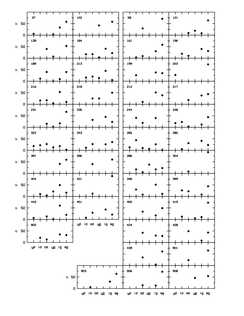
Figure 3: Stellar population found for the 44 objects, 19 in the cluster (left panels) and 25 in the field (right panels). In abcissae we have plotted the 6 population components defined (see text): yd - young dwarfs, id - intermediate dwarfs, od - old dwarfs, yg - young giants, ig - intermediate giants and sg - supergiants.

Forty four synthetic spectra were constructed using the solutions given in Tabs. 5 and 6. Figs. 4 and 5 show these spectra (grey line) superimposed to the observed ones (black line).

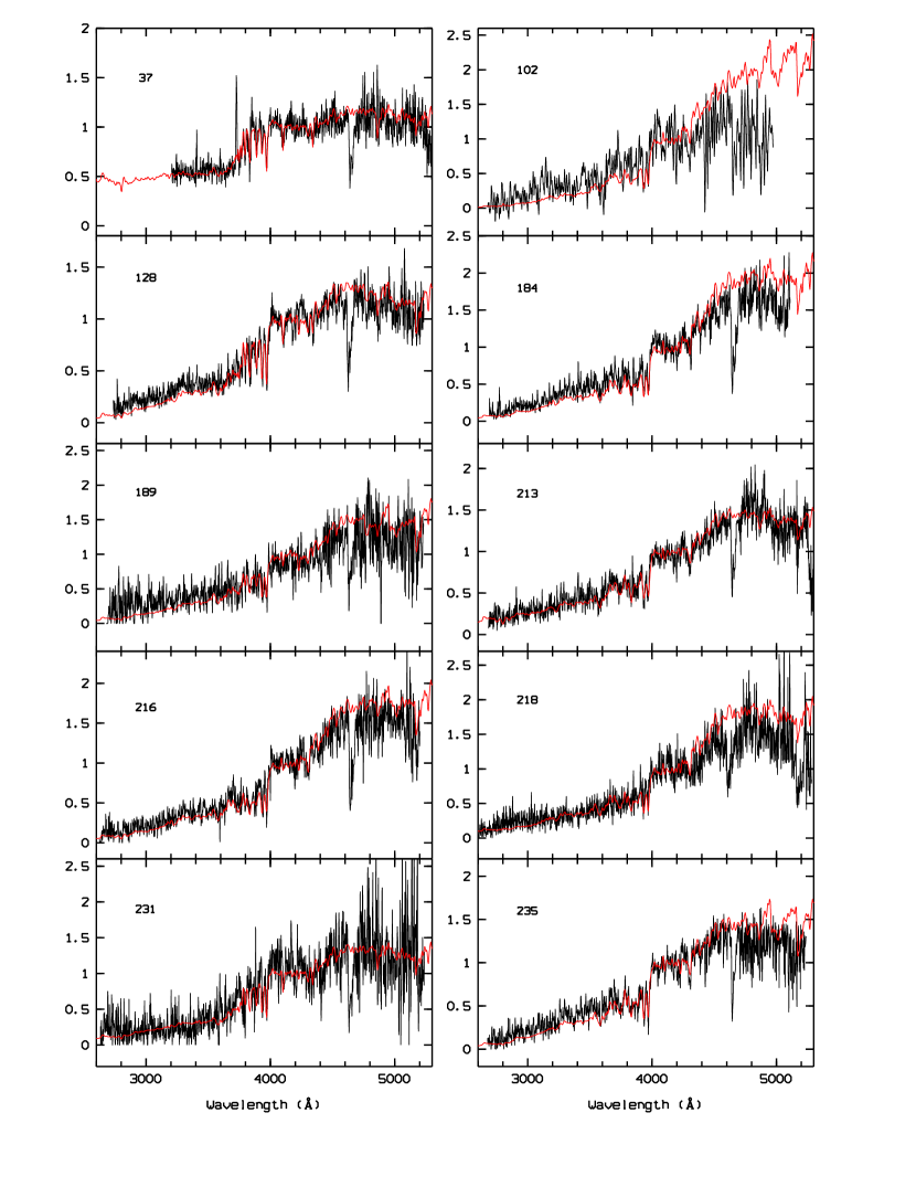
Figure 4: Spectra of the cluster galaxies (black line) in the rest-frame superimposed to the respective synthetic spectra (grey line) computed with the results of the GPG algorithm. All fluxes are relative values.

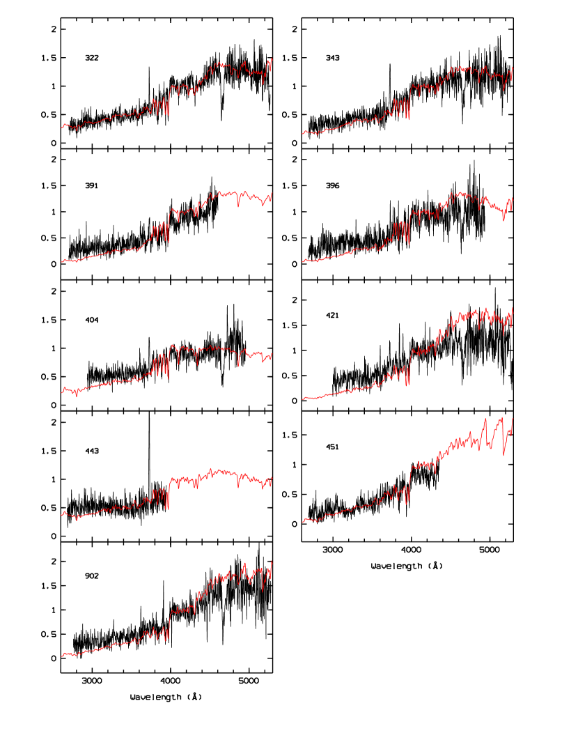
Figure 4: (cont.) Rest-frame and synthetic spectra of the cluster galaxies.

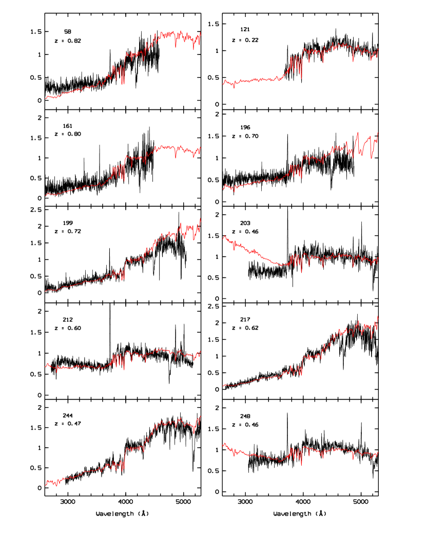
Figure 5: Spectra of the field galaxies (black line) in the rest-frame superimposed to the synthetic ones (grey line) computed with the results of the GPG algorithm. All fluxes are relative values.

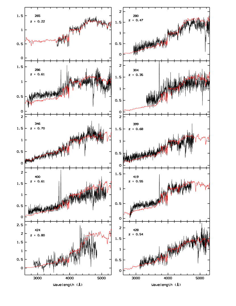
Figure 5: (cont.) Rest-frame and synthetic spectra of the field galaxies.

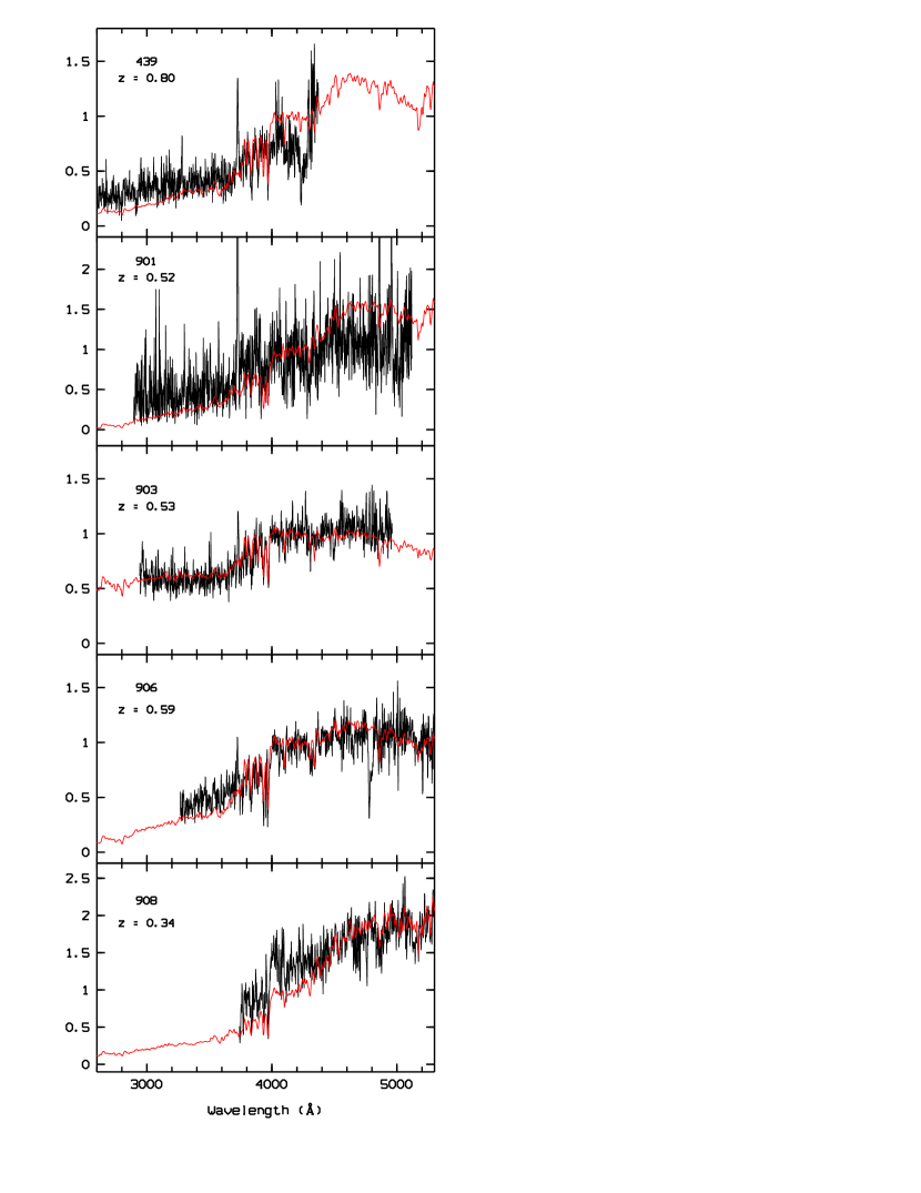
Figure 5: (cont.) Rest-frame and synthetic spectra of the field galaxies.

Looking more closely at the stellar composition in our sample (see Tabs. 5 and 6), we note that three of the population groups we defined are dominant over the other three. These are the supergiant component, the intermediate giant component and the main sequence old one. We will thus base our following analysis on these three classes.

We began by searching for population gradients within the cluster. To do so, we divided the cluster into three different regions according to projected distance to the cluster centre. The galaxies belonging to each concentric region are identified by each of the three symbols in Fig. 6.

Figure 6: Positions of the $19$ cluster member galaxies for which the population synthesis method converged. Each symbol denotes belonging to one of the $3$ different cluster regions, set according to projected distance to the centre (marked by a cross): from diamonds, through triangles up to squares we are moving outwards from the core, through the intermediate regions and to the outskirts (as far out as the cluster virial radius) of projected cluster regions.

Fig 7 shows a gradient trend in the stellar population for two of the three main population classes: old main sequence and supergiants. We have plotted the percentages of these three classes for all galaxies. The data points were also polynomial fitted. Finally, for all galaxies in each group (i.e. centre, intermediate and periphery), we have computed the average of their population components (shown as asterisks in the figure). A population gradient trend is clearly seen: centre galaxies host mainly intermediate giant stars and about the same amount of old main sequence and supergiant stars. As we progress along the cluster towards the outskirts, the old main sequence stars become less abundant while the percentage of supergiants increases. As for the intermediate giant stars no clear gradient is observed, though is seems that their number decreases somewhat towards the periphery of the cluster. We can conclude that galaxies in the cluster core host older stars whereas the stellar populations of galaxies inhabiting the outer cluster regions are dominated rather by young, less evolved stars, i.e. supergiants; this means that star formation is predominantly taking place in the outskirts of the cluster.

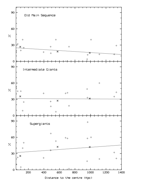
Figure 7: Gradient trends found within the cluster (ranging from the centre through the intermediate region and far out till the outskirts) in terms of the three main population components: old main sequence, intermediate giants and supergiant stars (indicated in percentages). Asterisks denote the mean of the values of each region.

The stellar population of the field galaxies seems to be, in a general way, less evolved that the one found in cluster members. In fact, in terms of ages, young supergiant stars dominate the spectra of field galaxies whereas cluster galaxies host a dominant number of old and intermediate age stars. Fig. 8 shows histograms comparing the three main population components for the field galaxies and for the cluster - as a whole, just the centre and finally its periphery. We took the averages of the values of the population components in each region. We note that the supergiant population is clearly decreasing as we move from the field into the cluster and then to its centre. The old main sequence stars dominate the cluster core with respect to the outskirts and to field galaxies, whereas the intermediate giant population seems to be predominantly present in the cluster (as opposed to what happens in the field).

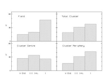
Figure 8: Comparison between the population found: in the field galaxies (upper left); in the cluster as a whole (upper right); in the cluster centre (bottom left) and in the cluster outskirts (bottom right). The standard deviations of the values of these averages vary between 13% and 23%.

6 Analysis on spectral and morphological classes

6.1 Currently used methods

Following the works of Fisher et al. (1998), Balogh et al. (1999), Poggianti et al. (1999), Tran et al. (2003) and references therein we have estimated the percentage of emission line (EL) galaxies and K+A -type galaxies in the cluster and in the field.

These groups of galaxies were defined on the basis of measures of particular spectral features: [OII] in emission and the Balmer series, namely the H$\delta$, H$\gamma$ and H$\beta$ lines when available.

Table 7 shows the bandpass used to measure each feature along with the blue and red -sidebands adopted to determine the local continuum (as in Fisher et al. 1998). This continuum level was estimated by fitting a straight line to the flux in the continuum regions. Equivalent widths were measured using MIDAS. The error due to the uncertainty on where one places the continuum is dominant over all other measurements and statistical uncertainties. For the absorption features we measured, this leads to variations on the EW between $\pm 1$ and $\pm 3$ Å in absolute value, for faint and strong lines, respectively. Whenever the [OII] emission is significant its EW is often underestimated by as much as 9 Å due to this uncertainty. For the weak [OII] lines this variation is always less than 4 Å in absolute value.

Table 7: Line strength index definitions (from Fisher et al. 1998).

Feature	Bandpass	Blue sideband	Red sideband
[OII]	3716.3–3738.3	3696.3–3716.3	3738.3–3758.3
H$\delta$	4083.5–4122.3	4017.0–4057.0	4153.0–4193.0
H$\gamma$	4319.8–4363.5	4242.0–4282.0	4404.0–4444.0
H$\beta$	4847.9–4876.6	4799.0–4839.0	4886.0–4926.0

Galaxies were classified as emission line (EL), normal (N) and post-star forming (K+A) galaxies. Emission line galaxies are those having an equivalent width (EW) of the [OII] emission line equal to or higher than 10 $\AA$. K+A are those presenting both EW([OII]) $<5\AA$ in emission and Balmer absorption features following at least one of the next criteria: EW(H$\delta$) $>5\AA$ or (EW(H$\delta$) + EW(H$\gamma$)) $/2>4\AA$ or (EW(H$\delta$) + EW(H$\gamma$) + EW(H$\beta$)) $/3>4\AA$. Normal galaxies are all the others that do not fit into any of these classes.

Table 8 lists the EWs measured (in Å) as well as the criteria used to define the K+A class, spectral classification, relative position in the cluster and morphological classes given by La Barbera et al. (2003) based on a luminosity profile analysis, performed on VLT/FORS2 images; in what concerns this last entry, we visually identified our galaxies with the map they present (in Fig.9 of their paper) though not all of our galaxies were analysed by La Barbera and collaborators, thus lacking this classification.

Table 8: Classifications for all $54$ galaxies having a redshift measure.

gal id# EW[OII] EW H$\delta$ EW H$\gamma$ EW H$\beta$ EW (H$\delta$+H$\gamma$)/2 EW (H$\delta$+H$\gamma$+H$\beta$)/3 class pos. morph. Cluster: 35 23.4 8.2 1.3 -9.9 4.75 —- EL p — 37 12.3 4.7 4.1 -6.9 4.40 —- EL p — 102 7.0 4.6 2.0 0.0 3.3 —- N it sph 128 1.2 6.0 — 3.6 — —- K+A it disk 184 0.0 1.5 0.0 1.6 0.75 1.0 N it sph 189 0.2 2.1 0.0 2.2 1.05 1.4 N ct sph 213 0.0 0.3 0.5 2.4 0.4 0.9 N ct sph 216 0.0 0.0 0.2 1.1 0.1 0.4 N ct sph 218 0.0 0.0 5.7 2.7 2.8 2.8 N ct sph 231 0.0 3.4 5.5 0.0 4.45 3.0 K+A it disk 235 0.9 1.0 1.1 2.7 1.05 1.6 N ct sph 296 19.7 4.6 2.8 -4.6 3.7 — EL p — 322 5.9 3.9 2.8 2.2 3.35 3.0 N it sph 343 19.0 2.1 0.5 -10.3 1.3 0.9 EL it sph 391 9.4 4.9 6.9 — 5.9 — N it sph 396 9.1 3.7 0.0 0.0 1.8 1.2 N/K+A p disk 404 10.0 3.9 6.2 0.0 5.0 3.4 EL p disk 421 8.7 1.8 2.7 0.0 2.2 1.5 N p sph 443 35.5 — — — — — EL p — 449 28.0 4.9 -1.5 -1.7 — — EL p — 451 0.0 3.1 — — — — N p — 452 34.4 1.9 -4.2 — — — EL p — 902 2.8 2.2 0.9 0.0 1.5 1.0 N p sph Field: 44 — 3.8 1.3 -0.8 2.5 — EL — 58 10.7 6.9 1.8 — 4.4 — EL — 76 32.6 2.6 3.6 -6.4 3.1 — EL — 121 9.4 3.1 2.2 -0.8 2.6 — N — 161 4.9 4.2 7.0 — 5.6 — K+A — 188 69.0 0.0 4.5 -24.0 — — EL — 196 17.1 4.8 2.9 -13.2 3.8 — EL disk 199 9.2 0.6 0.0 3.6 0.3 1.4 N sph 203 23.0 6.0 3.7 -2.4 4.8 — EL — 212 31.5 4.9 2.0 -7.5 2.3 — EL — 217 0.0 0.0 0.1 1.1 0.05 0.4 N sph 244 2.0 0.0 1.6 3.7 0.8 1.8 N — 245 10.8 7.9 4.7 — 6.3 — EL — 248 17.7 1.8 0.3 -1.1 1.0 — EL — 265 0.0 2.3 2.4 2.5 2.35 2.4 N — 266 14.0 4.9 5.5 — 5.2 — EL — 280 0.0 1.5 0.0 3.3 0.75 1.6 N — 286 7.8 6.5 — 2.6 — — N disk 304 25.4 6.9 0.0 -4.9 3.0 — EL — 346 0.0 1.6 0.9 2.8 1.2 1.8 N sph 399 5.4 — — — — — N/K+A disk 400 27.4 5.1 2.0 -0.5 3.6 — EL sph 419 12.7 2.8 4.7 — 3.8 — EL sph 424 0.0 -2.7 0.0 — — — N sph 428 3.1 0.7 4.3 1.3 2.5 2.1 N sph 439 17.9 4.4 2.5 — 3.4 — EL disk 901 53.6 10.6 0.7 -13.0 5.6 — EL sph 903 7.8 3.3 3.5 -0.2 3.4 — N sph 906 5.6 3.9 — — — — N — 907 30.7 2.9 0.0 -9.2 1.4 — EL sph 908 0.0 3.0 2.2 3.7 2.6 3.0 N/K+A —

Notes: All EW are given in Å; Column “class” gives the spectral classification. For three of the objects (#396, #399, #908), since the two methods described (see sections 6.1 and 6.2), do not give the same result, we display both of them. Column “pos.” indicates the relative position of each cluster galaxy within the cluster as in Fig. 6 (“ct” stands for centre or core; “it” denotes the intermediate region and “p” identifies peripheral galaxies. Finally, column “morph.” lists the morphological classification attributed by La Barbera et al. (2003): “sph” (for spheroidal galaxies) and “disks”.

We note that our spectra were not corrected from telluric absorption so, in some cases, the equivalent widths of the Balmer lines were contaminated by this effect. Whenever this happened, the respective line was not considered for our criteria (no entry in Table 8 is given).

Table 9 sums up the main results, in terms of percentages, regarding the fractions of the different spectral-type galaxies within the cluster and in the field.

Table 9: Number and percentages of the different galaxy classes found in the cluster (as a whole and in different regions) and in the field.

Cluster	EL	K+A	N
all	8 (35%)	2 (9%)	13 (56%)
centre	0	0	5 (100%)
intermediate	1 (14%)	2 (29%)	4 (57%)
periphery	7 (64%)	0	4 (36%)
Field	16 (52%)	1 (3%)	14 (45%)

With regard to the cluster, one can definitely observe some trends: we find larger percentages of normal galaxies as we move from the outskirts to the centre, whereas the number of emission line galaxies decreases towards the central regions. This agrees with previous results derived for example from the ENACS survey for lower-z clusters, where emission line galaxies are found to be more abundant towards the outskirts of clusters (Biviano et al. 1997). The K+A galaxies inhabit the intermediate cluster region. Such overall trends have been also identified in the CNOC1 sample of 15 clusters by Ellingson et al. (2001) using a principal component analysis method.

Looking more closely at the K+A class, and having calculated its relative frequency and Possionian error in the same way as other authors, we can compare our results (9% $\pm$ 6% of this type) directly to theirs. Balogh et al. (1999) find an average of 4.4% $\pm$ 0.7% K+A galaxies in their sample of 15 clusters at 0.18 $<$ z $<$ 0.55, using selection criteria similar to ours, and the same measuring method (we note that Tran et al. 2003 argue that these fractions should probably be somewhat higher though).

Dressler et al. (1999) report a mean value of $\sim$ 20% of k+a and a+k (i.e. moderate and strong Balmer absorption galaxies without emission) for a sample of 10 clusters ranging from z=0.37 to z=0.56. However, their selection criterium differs from the usually adopted one in the sense that every object with an EW of the H$\delta$ line larger than 3 Å is considered in this class, probably justifying to some extent their higher percentages.

For 3 clusters at redshifts 0.33, 0.58 and 0.83, Tran et al. (2003) determine a fraction of E+A galaxies of 9% $\pm$ 2%, 7% $\pm$ 2% and 16% $\pm$ 3% respectively, using exactly the same method we followed here.

It is hard to draw any definite conclusion when comparing our results to these (and other) works. Even if the method for measuring spectral features is the same, the magnitude limits, spectroscopic (in)completeness, quality of the spectra, spatial coverage of the clusters and possibly other factors are bound to play a role, and the contribution of such parameters has not yet been investigated.

6.2 An alternative method for identifying post-star forming galaxies

The method we have just used to measure the EW of the lines, though being the one used by other authors and thus allowing direct comparisons to be made, does not seem to us as being a reliable one as the continua used for the measures are not well defined in many cases. The EW of the features are normally underestimated, as the continuum traced is too low (or overestimated in case of a too high local continuum, which happens in fewer cases).

The criteria that are used intend to find the galaxies with strong absorption Balmer lines, which appear mainly in A-type stars. In our work, since we performed stellar population synthesis for almost all galaxies observed, both in the cluster and in the field, we have direct access to this information. So, it seems much more natural to search for these stellar types through the synthesis. We have thus viewed several stellar spectra and decided, by means of the relative strength between the CaII H+K, H$\delta$, H$\gamma$ and the G-band, in which stellar types the Balmer lines are important features, i.e. with EW $\geq 6-7$ Å. We concluded that they appear quite intensely not only in A-type stars but also for some B and F types: in fact, stars from B5 to F2 spectral types show important absorption of the Balmer lines. We have then searched in the solutions of the synthesis for galaxies presenting these types of stars in a large enough percentage so that these lines are still strong in the final synthetic spectra (see Figs. 4 and 5). We found that this is the case for percentages equal to or higher than 30%, so we established this value as our threshold. Having identified the galaxies that pass this criterion we then eliminated those with significant emission in their spectra.

This led us to a final sample of three K+A galaxies in the cluster and three in the field. Of these, three had already been found by applying the criteria of the other authors (#128 and #231 within the cluster, #161 in the field) and 3 are new ones (#396 in the cluster peripheral region, #399 and #908 in the field).

We are convinced that the criteria generally used to identify these galaxies are not good, leading to an underestimate of the absolute number of existing K+A galaxies. We believe that this is mainly due to the way of measuring the Balmer lines EWs which, in many cases, underestimates the line strengths. Some authors (Dressler et al. 1999) had already noticed this problem and had pointed to the fact that in some cases “strange continua” lead to “strange measures” of EW, these appearing in emission (negative values of EW) when in fact the lines are well seen in absorption. We subscribe to this view and add that, due to this problem, K+A galaxies are often lost.

Comparing our results of K+A percentages obtained with the two methods (i.e. through means of the population synthesis and by the standard criteria), within the sample of galaxies that we observed in cluster CL 0048-2942, 13% are K+A galaxies (contrarily to the 9% previously estimated), whereas the field has 10% of these galaxies (instead of 3%).

Table 10 gives the new classification results when applying the new method.

Table 10: Same as Table 9 but using the new classification method, based on the stellar population synthesis results.

Cluster	EL	K+A	N
all	8 (35%)	3 (13%)	12 (52%)
centre	0	0	5 (100%)
intermediate	1 (14%)	2 (29%)	4 (57%)
periphery	7 (64%)	1 (9%)	3 (27%)
Field	16 (52%)	3 (10%)	12 (38%)

Regarding morphology, and going back to Table 8, we find that all galaxies in the centre (N galaxies) are spheroids; in the intermediate region, the two K+A galaxies are disks, the EL is a spheroid, and the remaining ones (N galaxies) are all spheroids. As for the periphery, morphological classification is available for four galaxies only: two are spheroids (N galaxies) and two are disks (one EL and one K+A). So, in terms of a morphological gradient, spheroids are more abundant in the centre and their number decreases as one moves to the outskirts of the cluster, being replaced by disk galaxies. Quantitatively, we find 100% of spheroids in the centre, 71% of spheroids and 29% of disk galaxies in the intermediate region, while the outer region presents 50% of disk galaxies and 50% of spheroids even though this last result must be taken with caution since we lack the morphological classifications for six of the galaxies. However, La Barbera et al. (2003), with a different cluster sampling, also find a greater central concentration of spheroids whereas disks are predominantly located towards the outskirts of the cluster, in regions of lower galactic density.

As for field, and contrarily to what happens in the cluster, N galaxies are much less frequent, being outnumbered by EL ones. This kind of result has been observed long ago (see e.g. Balogh et al. 1997 and references therein) and remains evident in the latest surveys (e.g. Goto et al. 2003).

For the EL field galaxies, their EW([OII]) reaches higher values (up to twice as much) than in their cluster counterparts leading us to believe that star formation is more intense in the field - or, rather, suppressed within the cluster. Besides, and as far as we have probed the cluster periphery (where the probability of observing infall galaxies is higher), no enhancement of the star formation is detected in cluster members. Evidence for lower star formation rates within the virial radius for intermediate to high -redshift clusters relatively to the coeval field had already been reported by e.g. Balogh et al. (1997, 1998, 1999), Ellingson et al. (2001), Postman et al. (2001), Kodama & Bower (2001), Lewis et al. (2002), Gómez et al. (2003). Regarding our work, though, two caveats need to be taken into account before drawing any conclusions: (1) we do have limited spectroscopic coverage, which may have caused us to miss a fraction of star forming galaxies - farthest away from the cluster core - that equal or even supersede the coeval field counterparts (in number and/or in star forming activity); (2) our field galaxy sample is not coeval with the cluster galaxies, hampering direct comparisons. However, we note that it is equally composed of foreground and background galaxies: $15$ and $16$, respectively; in each of these two groups, $6$ and $11$ galaxies are ELs and the average EWs of the [OII] emission are $16.8$ Å and $30.2$ Å, respectively. Instead, the $8$ cluster ELs produce an average EW of the [OII] emission line of $22.8$ Å. The only thing one can say from these figures is that for those galaxies within the virial radius of CL 0048-2942 undergoing star formation, we would expect their activity to be equal to or lower than the coeval field galaxies. Whether the fraction of EL galaxies is higher or lower than in the coeval field cannot be ascertained from our observations.

Furthermore, it is interesting to note that all the K+A galaxies we identified in our samples (cluster and field) having a morphological classification by La Barbera et al. (2003) (4 in a total of 6) are disk galaxies. This agrees with previous findings that the majority of these systems seem to be disks (Kelson et al. 200, Tran et al. 2003 and references within these papers).

One last consideration concerning the results presented in this section and in the previous one: we are aware that projection effects may have an influence on our results, but our limited amount of data on cluster members prevents us from making any correction; the conclusions we reached should thus be taken rather as indications only. However, we recall that de-projecting distances is heavily dependent on the cluster density profile one assumes - a source of uncertainties that are hard to quantify -, and is expected not to change results qualitatively (Ellingson et al. 2001). Still, a larger amount of redshifts would enable us to perform a complementary line-of-sight approach, thus giving us a full and desirable three-dimensional view of the galaxy population properties of CL 0048-2942.

7 Colours

The galaxy population gradient revealed by our stellar population synthesis analysis (and presented in section 5.3) is confirmed by the colours of the cluster members, once we distribute them into the same classes as before (centre, intermediate and periphery), which can be translated into cluster-centric projected distances (see Fig. 9). Central galaxies have in average the colour of the red sequence, R$-$I$=1.12$ magnitudes, that signals the cluster presence in a colour-magnitude plot, as determined by Andreon et al. (2004). Then, as one moves away from the centre of the cluster, there is a clear trend of blueing of the stellar population. The change of galaxy colour as a function of radius has been observed since the works of Butcher & Oemler (1978, 1984) within the same physical region we are probing in CL 0048-2942 and even till further out (Kodama & Bower 2001; Pimbblet et al. 2002). We have also plotted the stellar population parameters in terms of the 3 main components (old main sequence, intermediate giants and supergiant stars) versus colour and distance to the cluster centre (see Figure 10). Note the trends in the stellar populations as we move from the centre towards the outskirts of the cluster. Regarding colour and stellar populations one can see, by inspection of Figure 10, that in fact, supergiants are the stellar class more abundant in the bluer colours whereas giants and main sequence stars together are more important for redder ones.

Figure 9: R-I colour as a function of cluster-centric projected distance for all cluster galaxies having reliable photometry. For these objects the mean value of the error in the R-I colour is $\sim$ 0.03 mag. Open symbols are the same as in Fig. 6, indicating the cluster-centric distance class in which a galaxy is considered. Filled symbols give, at mean distance for each class, the mean colour of that class (the “error bar” indicates the dispersion of the values used to compute the average). Smaller dots refer to field galaxies.

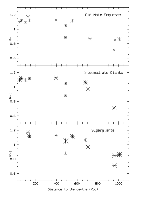
Figure 10: Colours versus distance to the centre of the cluster. The symbols sizes are proportional to the percentages of the 3 stellar population components indicated in each panel.

CL 0048-2942 has a fraction of blue galaxies f${}_{b}=0.29\pm 0.05$ (Andreon et al. 2004; though see La Barbera et al. 2003 for a different estimate). Such a value is compatible with the extrapolation to $z\sim 0.6$ of the Butcher & Oemler (1984) results, and so could be providing an indication of a significant content of blue galaxies. However, a rigorous analysis on the computation of error bars presented also in Andreon et al. (2004), does not allow to rule out a constant blue fraction with redshift for the whole Butcher & Oemler sample including CL 0048-2942. Apart from demonstrating the uncertainties that still prevail in establishing the Butcher-Oemler effect as a fact, those results show that the population of CL 0048-2942 seems to be just as blue as one would expect from the age of the galaxies at $z\sim 0.64$.

8 Summary

We studied a field centered on cluster CL0048-2942, measuring redshifts for 54 objects, 23 of them belonging to the cluster with redshift of around 0.64. The line-of-sight velocity dispersion of CL0048-2942, based on this sample, is $680$ $\pm$ 140 km/s.

Our analysis have unveiled some interesting radial trends in the galaxy population, namely the existence of (1) a stellar populations gradient, (2) a spectral classes gradient and (3) a colour gradient.

Our stellar populations synthesis method revealed that centre cluster galaxies host mainly intermediate and old stars; such a population gradually seems to change towards the outskirts of the cluster (as far out as its virial radius, approximately), where supergiants dominate the spectra of the galaxies, denoting a higher rate of star formation in this region. This trend is followed by the colours of the galaxies: redder in the cluster inner regions and bluer at larger radial distances.

Field galaxies, analysed with the same method, are found to be predominantly made of less evolved stars, namely supergiants, with smaller components of main sequence and giant stars.

The stellar populations, both for cluster and for field galaxies, are mainly poor in dust content.

In what concerns spectral classes, we used a new method, based on the stellar population synthesis results, that takes into account all possible absorption features in the spectrum and thus makes optimal use of the data. We thus find that emission-line galaxies are present mainly in the field and in the outskirts of the cluster whereas normal galaxies are concentrated in the centre of the cluster. Concerning K+A galaxies, 3 were found in the cluster (in the intermediate and peripheral regions) and 3 in the field. Comparisons were attempted with the estimates provided by several authors on the K+A content of different redshift clusters. However, poor statistics and the unknown contribution of numerous involved parameters, such as incompleteness, magnitude limit, quality of the spectra, etc., do not permit to draw any definite conclusions.

We correlated our cluster data with morphological information produced by La Barbera et al. (2003), concluding that 100cluster galaxies are spheroids, while there are 71disk galaxies in the intermediate region. The outer region presents 50of the galaxies in this region.

To conclude, we believe the trends reported in this paper to be real: we have no reason to expect our spectroscopic sampling to suffer from any selection bias, so the results that we have obtained here should provide a good indication of the whole picture. The radial gradients that we observe could then be tracing a “radial evolution” of the cluster members and tempt us into inferring some implications on environmentally-driven changes, probably in the sequence of infall episodes. On the other hand, it could simply reflect the morphology-density relation (Dressler 1980). Choosing between the two scenarios for CL 0048-2942 would require morphological classification for all our sampled galaxies as well as for a field sample observed in the same redshift range, and a larger spatial coverage with complete spectroscopy.

A growing feeling, however, is that local density does seem to play a key role in spectral characteristics that reveal spectral class transformations, which can be accompanied - though in different, longer, time scales - by morphological ones. The limiting surface density that marks the separation between field-type and cluster-like galaxies, at least in terms of star formation, should be around 1 Mpc^-2, which generally is attained around the virial radius (see Bower & Balogh 2004 and references therein), our limit of spatial coverage for CL 0048-2942.

It would be interesting to push our analyses further, complementing our results with local density measures (as performed by e.g. Kodama et al. 2001, Lewis et al. 2002, Pimbblet et al. 2002, Gómez et al. 2003, Balogh et al. 2004, Kauffmann et al. 2004) and trying to understand whether these accompany the gradients we detected. Given the low numbers we are dealing with in this paper, it wouldn’t be sensible to try and measure a density so as to compare with the works referenced above. This work is thus a future prospect for CL 0048-2942.

- (1) Abell G.O. 1958, ApJS 3, 211
- (2) Andreon S., Lobo C., Iovino A. 2004, MNRAS 349, 889
- (3) Arnaud M., Evrard A.E. 1999, MNRAS 305, 631
- (4) Balogh M.L., Morris S.L., Yee H.K.C., Carlberg R.G., Ellingson E. 1997, ApJ 488, L75
- (5) Balogh M.L., Schade D., Morris S.L. et al. 1998, ApJ 504, L75
- (6) Balogh M.L., Morris S.L., Yee H.K.C., Carlberg R.G., Ellingson E. 1999, ApJ 527, 54
- (7) Balogh M., Bower R.G., Smail I. et al. 2002, MNRAS 337, 256
- (8) Balogh M., Eke V., Miller C. et al. 2004, MNRAS 348, 1355
- (9) Blanton E.L., Gregg M.D., Helfand D.J. et al. 2003, AJ 125, 1635
- (10) Benoist C., da Costa L., Jørgensen H.E. 2002, A&A 394, 1
- (11) Bertin E., Arnouts S., 1996, A&AS 117, 393
- (12) Best P.N., Lehnert M.D., Miley G.K., Röttgering H.J.A. 2003, MNRAS 343, 1
- (13) Biviano A., Katgert P., Mazure A. et al. 1997, A&A 321, 84
- (14) Bower R.G., Balogh M.L. 2004, in “Clusters of Galaxies: Probes of Cosmological Structure and Galaxy Evolution”, eds. J.S. Mulchaey, A. Dressler, and A. Oemler, p. 326
- (15) Bressan A., Fagotto F., Bertelli G., Chiosi C. 1993, A&ASS 100, 647
- (16) Brown M.J.I., Webster R.L., Boyle B.J. 2001, AJ 121, 2381
- (17) Butcher H., Oemler A. 1978, ApJ 219, 18
- (18) Butcher H. & Oemler A. 1984, ApJ 285, 426
- (19) Cardelli J.A., Clayton G.C., Mathis J.S. 1989, ApJ 345, 245
- (20) Condon J.J., Cotton W.D., Greisen E.W. et al. 1998, AJ 115, 1693
- (21) Couch W.J., Sharples, R. M. 1987, MNRAS 229, 423
- (22) Della Ceca R., Scaramella R., Gioia I.M. et al. 2000, A&A, 353, 498
- (23) Deltorn J.-M., Le Fèvre O., Crampton D., Dickinson M. 1997 ApJ 483, L21
- (24) Dressler A., 1980, ApJ 236, 351
- (25) Dressler A., Gunn J.E. 1983, ApJ 270, 7
- (26) Dressler A., Smail I., Poggianti B.M. 1999, ApJS 122, 51
- (27) Dressler A. 2004, in “Clusters of Galaxies: Probes of Cosmological Structure and Galaxy Evolution”, eds. J.S. Mulchaey, A. Dressler, and A. Oemler, p. 207
- (28) Donahue M., Voit G.M., Gioia, I. et al. 1998, ApJ, 502, 550
- (29) Eales S.A. 1985, MNRAS 214, 27
- (30) Ebeling H., Jones L.R., Perlman E. et al. 2000, ApJ 534, 133
- (31) Ebeling H., Jones L.R., Fairley B.W. et al. 2001, ApJ 548, L23
- (32) Ellingson E., Lin H., Yee H.K.C., Carlberg R.G. 2001, ApJ 547, 609
- (33) Fisher D., Fabricant D., Franx M., van Dokkum P. 1998, ApJ 498, 195
- (34) Gómez P.L., Nichol R.C., Miller C.J. et al. 2003, ApJ 584, 210
- (35) Goto T., Nichol R.C., Okamura S. et al. 2003, PASJ 55, 771
- (36) Goto T., Yagi M., Tanaka M., Okamura S. 2004, MNRAS 348, 515
- (37) Hartwick F.D.A. 2004, ApJ 603, 108
- (38) Howarth I.D., 1983, MNRAS 203, 301
- (39) Katgert P., Mazure A., Perea J. et al. 1996, A&A 310, 8
- (40) Kauffmann G. 1995, MNRAS 274, 161
- (41) Kauffmann G., White S.D.M., Heckman T.M. et al. 2004, MNRAS submitted or astro-ph/0402030
- (42) Kelson D.D., Illingworth G.D., van Dokkum P.G., Franx M. 2000, ApJ 531, 184
- (43) Kennicutt R.C. 1983, AJ 88, 483
- (44) Kodama T., Bower R.G. 2001, MNRAS 321, 18
- (45) Kodama T., Smail I., Nakata F., Okamura S, Bower R.G. 2001, ApJ 562, L9
- (46) La Barbera F., Merluzzi P., Iovino A. et al. 2003, A&A 399, 899
- (47) Landolt A.U. 1992, AJ 104, 340
- (48) Lewis I., Balogh M., De Propris R. et al. 2002, MNRAS 334, 673
- (49) Lilly S.J., Le Fèvre O., Hammer F., Crampton D. 1996, ApJ 460, L1
- (50) Lima Neto G.B., Capelato H.V., Sodré L. Jr, Proust D. 2003, A&A 398, 31
- (51) Lobo C., Iovino A., Lazzati D., Chincarini G., 2000, A&A 360, 896
- (52) Lubin L.M., Postman M.; Oke J.B. et al. 1998, AJ 116, 584
- (53) Lubin L.M., Oke J.B., Postman M. 2002, AJ 124, 1905
- (54) Lubin L.M., Mulchaey J.S., Postman M. 2004, ApJ 601, L9
- (55) Luppino G.A., Gioia I.M. 1995, ApJ, 445, L77
- (56) Madau P., Ferguson H.C., Dickinson M.E. et al. 1996, MNRAS 283, 1388
- (57) Madau P., Pozzetti L., Dickinson M. 1998, ApJ 498, 106
- (58) Nonino M., Bertin E., da Costa L. et al. 1999, A&AS 137, 51
- (59) Oemler A.,Jr. 1974 ApJ 194, 10
- (60) Pelat D., 1997, MNRAS 284, 365
- (61) Pickles A.J., 1998, PASP 110, 863
- (62) Pimbblet K.A., Smail I., Kodama T. et al. 2002, MNRAS 331, 333
- (63) Poggianti B.M., Smail I., Dressler A. et al. 1999, ApJ 518, 576
- (64) Postman M., Lubin L.M., Oke J.B. 1998, AJ 116, 560
- (65) Postman M., Lubin L.M., Oke J.B. 2001, AJ 122, 1125
- (66) Quintero A.D., Hogg D.W., Blanton M.R. et al. 2004, ApJ 602, 190
- (67) Ramella M., Biviano A., Boschin W. et al. 2000, A&A 360, 861
- (68) Rosati P., Stanford S.A., Eisenhardt P.R. et al. 1999, AJ 118, 76
- (69) Schlegel D.J., Finkbeiner D.P., & Davis M. 1998, ApJ, 500, 525
- (70) Smith G.P., Treu T., Ellis R.S., Moran S.M., Dressler A. 2004, ApJ submitted or astro-ph/0403455
- (71) Tonry J., Davis M., 1979, AJ 84, 1511
- (72) Tran K.-V.H., Franx M., Illingworth G. et al. 2003, ApJ 599, 865
- (73) Tran K.-V.H., Franx M., Illingworth G. et al. 2004, ApJ accepted or astro-ph/0403484
- (74) Valtchanov I., Pierre M., Willis J. et al., 2003, A&A submitted or astro-ph/0305192
- (75) van Dokkum P.G., Franx M., Kelson D.D., Illingworth G.D. 1998, ApJ 504, L17
- (76) van Dokkum P.G., Franx M., Fabricant D., Kelson D.D., Illingworth G.D. 1999, ApJ 520, L95
- (77) Wittman D., Margoniner V.E., Tyson J.A. et al. 2003, ApJ 597, 218
- (78) Wu X.-P., Fang L.-Z., Xu W. 1998, A&A 338, 813
- (79) Wu X.-P., Xue Y.J., Fang L.-Z., 1999, ApJ 524, 22
- (80) Yates M.G., Miller L., Peacock J.A. 1989, MNRAS 240, 129
- (81) Yee H.K.C., Ellingson E., Carlberg R.G. 1996, ApJS 102, 269
- (82) Yee H.K.C., López-Cruz O. 1999, AJ 117, 1985
- (83) Yee H.K.C., Ellingson E. 2003, ApJ 585, 215