An Optical Catalog of the Chandra Large Area Synoptic X-ray Survey Sources

Abstract

We present photometric and spectroscopic observations of the X-ray sources detected in the wide-area, moderately deep Chandra Large Area Synoptic X-ray Survey of the Lockman Hole-Northwest field. We have $B$, $V$, $R$, $I$, and $z^{\prime}$ photometry for 521 (99%) of the 525 sources in the X-ray catalog and spectroscopic redshifts for 271 (52%), including 20 stars. We do not find evidence for redshift groupings of the X-ray sources, like those found in the Chandra Deep Field surveys, because of the larger solid angle covered by this survey. We separate the X-ray sources by optical spectral type and examine the colors, apparent and absolute magnitudes, and redshift distributions for the broad-line and non-broad-line active galactic nuclei. Combining our wide-area survey with other Chandra and XMM-Newton hard X-ray surveys, we find a definite lack of luminous, high accretion rate sources at $z<1$, consistent with previous observations that showed that supermassive black hole growth is dominated at low redshifts by sources with low accretion rates.

1 Introduction

The $2-8$ keV X-ray extragalactic background light is dominated by sources with fluxes around $f_{2-8~{}{\rm keV}}\simeq 10^{-14}$ ergs cm^-2 s^-1 (Cowie et al. 2002). To obtain a more complete picture of the history of X-ray production in active galactic nuclei (AGNs), these sources, which have surface densities of only a few hundred deg^-2, need to be studied in more detail. Since the Chandra Deep Field (CDF) surveys (CDF-N, Brandt et al. 2001 and Alexander et al. 2003; CDF-S, Giacconi et al. 2002) cover too little solid angle (0.12 and 0.11 deg², respectively) to provide a large sample of such sources, we have undertaken a wide-area (0.4 deg²), contiguous Chandra survey of the Lockman Hole – Northwest field. The X-ray properties of the sources in our survey — called the Chandra Large Area Synoptic X-ray Survey, or CLASXS — are described in the companion paper by Yang et al. (2004); hereafter, Y04.

We designed CLASXS to sample a large, contiguous solid angle, while remaining sensitive enough to measure sources $2-3$ times fainter than the observed break in the $2-8$ keV log $N-$log $S$ distribution (e.g., Mushotzky et al. 2000; Campana et al. 2001; Brandt et al. 2001; Hasinger et al. 2001; Baldi et al. 2002; Rosati et al. 2002; Stern et al. 2002; Alexander et al. 2003; Harrison et al. 2003; Kim et al. 2004; Wang et al. 2004). We chose a survey size of about 0.4 deg² based on ASCA observations, which show a 6% rms variance for hard X-ray intensities on a scale of $0.5$ deg² (Kushino et al. 2002). This variance is believed to be responsible for the discrepancies in the number counts among the ultradeep Chandra surveys (Cowie et al. 2002). With CLASXS, we are able to examine the large scale structure of the X-ray sources (Yang et al. 2003), something that cannot be done by combining random, non-contiguous Chandra pointings. CLASXS is the essential step between the ultradeep, narrow Chandra surveys and wide-field, shallow surveys, such as those obtained by ROSAT and ASCA.

In this paper, we present photometric and spectroscopic data of the optical counterparts to the CLASXS sources. We briefly describe the X-ray observations in § 2. (A full discussion may be found in Y04.) We discuss our photometric observations in § 3, our spectroscopic data in § 4, and the photometric and spectroscopic properties of the CLASXS sources in §§ 5 and 6, respectively. In § 7, we present the colors and luminosities of the CLASXS sources. In §§ 8 and 9, respectively, we discuss our results and summarize our main conclusions. We use J2000 coordinates and the cosmological parameters $H_{0}=65$ km s^-1 Mpc^-1, $\Omega_{M}=\text@frac{1}{3}$, and $\Omega_{\Lambda}=\text@frac{2}{3}$.

2 X-ray Imaging

To minimize the effects of Galactic attenuation, we chose to position our CLASXS survey in the Lockman Hole (specifically, the Lockman Hole - Northwest, one of two Infrared Space Observatory [ISO] fields observed by Kawara et al. 2004), which has the lowest integrated H I Galactic column density in the sky (N${}_{H}=5.7\times 10^{19}$ cm^-2; Lockman et al. 1986). Kappes, Kerp, & Richter (2003) find an additional ionized hydrogen component that comprises $20-50\%$ of the attenuating material; however, limitations on their data prevent a calculation of the precise ionization fraction. Regardless, the total hydrogen content is too low to significantly affect the X-ray properties. For reference, we note that our field is located $\sim 2.5\deg$ northwest of the ROSAT Lockman Hole field (Hasinger et al. 1998), which was also observed by ASCA (Ishisaki et al. 2001), BeppoSAX (Giommi, Perri, & Fiore 2000), Chandra (Lehmann et al. 2002), and XMM-Newton (Hasinger et al. 2001).

CLASXS consists of nine contiguous Chandra ACIS-I exposures approximately arranged in a $3\times 3$ grid centered at $(\alpha,\delta)_{J2000}=$ (10:34:02.1, +57:46:25.0). The aim points are separated by about $10\arcmin$. The central field has a longer integration (70 ks) than the surrounding eight 40 ks fields. The total field coverage is $0.36$ deg², with 70 ks aim point flux limits (Y04) of $5\times 10^{-16}$ ergs cm^-2 s^-1  (soft; $0.4-2.0$ keV) and $3\times 10^{-15}$ ergs cm^-2 s^-1  (hard; $2-8$ keV). We have detected 525 independent X-ray sources in at least one of the three X-ray bands. In Y04, the X-ray fluxes for the CLASXS sources were calculated from the observed X-ray counts using individual power-law indicies that were based on the ratio of the hard-to-soft X-ray counts (i.e. hardness ratios). Here we have converted the $0.4-2$ keV Y04 fluxes into $0.5-2.0$ keV fluxes using a power-law spectral energy distribution with a photon index of $\Gamma=1.8$ and a column density of N${}_{H}=5.7\times 10^{19}$ cm^-2. If a source is not detected in all of the X-ray bands, then an upper limit for the flux in any undetected X-ray band is calculated by measuring the flux at the source position (as measured in the detected band) using a circular aperture and removing the local background signal. If the local background flux is larger than the flux measured at the source position, then the background flux is used as an upper limit for the source. Additional information regarding the CLASXS X-ray catalog, including reduction and analysis procedures, can be found in Y04.

All 525 CLASXS X-ray sources from Y04 are listed in Table 1 in the Appendix, which also gives the optical magnitudes and spectroscopic redshifts, when available (see §§ 3 and 4).

3 Optical Imaging

We obtained deep broadband Johnson B and V, Cousins R and I, and Sloan $z^{\prime}$ observations reaching $2\sigma$ AB magnitudes of $27.8$, $27.5$, $27.9$, $26.4$, and $26.2$, respectively, with Suprime-Cam (Miyazaki et al. 2002) on the Subaru 8.2 m telescope. Using the Canada-France-Hawaii Telescope (CFHT) with the CFH12K camera, we obtained wider field images in broadband Johnson B, Cousins R, and CFHT $z^{\prime}$ reaching $2\sigma$ AB magnitudes of $27.6$, $27.9$, and $26.3$. Table 2 summarizes the telescopes, dates of the observations, and the integration times. Table 3 summarizes the average seeing, $2\sigma$ limits, and areas of each image. The images and the optical source catalog are presented in Capak et al. (2004b), in which a more extensive discussion of the observations and reductions can be found. We briefly summarize the Suprime-Cam and CFH12K observations and reductions in the Appendix.

3.1 Optical Source Detection

We performed source detection on the R-band image using the program SExtractor (Bertin & Arnouts 1996). To improve faint source detection and minimize sky noise, the image was smoothed using a $2\arcsec$ Gaussian kernel. The detection threshold was set to be eight contiguous pixels with counts at least $2~{}\sigma$ above the sky background. We measured the optical magnitude of each source with the IDL routine APER, using a 3″ diameter aperture centered on the optical counterpart, if detected, or on the X-ray position if not. The magnitudes of bright sources that are significantly larger than the 3″ aperture are underestimated, as are $R<20$ sources, which are typically saturated in our images.

Table 1 in the Appendix gives the optical properties of the CLASXS X-ray sources. The CLASXS source number (from Y04) is given in column (1). The positions for the detected optical counterparts are given in columns (5)-(6). The aperture-corrected $B$, $V$, $R$, $I$, and $z^{\prime}$ magnitudes are given in columns (9)-(13). Column (14) gives the measured redshifts of identified sources. In this column, we labeled spectroscopically identified stars “star”. If we spectroscopically observed a source but did not identify it, then we labeled the source “obs”.

The aperture correction was calculated by examining the curve of growth for isolated, moderately bright ($R=20-26$) sources. The 3″ aperture corrections for the Subaru (CFHT) images are $-0.17$ ($-0.30$), $-0.22$, $-0.11$ ($-0.15$), $-0.33$, and $-0.13$ ($-0.22$), for the B, V, R, I, and $z^{\prime}$ bands, respectively. Sources that fall outside of the field of view of a given filter are left blank. If a source falls within the field of view but is not detected, then it is assigned the $2~{}\sigma$ magnitude limit for that filter and is considered an upper limit.

3.2 Optical Counterpart Identifications of the CLASXS X-ray Sources

Chandra’s cylindrical mirrors were designed to be the smoothest mirrors ever constructed in an effort to obtain the highest resolution X-ray images ever ($\sim 0.5\arcsec$ at the aim point), and thus the most accurate positions for the sources. This unprecedented X-ray positional accuracy allows the secure identification of counterparts at other wavelengths. The cylindrical mirror design, which is required for the grazing incidence optics needed to focus X-rays, introduces an aberration that increases the point spread function (PSF) of an image with an off-axis angle. For example, Chandra’s PSF at an off-axis angle of $6\arcmin$ ($12\arcmin$) from the aim point is $\sim 2.5\arcsec$ ($\sim 9\arcsec$). This increasing X-ray PSF size with off-axis angle makes it difficult to identify optical counterparts using a fixed search radius. If too small a radius is used, then counterparts for X-ray sources with large PSFs may be missed. If too large a radius is used, then it will negate Chandra’s excellent resolution and ability to securely identify X-ray sources with no detectable optical counterpart. Because of this, we divide the CLASXS sample into two groups using the radial distance from the aim point ($R_{aim}$; col [4] in Table 1). A 2″ search radius is used for sources with $R_{aim}<6\arcmin$, and 3″ for sources with $R_{aim}\geq 6\arcmin$. We use the smallest aim point distance if a source is detected in more than one of the CLASXS pointings. Since the nine individual CLASXS fields that make up the larger mosaic seperated by only $10\arcmin$, the majority of our sources are less than $8\arcmin$ from an aim point of one of these fields. Thus, all of our positions are relatively uniformly determined. If more than one optical source falls within the search radius, then we designate the closest optical neighbor as the counterpart. Using these criteria, 484 ($92\%$) of the 525 X-ray detected sources in the Y04 catalog have optical counterparts, and 264 ($50\%$) of these have magnitudes that are bright enough for straightforward spectroscopic follow-up ($R<24$).

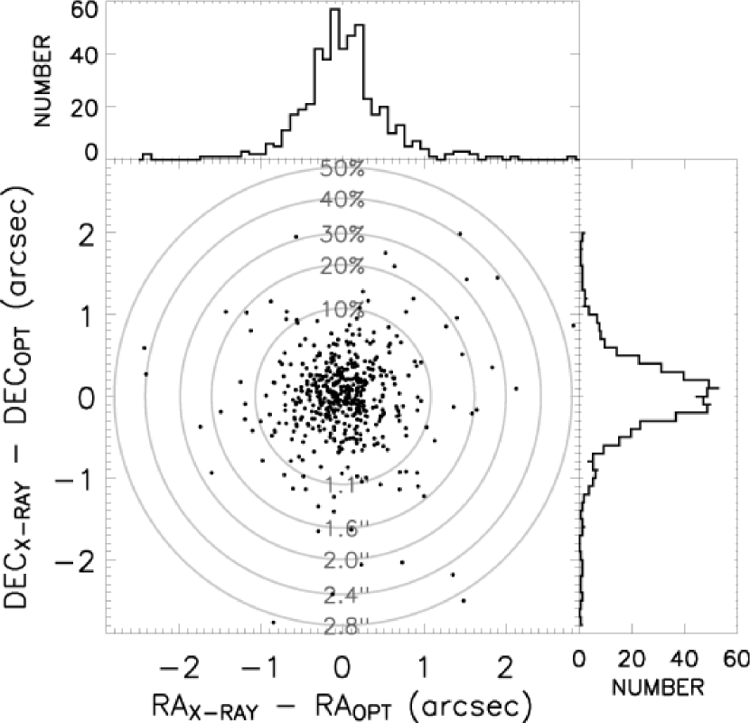
Figure 1: (X-ray $-$ optical) astrometric offsets for the 484 CLASXS sources with detected optical counterparts. Histograms for the R.A. (decl.) separations are shown on top (right). The mean values for the R.A. and decl. offsets are both $0.0\pm 0.5$ arcseconds. Concentric grey circles represent the probability of a source with a random R.A. and decl. being assigned an optical counterpart. The probabilities and search radii (in arcseconds) are given, respectively, at the top and bottom of each circle.

In Figure 1, we show the (X-ray $-$ optical) astrometric offsets for the CLASXS sources. Histograms for the right ascension and declination offsets are shown above and to the right, respectively. The average astrometric discrepancies in both axes are $0.0\pm 0.5$ arcseconds. We ran simulations to examine the probability of an X-ray source being assigned an incorrect optical counterpart. The probability of a chance projection is a strong function of the limiting optical magnitude in the catalog, since there are many more sources at the faint end. The concentric circles represent the probability of a source with a random right ascension and declination being assigned an optical counterpart from the full optical catalog ($R<27.9$). The inner circle is 10%, and the other circles increase outward with 10% increments. The majority of CLASXS sources have (X-ray $-$ optical) separations of less than $0.5\arcsec$ ($1~{}\sigma$) for which there is only a 2% probability of an incorrect X-ray/optical match. With our search radius of $2\arcsec$, we calculate that 30% of the CLASXS sources that in fact have no optical counterpart will be assigned an incorrect optical counterpart. Almost all of these will be with optically faint sources. If we limit the optical sources to those spectroscopically accessible ($R<24$), we find only an 8% chance of an incorrect X-ray/optical overlap using a $2\arcsec$ matching radius.

We show $R$-band thumbnails for 521 of the 525 CLASXS X-ray sources in the Y04 catalog in Figure 12 in the Appendix, ordered by increasing right ascension. Four X-ray sources (192, 318, 328, and 359) are outside the fields of view of our optical images and are not included. Stars are labeled “star”. Optically undetected sources are labeled “B” for “blank”. Spectroscopically observed sources that could not be identified are labeled “obs”.

4 Spectroscopic Observations

Optical spectra were obtained using the multi-fiber spectrograph HYDRA (Barden et al. 1994) on the WIYN 3.5 m telescope for bright ($I<19$) sources, and with the Deep Extragalactic Imaging Multi-Object Spectrograph (DEIMOS; Faber et al. 2003) on the 10 m Keck II telescope for fainter sources. Table 4 summarizes the telescopes, instruments, and dates of the spectroscopic observations.

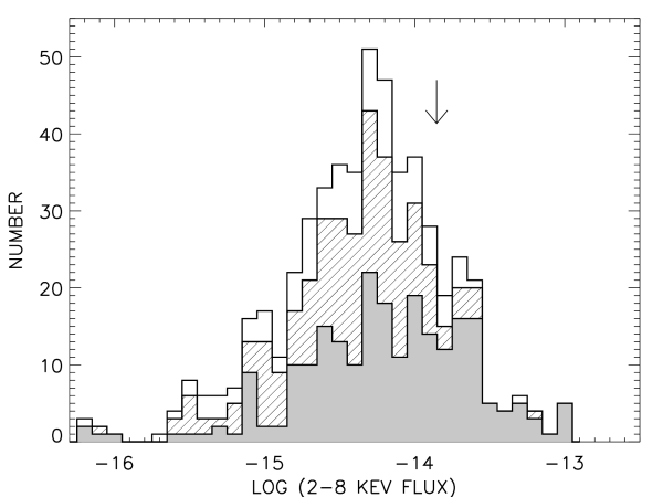
Figure 2: $2-8$ keV flux distribution for the 525 CLASXS sources (shaded, spectroscopic redshifts; hatched, spectroscopically observed sources that could not be identified; open, spectroscopically unobserved sources). The arrow marks the flux where the source contribution to the $2-8$ keV XRB peaks.

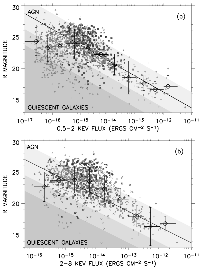
Figure 3: (a) The $R$ magnitude vs. $0.5-2.0$ keV flux for the soft X-ray sources in CLASXS (squares; Y04), the CDF-N (upward-pointing triangles; Barger et al. 2003), the CDF-S (downward-pointing triangles; Szokoly et al. 2004), and in combined ROSAT (Lehmann et al. 2001), XMM-Newton (Mainieri et al. 2002), and ASCA (Akiyama et al. 2003) surveys (plus signs). (b) The $R$ magnitude vs. $2-8$ keV flux for the hard X-ray sources (symbols as in (a); Lehmann et al. ROSAT sources have no hard X-ray measurements). In (b) we added the hard X-ray data from the HELLAS2XMM survey (crosses; Fiore et al. 2003). In both (a) and (b), the solid line shows where the fluxes are equal (i.e., log$(f_{X}/f_{R})=0$). The lightly shaded region covers log$(f_{X}/f_{R})=\pm 1$, where AGNs typically reside. Quiescent galaxies are usually found in the darkest shaded region (log$(f_{X}/f_{R})<-2$). Median magnitudes and fluxes for the X-ray sources from Tables 5 and 6 are shown as large diamonds with $1\sigma$ ranges shown as error bars. [A color version of this figure is available in the electronic edition of the Astronomical Journal.]

For the HYDRA observations, we used a low-resolution grating, 316@7.2, centered at 7600 Å, yielding a wavelength coverage of $4900-10300$ Å with a resolution of 2.64 Åpixel^-1. The red bench camera was used with the 2″ “red” HYDRA fibers to maximize the sensitivity at longer wavelengths. To obtain a wavelength solution for each fiber, CuAr comparison lamps were observed in each HYDRA configuration. Our HYDRA masks were designed to maximize the number of optically bright sources in each configuration, while minimizing the amount of overlap between configurations. Fibers that were unable to be placed on a source were assigned to a random sky location. We observed 2.7 hrs on two HYDRA configurations in 2001 February, 7.4 hrs on two configurations in 2002 February , and 6.0 hrs on two configurations in 2002 March. To remove fiber-to-fiber variations, on-source observations were alternated with $\pm 7.5\arcsec$ “sky” exposures taken with the same exposure times. This effectively reduced our on-source integration times to 1.3, 3.6, and 3.0 hrs in 2001 February, 2002 February, and 2002 March, respectively.

Reductions were performed using the standard IRAF package DOHYDRA. To optimize sky subtraction, we performed a two-step process. In the first step, the DOHYDRA routine was used to create an average sky spectrum using the fibers assigned to random sky locations. This average sky spectrum was then removed from all of the remaining fibers. In the offset images, this step effectively removed all of the sky signal, leaving behind only residuals caused by differences among the fibers. To remove these variations, we then subtracted the residuals present in the sky-subtracted offsets from the sky-subtracted, on-source spectra. We found this method to be very effective at removing the residuals created by fiber-to-fiber variations with HYDRA.

For the DEIMOS observations, we used the 600 lines mm^-1 grating, which yielded a resolution of 3.5 Å and a wavelength coverage of 5300 Å. The exact central wavelength depends upon the slit position, but the average was 7200 Å. Each $\sim 1$ hr exposure was broken into 3 subsets. In each subset the object was stepped 1.5″ in each direction. The DEIMOS spectroscopic reductions follow the same procedures used by Cowie et al. (1996) for LRIS reductions. The sky contribution was removed by subtracting the median of the dithered images. Cosmic rays were removed by registering the images and using a cosmic ray rejection filter on the combined images. Geometric distortions were also removed and a profile-weighted extraction was applied to obtain the spectrum. Wavelength calibration was done using a polynomial fit to known sky lines rather than using calibration lamps. The spectra were individually inspected and a redshift was measured only for sources where a robust identification was possible. The high-resolution DEIMOS spectra can resolve the doublet structure of the [O II] $\sim 3727$ Å line, allowing spectra to be identified by this doublet alone.

Figure 2 shows the $2-8$ keV flux distribution for the CLASXS sources. The sources that were spectroscopically observed (hatched) and spectroscopically identified (solid) are indicated. The arrow marks the flux where the source contribution to the $2-8$ keV XRB peaks. Of the 525 CLASXS sources detected in Y04, we have spectroscopically observed 467 (90%) and identified 271 (52%), including 20 stars.

5 Optical Properties of the X-ray Sources

Tables 5 and 6 give the median optical magnitudes for the CLASXS soft and hard X-ray sources, respectively. The tables also give, in parentheses, the median optical magnitudes for the CLASXS sources combined with other observations from Chandra (Barger et al. 2003; Szokoly et al. 2004), ROSAT (Lehmann et al. 2001), XMM-Newton (Mainieri et al. 2002; Fiore et al. 2003), and ASCA (Akiyama et al. 2003). Figure 3 shows the R magnitudes of the combined samples versus (a) soft and (b) hard X-ray flux. Any of the published X-ray catalogs that used energy ranges for the soft and hard bands other than $0.5-2$ keV and $2-8$ keV, respectively, were converted to this range using the power law assumed by the respective authors, or, if none were given, then by assuming a power law of $\Gamma=1.8$ and no absorption. The CLASXS sources with optical upper limits are denoted by arrows. CLASXS sources brighter than $R=20$ are typically saturated in our images, so the measured magnitudes of these sources may be underestimated.

The shaded regions in Figures 3a and 3b represent typical ranges of log$(f_{X}/f_{R})$ for different source classes (e.g., Alexander et al. 2002; Bauer et al. 2002; Barger et al. 2003). The flux in the R-band, $f_{R}$, is related to the R magnitude by log$(f_{R})=-5.5-0.4R$ (Hornschemeier et al. 2001). AGNs typically lie in or above the region defined by the loci log$(f_{X}/f_{R})=\pm 1$ (lightest shading), while normal galaxies lie below log$(f_{X}/f_{R})<-2$ (darkest shading). Note that the flux limit of the CLASXS survey ($f_{2-8{\rm keV}}>3\times 10^{-15}$ ergs cm^-2 s^-1) makes it an AGN dominated survey.

The median $R$-band magnitudes in each flux bin (see values in parentheses in Tables 4 and 5) are shown in Figure 3 as the large diamonds with $1\sigma$ standard deviations for each flux bin, denoted by error bars. The median X-ray/optical flux ratios for the soft X-ray sources follow the log$(f_{X}/f_{R})=0$ loci for fluxes larger than $f_{0.5-2~{}{\rm keV}}\geq 5\times 10^{-16}$ ergs cm^-2 s^-1, but drop to smaller X-ray/optical ratios at fainter X-ray fluxes. As noted by Barger et al. 2003, the explanation for this is straightforward. At bright soft X-ray fluxes, the AGNs usually dominate the X-ray and optical light, so the galaxies follow a constant X-ray/optical flux ratio. At fainter X-ray fluxes, the starlight begins to dominate over the optical AGN contributions, possibly as a result of obscuration, an increase in the number of intrinsically lower luminosity AGNs, or, at the faintest fluxes, an increase in the number of galaxies without AGNs (e.g. Hornschemeier et al. 2003). Since stars contribute less than the AGNs to the X-ray emission, the result is a drop in the X-ray/optical flux ratios. In addition, any intrinsic obscuration will also attenuate the soft X-ray emission from the central engine. For near Compton-thick AGNs, all of the soft X-ray and optical AGN light will be attenuated.

The $R$-magnitudes shown in Figure 3 are not nuclear magnitudes, so they differ from the optical/X-ray studies done of nearby Seyfert galaxies. We use a fixed aperture for our photometric measurements that covers a varying fraction of the optical counterpart. This fraction is dependent on the apparent angular size of the optical source and can vary between the nuclear magnitude for nearby sources and the total magnitude for high-redshift sources. This introduces a scatter in the y-axis of Figure 3, because a high-redshift source will have a brighter optical magnitude than its low-redshift twin. Since most of our sources have small angular sizes (see Figure 12), our $R$-band magnitudes can be considered upper limits to the nuclear $R$-band magnitudes. In other words, if we could measure only the nuclear magnitudes for the CLASXS sources, then the observed $R$-band magnitudes would decrease. This would shift many CLASXS sources away from the Quiescent Galaxies regime and into the AGN regime.

5.1 AGN Obscuration

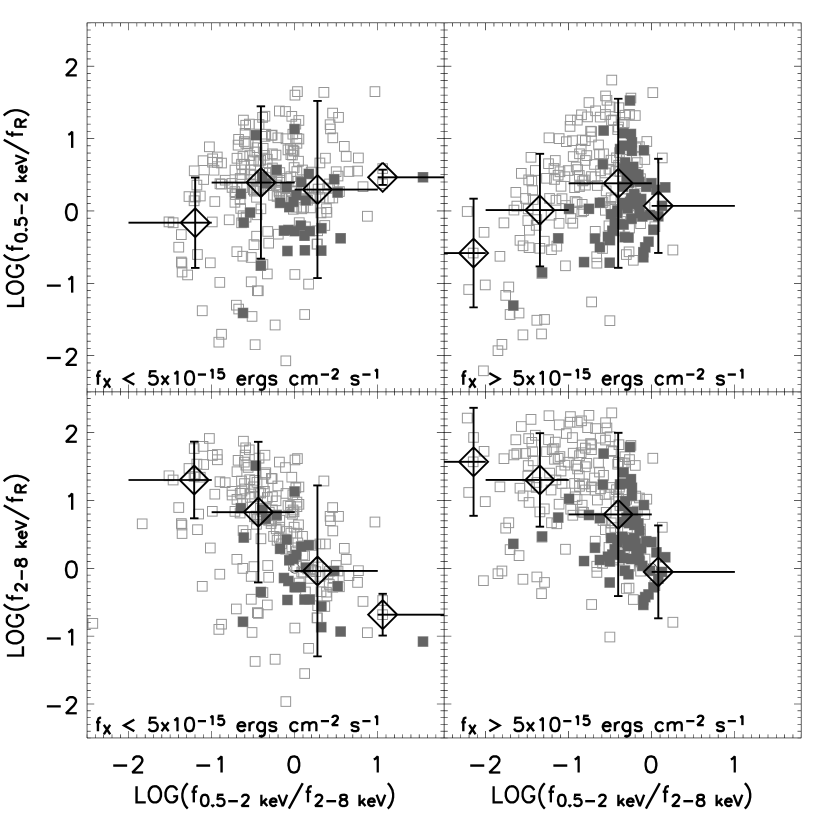
Figure 4: Soft and hard X-ray–to–optical flux ratios for the CLASXS soft and hard X-ray–selected sources vs. soft to hard X-ray flux ratio. The samples were further broken into two populations: X-ray bright ($f_{2-8~{}{\rm keV}}>10^{-15}$ ergs cm^-2 s^-1) and X-ray faint ($f_{2-8~{}{\rm keV}}<10^{-15}$ ergs cm^-2 s^-1). Sources identified as stars are not shown. BLAGNs are shown as solid squares and non-BLAGNs as open squares. The average flux ratio is shown as large open diamonds for each logarithmic soft-to-hard flux ratio bin.

The presence of an obscuring torus can affect the X-ray/optical flux ratio of a source, depending on which X-ray band we examine. Since a photon’s cross-section decreases rapidly with increasing photon energy, light from the near-infrared to soft X-rays is typically attenuated in moderately obscured AGNs, while hard X-ray light penetrates all but the most obscured sources.

Figure 4 shows the $0.5-2$ keV to $R$-band and $2-8$ keV to $R$-band flux ratios versus soft-to-hard X-ray flux ratio for the CLASXS soft and hard X-ray selected samples. The samples were further separated by hard X-ray flux into bright ($f_{2-8~{}{\rm keV}}>10^{-15}$ ergs cm^-2 s^-1) and faint ($f_{2-8~{}{\rm keV}}<10^{-15}$ ergs cm^-2 s^-1) categories. The filled squares denote broad-line AGNs (BLAGNs). The large diamonds are the average $\log(f_{X}/f_{R})$ within the soft-to-hard flux ratio ranges of $\log(f_{0.5-2~{}{\rm keV}}/f_{2-8~{}{\rm keV}})=(-2,-1)$, $(-1,0)$, $(0,1)$, $(1,2)$, and $(2,3)$.

We expect that for the $0.5-2$ keV X-ray/optical flux ratio, the presence of any obscuring material will attenuate both the soft X-ray and optical photons, making the flux ratio only weakly dependent on the column density for unobscured to moderately obscured sources. Moreover, for highly obscured sources, the AGN contribution to both the observed soft X-ray and optical light should become negligible, causing the galaxy to descend into the “Quiescent Galaxy” category.

If we treat the soft-to-hard flux ratio as an approximation to the line-of-sight column density (column density would decrease with increasing soft-to-hard X-ray flux ratio), we can see from Figure 4 that the soft X-ray/optical flux ratio (top row) does indeed remain relatively constant for $\log(f_{0.5-2~{}{\rm keV}}/f_{2-8~{}{\rm keV}})>-1$. Moreover, at larger column densities, where both the optical and the soft X-ray light are obscured, there may be a slight drop in the soft X-ray/optical flux ratio as the AGN contributions to both become negligible and the optical starlight from the galaxy begins to dominate.

In contrast, we expect that moderate column densities of material will not significantly attenuate the hard X-ray photons from an AGN, so moderately obscured sources will have high hard X-ray/optical flux ratios. From Figure 3 (bottom row), we see that as the column density increases, the AGN’s optical light is blocked, while the hard X-rays can still penetrate the material. Thus, the hard X-ray/optical flux ratio increases until the material becomes opaque to hard X-rays. At these high column densities, even the X-ray light is absorbed, and we would expect to see the X-ray/optical flux ratio begin to drop. However, near-Compton-thick sources are very X-ray weak and difficult to detect, and there may be very few of them in the sample.

The aforementioned trends in the soft and hard X-ray-to-optical ratios appear to hold for both the X-ray bright and faint CLASXS sources. However, there are noticeable differences in the two populations that can be seen in Figure 4. There is a significantly larger population of BLAGNs in the X-ray bright population than in the X-ray faint population. This is consistent with the discovery by Steffen et al. (2003) that the BLAGNs dominate the number densities at the higher X-ray luminosities, while the non-BLAGNs dominate at the lower X-ray luminosities.

6 Spectroscopic Properties

The redshift distribution of the CLASXS sources is shown in Figure 5. The two histograms have $\Delta z=0.1$ and $\Delta z=0.01$ width bins. There are no obvious structures at $z<1$ in the CLASXS redshift distribution, unlike the apparent excesses found at $z=0.48$ and $z=0.94$ in the CDF-N sample by Barger et al. (2003), and at $z=0.674$ and $z=0.734$ in the CDF-S sample by Gilli et al. (2003) and Szokoly et al. (2004). (There might be a grouping of CLASXS sources at $z=1.8$, though this is not easily seen in the figure.) The differences between the redshift distributions of CLASXS and the CDFs show that we have indeed sampled a large enough area in CLASXS to average out the large scale structure.

Figure 5: Redshift distribution for the spectroscopically identified CLASXS sources. All stars and sources without measured redshifts have been excluded. Two different bin sizes ($\Delta z=0.1$ and $\Delta z=0.01$) are shown.

Following Cowie et al. (2004a), we optically classified sources into four categories, roughly using the procedure of Sadler et al. (2002) to analyze low-redshift radio samples. We classified sources without any strong emission lines (EW([O II])$<3$Å or EW(H$\alpha+$N II $<10$Å) as absorbers; sources with strong Balmer lines and no broad or high-ionization lines as star formers; sources with [Ne V] or C IV lines or strong [O III] (EW([O III] 5007 Å) $>3$ EW(H$\beta$)) as Seyfert galaxies; and, finally, sources with lines with FWHM $>1000$ km s^-1 as BLAGNs. Table 7 breaks down the identified sources by spectral type.

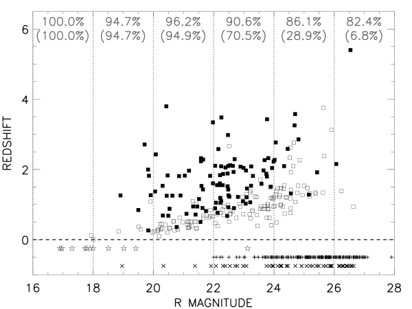
Figure 6: Redshift vs. R-band magnitude for the CLASXS hard X-ray sample (stars, stars placed at $z=-0.25$; plus signs,spectroscopically observed but unidentified sources placed at $z=-0.5$; crosses,spectroscopically unobserved sources placed at $z=-0.75$; filled squares,BLAGNs; open squares—non-BLAGNs). The graction of the CLASXS sources that have been spectroscopically observed (identified) for each bin of $\Delta R=2$ mag (dotted lines) is shown across the top of the figure.

Figure 6 shows redshift versus $R$-band magnitude for the CLASXS hard X-ray sample, with BLAGNs denoted by solid squares and non-BLAGNs denoted by open squares. Figure 7 combines the CLASXS data with the data of Barger et al. (2003), Mainieri et al. (2002), and Szokoly et al. (2004), dividing the X-ray sources into BLAGNs and non-BLAGNs. To remove the bias introduced by the depth of the CDF-N survey, which is deep enough to detect the X-ray emission from nearby galaxies with no AGN component, we have only shown the sources with $f_{2-8~{}{\rm keV}}>3\times 10^{-15}$ ergs cm^-2 s^-1. The combined surveys have very few BLAGNs at $z<0.5$, but the numbers increase at $z=0.5$ and appear to decrease only slightly over the range $z\sim 0.5-2.5$ before falling off beyond. The redshift distribution is quite different for the non-BLAGN population. However, there are strong selection effects in the spectroscopic identifications. There are many more AGNs at low redshifts that do not have broad optical emission lines, either because of low intrinsic AGN luminosity or obscuration. Thus, the identifications for these sources are based on their galaxy spectra, and at high redshifts, galaxy spectra are much harder to spectroscopically identify than BLAGN spectra, particularly in the spectroscopic redshift desert at $z=1.5-2$ (e.g., Wirth et al. 2004; Cowie et al. 2004b).

Figure 7: Redshift distribution of (a) BLAGNs and (b) non-BLAGNs with $f_{2-8~{}{\rm keV}}>3\times 10^{-15}\ \mbox{ergs cm${}^{-2}$ s${}^{-1}$}$ (see § 6) in four surveys: CLASXS, CDF-N (Barger et al. 2003), CDF-S (Szokoly et al. 2004), and XMM-Newton Lockman Hole (Mainieri et al. 2002). All stars and sources without measured redshifts have been excluded.

7 Colors and Luminosities of the CLASXS sources

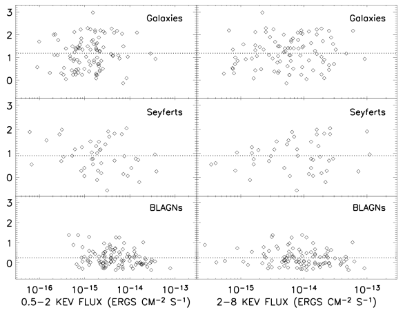
Figure 8: B$-$R color vs. soft (left) and hard (right) X-ray flux for three spectral classes (normal galaxies, Seyferts, and BLAGNs) for the CLASXS sources. The dotted lines denote the median $B-R$ colors for each spectral class.

In Figures 8a and 8b, we plot the observed B$-$R color versus soft and hard flux for the spectroscopically identified CLASXS sources with $R<26$, excluding any sources that are saturated. We break the sources into three spectroscopic categories: BLAGNs, Seyfert galaxies, and “normal” galaxies (the last category combines the absorbers and star formers classes of § 6). The BLAGNs are, on average, much bluer than the other types of sources. This is due to the excess blue continuum from the AGN itself that is commonly observed in unobscured (type I) AGNs. Thus, the colors and the spectroscopic classes are in good agreement.

Figure 9: Distribution of absolute rest-frame $B$ magnitude for all of the CLASXS sources with measured redshifts less than $z=1.07$ (open histogram). BLAGNs (non-BLAGNs) are shown as a solid (hatched) histogram. (See § 7 for an explanation of the redshift limit.)

The distribution of the absolute rest-frame B magnitudes for the CLASXS sources is shown in Figure 9, calculated using the measured redshift and interpolating the B-magnitude in the observer’s rest-frame from the observed broadband colors. Since we do not have near-infrared observations of all of our X-ray sources, we can only use this technique to measure absolute B-magnitudes for sources with $z<1.07$. Beyond this redshift, the rest-frame B-band moves redward beyond our $z^{\prime}$ observations. Only non-stellar sources with measured magnitudes in at least two wavebands are included. BLAGNs and non-BLAGNs are shown as solid and hatched histograms, respectively.

Our photometric data do not have the resolution necessary to separate the luminosity of the host galaxy from that of the central AGN, so we can only comment on the combined AGN+host luminosity. Since BLAGNs have an excess blue continuum, one would expect a larger number of BLAGNs at brighter absolute B magnitudes. Indeed, Figure 9 shows that this is the case.

8 Discussion

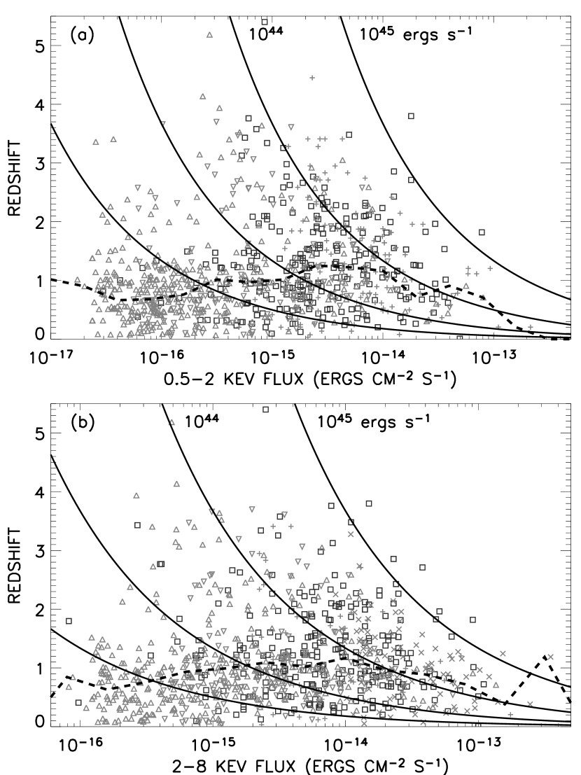
Figure 10: (a) Redshift vs. $0.5-2.0$ keV flux for the soft X-ray–selected sources in CLASXS (squares), the CDF-N (upward-pointing triangles; Barger et al. 2003), the CDF-S (downward-pointing triangles; Szokoly et al. 2004), and in combined ROSAT (Lehmann et al. 2001), XMM-Newton (Mainieri et al. 2002), and ASCA (Akiyama et al. 2003) surveys (plus signs). (b) Redshift vs. $2-8$ keV flux for the hard X-ray selected sources (symbols as in (a); Lehmann et al. ROSAT sources have no hard X-ray measurements). In (b) we added the hard X-ray data from the HELLAS2XMM survey (crosses; Fiore et al. 2003). Dashed lines show the median redshift of the combined samples versus soft and hard X-ray flux. [A color version of this figure is available in the electronic edition of the Astronomical Journal.]

Figure 11: Rest-frame hard X-ray luminosity of the CLASXS (squares), CDF-N (upward-pointing triangles; Barger et al. 2003), HELLAS2XMM (crosses; Fiore et al. 2003), XMM-Newton Lockman Hole (diamonds; Mainieri et al. 2002), and CDF-S (downward-pointing triangles; Szokoly et al. 2004) sources with known redshifts. CDF-N sources with spectroscopic (photometric) redshifts are shown as open (filled) symbols. Curves represent the on-axis flux limits for the different surveys (see legend). Right-hand axis shows the accretion rate (in solar masses per year). [A color version of this figure is available in the electronic edition of the Astronomical Journal.]

In Figures 10a and 10b, we plot redshift versus soft and hard X-ray flux for the combined samples of § 5. The data and symbols are identical to those in Figure 3. The CLASXS data nicely fill in the intermediate flux interval between the deep Chandra data and the shallower ASCA and ROSAT data. The dashed lines show the median redshifts of the combined samples versus soft and hard X-ray flux. The median redshifts remain around $z\sim 1$ and do not appear to be strongly correlated with either soft or hard X-ray flux. Of course, the redshift determinations depend on the optical magnitudes of the sources. Since the magnitudes of high-redshift sources may be faint, these surveys might be biased against finding high-redshift sources. The solid lines denote constant rest-frame X-ray luminosities, which were calculated assuming a $\Gamma=1.8$ power-law spectral energy distribution with no absorption. They range from $10^{42}$ to $10^{45}$ ergs s^-1; the two largest luminosities are labeled. Any source more luminous than $L_{X}=10^{42}$ ergs s^-1 is very likely to be an AGN on energetic grounds (Zezas, Georgantopoulos, & Ward 1998; Moran, Lehnert, & Helfand 1999), though many of the intermediate luminosity sources do not show obvious AGN signatures in their optical spectra (e.g., Barger et al. 2001b; Hornschemeier et al. 2001; Tozzi et al. 2001).

We use the hard X-ray fluxes and redshifts of the combined samples in Figure 10b to calculate the rest-frame hard X-ray luminosities. As in § 2, we assume a power law spectral energy distribution with $\Gamma=1.8$ for calculating the K-corrections to determine the rest-frame hard X-ray luminosities. Using a universal power law index rather than individual indices to calculate the K-corrections results in only a small difference in the calculated luminosities (Barger et al. 2002). Figure 11 shows the rest-frame hard X-ray luminosities for the hard X-ray sources and limiting fluxes of the CLASXS, Barger et al. (2003), Fiore et al. (2003), Mainieri et al. (2002), and Szokoly et al. (2004) catalogs. The CLASXS X-ray sample has the largest number of $L_{2-8~{}{\rm keV}}\geq 10^{45}~{}{\rm ergs~{}s}^{-1}$ sources. Even with the increased solid angle covered by the five surveys, there is an obvious lack of extremely luminous ($L_{2-8~{}{\rm keV}}\geq 10^{44}~{}{\rm ergs~{}s}^{-1}$) AGNs at $z<0.5$.

The bolometric luminosity, $L_{BOL}$, of an AGN is related to the rate of accretion, $\dot{M}$, onto its supermassive black hole using the expression $\epsilon\dot{M}_{BH}=L_{BOL}/c^{2}$, where $c$ is the speed of light and $\epsilon$ is the accretion efficiency (typically, $\epsilon\sim 0.1$). Because AGNs are luminous from radio to X-ray energies, multiwavelength observations are needed to accurately calculate their bolometric luminosities. If we use a bolometric correction of 35 (Elvis et al. 1994; Barger et al. 2001b; Kuraszkiewicz et al. 2003) appropriate for the type I AGNs to translate hard X-ray luminosity, $L_{X}$, to $L_{BOL}$ and assume an efficiency of $\epsilon=0.1$, then we can roughly estimate the accretion rates. The results are shown in Figure 11 (right-hand axis). The small solid angle of the CDF-N survey prevented Barger et al. (2001a) from determining if the lack of low redshift, high luminosity sources in their sample were due to an actual deficiency of these sources at low redshifts or simply a selection effect owing to the small local volume sampled and the low spatial density of these sources. CLASXS samples a larger local cosmological volume to better constrain the accretion rate at low redshifts, and we can now clearly see that the deficiency of these sources is indeed real and that at $z<0.5$ there are very few sources with accretion rates above a solar mass per year.

9 Summary

We have presented optical photometric and spectroscopic observations of the X-ray sources in the CLASXS survey. We obtained $BVRIz^{\prime}$ photometry for 521 of the 525 X-ray sources in the sample. We spectroscopically observed 467 of the CLASXS sources, obtaining redshift identifications for 271. The positions of the sources in our optical catalog agree well with the X-ray catalog, with average astrometric offsets of $0.0\pm 0.5$ arcseconds in both right ascension and declination.

Using our optical data, we have examined the relationship between the X-ray and optical source properties. We find that the average soft X-ray–to–optical flux ratio remains relatively constant for CLASXS sources with low to moderate column densities of obscuring material. Conversely, the hard X-ray–to–optical flux ratio for these sources appears to be correlated with line-of-sight column density. Because of the large solid angle covered by CLASXS, we do not find the low-redshift structures that are seen in narrower, deeper Chandra surveys. However, we do detect a possible excess of sources at $z=1.8$. Using hard X-ray catalogs from five Chandra and XMM-Newton surveys we find that there is a distinct lack of luminous, high-accretion rate sources at low redshifts ($z<1)$, consistent with previous observations which showed that supermassive black hole growth is dominated at low redshifts by sources with low accretion rates (Barger et al. 2001a).

Appendix A Appendix

Details of the Lockman Hole-Northwest photometric observations and reductions can be found in Capak et al. (2004b). We provide a short summary of the Subaru and CFHT broadband photometric observations here. For the Subaru images, bad pixels and chip gaps were filled in by creating mosaics using a five point star-shaped dither pattern with $1\arcmin$ steps. The separation between dithered images was made large enough to create deep sky flats during the image reduction process. The camera was rotated by $90\deg$ between dithers to remove bleeding from bright stars and provide better photometric calibration. The Suprime-Cam data cover the central $36^{\prime}\times 36^{\prime}$ of the field, but only the central $27^{\prime}\times 27^{\prime}$ of the Suprime-Cam field goes to the full depth due to vignetting in Suprime-Cam. In the R band, we added four Suprime-Cam pointings covering $54^{\prime}\times 54^{\prime}$ from the Subaru archive. These data were collected using the same dither pattern and reduced by us in the same manner as our other data. For the CFHT observations, a standard seven point circular dither pattern was used. The radius of the dither circle was $7.5^{\prime\prime}$, which was enough to fill the chip gaps but minimized the chip overlap. The observing time was divided between two pointings separated by $14^{\prime}$ in the north-south direction. This allowed us to cover a $42^{\prime}\times 42^{\prime}$ field while going deeper in a central strip.

All the data were reduced using Nick Kaiser’s IMCAT tools. Flat-fielding of the CFHT images was done using ELIXIR. The $z^{\prime}$ data were corrected for fringing. The images were aligned astrometrically using a self-consistent astrometric solution described in Capak et al. (2004a). The solution was calculated using the CFHT $R$-band data along with wide-field Suprime-Cam data. The USNO-B1.0 (Monet et al. 2003) was used as the reference catalog for this process and provided the absolute astrometric zeropoint. All other data were warped onto this $R$-band image. The individual mosaics were then combined. Thumbnails of 521 sources are shown in Figure 12.

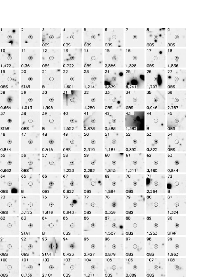
Figure 12: $R$-band thumbnails of 521 of the 525 CLASXS. Four X-ray sources (192, 318, 328, and 359) are outside the fields-of-view of our optical images. The $R$-band $2\sigma$ AB magnitude limit is 27.9. Thumbnails are 15″ on a side. Y04 source number (column [1] of Table 1 in this paper) is displayed in the top left corner. If an X-ray source has an optical counterpart, then a 3″ aperture is shown centered on the optical counterpart. If there is no detected counterpart, then the 3″ aperture is centered on the X-ray position. Redshifts for identified optical counterparts are shown in the bottom left corner. Stars are labeled “star”. Optically undetected sources are labeled “B” for blank. Spectroscopically observed sources that could not be identified are labeled “obs”.

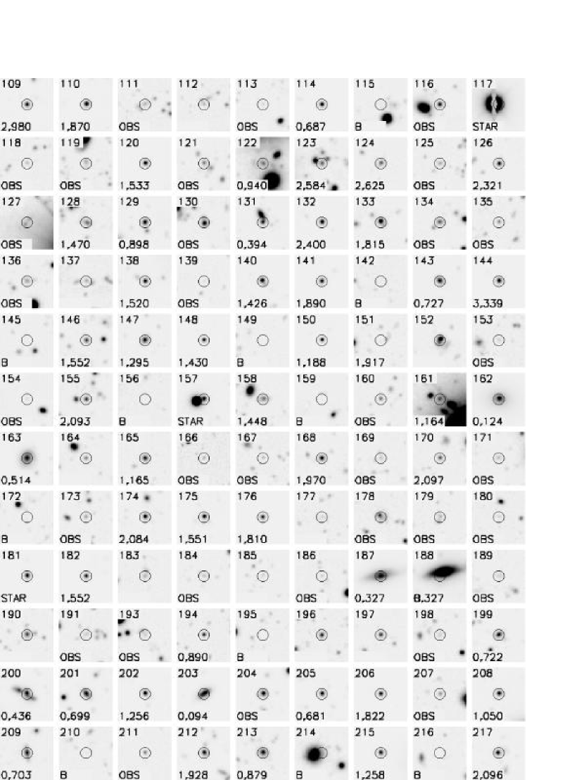
Figure 12: cont’d

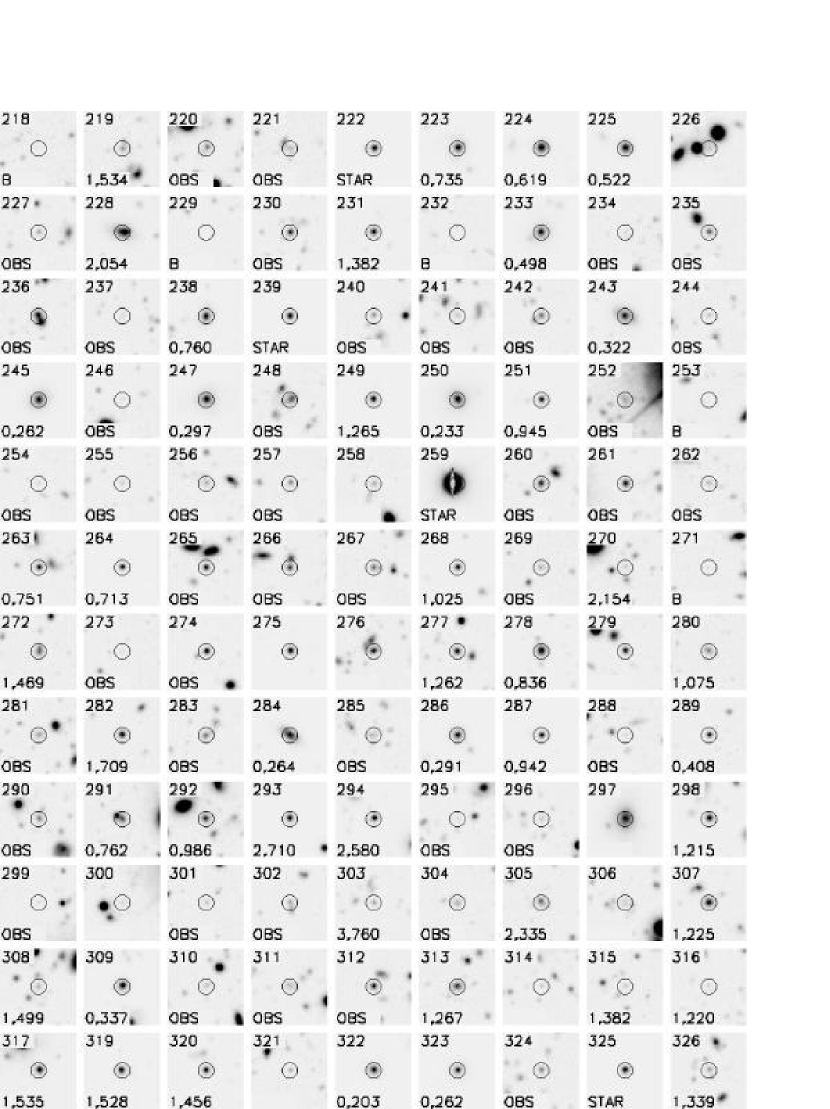
Figure 12: cont’d

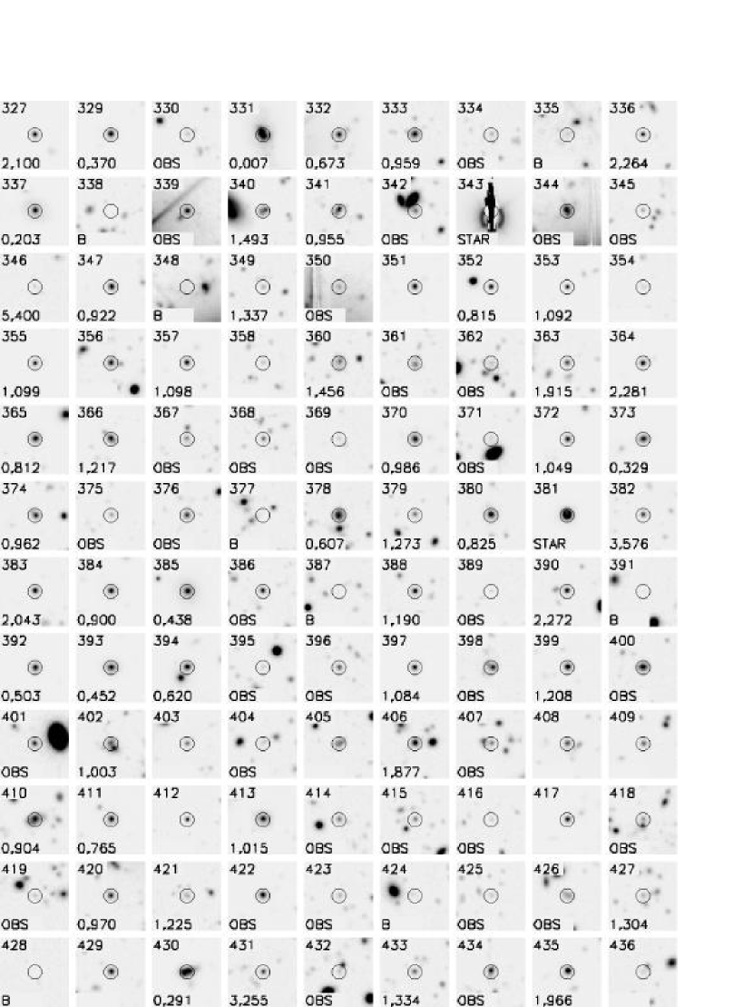
Figure 12: cont’d

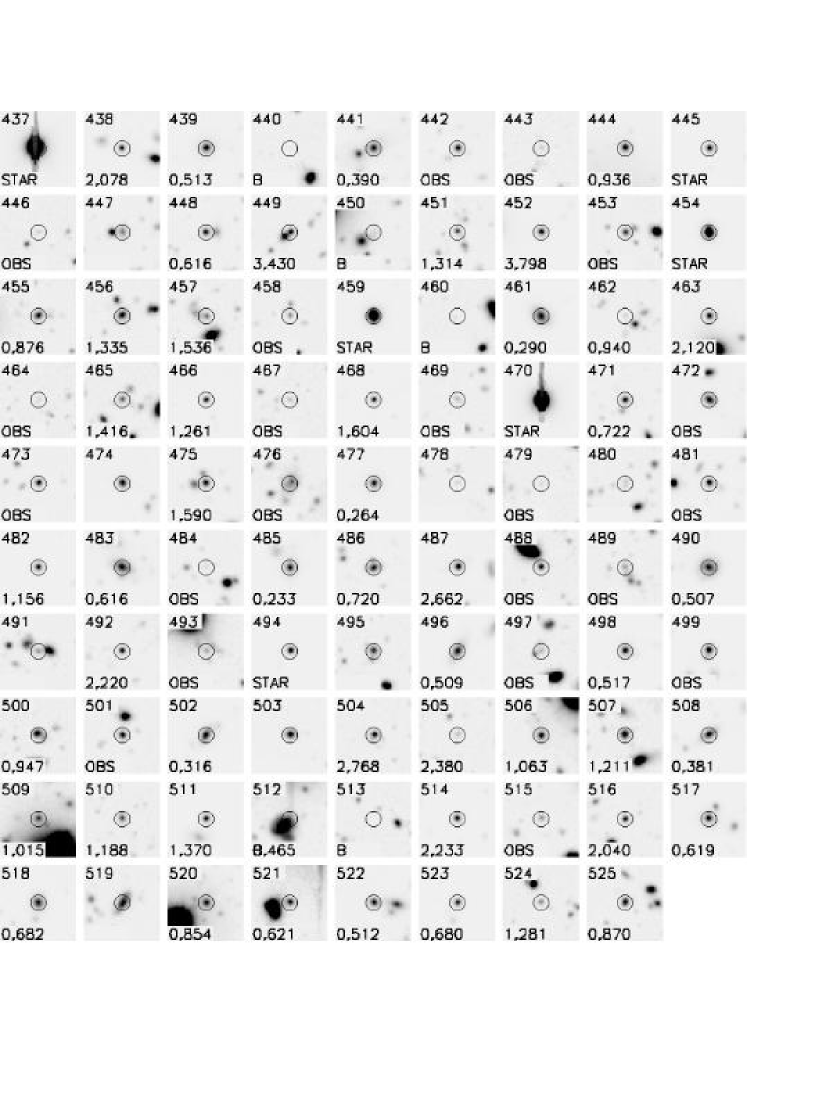
Figure 12: cont’d

In Table 1 we present optical magnitudes and spectroscopic measurements, where available, for the CLASXS X-ray point source catalog of Y04. The 525 X-ray sources are ordered by increasing right ascension and are labeled with the Y04 source number (col. [1]). The right ascension and declination coordinates of the X-ray sources are given in columns (2) and (3), and the smallest off-axis angle is given in column (4). The right ascension and declination coordinates of the optical counterparts are given in decimal degrees in columns (5) and (6). The soft ($0.5-2$ keV) and hard ($2-8$ keV) X-ray fluxes, abbreviated SB and HB, are given in columns (7) and (8). The aperture corrected, broadband B, V, R, I, and $z^{\prime}$ apparent magnitudes are given in columns (9)-(13). The aperture correction was calculated by examining the curve-of-growth for isolated, moderately bright ($R=20-26$) sources. The 3″ aperture corrections for the Subaru (CFHT) images are $-0.17$ ($-0.30$), $-0.22$, $-0.11$ ($-0.15$), $-0.33$, $-0.13$ ($-0.22$), for the B, V, R, I, and $z^{\prime}$ bands, respectively. Sources that fall outside of the field-of-view of a given filter are left blank. If a source falls within the field-of-view, but is not detected, then it is assigned the $2\sigma$ magnitude limit for that filter and is considered an upper limit. The spectroscopic redshifts are given in column (14).

Table 1: Optical Properties of the CLASXS X-ray Sample

	X-ray (J2000.0)			Optical (J2000.0)
Y04	R.A.	Decl.	$R_{aim}$	R.A.	Decl.	SB	HB	B	V	R	I	$z^{\prime}$	$z_{spec}$
(1)	(2)	(3)	(4)	(5)	(6)	(7)	(8)	(9)	(10)	(11)	(12)	(13)	(14)
1	157.731750	57.55556	9.99	157.730803	57.55546	3.42	3.70	$\cdots$	$\cdots$	23.1	$\cdots$	$\cdots$	$\cdots$
2	157.748667	57.64561	8.76	157.747566	57.64558	1.62	5.30	$\cdots$	$\cdots$	22.7	$\cdots$	$\cdots$	$\cdots$
3	157.763833	57.61400	8.16	157.763506	57.61356	2.88	13.00	$\cdots$	$\cdots$	23.5	$\cdots$	$\cdots$	obs
4	157.775250	57.63011	7.80	157.774430	57.63017	3.33	0.74	$\cdots$	$\cdots$	23.8	$\cdots$	23.4	obs
5	157.799292	57.58936	7.27	157.799617	57.58951	2.88	0.91	24.7	$\cdots$	24.0	$\cdots$	23.0	obs

Note. — The complete version of this table is in the electronic edition of the Astronomical Journal. The printed edition contains only a sample.

Table 2: Summary of Optical Imaging Observations: Telescopes, Dates of Observations, and Integration Times

Band	Telescope	UT Dates	Integration
			(hr)
$B$	Subaru 8.2 m	2001 February 27-28	1.7
$B$	CFHT 3.6 m	2002 December 4-5, 27-29	5.8
$V$	Subaru 8.2 m	2002 April 22-23	6.4
$R$	Subaru 8.2 m	2001 February 27-28	5.2
$R$	Subaru 8.2 m	2001 March 19-20	2.0
$R$	CFHT 3.6 m	2003 January 2-3, 25-30	11.9
$I$	Subaru 8.2 m	2001 April 21-22	0.9
$z^{\prime}$	Subaru 8.2 m	2001 April 21, 23	1.3
$Z$	CFHT 3.6 m	2002 December 27	11.9
$Z$	CFHT 3.6 m	2003 January 25-31	11.9

Table 3: Summary of Optical Images: Filters, Telescopes, Data Quality, Depth, and Area Coverage

Band	Telescope	Average seeing	$2~{}\sigma$ limit	Total area	Deep area
		(arcsecond)	(AB mag)	(deg2)	(deg2)
$B$	Subaru 8.2 m	0.96	27.8	0.27	0.20
$B$	CFHT 3.6 m	0.97	27.6	0.49	0.49
$V$	Subaru 8.2 m	1.15	27.5	0.36	0.20
$R$	Subaru 8.2 m	0.96	27.9	0.27	0.20
$R$	Subaru 8.2 m	0.61	27.7	0.81	0.81
$R$	CFHT 3.6 m	0.89	27.9	0.49	0.49
$I$	Subaru 8.2 m	1.30	26.4	0.36	0.20
$z^{\prime}$	Subaru 8.2 m	1.01	26.2	0.36	0.20
$Z$	CFHT 3.6m	0.95	26.3	0.49	0.49

Table 4: Summary of Spectroscopic Observations: Telescopes, Instruments, and Dates of Observations

Telescope	Instrument	UT Dates
WIYN 3.5m	HYDRA	2001 February 19-20
WIYN 3.5m	HYDRA	2002 February 6-7
WIYN 3.5m	HYDRA	2002 March 9-10
Keck II	DEIMOS	2003 January 28-29
Keck II	DEIMOS	2003 March 26
Keck II	DEIMOS	2003 April 24-26
Keck II	DEIMOS	2003 May 26
Keck II	DEIMOS	2004 January 17-19
Keck II	DEIMOS	2004 April 13-15

Table 5: Median R-band Magnitudes of the 0.5-2 keV CLASXS (combined) Sample

$0.5-2$ keV Flux Range
($10^{-16}$ ergs cm-2 s-1)	Number	Median $0.5-2$ keV Flux	R
1-3	36 (248)	$2.2\times 10^{-16}$ ($1.9\times 10^{-16}$)	24.7 (23.3)
3-10	149 (325)	$6.6\times 10^{-16}$ ($6.1\times 10^{-16}$)	24.6 (23.9)
10-30	190 (349)	$1.9\times 10^{-15}$ ($1.9\times 10^{-15}$)	23.4 (23.2)
30-100	92 (188)	$5.6\times 10^{-15}$ ($5.6\times 10^{-15}$)	22.4 (22.2)
100-300	37 (80)	$1.8\times 10^{-14}$ ($1.7\times 10^{-14}$)	20.6 (20.7)
300-1000	6 (31)	$4.6\times 10^{-14}$ ($5.5\times 10^{-14}$)	20.6 (18.6)

Table 6: Median R-band Magnitudes of the $2-8$ keV CLASXS (Combined) Sample

$2-8$ keV Flux Range	Number	Median $2-8$ keV Flux	R
($10^{-16}$ ergs cm-2 s-1)
1-3	6 (125)	$2.5\times 10^{-16}$ ($2.1\times 10^{-16}$)	24.4 (22.7)
3-10	47 (258)	$6.3\times 10^{-16}$ ($6.1\times 10^{-16}$)	23.7 (23.7)
10-30	98 (356)	$2.0\times 10^{-15}$ ($1.9\times 10^{-15}$)	24.1 (23.8)
30-100	197 (369)	$5.9\times 10^{-15}$ ($5.8\times 10^{-15}$)	24.0 (23.5)
100-300	113 (236)	$1.7\times 10^{-14}$ ($1.7\times 10^{-14}$)	22.5 (22.3)
300-1000	18 (64)	$5.4\times 10^{-14}$ ($5.4\times 10^{-14}$)	21.2 (20.7)
1000-3000	3 (70)	$1.0\times 10^{-13}$ ($1.8\times 10^{-13}$)	20.7 (18.0)

Table 7: Number of X-ray Sources Per Spectral Type For Identified CLASXS Sources

Class	Number	$\%$ of CLASXS Sample
Stars	20	4
Star Formers	73	14
Broad-line AGNs	106	20
Seyferts	44	8
Absorbers	28	5

References

- Akiyama et al. (2003) Akiyama, M., Ueda, Y., Ohta, K., Takahashi, T., & Yamada, T. 2003, ApJS, 148, 275
- Alexander et al. (2002) Alexander, D. M., Aussel, H., Bauer, F. E., Brandt, W. N., Hornschemeier, A. E., Vignali, C., Garmire, G. P., & Schneider, D. P. 2002, ApJ, 568, L85
- Alexander et al. (2003) Alexander, D. M., et al. 2003, AJ, 126, 539
- Baldi et al. (2002) Baldi, A., Molendi, S., Comastri, A., Fiore, F., Matt, G., & Vignali, C. 2002, ApJ, 564, 190
- Barden et al. (1994) Barden, S. C., Armandroff, T., Muller, G., Rudeen, A. C., Lewis, J., & Groves, L. 1994, Proc. SPIE, 2198, 87
- Barger et al. (2001a) Barger, A. J., Cowie, L. L., Bautz, M. W., Brandt, W. N., Garmire, G. P., Hornschemeier, A. E., Ivison, R. J., & Owen, F. N. 2001a, AJ, 122, 2177
- Barger et al. (2002) Barger, A. J., Cowie, L. L., Brandt, W. N., Capak, P., Garmire, G. P., Hornschemeier, A. E., Steffen, A. T., & Wehner, E. H. 2002, AJ, 124, 1839
- Barger et al. (2001b) Barger, A. J., Cowie, L. L., Mushotzky, R. F., & Richards, E. A. 2001b, AJ, 121, 662
- Barger et al. (2003) Barger, A. J., et al. 2003, AJ, 126, 632
- Bauer et al. (2002) Bauer, F. E., Alexander, D. M., Brandt, W. N., Hornschemeier, A. E., Vignali, C., Garmire, G. P., & Schneider, D. P. 2002, AJ, 124, 2351
- Bertin & Arnouts (1996) Bertin, E., & Arnouts, S. 1996, A&AS, 117, 393
- Brandt et al. (2001) Brandt, W. N., et al. 2001, AJ, 122, 2810
- Campana et al. (2001) Campana, S., Moretti, A., Lazzati, D., & Tagliaferri, G. 2001, ApJ, 560, L19
- Capak et al. (2004a) Capak, P., Cowie, L. L., Barger, A. J., & Hu, E. 2004a, AJ, 127, 180
- Capak et al. (2004b) Capak, P., et al. 2004b, in preparation
- Cowie et al. (2004a) Cowie, L. L., Barger, A. J., Fomalont, E. B., & Capak, P. 2004a, ApJ, 603, L69
- Cowie et al. (2004b) Cowie, L. L., Barger, A. J., Hu, E. M., Capak, P., & Songaila, A. 2004b, AJ, 127, 3137
- Cowie et al. (2002) Cowie, L. L., Garmire, G. P., Bautz, M. W., Barger, A. J., Brandt, W. N., & Hornschemeier, A. E. 2002, ApJ, 566, L5
- Cowie et al. (1996) Cowie, L. L., Songaila, A., Hu, E. M., & Cohen, J. G. 1996, AJ, 112, 839
- Elvis et al. (1994) Elvis, M., et al. R. 1994, ApJS, 95, 1
- Faber et al. (2003) Faber, S. M., et al. 2003, Proc. SPIE, 4841, 1657
- Fiore et al. (2003) Fiore, F., et al. 2003, A&A, 409, 79
- Giacconi et al. (2002) Giacconi, R., et al. 2002, ApJS, 139, 369
- Gilli et al. (2003) Gilli, R., et al. 2003, ApJ, 592, 721
- Giommi, Perri, & Fiore (2000) Giommi, P., Perri, M., & Fiore, F. 2000, A&A, 362, 799
- Harrison et al. (2003) Harrison, F. A., Eckart, M. E., Mao, P. H., Helfand, D. J. & Stern, D. 2003, ApJ, 596, 944
- Hasinger et al. (1998) Hasinger, G., et al. 1998, A&A, 329, 482
- Hasinger et al. (2001) Hasinger, G., et al. 2001, A&A, 365, L45
- Hornschemeier et al. (2001) Hornschemeier, A. E., et al. 2001, ApJ, 554, 742
- Hornschemeier et al. (2003) Hornschemeier, A. E., et al. 2003, AJ, 126, 575
- Ishisaki et al. (2001) Ishisaki, Y., Ueda, Y., Yamashita, A., Ohashi, T., Lehmann, I., & Hasinger, G. 2001, PASJ, 53, 445
- Kappes et al. (2003) Kappes, M., Kerp, J., & Richter, P. 2003, A&A, 405, 607
- Kawara et al. (2004) Kawara, K., et al. 2004, A&A, 413, 843
- Kim et al. (2004) Kim, D.-W., et al. 2004, ApJ, 600, 59
- Kuraszkiewicz et al. (2003) Kuraszkiewicz, J. K., et al. 2003, ApJ, 590, 128
- Kushino et al. (2002) Kushino, A., Ishisaki, Y., Morita, U., Yamasaki, N. Y., Ishida, M., Ohashi, T., & Ueda, Y. 2002, PASJ, 54, 327
- Lehmann et al. (2002) Lehmann, L., Hasinger, G., Murray, S. S., & Schmidt, M. 2002, ASP Conf. Proc. 262, p105
- Lehmann et al. (2001) Lehmann, I., et al. 2001, A&A, 371, 833
- Lockman et al. (1986) Lockman, F. J., Jahoda, K., & McCammon, D. 1986, ApJ, 302, 432
- Mainieri et al. (2002) Mainieri, V., Bergeron, J., Hasinger, G., Lehmann, I., Rosati, P., Schmidt, M., Szokoly, G., & Della Ceca, R. 2002, A&A, 393, 425
- Miyazaki et al. (2002) Miyazaki, S., et al. 2002, PASJ, 54, 833
- Monet et al. (2003) Monet, D. G., et al. 2003, AJ, 125, 984
- Moran, Lehnert, & Helfand (1999) Moran, E. C., Lehnert, M. D., & Helfand, D. J. 1999, ApJ, 526, 649
- Mushotzky et al. (2000) Mushotzky, R. F., Cowie, L. L., Barger, A. J., & Arnaud, K. A. 2000, Nature, 404, 459
- Rosati et al. (2002) Rosati, P., et al. 2002, ApJ, 566, 667
- Sadler et al. (2002) Sadler, E. M., et al. 2002, MNRAS, 329, 227
- Steffen et al. (2003) Steffen, A. T., Barger, A. J., Cowie, L. L., Mushotzky, R. F., & Yang, Y. 2003, ApJ, 596, L23
- Stern et al. (2002) Stern, D., et al. 2002, AJ, 123, 2223
- Szokoly et al. (2004) Szokoly, G. P., et al. 2004, ApJS, submitted (astro-ph/0312324)
- Tozzi et al. (2001) Tozzi, P., et al. 2001, ApJ, 562, 42
- Wang et al. (2004) Wang, J. X., et al. 2004, AJ, 127, 213
- Wirth et al. (2004) Wirth, G., et al. 2004, AJ, 127, 3121
- Yang et al. (2003) Yang, Y., Mushotzky, R. F., Barger, A. J., Cowie, L. L., Sanders, D. B., & Steffen, A. T. 2003, ApJ, 585, L85
- Yang et al. (2004) Yang, Y., Mushotzky, R. F., Steffen, A. T., Cowie, L. L., & Barger, A. J. 2004, AJ, submitted
- Zezas, Georgantopoulos, & Ward (1998) Zezas, A. L., Georgantopoulos, I., & Ward, M. J. 1998, MNRAS, 301, 915