Harmonic projection and multipole Vectors

Abstract

We show that the multipole vector decomposition, recently introduced by Copi et al., is a consequence of Sylvester’s theorem, and corresponds to the Maxwell representation. Analyzing it in terms of harmonic polynomials, we show that this decomposition results in fact from the application of the harmonic projection operator and its inverse. We derive the coefficients of the usual harmonic decomposition from the multipole vectors. We answer to “ an open question ”, first raised by Copi et al., and reported by Katz and Weeks, by showing that the decomposition resulting from their corollary is unstable. We propose however a new decomposition which is stable. We generalize these results to complex functions and polynomials.

1 Introduction

The recent CMB data have emphasized the necessity to handle data on the sphere, like the temperature [fluctuations] of the CMB on the last scattering surface. Since the role of Fourier transform on the sphere is played by the expansion in spherical harmonics, this approach is widely popular. The techniques are now standard and have been widely used for analysis and interpretation of the results.

To analyze a function, the first step is generally a separation of scales provided by the multipole development $f=\sum_{\ell}f_{(\ell)}$. The sum is over all integers, but a cut-off is made at some $L$ to take into account the resolution of the data. The spherical harmonics decomposition is completed by

$$f_{(\ell)}\equiv\sum_{m=-\ell}^{\ell}~{}f_{\ell m}~{}Y_{\ell m}.$$ (1)

Recent analyses ([5], [6]), using various methods, have reported some signs of anisotropy and/or non gaussianity in the CMB data. On the other hand, such effects are expected in some theoretical models of the primordial universe. This motivates an active research for such effects in the present and future CMB data, for which the relevance of the spherical harmonics approach has been questioned.

In addition to the unfriendly behavior of the $Y_{\ell m}$ under spatial rotations, this has motivated interest towards other techniques. In this regard, Copi, Huterer and Starkman ([1], hereafter CHS) have recently shown the association of a series of $\ell$ “ multipole vectors ” to any multipole $f_{(\ell)}$. They suggest to represent $f_{(\ell)}$ by these vectors instead of by the usual $f_{\ell m}$. Having shown interesting properties of this set of vectors (in particular the fact that they are rotated by the usual representation), they give convincing arguments for the relevance of their new techniques, whose interest is confirmed by application to the CMB data. This result was later confirmed and interpreted in terms of polynomials by Katz and Weeks ([8], hereafter KW). However, as mentioned by both groups, many questions remain about the signification, relevance and interpretation of this decomposition. The present paper intends to contribute to this subject.

In section 2.2, following a recent work by Dennis [2], I show that the CHS result is in fact a direct consequence of the Maxwell multipole representation.

In section (2.3), I recall first some well known properties of harmonic polynomials. Then, I show that the correspondences established by CHS and KW identify to the harmonic projection and its inverse (whose existence is established in this context). This allows a shorter proof of the decomposition of an harmonic vector, and provides the link with the usual spherical harmonics approach. In particular, this allows (2.4) to estimate the $f_{\ell m}$ coefficients from the multipole vectors. This also allows (3.1), to give a (negative) answer to the “ open question ” of stability, raised by CHS, and reported by KW, about their multipole development; on the other hand, I propose a new development which remains stable. Finally (4), extension to complex polynomials is discussed.

2 The real vector decomposition

2.1 Multipoles and harmonic polynomials

Functions on the sphere $S^{2}$ may be seen as reductions to $S^{2}$ of functions on the embedding space ${\rm I\!R}^{3}$, in particular polynomials.

There are many complementary ways to consider a multipole $f_{(\ell)}$:

• as an eigenfunction of [the Laplacian $\Delta_{S^{2}}$ on] the sphere $S^{2}$ with eigenvalues $\lambda_{\ell}=-\ell~{}(\ell+1)$: I call $f_{(\ell)}$ an $\ell-$eigenfunction;

• as a function with definite squared angular momentum $\lambda_{\ell}$, since $\Delta_{S^{2}}$ identifies with the squared angular momentum momentum operator $J^{2}$. A further classification, by the projection $J_{z}$ of the angular momentum, leads to the usual $Y_{\ell m}$, as the normalized $\ell-$eigenfunction, with eigenvalue $m$ of $J_{z}$.

• as a vector of the $(2\ell+1)-$dimensional irreducible representation of the rotation group SO(3), or of its universal covering SU(2).

• As the reduction to $S^{2}$ of an $\ell$-harmonic polynomial: an homogeneous polynomial of degree $\ell$ (hereafter an $\ell$-homogeneous polynomial) of ${\rm I\!R}^{3}$, which is ${\rm I\!R}^{3}$-harmonic, i.e., verifies $\Delta P=0$, where $\Delta$ is the Laplacian on  ${\rm I\!R}^{3}$.

  Hereafter, I note $\mbox{Harm}(\ell)$ and $\mbox{Harm}(\ell,{\rm I\!R})$ the vector spaces (on ${\rm I\!R}$ and $\mathbb{C}$ respectively) of $\ell$-harmonic polynomials with complex and real coefficients respectively. I note $\mbox{Hom}(\ell)$ and $\mbox{Hom}(\ell,{\rm I\!R})$ the vector spaces (on ${\rm I\!R}$ and $\mathbb{C}$) of homogeneous polynomials of degree $\ell$ (hereafter $\ell$-homogeneous polynomials ), with complex and real coefficients respectively.

• As a completely symmetric traceless tensor of rank $\ell$. The natural development of any $\ell-$homogeneous polynomial $P\in\mbox{Hom}(\ell)$,

  $$P(X)=\sum_{i_{1},i_{2},...,i_{\ell}}~{}F_{i_{1},i_{2},...,i_{\ell}}~{}x^{i_{1}}x^{i_{2}}...x^{i_{\ell}},$$ (2)

  involves a completely symmetric tensor $F_{i_{1},i_{2},...,i_{\ell}}=F_{(i_{1},i_{2},...,i_{\ell})}$. Thus, any ${\ell}-$homogeneous polynomial correspond to such a tensor. For an harmonic polynomial, this tensor is traceless: any ${\ell}-$harmonic polynomial correspond to a completely symmetric traceless tensor. The harmonic projection (see below) is obtained by taking the traceless part.

• An equivalence class in $\mbox{Hom}(\ell)$, see below (2.3).

2.2 Multipole vectors and Maxwell representation

Let us consider the $\ell$-homogeneous polynomials $P$ of the form

$$P(X)=A~{}(X\cdot u_{1})...(X\cdot u_{\ell}),$$ (3)

where $A$ is a real constant and the $u_{i}$ are unit [and real] vectors of ${\rm I\!R}^{3}$, i.e., points (=directions) on the unit sphere. I call

$$\mbox{Vec}(\ell,{\rm I\!R})\subset\mbox{Hom}(\ell,{\rm I\!R})$$ (4)

the set of such polynomials (which are in general non harmonic).

CHS [1] have shown the one to one correspondence

$$\mbox{Harm}(\ell,{\rm I\!R}) \mapsto \mbox{Vec}(\ell,{\rm I\!R})$$ (5)

$$H \mapsto vecH,$$

with $vecH$ of the form (3) above.

They explicit the correspondence in the tensorial notation: symmetrization of the tensor $u_{i_{1}}~{}u_{i_{2}}...u_{i_{\ell}}~{}$ gives the tensorial form of $vecH$. Then, the traceless part gives the tensorial form of $H$. This allows to solve explicitly the correspondence (although with heavy calculations).

Following [2], we show that this correspondence is a consequence of the Sylvester’s theorem. (Note that the classical proof of Sylvester’s theorem implies Bézout’s theorem, like the proof in [8]. However, [2] provides a different proof). The latter states that any $\ell$-harmonic polynomial with real coefficients can be uniquely written as

$$H(X)=r^{2\ell+1}~{}\nabla_{u_{1}}\nabla_{u_{2}}...\nabla_{u_{\ell}}\frac{1}{r},~{}\forall H\in\mbox{Harm}(\ell,{\rm I\!R}),$$ (6)

with $r^{2}\equiv X^{2}=X\cdot X$, the $u_{i}$ as above and the directional derivatives $\nabla_{u_{i}}\equiv u_{i}\cdot\nabla$. This is known as the Maxwell multipole representation, and [2] has shown that it implies the unique decomposition

$$H=vecH+r^{2}~{}Q;Q\in\mbox{Hom}(\ell-2,{\rm I\!R}).$$ (7)

This establishes the correspondence (5), namely the CHS’s result.

To resume,

$$\forall H\in\mbox{Harm}(\ell,{\rm I\!R});$$

$$H(X)=r^{2\ell+1}~{}\nabla_{u_{1}}\nabla_{u_{2}}...\nabla_{u_{\ell}}\frac{1}{r}=A~{}(X\cdot u_{1})...(X\cdot u_{\ell})+r^{2}~{}Q;$$ (8)

$$Q\in\mbox{Hom}(\ell-2,{\rm I\!R}).$$

The proposition by CHS, and then by KW, to characterize any $H$ (or, equivalently, $f_{(\ell)}$) by the constant $A$ and the $2\ell$ components of the $u_{i}$ (rather than the $2\ell+1$ $a_{\ell m}$’s) offers the main advantage that the $u_{i}$ rotate under the ${\rm I\!R}^{3}$ representation (which corresponds to $\ell=1$). As shown explicitly by [2], this corresponds to a factorization of the [spin] $\ell$ representation into a product of $\ell=1$ representations.

Now we show now that this decomposition corresponds to the harmonic projection.

2.3 Harmonic projection

The well known decomposition (see, e.g., [7])

$$\mbox{Hom}(\ell)=\mbox{Harm}({\ell})\oplus r^{2}~{}\mbox{Hom}(\ell-2)$$ (9)

means that any $\ell$-homogenous polynomial $P\in\mbox{Hom}(\ell)$ can be uniquely decomposed as

$$P=\Pi P+r^{2}~{}Q;~{}\Pi P\in\mbox{Harm}(\ell),~{}Q\in\mbox{Hom}(\ell-2).$$ (10)

The $\ell$- harmonic $\Pi P$ is called the harmonic projection of $P$ [7], and $Q$ is $(\ell-2)$-homogenous. It can be checked that $\Pi:\mbox{Hom}(\ell)\mapsto\mbox{Harm}(\ell)$ is effectively a projection operator (which is not inversible).

An equivalence relation

We may define an equivalence relation in $\mbox{Hom}(\ell)$: ,

$$P\approx P^{\prime}\Leftrightarrow P-P^{\prime}=r^{2}~{}Q;~{}Q\in\mbox{Hom}(\ell-2).$$ (11)

Two $\ell$ - homogeneous polynomials are equivalent if their difference is a multiple of the monomial $r^{2}\equiv X\cdot X$. Then it is easy to check that two polynomials are equivalent iff they have the same harmonic projection. Thus the vector space $\mbox{Harm}({\ell})$ appears as the quotient of $\mbox{Hom}({\ell})$ through the equivalence relation: each $\ell$-harmonic polynomial represents an equivalence class in $\mbox{Hom}({\ell})$.

In tensorial notations, the harmonic projector $\Pi$ takes the traceless part of the tensor (see, e.g., [7]). This allows to infer

$$H=\Pi(vecH).$$ (12)

All these relations are similarly verified by polynomials with real coefficients.

The correspondence being one to one (Sylvester’s theorem), we may invert [the reduction to $\mbox{Vec}(\ell,{\rm I\!R})$ of] the $\Pi$ operator. This provides the interpretation of CHS’s result as the action of $\Pi^{-1}$:

$$\mbox{Harm}(\ell,{\rm I\!R}) \leftrightarrow\mbox{Vec}(\ell,{\rm I\!R})$$

$$\Pi: H\equiv\Pi vecH \leftarrow vecH,$$

$$\Pi^{-1}: ~{}H \mapsto vecH\equiv\Pi^{-1}H.$$ (13)

This allows to see also $\mbox{Vec}(\ell,{\rm I\!R})$ as the set of equivalence classes in $\mbox{Hom}(\ell,{\rm I\!R})$. Note however that $\mbox{Vec}(\ell,{\rm I\!R})$ is not a subvector space of $\mbox{Hom}(\ell,{\rm I\!R})$. But we may provide a vector space structure to $\mbox{Vec}(\ell,{\rm I\!R})$ by defining the “ sum ” :

$$P~{}\tilde{+}~{}Q\equiv\Pi\left[\Pi^{-1}P+\Pi^{-1}Q\right],~{}P,Q\in\mbox{Vec}(\ell,{\rm I\!R}).$$ (14)

For instance, we have $z^{2}~{}\tilde{+}~{}y^{2}=-x^{2}$.

2.4 Link with the multipole coefficients

The CHS’s formula allows to characterize any multipole $f_{(\ell)}$ by the constant $A$ and the coordinates of the $\ell$ unit vectors. It is interesting to make the link with the other description given by the $2\ell+1$ coefficients $f_{\ell m}$ of the usual harmonic decomposition (1).

We start from the identity

$$a_{1}~{}a_{2}~{}...a_{\ell}=\frac{1}{B}~{}\sum_{\epsilon_{1}~{}\epsilon_{1}~{}...\epsilon_{\ell}}(\epsilon_{1}~{}a_{1}~{}+\epsilon_{2}~{}a_{2}+...+\epsilon_{\ell}~{}a_{\ell})^{\ell};~{}B=_{def}~{}\ell!\sum_{\epsilon_{1}~{}\epsilon_{1}~{}...\epsilon_{\ell}}1,$$ (15)

where each $\epsilon_{i}$ takes the two values -1 and 1. It implies

$$(u_{1}\cdot X)~{}(u_{2}\cdot X)~{}...(u_{\ell}\cdot X)=\frac{1}{B}~{}\sum_{\epsilon_{1}~{}\epsilon_{1}~{}...\epsilon_{\ell}}[(\epsilon_{1}~{}u_{1}~{}+\epsilon_{2}~{}u_{2}+...+\epsilon_{\ell}~{}u_{\ell})\cdot X]^{\ell}.$$ (16)

Assuming unit vectors, this may be rewritten

$$\frac{1}{B}~{}\sum_{\epsilon_{1}~{}\epsilon_{1}~{}...\epsilon_{\ell}}~{}(\epsilon_{1}~{}\cos\theta_{1}~{}+\epsilon_{2}~{}\cos\theta_{2}+...+\epsilon_{\ell}~{}\cos\theta_{\ell})^{\ell},$$

with $\cos\theta_{i}=u_{i}\cdot X$. From the calculation in the appendix, it results that

$$\Pi[(u_{1}\cdot X)~{}(u_{2}\cdot X)~{}...(u_{\ell}\cdot X)]=\sum_{m}a_{\ell m}~{}Y_{\ell m}(X),~{}$$

with

$$a_{\ell m}=\frac{K_{\ell}}{B}~{}\sum_{\epsilon_{1}~{}\epsilon_{1}~{}...\epsilon_{\ell}}Y_{\ell m}^{*}(\epsilon_{1}~{}u_{1}~{}+\epsilon_{2}~{}u_{2}+...+\epsilon_{\ell}~{}u_{\ell}),$$ (17)

with $K_{\ell}$ given by (32).

This formula gives the coefficients of the harmonic decomposition as a function of the multipole vectors. The reciprocal calculation can be made in the tensorial formalism as indicated by CHS.

3 Extension to homogeneous Polynomials

By (9), an arbitrary $\ell-$homogeneous polynomial $P\in\mbox{Hom}(\ell,{\rm I\!R})$ is uniquely projected to $\Pi P\in\mbox{Harm}(\ell,{\rm I\!R})$, with $\Pi P=P+r^{2}~{}Q^{\prime}$, $Q^{\prime}\in\mbox{Hom}(\ell-2,{\rm I\!R})$. On the other hand, CHS result implies

$$\Pi P=vec(\Pi P)+r^{2}~{}Q^{\prime\prime},~{}vec(\Pi P)\in\mbox{Vec}(\ell,{\rm I\!R}),~{}Q^{\prime\prime}\in\mbox{Hom}(\ell-2,{\rm I\!R}).$$ (18)

These two relation imply

$$P=\Pi^{-1}\Pi P+r^{2}~{}Q;~{}Q\in\mbox{Hom}(\ell-2,{\rm I\!R}).$$ (19)

This extension of CHS’s result to $\mbox{Hom}(\ell,{\rm I\!R})$ had been found by KW. The present derivation provides a shorter demonstration: any real $\ell-$ homogeneous polynomial $P\in\mbox{Hom}(\ell,{\rm I\!R})$ has the unique decomposition

$$P=vecP+r^{2}~{}Q,$$ (20)

with $vecP\in\mbox{Vec}(\ell,{\rm I\!R})$ and $Q\in\mbox{Hom}(\ell-2,{\rm I\!R})$. The CHS’s result appears as a special case.

3.1 Stability

For any function $f$ on $S^{2}$, like for instance the temperature of the CMB, let us call

$$f_{\leq L}\equiv\sum_{\ell=0}^{L}f_{(\ell)}$$ (21)

its approximation by the $L$ first multipoles. For each value of $L$, $f_{\leq L}$ may be developed as a sum of vectorial polynomials, according to the Corrolary 2 of KW. Do the vectorial polynomials in the development change when $L$ increases ? This is the stability problem asked by CHS and KW (their section VI: “ an open question ”), to which we answer here.

To answer the question, let us consider two successive approximations $f_{\leq L}$ and $f_{\leq L+1}$ of the same function $f$. According to the KW’s Corollary 2, they can be developed uniquely as

$$f_{\leq L}=\sum_{\ell=0}^{L}~{}V_{\ell}\mbox{~{}and~{}}f_{\leq L+1}=\sum_{\ell=0}^{L+1}~{}W_{\ell},$$

where $V_{\ell},W_{\ell}\in\mbox{Vec}(\ell)$. As quoted by KW, $W_{L+1}\neq V_{L+1}=0$, $W_{L}=V_{L}$ and $W_{L-1}\neq V_{L-1}$ in general. The question of stability concerns the possible equality between the other $V_{\ell}$ and $W_{\ell}$, for $\ell<L-1$.

Let us assume stability, i.e., that

$$V_{\ell}=W_{\ell},~{}\forall\ell<L-1.$$ (22)

This would imply

$$f_{(L+1)}=f_{\leq L+1}-f_{\leq L}=W_{L+1}+W_{L-1}-V_{L-1}.$$ (23)

First, let us note that, for a given $f_{\leq L}$ fixed, $f_{(L+1)}$ can be [the reduction to $S^{2}$ of] any $(L+1)$-harmonic polynomial. On the other hand, the relation (23) would hold for any $f_{\leq L}$, and in particular when $V_{L-1}=0$. This would imply that $f_{(L+1)}=W_{L+1}+W_{L-1}$ would hold for any $(L+1)$-harmonic polynomial. In other words,

$$\forall H\in\mbox{Harm}(L+1),~{}H=V_{1}+V_{2},~{}V_{1}\in\mbox{Vec}(L+1),~{}V_{2}\in\mbox{Vec}(L-1):$$ (24)

the decomposition, which is unique, would involve two terms only. This is clearly wrong and, thus, the stability hypothesis (22) is not true: no term in the decomposition is stable (excepted in the very special case, where all the monomial on the decomposition of $P$ are already in vectorial form).

Expansion of the exponential

To judge the severity of this instability, it may be convenient to examine a simple example, namely the case of the exponential $f(x)\equiv\exp(k.x)$, where $k$ and $x$ are vectors of ${\rm I\!R}^{3}$. The usual development of the exponential gives in fact its exact multipole vector expansion (in this case, as expected, the unit vector $\hat{k}\equiv k/\mid k\mid=k/K$ is the unique one appearing):

$$f(x)=\sum_{n}~{}\frac{K^{n}}{n!}~{}(\hat{k}\cdot x)^{n}.$$ (25)

On the other hand, the well known multipole decomposition of the exponential implies (on the sphere)

$$f_{(\ell)}(x)=(2\ell+1)~{}i^{\ell}~{}j_{\ell}(K)~{}P_{\ell}(-i\hat{k}\cdot x).$$ (26)

Here, $j_{\ell}$ is the spherical Bessel function, and the Legendre Polynomials $P_{\ell}$ are extended to complex arguments, insuring that $f_{(\ell)}(x)$ takes real values. It results

$$f_{\leq L}(x)=~{}\sum_{\ell=0}^{L}~{}(2\ell+1)~{}i^{\ell}~{}j_{\ell}(K)~{}P_{\ell}(-i\hat{k}\cdot x).$$ (27)

The usual expansion of the Legendre Polynomial allows to estimate the higher ($L$) order term in this development, as

$$(2L+1)~{}j_{L}(K)~{}\frac{(2L)!}{2^{L}~{}(L!)^{2}}(\hat{k}\cdot x)^{L}$$ (28)

(the imaginers disappear).

This is the leading term in the decomposition of $f_{\leq L}$ according to the corollary of KW. Thus, in this simple case, we may compare the term of order $L$ in the expansion of the “ complete ” function $f$, given by (25), with the corresponding term (28) in the order $L$ approximation $f_{\leq L}$. Their ratio is given by

$$R\equiv\frac{j_{L}(K)}{K^{L}}~{}\frac{(2L+1)!}{2^{L}~{}(L!)}.$$

It differs from 1, but it tends towards unity when $\ell$ goes to infinity, as shown in Figure 1 (in the case $K=1$).

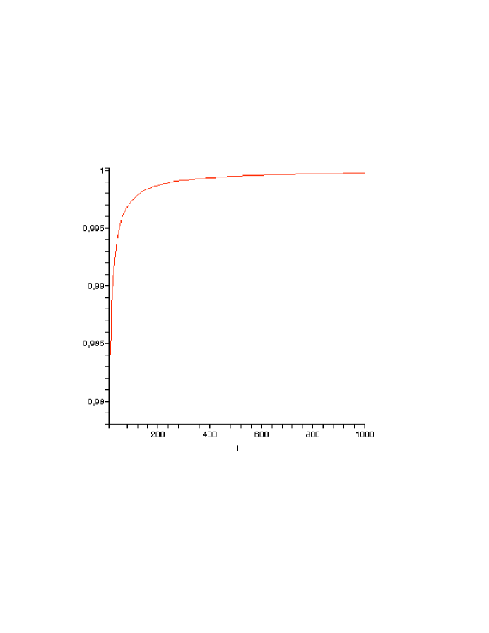
Figure 1: The ratio $R$ as a function of the multipole index $\ell$, for $K=1$

3.2 A stable decomposition

This instability motivates the search for an other decomposition, which is in fact provided by the Maxwell representation . Starting from the multipole expansion (21) of a function $f$, we simply replace each element by its Maxwell representation. This gives the decomposition

$$f_{\leq L}(x)=\left[\lambda_{0}~{}r~{}+~{}\lambda_{1}~{}r^{3}~{}\nabla_{u_{1,1}}+...+\lambda_{\ell}~{}r^{2\ell+1}~{}\nabla_{u_{\ell~{},1}}...\nabla_{u_{\ell~{},\ell}}+...\right.$$

$$\left....+\lambda_{L}~{}r^{2L+1}~{}\nabla_{u_{L~{},1}}...\nabla_{u_{L~{},L}}\right]~{}(\frac{1}{r}),$$ (29)

which is stable by construction. (I thank Jeff Weeks for the idea of this concise demonstration).

3.3 Anisotropy

The multipole vectors offer an immediate advantage: they are rotated by SO(3) as vectors, i.e., according to the usual vector representation. Thus, they seem very appropriate to study the possible anisotropy of the CMB data.

For instance, when $T$ is a Gaussian isotropic random field, all the $T_{(\ell)}$ are independent functions. Thus no correlation should exist between vectors corresponding to different multipole values $\ell$. The situation is not so simple for the different vectors in the decomposition of a given multipole. In the absence of any preferred direction, no peculiar vector could appear in the decomposition. Thus, for any realization, the vectors obtained should be isotropically distributed. For the quadrupole, [4] have studied the algebraic and statistical independences of the coefficients in this decomposition, for a Gaussian random process.

This gives a high significance to the results that CHS and KW report, from their analyses, of an “ astonishing  ” quadrupole and octopole alignment. This clear breaking of isotropy sets the question to interpret it as a chance effect, a contamination of the data, or a cosmological effect. In this latter regard, it is tempting to invoke an universe with multi-connected spatial topology, where the large scale isotropy disappears, and is replaced by partial isotropy, i.e., symmetry under a group $H$ related to the holonomy group $\Gamma$. It is however not so clear that this may explain these results.

It is well known that a multi-connected space imposes a quantification of the wave vectors appearing in the mode decomposition of spatial fluctuations, which is reflected in the distribution of angular temperature fluctuations of the CMB. The statistical distribution of the latter must therefore be invariant under $H$. This has for consequence that, for a given multipole, the distribution of the vector $u_{i}$ must be $H$-invariant, with the immediate consequence that the number of such vectors must be an integer divisor of the order $n_{H}$ of $H$. This implies that, for a perfectly representative distribution, the vectors $u_{i}$ can be present only if $\ell$ (or a divisor of $\ell$) divides $n_{H}$. For instance, if the quadrupole and octopole alignment is significative in this regard, this would imply that $n_{H}$ is a multiple of 6, which puts strong constraints on $H$, and thus on $\Gamma$.

The question of anisotropy has also been treated by [4]. They propose to extract from the set of vectors $u_{i}$ (and the constant $A$) related to a given value of $\ell$, a set of $2\ell-2$ rotation invariant quantities plus 3 rotational degrees of freedom. This interesting suggestion, however, only provides a partial answer to the question of anisotropy. Firstly, the rotation invariant quantities provide information on anisotropy. For example, a multi-connected space will impose some fixed angles between the vectors, in order that the set of vectors be $H$ invariant (for instance, right angles in a toroidal universe). Thus, even if they are rotation invariant, the scalar products between the vectors bring valuable information about anisotropy. On the other hand, the examination of (for instance) the rotation properties of “ anchor vectors ” when $\ell$ increases, has no simple interpretation. For instance, in the simple case of a toroidal universe, the different multipoles (different $\ell$’s) may favor vectors which are the sides, or the diagonals, or different preferred vectors. In this case, despite a strong and well defined anisotropy, the anchor vectors would show no alignment (although they would exhibit some specific and well defined correlations which, however, cannot only be predicted a priori with a specified particular model). Thus we conclude that the interpretation of the multipole vectors in terms of isotropy/anisotropy of the data remains an open question.

In fact (excepted for $\ell=1,2$), there is no standard way to associate to the $\ell$ multipole a definite spatial orientation (which belongs to the 3 dimensional representation of SO(3)). The only exceptions are the dipole ($\ell=1$), which selects one preferred direction; and the quadrupole, which selects a preferred orthonormal frame (see also [2] for an interpretation of the dipole and quadrupole vectors). In fact, an $\ell$ multipole may be seen [3] as a function on the fuzzy (non commutative) sphere $S_{fuzzy,2\ell+1}$, which is itself an approximation of the ordinary sphere by a set of $2\ell+1$ cells.

4 Extension to complex polynomials

The results of CHS and KW were obtained for polynomials, and vectors in the decomposition, with real coefficients. Since, for instance, the usual spherical harmonics correspond to polynomials with complex (not real) coefficients, it seems interesting to try to generalize the previous results. (Note that a basis of real spherical harmonics offers a limited interest, because they are not eigenvectors of the projected angular momentum).

The KW’ s demonstration is based on the existence of $2\ell$ common roots (in $\mathbb{C}P^{2}$), to the two equations $P(X)=0$ and $X^{2}=0$. This remains true when the coefficients of $P(X)$ are complex. However, in this case, the roots are no more two by two complex conjugates. Although a similar demonstration can be performed, there are two main differences :

- it remains true that the $2\ell$ roots can be grouped by pairs, to generate $\ell$ lines. But there is no canonical way to do it, as in the real case (associating the complex conjugates). The consequence is that the resulting decomposition is not unique: there are $N$ different decompositions, $N$ being the number of distinct ways to group the $2\ell$ roots (which may be distinct or not) in pairs.
- In general, the roots are not complex conjugates. Thus the constructed lines are not real. This means that the vectors obtained in the decomposition have complex coefficients.

We obtain thus the following result :

An $\ell$-homogeneous polynomial with complex coefficients, $P\in\mbox{Hom}(\ell)$ can be decomposed in a finite number of different ways, under the form

$$P(X)=\alpha~{}(X\cdot v_{1})...(X\cdot v_{\ell})+X^{2}~{}Q,$$ (30)

where the $v_{i}$ have now complex coefficients and $Q\in\mbox{Hom}(\ell-2)$. Given the normalization constant $\alpha\in\mathbb{C}$, it is not a restriction to assume these vectors unitary ($v^{2}=1$) or null ($v^{2}=0$).

When $P$ has real coefficients, one decomposition (among the others) is canonical, and involves only real (unit) vectors : this is the KW’s result. There are however, in general, other decomposition involving complex vectors, two by two conjugates.

4.1 Some examples

• $P=x^{2}+y^{2}$ has the real decomposition $P=-z^{2}+r^{2}$, but also the complex one $P=(x+iy)(x-iy)$.
  

• $P=x^{2}-y^{2}$ has the real decomposition $P=(x+y)(x-y)$ , but also the complex one $P=-(2y^{2}+z^{2})+r^{2}=-(\sqrt{2}~{}y-iz)(\sqrt{2}~{}y+iz)+r^{2}$.

• For the toy quadrupole of KW, their equation (19), there are, as expected, the 4 roots given by their equation (22). By associating the complex conjugates, they obtained their decomposition (26) with real vectors. But different associations provide the two other decompositions:

  $$1/6[x(1-i\sqrt{2})+3~{}y+z~{}(1-i\sqrt{2})]~{}[x(1+i\sqrt{2})+3~{}y+z~{}(1+i\sqrt{2})]+3r^{2}/2$$

  and

  $$-1/2[-x(1+i\sqrt{2})+y+z~{}(-1+i\sqrt{2})]~{}[x(-1+i\sqrt{2})+y-z~{}(1+i\sqrt{2})]+r^{2}/2.$$

• The toy octopole of KW (27) gives the 6 roots (29,30). The association of the complex conjugates gives the decomposition (32) with real vectors. The different groupings give

  $$(i~{}x+y-z)~{}(-i~{}x+y-z)~{}/2+r^{2}~{}(y-z/2),$$

  and

  $$-(i~{}x+y+z)~{}(-i~{}x+y+z)~{}/2+r^{2}~{}(y+z/2).$$

4.2 The spherical harmonics

Note that the operators $J_{i}\equiv-i\epsilon_{ijk}~{}x^{j}~{}\partial_{k}$, and thus $J^{2}$, commute with $\Delta$ and with $\Pi$. From this, it results that the spherical harmonics are given by

$$Y_{\ell m}=\Pi~{}z^{\ell-m}~{}(x+iy)^{m}.$$ (31)

In particular,
$Y_{\ell\ell}=\Pi~{}~{}(x+iy)^{\ell}=(x+iy)^{\ell},$
$Y_{\ell\ell-1}=\Pi~{}z~{}(x+iy)^{\ell-1}=z~{}(x+iy)^{\ell-1},$
$Y_{\ell\ell-2}=\Pi~{}z^{2}~{}(x+iy)^{\ell-2}=z^{2}~{}(x+iy)^{\ell-1}-r^{2}/3~{}(x+iy)^{\ell-2},$
…
$Y_{\ell 0}=\Pi~{}z^{\ell}=\frac{2^{\ell}~{}(\ell!)^{2}}{(2\ell!)}P_{\ell}(z),$

5 Conclusion

As proven by previous results, the multipole vector decomposition offers a new and promising technique. However, the instability of the decomposition, and the difficulty to interpret anisotropy, clearly demand deeper analysis. In this regard, the result presented here, namely the link with the Maxwell representation, the interpretation in terms of harmonic projection, the established correspondence with the usual harmonic development give some new perspectives.

It remains to analyze the practical relevance of the new stable decomposition proposed here; also, the link between anisotropy and multipole vectors deserves further exploration, in particular in the frame of cosmological models with non trivial topology.

Moreover, the scalar product $X\cdot u$, as a function of $X$, shows some similarities with a wavelet on the sphere. Thus, the multipole vector decomposition shows analogies with a product of wavelets. Since there is presently a lot of interest toward wavelets on the sphere, a further exploration of these analogies may appear fruitful. The construction of a new formalism using the multipole vector decomposition appears therefor as a very promising task.

6 Appendix

By definition, $\Pi(u\cdot X)^{\ell}$, is $\ell-$harmonic and can thus be expanded in spherical harmonics as $\sum_{m}a_{\ell m}(V)~{}Y_{\ell m}(X)$, for $u$ and $X$ on the sphere. Using spherical coordinates, we have

$$X=(\cos\theta,~{}\sin\theta~{}\cos\varphi,\sin\theta~{}\sin\varphi)\mbox{~{}and~{}}u=(\cos\theta^{\prime},~{}\sin\theta^{\prime}~{}\cos\varphi^{\prime},\sin\theta^{\prime}~{}\sin\varphi^{\prime}).$$

Thus, $\Pi(X\cdot u)^{\ell}=\Pi[\cos\theta~{}\cos\theta^{\prime}+\sin\theta~{}\sin\theta^{\prime}~{}\cos(\varphi-\varphi^{\prime})]$ depends on $\varphi^{\prime}$ only through $\varphi-\varphi^{\prime}$. Using $Y_{\ell m}(X)=K_{\ell m}~{}e^{im\varphi}~{}P_{\ell m}(\cos\theta)$, where the $K_{\ell m}$’s are the usual normalization constants and the $P_{\ell m}$’s the Legendre functions, this implies

$$\Pi(X\cdot u)^{\ell}=\sum_{m}F_{\ell m}(\theta^{\prime})~{}e^{-im\varphi^{\prime}}~{}Y_{\ell m}(X)=\sum_{m}F_{\ell m}(\theta^{\prime})~{}e^{im(\varphi-\varphi^{\prime})}~{}K_{\ell m}~{}P_{\ell m}(\cos\theta).$$

By symmetry, we have also

$$\Pi(X\cdot u)^{\ell}=\sum_{m}F_{\ell m}(\theta)~{}e^{im(-\varphi+\varphi^{\prime})}~{}K_{\ell m}~{}P_{\ell m}(\cos\theta^{\prime}).$$

This implies, using symmetry arguments,

$$\Pi(X\cdot u)^{\ell}=K_{\ell}~{}\sum_{m}Y^{*}_{\ell m}(u)~{}Y_{\ell m}(X).$$

The normalization constant

$$K_{\ell}=\frac{4\pi~{}2^{\ell}~{}(\ell!)^{2}}{(2\ell+1)~{}(2\ell!)}$$ (32)

can be calculated from (7), using the polynomial development of $P_{\ell}$.

References

- [1] C.J. Copi, D. Huterer and G.D. Starkman 2003, Multipole vectors — a new representation of the CMB sky and evidence for statistical anisotropy or non-Gaussianity at , submitted to Phys. Rev. D (astro-ph/0310511).
- [2] M R Dennis 2004, Canonical representation of spherical functions: Sylvester s theorem, Maxwell s multipoles and Majorana s sphere, (math-ph/0408046 v1)
- [3] M Lachièze Rey, J-P Gazeau, Eric Huguet , J Renaud and T Garidi, Int. J. Theor. Phys. 2003, vol 42, pp: 1301-1310 (2003), Quantization of the sphere with coherent states (math-ph/0302056)
- [4] K Land and J Magueijo 2004, Multipole invariants and non-Gaussianity, Mon. Not. R. Astron. Soc. (2004), in press (astro-ph/0407081)
- [5] D.J. Schwarz, G.D. Starkman, D. Huterer and C.J. Copi 2004, Is the low- microwave background cosmic?, submitted to Phys. Rev. Lett. (astro-ph/0403353)
- [6] M. Tegmark, A. de Oliveira-Costa and A.J.S. Hamil- ton 2003, A high resolution foreground cleaned CMB map from WMAP, Phys. Rev. D68 (2003) 123523 (astro-ph/0302496)
- [7] Representations of Lie groups and special functions, N. Vilenkin and A. Klimyk, volume 2, Kluwer Academic Publishing, 1993.
- [8] G. Katz and J. Weeks 2004 Polynomial Interpretation of Multipole Vectors, (astro-ph/0405631)