Cosmological Phase Transitions

Abstract

In this lecture at a school for condensed matter physicists, I begin with basic concepts and tools for investigating phase transitions in quantum field theory. The very different roles of global and gauge symmetries in phase transitions will be elucidated. Among the important applications of the basic theory the thermodynamics of the electroweak transition is treated in detail, and the implications for baryogenesis will be discussed. The status of lattice simulations of the transition from a high temperature quark-gluon plasma to confined hadronic matter with spontaneously broken chiral symmetry is also briefly reviewed. The various changes of the free energy density in cosmological phase transitions reinforce the cosmological constant problem. In the last part of the lecture I shall address this profound mystery of present day physics.

1 Introduction

During the evolution of the very early Universe there have been at least two phase transitions. The electroweak theory predicts that at about 100 GeV there was a transition from a ‘symmetric’ high temperature phase with ‘massless’ gauge bosons to the Higgs phase, in which the $SU(2)\times U(1)$ gauge symmetry is ‘spontaneously broken’ and all the masses in the model are generated. A detailed understanding of the nature and dynamics of this transition is a very difficult task, and a lot of quantitative analytical and numerical studies have been performed over the years. One of the motivations of these studies has been that non-perturbative effects might have changed the baryon asymmetry in the phase transition.

Quantum chromodynamics (QCD) predicts that at about 200 MeV there was a transition from a quark-gluon plasma to a confinement phase with no free quarks and gluons. At about the same energy we expect that the global chiral symmetry of QCD with massless fermions is spontaneously broken by the formation of a quark pair condensate. These transitions have been studied extensively in the framework of lattice gauge theory. It is unclear whether they have interesting cosmological implications.

In the framework of unified extensions of the standard model other potentially very interesting phase transitions are expected. In some cases these are accompanied by the formation of topological defects (domain walls, strings, monopoles and textures). This can be cosmologically interesting or dangerous. For example, in a second order phase transition of a grand unified theory (GUT) one expects generically that a completely unacceptable abundance of magnetic monopoles would be formed. This so-called monopole problem was one of the early motivations of inflationary cosmology. The first inflationary model by A.Guth (‘old inflation’) was based on a first order phase transition, and made use of the enormous energy density of the ‘false vacuum’ for the unbroken phase.

These introductory remarks indicate the potential importance of phase transitions in cosmology. In this evening lecture I can, of course, treat only some selected aspects of the subject. Since this is a school for condensed matter physicists, I shall begin with foundational material for investigating phase transitions in quantum field theory. A central tool of most studies is the path integral representation of the partition function. In this connection I want to make some critical remarks about the widespread use of non-convex effective potentials, especially in the older literature, that disturbs me very much. I also want to explain why the roles of global and gauge symmetries in phase transitions are very different. In particular, a gauge symmetry can not be spontaneously broken (Elitzur theorem). As an important application of the basic theory, I shall review existing work on the thermodynamics of the electroweak phase transition, and its role in baryogenesis. We shall continue with a few remarks about the current status of lattice simulations of the QCD phase transitions. The subject of cosmic topological defects that might have been formed in phase transitions will only be touched.

The various changes of the free energy density in cosmological phase transitions reinforces the cosmological constant problem, a deep mystery of present day physics. In the last part of my talk I shall address this topical issue, and then summarize the current evidence for a dominant component of what people (unfortunately) call Dark Energy in our Universe. Whether this is a tiny remainder of an originally huge vacuum energy in the very early Universe remains open, but observations may eventually settle this issue.

2 Phase Transitions in Quantum
Field Theory

Let us first consider a quantum field theory without local symmetries. The partition function can (formally) be represented as an Euclidean path (functional) integral. If $S[\phi]$ denotes the Euclidean action functional of a (multi-component) scalar field $\phi$, say, and if we include the coupling to an external source $J(x)$, this reads

$$Z[J]=\int_{\beta}\exp\{-S[\phi]+(\phi,J)\}~{}[d\phi],$$ (1)

where the integration extends over fields which are periodic in Euclidean time $\tau$, with periodicity $\beta=1/kT$. For textbook treatments see [1] and [2].

Several remarks on this formula are in order. In one dimension, i.e. for quantum mechanics, it has – suitably interpreted – a precise meaning and can be rigorously derived for a large class of interactions. In four dimensions this is rarely the case without an ultraviolet cutoff. An exception are free fields (Gaussian probability measures on spaces of distributions). In perturbation theory, renormalization theory leads – for renormalizable field theories – order by order to meaningful expressions. In some cases, for example for QCD, we expect that the continuum limit of lattice regularizations exists and is physically sound. This is, however, not the case even for simple scalar models (triviality theorem [3]). It is remarkable that this Euclidean formulation in terms of path integrals establishes such a close connection with classical (!) statistical mechanics (models of magnetism). For the study of the thermodynamics of quantum field theories and other issues one can work entirely in the Euclidean framework. An explicit continuation back to Minkowski space is not needed.

An important quantity is $(-\beta)$ times the free Helmholz energy (Schwinger functional):

$$W[J]=\ln~{}Z[J],$$ (2)

that generates the truncated correlation functions. The effective action (Gibbs potential) $\Gamma$ is the generalized Legendre (Legendre-Fenchel) transform of $W[J]$:

$$\Gamma[\Phi]=\sup_{J}\{(\Phi,J)-W[J]\}.$$ (3)

Expectation values of observables $A[\phi]$ are given by

$$\langle A\rangle_{J}=Z[J]^{-1}\int A[\phi]\exp\{-S[\phi]+(\phi,J)\}~{}[d\phi].$$ (4)

$W[J]$ is convex in $J$. For a lattice regularization this follows simply from Hölder’s inequality (see footnote below). Formally, this is implied by

$$\int f(x)\frac{\delta^{2}W[J]}{\delta J(x)\delta J(y)}f(y)d^{4}xd^{4}y=\Bigl{\langle}\Bigl{(}\phi(f)-\langle\phi(f)\rangle\Bigr{)}^{2}\Bigr{\rangle}\geq 0,$$

for every real test function. As a Legendre transform, $\Gamma[\Phi]$ is also convex. For a homogeneous source $J$ the effective potential $V_{eff}(\Phi)$ is, by definition, the free Gibbs energy density.

Consider, for illustration, the simple example of an ‘action’ without a kinetic energy term

$$S[\phi]=\mathcal{U}[\phi]=\int U(\phi)~{}d^{4}x.$$

For $T=0$ and a constant source $J$, the free energy density $w_{0}=W_{0}/\Omega_{4}$ in a finite region of volume $\Omega_{4}$ of a lattice regularization is given by a one-dimensional integral:

$$w_{0}(J)=\frac{1}{\Omega_{4}}\ln\int e^{\Omega_{4}(J\varphi-U(\varphi))}d\varphi.$$ (5)

In the limit $\Omega_{4}\rightarrow\infty$ the Laplace approximation becomes exact, hence

$$w_{0}\rightarrow L(U),$$ (6)

where $L$ denotes the Legendre-Fenchel transformation. This agrees (see Appendix A) with $L$ of the convex hull of $U$, and since $L(L(U))$= convex hull of $U$, we obtain the result that the Gibbs free energy density is for a constant $\Phi$ equal to the convex hull of $U$. In Fig. 1 we show for a non-convex $U$ the transforms $L(U)$ and $L(L(U))$.

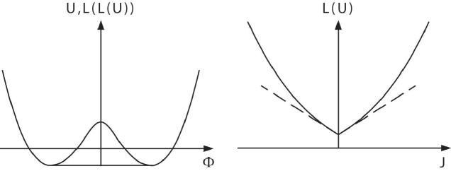
Figure 1: Graphs of a non-convex potential $U$, together with its first and second Legendre-Fenchel transforms.

$L(U)$ is still the free energy density for $T>0$. (Note that for $T>0$ the volume $\Omega_{4}$ is $\beta$ times the three-volume $\Omega_{3}$.)

Phase transitions

In Figs. 2 and 3 we show the typical shapes of effective potentials for first and second order phase transitions. Their Legendre-Fenchel transformations are the Helmholtz free energy densities. The reader is invited to sketch these. For instance, the slope of $w(J)$ corresponding to Fig. 2 develops for $T\downarrow T_{c}$ and $J=0$ a jump (discontinuity in the ‘magnetization’), while for Fig. 3 the ‘magnetization’ vanishes at $T\geq T_{c}$ and starts to grow below $T_{c}$.

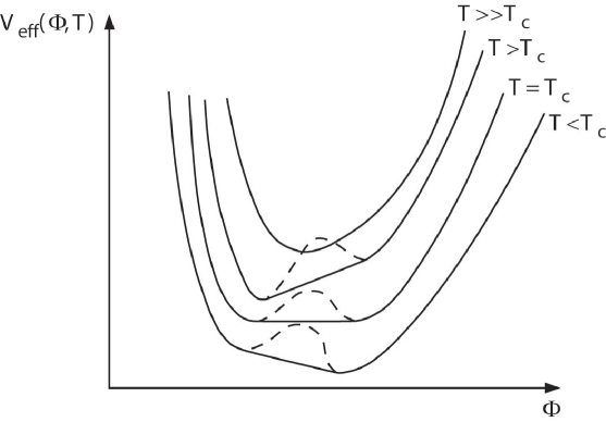
Figure 2: Effective potential for a first order phase transition. At the critical temperature the minimum is degenerate (horizontal line corresponds to a phase mixture). The order parameter makes a jump between the pure phases.

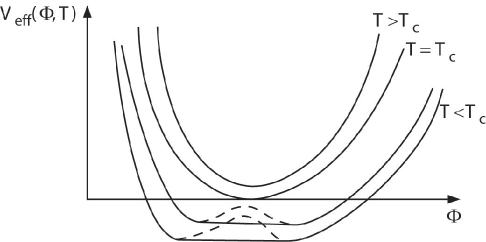
Figure 3: Effective potential for a second order phase transition. For the critical temperature the second derivative vanishes at the minimum. The horizontal straight line below $T_{c}$ shrinks to a point at $T_{c}$.

Footnote: Convexity of $W[J]$

The convexity of $W[J]$ holds even in a finite volume, and not only in the thermodynamic limit. (Actually, $W$ is then even strictly convex). The lattice regularized partition sum is then an integral of the form

$$Z(\mbox{\boldmath$\alpha$})=\int\exp\Bigl{(}\mbox{\boldmath$\alpha\cdot f$}(x)\Bigr{)}d\mu(x),$$

where $\alpha$=$(\alpha_{1},...,\alpha_{k})$ and $\alpha\cdot f$$(x)=\sum\alpha_{i}f_{i}(x)$. We claim that for any $\lambda$ with $0<\lambda<1$

$$\ln Z\Bigl{(}\lambda\mbox{\boldmath$\alpha$}+(1-\lambda)\mbox{\boldmath$\beta$}\Bigr{)}\leq\lambda\ln Z(\mbox{\boldmath$\alpha$})+(1-\lambda)\ln Z(\mbox{\boldmath$\beta$}).$$

This follows from the following application of Hölder’s inequality

$$\|FG\|_{1}\leq\|F\|_{p}\|G\|_{q},~{}~{}~{}\frac{1}{p}+\frac{1}{q}=1~{}~{}(p>1),$$

for $F=e^{\lambda f},~{}G=e^{(1-\lambda)g},~{}p=1/\lambda,~{}q=1/(1-\lambda),~{}e^{f}\in L^{1}(\mu)$.

Usually, the convexity of $\ln Z$ is established by considering the quadratic form

$$\frac{\partial^{2}\ln Z}{\partial\alpha_{i}\partial\alpha_{j}}\xi_{i}\xi_{j}=\langle(f_{\xi}-\langle f_{\xi}\rangle)^{2}\rangle\geq 0,$$

where $f_{\xi}:=\sum_{i}f_{i}\xi_{i}$, and the angular bracket denotes the expectation value with respect to the probability measure $Z(\mbox{\boldmath$\alpha$})^{-1}\exp\Bigl{(}\mbox{\boldmath$\alpha\cdot f$}\Bigr{)}d\mu$.

This argument shows that $\ln Z$ is convex as a function of any parameter that appears linearly in the exponential under the integral sign in $Z$.

2.1 Mean field approximation

Countless expressions and plots in books and articles violate the basic convexity property, usually as a result of some approximate calculations that are analytically extended to regions where they are no more valid. Even in some really good books that happens already for the mean field approximation. For illustration let me explain what is not done properly.

Consider a one component neutral scalar field with Euclidean action in $D$ dimensions

$$S[\phi]=\int\Bigl{[}\frac{1}{2}(\partial\phi)^{2}+U(\phi)\Bigr{]}~{}d^{D}x\equiv T[\phi]+\mathcal{U}[\phi].$$ (7)

To have well-defined expressions interpret all the formulae in the lattice regularization for finite (hypercube) subsets $\Lambda$ of the lattice. (Then $T[\phi]$ contains nearest neighbor interactions.) Beside the action $S$ we consider an ‘approximate’ action $S_{0}$ and the corresponding probability measures

$$d\mu_{0}(\phi)=Z_{o}^{-1}e^{-S_{0}}[d\phi],~{}~{}~{}Z_{0}=\int e^{-S_{0}}[d\phi]$$ (8)

for all finite subsets $\Lambda$. The corresponding expectation values are denoted by $\langle A\rangle_{0}$. The starting point is Jensen’s inequality

$$\langle\exp A\rangle_{0}\geq\exp(\langle A\rangle_{0})$$ (9)

for $A=-S+(\phi,J)+S_{0}$, and for $S_{0}$ we choose

$$S_{0}=-(\phi,K)+\mathcal{U}[\phi],$$ (10)

where $K(x)$ is another external source. This gives, if $W_{0}=\ln~{}Z_{0}$,

$$W[J]\geq W_{0}+\langle S_{0}-S+(\phi,J)\rangle_{0}=W_{0}[K]-\langle T[\phi]\rangle_{0}+((J-K),\langle\phi\rangle_{0}).$$ (11)

For $\overline{\phi}:=\langle\phi\rangle_{0}$ we have

$$\overline{\phi}(x)=\frac{\partial W_{0}[K]}{\partial K(x)}.$$ (12)

Since $\langle\phi(x)\phi(y)\rangle_{0}=\langle\phi\rangle_{0}\langle\phi(y)\rangle_{0}$, we find

$$W[J]\geq\mathcal{W}[J,K]:=W_{0}[K]-T[\overline{\phi})]+((J-K),\overline{\phi}).$$ (13)

The mean field free energy $W_{mf}[J]$ is the supremum in $K$ of the Landau functional $\mathcal{W}[J,K]$, often also called the Landau free energy. Since $W_{0}[K]$ is convex, $K$ and $\overline{\phi}$ are according to (12) in one to one correspondence. Hence we can write

$$W_{mf}[J]=\sup_{\overline{\phi}}\{(\overline{\phi},J)-(\Gamma_{0}[\overline{\phi}]+T[\overline{\phi}])\},$$ (14)

where $\Gamma_{0}$ is the Legendre transform of $W_{0}$. This equation shows that $W_{mf}[J]$ is the Legendre-Fenchel transform of $\Gamma_{0}[\overline{\phi}]+T[\overline{\phi}]$, and is therefore convex. Furthermore (see Appendix A), the mean free Gibbs potential is given by

$$\Gamma_{mf}[\Phi]=convex~{}hull~{}\{\Gamma_{0}[\Phi]+T[\Phi]\}.$$ (15)

It is crucial that this is convex. Most authors work with the standard Legendre transform and end up for $\Gamma_{mf}$ with the functional in the curly bracket, which is in general not convex. (For a typical example, see Figs. 24.1, 2 in [4].) Note also that the Landau functional, expressed as a function of $J$ and $\overline{\phi}$, is given by the curly bracket in (14)

$$\mathcal{W}[J,\overline{\phi}]=(J,\overline{\phi})-(\Gamma_{0}[\overline{\phi}]+T[\overline{\phi}]).$$ (16)

For $J=0$ its convex hull is according to (15) equal to $-\Gamma_{mf}$. We emphasize that the Landau functional is in general not convex.

As an exercise, one may work out everything for the Ising model.

2.2 One-loop approximation

The loop expansion of the Gibbs free energy $\Gamma[\Phi]$ is a much used systematic approximation scheme. We recall here only the zero- and one-loop terms. These are obtained with the steepest decent method.

The saddle points $\phi_{0}$ of the exponent in (1) satisfy the classical equation of motion

$$\left.\frac{\delta S}{\delta\phi}\right|_{\phi_{0}}=J.$$

Let us first assume that there is only one such saddle point for a given $J$. This is, for instance, the case for an action of the form (7) for a convex potential $U(\phi)$, because the previous equation then becomes

$$-\Delta\phi_{0}+U^{\prime}(\phi_{0})=J,$$

which has at most one solution if $J(x)$ vanishes at infinity and $\phi_{0}$ is assumed to go to zero at infinity. In the expansion

$$S[\phi]-(\phi,J)=S(\phi_{0})-(\phi_{0},J)+\frac{1}{2}(\psi,A\psi)+...,$$

with $\psi:=\phi-\phi_{0}$, and

$$A(x,y)=\left.\frac{\delta^{2}S}{\delta\phi(x)\delta\phi(y)}\right|_{\phi_{0}},$$ (17)

we leave out the higher orders and arrive at

$$Z[J]\simeq\exp\{(\phi,J)-S[\phi_{0}]\}\int e^{-\frac{1}{2}(\psi,A\psi)}[d\psi].$$ (18)

We interpret all the formulas in the lattice regularization (for a finite sublattice). The leading order of $W[J]$ is given by the Laplace approximation

$$W_{0}[J]=(\phi_{0},J)-S[\phi_{0}]=(LS)[J].$$ (19)

Therefore, the leading order $\Gamma_{0}$ of $\Gamma$ is given by

$$\Gamma_{0}[\Phi]=S[\Phi]$$ (20)

(‘Landau approximation’). The one-loop correction is determined by the Gaussian integral

$$\int e^{-\frac{1}{2}(\psi,A\psi)}[d\psi]=\Bigl{(}\det\frac{A}{2\pi}\Bigr{)}^{-\frac{1}{2}}.$$

For $W[J]$ we arrive at

$$W[J]=W_{0}[J]+W_{1}[J]+...~{},~{}~{}~{}W_{1}[J]=-\frac{1}{2}\ln\det\Bigl{(}\frac{A}{2\pi}\Bigr{)}.$$ (21)

For a given $J$ the conjugate variable $\Phi$ differs from the classical solution $\phi_{0}$ by a first order quantity. Up to second order we can thus replace $\phi_{0}$ by $\Phi$ in the expression (21) for $W_{1}$. Therefore, the Legendre transformation (3)

$$\Gamma[\Phi]=\sup_{J}\{(\Phi,J)-LS[J]-W_{1}[\phi_{0}(J)]+...\}$$

is given by

$$\Gamma[\Phi]=\Gamma_{0}[\Phi]+\Gamma_{1}[\Phi]+...~{},~{}~{}~{}\Gamma_{1}[\Phi]=\frac{1}{2}\ln\det\Bigl{(}\frac{A}{2\pi}\Bigr{)},$$ (22)

where $A$ is now the expression (17) at $\phi=\Phi$.

If we set in (7) $U(\phi)=\frac{1}{2}m^{2}\phi^{2}+P(\phi)$, where $P(\phi)$ is a polynomial (of degree $\leq 4$ for renormalizable interactions), then the 1-loop contribution of $\Gamma(\Phi)$ is given by the following expression (up to $\Phi$ and $T$ independent terms)

$$\Gamma_{1}(\beta,\Phi)=\frac{1}{2}\ln\det\left\{\frac{1}{2\pi}\left[-\Delta+m^{2}+P^{\prime\prime}(\Phi)\right]\right\}.$$ (23)

The temperature dependence is contained in the Laplacian (periodicity in the Euclidean time direction). The functional determinant can be worked out formally in the continuum theory or from the lattice regularization, for which it is well-defined and can easily be computed using Fourier transformation on a finite lattice. The details are given in Appendix B, where we also show that the continuum limit of the temperature dependent part $V_{1}(\beta,\Phi)$ of the effective potential (free energy density) exists, and is given by

$$V_{1}(\beta,\Phi)=\frac{1}{\beta}\int\frac{d^{3}k}{(2\pi)^{3}}\ln\Bigl{(}1-e^{-\beta\Omega(k)}\Bigr{)},$$ (24)

where

$$\Omega(k)=\sqrt{k^{2}+M^{2}},~{}~{}~{}M^{2}:=m^{2}+P^{\prime\prime}(\Phi).$$ (25)

The reader is invited to generalize this to the grand canonical ensemble of a complex scalar field.

The $T=0$ contribution requires renormalizations. As a starting point we use the lattice regularization, derived in Appendix B. According to (63) we obtain in the thermodynamic limit for an x-independent $\Phi$

$$\lim\frac{1}{\Omega_{4}}\ln\det\left[-\Delta+M^{2}\right]=\int_{BZ}\frac{d^{4}k}{(2\pi)^{4}}\ln\Bigl{[}M^{2}+\frac{2}{a^{2}}\sum_{\alpha}(1-\cos k_{\alpha}a)\Bigr{]},$$ (26)

where the integral now extends over the four-dimensional Brillouin zone $BZ=[-\frac{\pi}{a},\frac{\pi}{a}]^{4}$. In what follows it is simpler to use a spherical cut-off $k^{2}\leq\Lambda^{2}$. In the continuum limit $a\rightarrow 0$ we find for the regularized one-loop effective potential $V_{1}(\Phi)$ at $T=0$, up to $\Phi$-independent contributions,

$$V_{1}^{\Lambda}(\Phi)=\frac{1}{2}\int_{k^{2}\leq\Lambda^{2}}\ln\left[\frac{k^{2}+V_{0}^{\prime\prime}(\Phi)}{\mu^{2}}\right]\frac{d^{4}k}{(2\pi)^{4}}$$ (27)

$(V_{0}=U)$, where we have introduced an arbitrary mass scale $\mu$ (leading to a change of $V_{1}$ which is independent of $\Phi$). This can be written as

$$V_{1}(\Phi)=\frac{\mu^{4}}{32\pi^{2}}f(V_{0}^{\prime\prime}/\mu^{2}),$$

with

$$f(y)=\int_{0}^{\Lambda/\mu}\ln(x+y)x~{}dx.$$

We note that the third derivative of $f$ is given by

$$f^{\prime\prime\prime}(y)=\int_{0}^{\Lambda/\mu}\frac{2x}{(x+y)^{3}}~{}dx$$

and converges for $\Lambda\rightarrow\infty$ to $1/y$. Hence, $f(y)=\frac{1}{2}y^{2}\ln(y)$ + quadratic polynomial in $y$. So,

$$V_{1}(\Phi)=\frac{1}{64\pi^{2}}(V_{0}^{\prime\prime})^{2}\ln\left(\frac{V_{0}^{\prime\prime}}{\mu^{2}}\right)+\mbox{quadratic polynomial in}~{}V_{0}^{\prime\prime}/\mu^{2}.$$

The second order polynomial can be compensated by a renormalization of the coupling constants in $V_{0}=U$. Note that we also have to renormalize a $\Phi$-independent vacuum energy. This will become a crucial issue when gravity is included (see Sect. 4).

After renormalization the effective potential for $T=0$ is, up to one loop, given by

$$V_{eff}(\Phi)=V_{0}(\Phi)+\frac{1}{64\pi^{2}}\Bigl{[}V_{0}^{\prime\prime}(\Phi)\Bigr{]}^{2}~{}\ln\Bigl{[}V_{0}^{\prime\prime}(\Phi)/\mu^{2}\Bigr{]}.$$ (28)

Remark. A change of the scale $\mu^{2},~{}\mu^{2}\rightarrow e^{t}\mu^{2}$, can be absorbed by a change of the coupling constants in $V_{0}(\Phi;p(t))$, where the parameters $p(t)$ satisfy, up to higher orders, the differential equation

$$\frac{d}{dt}V_{0}(\Phi;p(t))=\frac{1}{64\pi^{2}}\Bigl{[}V_{0}^{\prime\prime}(\Phi:p(t))\Bigr{]}^{2}.$$

If

$$V_{0}(\varphi)=h+k\varphi+\frac{m^{2}}{2!}\varphi^{2}+\frac{f}{3!}\varphi^{3}+\frac{g}{4!}\varphi^{4},$$

we obtain for $t=0$ the renormalization group equation

$$\frac{dg}{dt}=\frac{3}{32\pi^{2}}g^{2},~{}~{}~{}\mbox{etc.}$$ (29)

Convex potentials

For a convex potential like $U(\phi)=\frac{1}{2}m^{2}\phi^{2}+\frac{\lambda}{4}\phi^{4}$, $M^{2}(\Phi)=m^{2}+3\lambda\Phi^{2}$ is positive, and the one-loop effective potential is convex. The minimum occurs at $\Phi=0$, and in this symmetric phase the T-dependent effective mass is

$$m^{2}(T)=m^{2}+\left.\frac{\partial^{2}V_{1}(\beta,\Phi)}{\partial\Phi^{2}}\right|_{\Phi=0}.$$ (30)

The T-dependent term can be read off from (24)

$$\left.\frac{\partial^{2}V_{1}(\beta,\Phi)}{\partial\Phi^{2}}\right|_{\Phi=0}=3\lambda\int\frac{d^{3}k}{(2\pi)^{3}}\frac{1}{\omega}\frac{1}{e^{\beta\omega}-1},~{}~{}~{}\omega=\sqrt{k^{2}+m^{2}}.$$ (31)

For high temperatures we have

$$m^{2}(T)=m^{2}+\frac{1}{4}\lambda\Bigl{[}T^{2}-\frac{3}{4\pi}mT+\mathcal{O}(m^{2}\ln(m^{2}/T^{2}))\Bigr{]}.$$ (32)

For $m=0$ the scalar field acquires a mass $\sqrt{\lambda}T/2$ which plays the role of an infrared cutoff.

Problems with non-convex potentials

For a non-convex potential $U$ (with the ‘wrong’ sign of the mass term) we can not simply use the previous formulae, since $M^{2}(\Phi)$ becomes negative for small $\Phi$, whence $V_{1}(\beta,\Phi)$ in (24) becomes complex. This means that the one-loop potential is not valid for small arguments, that are of particular interest in studies of the early universe. What should one do in this situation? We shall address this question below.

For a rough estimate of the critical temperature for the transition to the symmetric phase we may naively ignore this and use the leading corrections in (32):

$$m^{2}(T_{c})=0\simeq m^{2}+\frac{1}{4}\lambda T_{c}^{2}.$$ (33)

This gives (Kizhnit, Linde, Weinberg)

$$T_{c}^{2}\simeq\frac{(-4m^{2})}{\lambda}~{}~{}~{}(m^{2}<0).$$ (34)

For weak coupling this implies that $T_{c}^{2}\gg-m^{2}$, and we can therefore expect that (34) is a good estimate.

The unrenormalized parameter $m^{2}$ in this equation can be replaced by the mass of the physical particle (the “$\sigma$ meson”). In lowest order, $m_{\sigma}^{2}=-2m^{2}$, hence

$$T_{c}^{2}=\frac{2m_{\sigma}^{2}}{\lambda}.$$ (35)

We can, however, not ignore the encountered problems with the one-loop effective potential. It is quite clear that the saddle point approximation can only hold near the minima. If there are, for example, two similarly deep minima, as is expected close to the critical temperature, one has to take both into account. As a recipe one might take the convex hull of the sum of the saddle point approximations for the two minima. But this is just a reasonable recipe. Another approach was studied in [5], where the standard definition of the effective potential is modified by coupling the source to a quadratic polynomial of the scalar field. The new potential is not necessarily convex as a function of the average value of $\phi$, but is convex as a function of the composite field since this is the conjugate variable. The modified potential closely tracks the usual one where the latter is real. Moreover, at finite temperatures it displays a local minimum at $\Phi=0$. It is also worthwhile to note that the resulting critical temperature in the one-loop approximation confirms the rough estimate (34).

2.3 The constraint potential

We consider now the free energy for a given spatial average of the order parameter. For simplicity, we do this for a scalar field theory, since generalizations are obvious. As before, the formulae below are well-defined in the lattice regularization. For a finite region $\Lambda$ we sample the field configurations according to their mean field

$$\bar{\phi}=\frac{1}{\left|\Lambda\right|}\int\phi~{}d^{D}x.$$

The probability distribution of $\bar{\phi}$ for a homogeneous source $J$ is given by

$$dP(\bar{\phi}) = \left\langle\delta\Bigl{(}\bar{\phi}-\frac{1}{\left|\Lambda\right|}\int\phi~{}d^{D}x\Bigr{)}\right\rangle d\bar{\phi}$$

$$= e^{J\left|\Lambda\right|\bar{\phi}}d\bar{\phi}~{}Z_{\Lambda}(J)^{-1}\int e^{-S_{\Lambda}[\phi]}\delta\Bigl{(}\bar{\phi}-\frac{1}{\left|\Lambda\right|}\int\phi~{}d^{D}x\Bigr{)}[d\phi]_{\Lambda}$$

$$\equiv \frac{1}{Z_{\Lambda}(J)}\exp\Bigl{(}\left|\Lambda\right|[J\bar{\phi}-V_{c}(\bar{\phi})]\Bigr{)}d\bar{\phi}.$$

The constraint potential $V_{c}$ (which depends on $\Lambda$) is given in terms of the integral in the last equation as

$$e^{-\left|\Lambda\right|V_{c}(\bar{\phi})}=\int e^{-S_{\Lambda}[\phi]}\delta\Bigl{(}\bar{\phi}-\frac{1}{\left|\Lambda\right|}\int\phi~{}d^{D}x\Bigr{)}[d\phi]_{\Lambda}.$$ (36)

Since $dP$ is a probability measure, we have

$$Z_{\Lambda}(J)=\int e^{\left|\Lambda\right|[J\bar{\phi}-V_{c}(\bar{\phi})]}d\bar{\phi}.$$ (37)

In other words, $W_{\Lambda}(j)$ is obtained from $V_{c}$ by a Laplace transformation. For finite regions $V_{c}$ is usually not convex.

In the infinite volume limit the Laplace approximation again becomes exact if the saddle point of $V_{c}-J\bar{\phi}$ is unique in this limit. Hence

$$\frac{1}{\left|\Lambda\right|}W_{\Lambda}(J)\rightarrow w(J)=\sup_{\bar{\phi}}[J\bar{\phi}-V_{c}(\bar{\phi})]=(LV_{c})(J),$$ (38)

which implies that the effective potential is equal to the convex hull of the thermodynamic limit of the constraint potential. Since it can be shown [10] that the latter is convex (certainly if the saddle point is unique, but presumably in general), the two potentials must be the same in this case.

Note that for $J=0$ the probability density $p(\bar{\phi})$ to find the system in a state of ‘magnetization’ $\bar{\phi}$ is given by

$$p(\bar{\phi})=e^{-\left|\Lambda\right|V_{c}(\bar{\phi})}\left[\int e^{-\left|\Lambda\right|V_{c}(\bar{\phi})}d\bar{\phi}\right]^{-1}.$$

The constraint effective potential has thus a very intuitive meaning. It has often been studied via lattice simulations. For an example of an interesting recent application (vacuum stability), see [11].

2.4 Effective potential for gauge theories

For gauge theories it is advisable to construct a gauge invariant effective potential, that has a physical interpretation in terms of a gauge invariant order parameter. In this context it has to be stressed that for lattice regularizations of locally symmetric field theories any local quantity which is not gauge invariant, and has no gauge invariant component (for precisions, see Appendix C), such as a Higgs field, has a vanishing expectation value at any temperature. In this sense gauge invariance can not be spontaneously broken (Elitzur theorem [6]). In perturbation theory, where one expands about a Gaussian measure, this is not so because gauge invariance is explicitly broken by gauge fixing. In the lattice formulation one does, however, not have to fix a gauge. (In practice, it may be useful to fix the gauge if the ensemble of configurations is not very large.)

Lattice formulation of gauge theories

The lattice regularization of gauge theories (Wilson) is of crucial importance in the strong (confined) field regime, because there is no other way to perform numerical calculations. But also from the conceptual point of view, lattice gauge theories are very interesting. For systematic presentations, see [7] and [8].

In this discrete formulation of a gauge theory, belonging to a compact group $G$, the gauge potential is replaced by a map of bonds (ordered pairs $b$ of nearest neighbor lattice points) into $G$: $b\mapsto g_{b}\in G$, with the property that $g_{x,y}=g_{y,x}^{-1}$ for any bond $b=\langle x,y\rangle$. In order to formulate the analog of the Yang-Mills action we need the notion of a plaquette. This is a closed curve of four bonds $P={\langle x,y\rangle,\langle y,z\rangle,\langle z,u\rangle\langle u,x\rangle}$. To each of these we assign the group element $g_{\partial P}=g_{x,y}g_{y,z}g_{z,u}g_{u,x}$, and for a given unitary character $\chi$ of the group $G$ the real number

$$S_{P}=\frac{1}{2}\Bigl{(}\chi(g_{\partial P)}+\chi^{*}(g_{\partial P})\Bigr{)}.$$ (39)

Note that $S_{P}$ is independent of the orientation of $P$. More generally, we can assign to each closed path $\mathcal{C}$ on the lattice the product $g_{\mathcal{C}}$ of its $g_{b}$’s, along one of the orientations, and then take its character $\chi(\mathcal{C})$. This number is also independent of which site we begin the loop with. The action of a configuration $\{g\}$ on a finite region $\Lambda$ of the lattice is taken to be

$$S_{\Lambda}({g})=-\sum_{P\subset\Lambda}S_{P}.$$ (40)

The expectation value of an ‘observable’ $A(\{g\})$ in $\Lambda$ is defined by

$$\langle A\rangle_{\Lambda}=\frac{1}{Z_{\Lambda}}\int\exp(-S_{\Lambda})A~{}d\mu_{\Lambda},~{}~{}~{}Z_{\Lambda}=\int e^{-S_{\Lambda}}~{}d\mu_{\Lambda},$$ (41)

where $d\mu_{\Lambda}$ is the product of the normalized Haar measures for all bonds in $\Lambda$.

A local gauge transformation is a map $x\mapsto\gamma_{x}\in G$. Under such a transformation a gauge field configuration transforms as

$$g_{x,y}\mapsto\gamma_{x}g_{x,y}\gamma_{y}^{-1}~{}~{}~{}(b=\langle x,y\rangle).$$ (42)

Clearly, $S_{P}$, the action and the measures $d\mu_{\Lambda}$ are invariant under local gauge transformations.

Using the Baker-Hausdorff formula, it is easy to see that the naive formal continuum limit leads to the Yang-Mills theory. There are good reasons to believe that the continuum limit of a pure lattice gauge theory provides a consistent interacting Euclidean field theory.

Next, we add in a gauge invariant manner Higgs fields to the lattice model. To do this for such a field $\phi(x)$, we have first to introduce a discrete form of the covariant derivative. If this field transforms with respect to $G$ according to the unitary representation $U(g)$, then the following definition has the right formal continuum limit (we use the notation introduced in Appendix B)

$$D_{\mu}\phi(x)=\frac{1}{a}\Bigl{[}U(g_{x,x+ae_{\mu}})\phi(x+ae_{\mu})-\phi(x)\Bigr{]}.$$ (43)

The adjoint operator is

$$D_{\mu}^{\dagger}\phi(x)=\frac{1}{a}\Bigl{[}U(g_{x,x-ae_{\mu}})\phi(x-ae_{\mu})-\phi(x)\Bigr{]}.$$ (44)

The corresponding gauge invariant Laplace operator (generalizing (57) in Appendix B) is

$$\Delta_{\{g\}}=-D_{\mu}^{\dagger}D_{\mu}.$$ (45)

The discrete Higgs part of the action is then in $D$ dimensions (dropping the $\Lambda$-dependence)

$$S^{H}[\{g\},\phi]=\frac{1}{2}a^{D-2}\sum_{\langle x,y\rangle}\mid U_{x,y}\phi(y)-\phi(x)\mid^{2}+a^{D}\sum_{x}V(\phi(x)),$$ (46)

where $U_{x,y}:=U(g_{x,y})$.

When fermionic fields are discretized in the most obvious way, the problem of ‘fermion doubling’ shows up. Early remedies to cure this involved an explicit breaking of chiral symmetry of QCD (see, e.g., Chap. 4 of [8]). Fortunately, there has been recently important progress in solving this long-standing problem. Lattice formulations that preserve chiral symmetry have been found, but in practice numerical simulations become much harder. For a very readable recent review on these aspects, see [9].

Continuum limit

What we are really interested in is what the theory describes in the continuum limit. The lattice is only used as an ultraviolet gauge invariant regularization, valid outside the domain of perturbation theory.

Consider, for concreteness, a pure Yang-Mills lattice theory with a single dimensionless (bare) coupling constant $g$. The only dimensionful parameter in the theory is the lattice spacing $a$. Therefore, a physical quantity with the dimension of a mass, say, such as a particle mass $m_{phys}$, must be of the form

$$m_{phys}=\frac{1}{a}f(g).$$

The theory allows us to compute $f(g)$, and thus ratios of masses. Clearly, in taking the continuum limit $a\rightarrow 0$ we have to tune $g$ as a function of $a$ such that $am_{phys}\rightarrow 0$. Since the inverse, $\xi=(am_{phys})^{-1}$, is a correlation length, we have to approach – in the language of statistical mechanics – a critical point of the theory. The tuning of $g(a)$ is controlled by a renormalization group equation of the form

$$a\frac{dg}{da}=-\beta_{LAT}(g).$$

In lattice perturbation theory $\beta_{LAT}(g)$ can be computed as a power series in $g$ for small $g$:

$$\beta(g)=-\beta_{0}g^{3}-\beta_{1}g^{5}+....$$

For $SU(N)$ one finds

$$\beta_{0}=\frac{N}{16\pi^{2}}\frac{11}{3},~{}etc.$$

From this we find by integration

$$g^{2}=-\frac{1}{\beta_{0}\ln(a^{2}\Lambda_{LAT}^{2})}+...~{},$$

where $\Lambda_{LAT}$ is an integration constant. Inverting this one sees that

$$am_{phys}=const~{}\exp\Bigl{(}-\frac{1}{2\beta_{0}g^{2}}\Bigr{)}\cdot(...),$$

showing the non-perturbative character of masses in the theory. Note that the bare coupling constant $g(a)$ vanishes in the continuum limit.

The dimensionful lattice $\Lambda$-parameter, $\Lambda_{LAT}$, provides a scale which survives the continuum limit. This is remarkable, because classically the theory has no scale. Through the process of renormalization we have introduced a mass scale into the quantized theory, a mechanism that is often called dimensional transmutation. This renormalization procedure is in the lattice formulation no more mysterious than adjusting the temperature toward the Curie point of a ferromagnet. At the same time these considerations shows that the continuum limit has to be taken with care. They also show an interesting point of contact with critical behavior, discussed in other lectures at this school.

Elitzur’s theorem for gauge theories

For systems with global symmetries the phenomenon of spontaneous symmetry breaking (SSB) is well-known. This is accompanied by a non-vanishing ‘magnetization’. At first sight one expects something similar for gauge theories. However, Elitzur [6] has shown that local quantities, like the bond variables $g_{b}$ or a Higgs field, which are not gauge invariant, have always vanishing mean values. This is quite easy to prove, and is also physically understandable. It is instructive to show this first for a lattice gauge theory with gauge group $Z_{2}$, because this shows the contrast to the Ising model. In Appendix C we give a general proof of Elitzur’s theorem.

The bond variables will be denoted by $\sigma_{b}(=\pm 1$. The action for a finite region $\Lambda$ of the lattice $Z^{D}$ is taken to be

$$S_{\Lambda}(\{\sigma\})=-\sum_{P\subset\Lambda}\sigma_{\partial P}-h\sum_{b\subset\Lambda}\sigma_{b},$$ (47)

where $h$ is an external ‘field’. We could also include a Higgs field $\phi_{i}$, transforming according to $\phi_{i}\mapsto\varepsilon_{i}\phi_{i},~{}\varepsilon_{i}=\pm 1$.

Before continuing with this model, let us recall the SSB for the Ising model with its global symmetry $Z_{2}$, consisting of the identity and the reflection $\sigma_{i}\mapsto-\sigma_{i}$ for the Ising spins $\sigma_{i}$ of all lattice sites $i$. Above a critical temperature $T_{c}$ there is only one infinite-volume equilibrium (Gibbs) state. However, for $T<T_{c}$ each translation invariant equilibrium state (probability measure) $\mu^{\beta}$ is a convex linear combination of two different extremal states $\mu_{\pm}^{\beta}$. This means that $\mu^{\beta}$ describes a mixture of two pure phases. The probability measures $\mu_{\pm}^{\beta}$ are weak limits of Gibbs states on finite regions $\Lambda\subset Z^{D}$ with $\pm$ boundary conditions outside $\Lambda$. Since they are different, they are not invariant under the symmetry group $Z_{2}$ of the interaction; the symmetry is spontaneously broken for these pure phases. Correspondingly, the spontaneous magnetizations

$$m_{\pm}(\beta)=\langle\sigma_{i}\rangle_{\mu_{\pm}^{\beta}}$$ (48)

do not vanish for $\beta>\beta_{c}$.

In sharp contrast to this situation, the mean value of $\langle\sigma_{b}\rangle$ does not signal a symmetry breaking for the $Z_{2}$ lattice gauge model:

Theorem (Elitzur). For the expectation value $\langle\sigma_{b}\rangle_{\Lambda}(h)$ we have

$$\lim_{h\downarrow 0}\langle\sigma_{b}\rangle=0~{}~{}~{}\mbox{{uniformly in} $\Lambda$ {and} $\beta$}.$$ (49)

In particular, the thermodynamic limit of $\langle\sigma_{b}\rangle_{\Lambda}(h)$ vanishes for $h\downarrow 0$ (no spontaneous ‘magnetization’).

Before giving the simple proof, we remark that when a Higgs field $\phi_{x}$ is added, a similar proof shows that

$$\langle\phi_{x}\rangle=0$$ (50)

(Exercise). This does, however, not exclude a Higgs phase with an exponential fall off of the truncated correlation function $\langle\sigma_{\partial P_{1}}\sigma_{\partial P_{2}}\rangle_{c}$ for the gauge fields (mass generation), but (49) and (50) show that this is not signaled by local gauge variant observables. This fact is well-known to people working in lattice gauge theory, but is largely ignored outside this community. As order parameters one may try to choose local gauge invariant quantities, such as the norm of a Higgs field.

Proof of Elitzur’s theorem.  We can choose in (46) the bond variable $\sigma_{01}$ for the bond $b=\langle 0,1\rangle$, and estimate in

$$\langle\sigma_{01}\rangle_{\Lambda}=\frac{\sum_{\{\sigma\}}\sigma_{01}\exp(\beta\sum_{P}\sigma_{\partial P}+\beta h\sum_{b}\sigma_{b})}{\sum_{\{\sigma\}}\exp(\beta\sum_{P}\sigma_{\partial P}+\beta h\sum_{b}\sigma_{b})}$$ (51)

the numerator $N$ and the denominator $D$ separately.

Consider a gauge transformation $\sigma_{ij}^{\prime}=\varepsilon_{i}\sigma_{ij}\varepsilon_{j}$, with $\varepsilon_{i}=1$ for $i\neq 0$ and replace $\sigma_{ij}$ in $N$ and $D$ by $\varepsilon_{i}\sigma_{ij}^{\prime}\varepsilon_{j}$, dropping afterwards the prime of $\sigma_{ij}~{}(\sigma_{ij}\mapsto\varepsilon_{i}\sigma_{ij}\varepsilon_{j})$. This can be done for $\varepsilon_{0}=\pm 1$. $D$ is equal to half the sum:

$$D=\frac{1}{2}\sum{\varepsilon_{0}}\sum_{\{\sigma\}}\exp\Bigl{(}\beta\sum_{P}\sigma_{\partial P}+\beta h\sum_{b}{}^{\prime}\sigma_{b}\Bigr{)}\exp\Bigl{(}\varepsilon_{0}\beta h\sum_{j=1}^{2D}\sigma_{0j}\Bigr{)},$$

where the prime of the sum means, that the bonds $\langle 0,j\rangle$ must be excluded. Clearly, for $h>0$

$$D\geq\sum_{\{\sigma\}}\exp\Bigl{(}\beta\sum_{P}\sigma_{\partial P}+\beta h\sum_{b}{}^{\prime}\sigma_{b}\Bigr{)}\frac{1}{2}e^{-2D\beta h}.$$

Similarly, we have for the numerator

$$|N|\leq\sum_{\{\sigma\}}\exp\Bigl{(}\beta\sum_{P}\sigma_{\partial P}+\beta h\sum_{b}{}^{\prime}\sigma_{b}\Bigr{)}\frac{1}{2}\Bigl{|}\sum{\varepsilon_{0}}\varepsilon_{0}\sigma_{01}\exp\Bigl{(}\varepsilon_{0}\beta h\sum_{j=1}^{2D}\sigma_{0j}\Bigr{)}\Bigr{|},$$

and thus

$$|N|\leq\sum_{\{\sigma\}}\exp\Bigl{(}\beta\sum_{P}\sigma_{\partial P}+\beta h\sum_{b}{}^{\prime}\sigma_{b}\Bigr{)}\sinh(2D\beta h).$$

This gives the estimate

$$|\langle\sigma_{01}\rangle_{\Lambda}(h)|\leq 2e^{2D\beta h}\sinh(2D\beta h)\rightarrow 0~{}~{}~{}\mbox{for $h\rightarrow 0$, uniformly in $\Lambda$ and $\beta$ }.$$ (52)

What is the physical reason for this different behavior of models with local and global symmetries? Consider once more the Ising model in the absence of an external field. At low temperatures, the two regions in configuration space with opposite magnetizations $\sigma_{x}$ and $-\sigma_{x}$ can only be connected by a path involving the creation of an infinite interface which costs an infinite amount of energy. Therefore, the process cannot occur spontaneously. Alternatively, one can make use of a small external field which is switched off after the thermodynamic limit is taken. In this procedure, one of the two fundamental configurations $\{\sigma_{x}=+1\}$ and $\{\sigma_{x}=-1\}$ is energetically eliminated and a non-vanishing magnetization is left. On the other hand, in a local gauge theory one can perform symmetry transformations which act only non-trivially on a finite set of basic variables on which a local ‘observable’ depends. The system behaves therefore similarly as quantum mechanical systems with finite numbers of degrees of freedom. This aspect is manifest in the proof given above, and becomes perhaps even more transparent in the general proof of Elitzur’s theorem given in Appendix C. Sometimes it is said (see, e.g., p. 810 of Ref. [4]) that the global symmetry associated with the gauge group is spontaneously broken. The precise meaning of this statement is, however, unclear to me.

Gauge invariant effective potential

From lattice simulations it is known that the expectation value of $|\phi|^{2}$ is suited to characterize the Higgs phase. It is, therefore, natural to couple the source in the partition sum to this quantity, and consider the effective potential belonging to

$$Z_{\Lambda}=\int e^{-S_{\Lambda}+J\sum_{x\in\Lambda}|\phi_{x}|^{2}}~{}d\mu_{\Lambda},$$ (53)

where $d\mu_{\Lambda}$ is now the product of the normalized Haar measures and the Lebesque measure $[d\phi]_{\Lambda}$. We emphasize that this effective potential should be regarded as a function of $|\Phi|^{2}$, since this is the conjugate variable, and only as a function of this variable it has to be convex. (This remark is, I believe, also relevant for the Ginzburg-Landau free energy density of superconductivity, which is only convex as a function of the square of the absolute magnitude of the order parameter. Drawing this free energy as a ‘Mexican hat’ of the complex order parameter is somewhat misleading.)

For gauge models with the sum of the actions (40) and (46) the effective potential can be computed numerically or in perturbation theory. The latter has been developed on the lattice in close analogy to the continuum gauge theory [7]. We shall elaborate on this in Sect. 3.1.

Appendices to Chapter 2

Appendix A. The Legendre-Fenchel transform

In thermodynamics and statistical mechanics it is important to generalize the usual Legendre transformation to functions which are not everywhere differentiable. This generalization in a finite number of dimensions was introduced and developed by Fenchel in 1948.

The Legendre-Fenchel transform $f^{*}$ of a real valued-function $f$ on $R^{n}$ is defined as

$$f^{*}(x^{*})=\sup_{x\in R^{n}}\{\langle x,x^{*}\rangle-f(x)\},~{}~{}~{}x^{*}\in R^{n}.$$ (54)

To be precise we have to assume that $f$ majorizes at least one convex function. (This definition has an immediate generalization to dual pairs of infinite dimensional spaces.) The convex hull of $f$ is then defined as the largest convex function majorized by $f$ and is denoted by $cl(conv~{}f)$. In this situation $f^{*}$ is convex and the following statements hold:

$$f^{*}=(cl(conv~{}f))^{*},~{}~{}~{}f^{**}=cl(conv~{}f).$$ (55)

For a proof and further information we refer to [12]. For a useful treatment, see also [13] or [14].

If $f$ is convex and differentiable, this generalized Legendre transformation reduces to the standard one (show this). In one dimension there is a simple geometrical construction of $f^{*}$ (exercise).

Appendix B. Computation of a functional
determinant

In this Appendix we compute the functional determinant of the operator

$$A=-\Delta+m^{2}+P^{\prime\prime}(\Phi)$$ (56)

that appeared in (23). It may be instructive to start from the lattice regularization and then perform a (formal) continuum limit. The discrete Laplacian is naturally defined by

$$-\Delta=\sum_{\alpha}\partial_{\alpha}^{\dagger}\partial_{\alpha},$$ (57)

where

$$(\partial_{\alpha}f)(x)=\frac{1}{a}[f(x+ae_{\alpha})-f(x)],~{}~{}~{}(\partial_{\alpha}^{\dagger}f)(x)=\frac{1}{a}[f(x-ae_{\alpha})-f(x)].$$ (58)

Here $e_{\alpha}$ are the unit vectors in the lattice directions, and $a$ is the lattice constant. The Laplacian becomes diagonal in the Fourier representation. On a finite sublattice with $N_{\alpha}$ lattice points in the direction $e_{\alpha}$, the Fourier transform of a function $f(x)$ is normalized as

$$\hat{f}(k)=\sum_{x\in\Lambda}f(x)~{}e^{-ik\cdot x}.$$ (59)

The inverse transformation is given by the following sum over the discrete first Brillouin zone $\Delta=\{k:~{}k_{\alpha}=(\pi/a)(2n_{\alpha}/N_{\alpha}),~{}-N_{\alpha}/2<n_{\alpha}\leq N_{\alpha}/2\}$:

$$f(x)=\frac{1}{\left|\Lambda\right|}\sum_{k\in\Delta}\hat{f}(k)~{}e^{ik\cdot x}.$$ (60)

One easily finds for the Laplacian in Fourier space:

$$-\Delta f\rightarrow~{}\sum_{\alpha}\frac{2(1-\cos k_{\alpha}a)}{a^{2}}\hat{f}(k).$$ (61)

The Fourier representation of the operator $A$ is therefore in $D$ dimensions

$$\hat{A}=diag~{}\Bigl{[}\frac{2}{a^{2}}\sum_{\alpha=1}^{D}(1-\cos k_{\alpha}a)+m^{2}+P^{\prime\prime}(\Phi)\Bigr{]}.$$ (62)

Hence,

$$\ln\det A=\sum_{k\in\Delta}\ln\Bigl{[}M^{2}+\frac{2}{a^{2}}\sum_{\alpha}(1-\cos k_{\alpha}a)\Bigr{]},$$ (63)

where $M^{2}=m^{2}+P^{\prime\prime}(\Phi)$. In the thermodynamic limit $N_{1}=N_{2}=N_{3}=:N\rightarrow\infty$, we obtain, using the rule

$$\sum_{k\in\Delta}\rightarrow N^{3}(\frac{a}{2\pi})^{3}\int_{BZ}d^{3}k\sum_{k_{4}}~{},$$

with $BZ=[-\frac{\pi}{a},\frac{\pi}{a}]^{3}$:

$$\frac{\ln\det A}{(Na)^{3}}=\int_{BZ}\frac{d^{3}k}{(2\pi)^{3}}\sum_{k_{4}}\ln\Bigl{[}M^{2}+\frac{2}{a^{2}}\sum_{\alpha}(1-\cos k_{\alpha}a)\Bigr{]}.$$ (64)

Here, $k_{4}=(2\pi/\beta)n,-\beta/2a<n\leq\beta/2a$.

This quantity diverges, of course, in the continuum limit $a\rightarrow 0$. We now show that the temperature dependent part of the regularized free energy density

$$f_{reg}=\frac{1}{\beta(Na)^{3}}\frac{1}{2}~{}\ln\det\Bigl{\{}\frac{a^{4}}{2\pi}A\Bigr{\}}$$

converges to (24). Note that this formula reduces for $P=0$ to the correct free energy density of a free scalar field with mass $m$.

For $a\rightarrow 0$ we can replace the argument of the logarithm in (64) by $\Omega^{2}(k)+k_{4}^{2}$. Thus

$$f_{reg}=\frac{1}{2\beta}\int_{BZ}\frac{d^{3}k}{(2\pi)^{3}}\sum_{n=-\beta/2a}^{\beta/2a}\ln\Bigl{\{}\frac{a^{4}}{2\pi}\Bigl{[}\Omega^{2}(k)+\frac{4\pi^{2}n^{2}}{\beta^{2}}\Bigr{]}\Bigr{\}}.$$ (65)

From this we subtract its value for $\beta\rightarrow\infty$. The sum appearing in (35) can be worked out with the $\zeta$-function technique. We use

$$\sum_{n=-\beta/2a}^{\beta/2a}\ln\Bigl{[}\Omega^{2}(k)+\frac{4\pi^{2}n^{2}}{\beta^{2}}\Bigr{]}=-\frac{d}{ds}\left.\zeta^{reg}(s)\right|_{s=0},$$ (66)

where

$$\zeta^{reg}(s)=\sum_{n=-\beta/2a}^{\beta/2a}\frac{1}{\Bigl{[}\Omega^{2}(k)+\frac{4\pi^{2}n^{2}}{\beta^{2}}\Bigr{]}^{s}}.$$ (67)

For $a\rightarrow 0,~{}\zeta^{reg}$ converges to

$$\zeta(s)=\sum_{n=-\infty}^{\infty}\frac{1}{\Bigl{[}\Omega^{2}(k)+\frac{4\pi^{2}n^{2}}{\beta^{2}}\Bigr{]}^{s}}.$$ (68)

This is the $\zeta$-function of the 1-dimensional differential operator $-(d/d\tau)^{2}+\Omega^{2}$ on the interval $[0,\beta]$ with periodic boundary conditions. Subtracting from $\zeta^{reg}(s)$ its value for $\beta\rightarrow\infty$ amounts for its derivative at $s=0$ to the subtraction of a term linear in $\beta$, and thus of a $\beta$-independent term for $f^{reg}$. Hence we need

$$\frac{1}{\beta}\lim_{a\rightarrow 0}\Bigl{[}\frac{d\zeta^{reg}}{ds}-(\beta\rightarrow\infty)\Bigr{]}=\frac{d}{ds}\Bigl{[}\Bigl{(}\zeta(s)/\beta\Bigr{)}-(\beta\rightarrow\infty)\Bigr{]}$$

for $s=0$.

In the footnote below we show that

$$\zeta^{\prime}(0)=-\beta\Omega-2\ln\Bigl{(}1-e^{-\beta\Omega}\Bigr{)}.$$ (69)

This proves our claim. Note that the first term in the last equation gives the zero-point energy.

Footnote: Calculation of the $\zeta$-function

We recall that the $\zeta$-function of a self-adjoint positive operator $Q$ with a pure point spectrum and the spectral representation

$$Q=\sum_{n}\lambda_{n}P_{n},$$

where $P_{n}$ are the projections on the eigenspaces, is defined as

$$\zeta_{Q}(s)=\sum_{s}\frac{g_{n}}{\lambda_{n}^{s}},~{}~{}~{}g_{n}=dim~{}P_{n}.$$ (70)

From $\det Q=\exp(Tr\ln Q)$, we get

$$\ln\det Q=\sum_{n}g_{n}\ln\lambda_{n}=-\left.\frac{d\zeta_{Q}}{ds}\right|_{s=0}.$$ (71)

Note also

$$\zeta_{Q}(s)=\sum_{n}\frac{1}{\Gamma(s)}\int_{0}^{\infty}dt~{}t^{s-1}e^{-t\lambda_{n}}g_{n}=\frac{1}{\Gamma(s)}\int_{0}^{\infty}dt~{}t^{s-1}Tr\Bigl{(}e^{-tQ}\Bigr{)}.$$ (72)

For the operator $Q=-(d/d\tau)^{2}+\omega^{2}$ on the interval $[0,\beta]$ with periodic boundary conditions, we obtain

$$\zeta_{Q}(s) = \beta^{2s}\sum_{n=-\infty}^{\infty}\frac{1}{\Bigl{[}\beta^{2}\omega^{2}+4\pi^{2}n^{2}\Bigr{]}^{s}}$$

$$= \frac{\beta^{2s}}{\Gamma(s)}\int_{0}^{\infty}d\sigma\sigma^{s-1}\sum_{n=-\infty}^{\infty}\exp\left[-\sigma(\beta^{2}\omega^{2}+4\pi^{2}n^{2})\right]$$

$$= \omega^{-2s}+\frac{2\beta^{2s}}{\Gamma(s)}\sum_{l=0}^{\infty}\frac{(\beta\omega)^{2l}}{l!}(-1)^{l}\sum_{n=1}^{\infty}\int_{0}^{\infty}d\sigma~{}\sigma^{s+l-1}e^{-4\pi^{2}n^{2}\sigma}$$

$$= \omega^{-2s}+\frac{2\beta^{2s}}{(4\pi^{2})^{s}}\zeta_{R}(2s)+\frac{2\beta^{2s}}{\Gamma(s)}\sum_{l=1}^{\infty}\frac{(\beta\omega)^{2l}}{l!}\frac{(-1)^{l}}{(4\pi^{2})^{s+l}}\cdot\Gamma(s+l)\zeta_{R}(2s+2l),$$

where $\zeta_{R}(s)$ is the Riemann $\zeta$-function

$$\zeta_{R}(s)=\sum_{n=1}^{\infty}\frac{1}{n^{s}}.$$

Since $\zeta_{R}(0)=-\frac{1}{2},~{}\zeta_{R}^{\prime}(0)=-\frac{1}{2}\ln(2\pi)$ we have

$$\zeta_{Q}^{\prime}(0)=-2\ln(\beta\omega)+2\sum_{l=1}^{\infty}\frac{(\beta\omega)^{2l}}{l}\frac{(-1)^{l}}{(4\pi^{2})^{l}}~{}\zeta_{R}(2l).$$

The last factor can be expressed in terms of the Bernoulli numbers $B_{2l}$:

$$\zeta_{R}(2l)=(-1)^{l+1}\frac{(2\pi)^{2l}}{2(2l)!}B_{2l}.$$ (73)

Therefore,

$$\zeta^{\prime}_{Q}(0)=-2\ln(\beta\omega)-\sum_{l=1}^{\infty}\frac{(\beta\omega)^{2l}}{(2l)!}\frac{1}{l}B_{2l}.$$

Here we use the well-known relation

$$\coth(x)=\frac{1}{x}+2\sum_{l=1}^{\infty}\frac{(2x)^{2l-1}}{(2l)!}B_{2l}.$$

Integrating leads to

$$\int\coth(x)~{}dx=\ln x+\frac{1}{2}\sum_{l=1}^{\infty}\frac{(2x)^{2l}}{l(2l)!}B_{2l}.$$

Using this we obtain indeed (39):

$$\zeta_{Q}^{\prime}(0)=-2\ln(\beta\omega)+2\ln\frac{\beta\omega}{2}-2\ln\sinh\frac{\beta\omega}{2}=-\beta\omega-2\ln\Bigl{(}1-e^{-\beta\omega}\Bigr{)}.$$ (74)

Appendix C. General proof of Elitzur’s
theorem

It is quite easy to show generally that in a lattice gauge theory the expectation value of any function, which depends only on the basic variables in a finite region (local observable) and is non invariant under the gauge group, has a vanishing expectation value, when a source term is set to zero after the thermodynamic limit is taken.

In what follows, the basic dynamical fields (gauge fields $g_{x,y}$, Higgs fields $\phi_{x}$, etc.) will collectively be denoted by $\varphi$. As in (44), we subtract from the gauge invariant action $S[\varphi]$ a coupling $J\cdot\varphi$ to a (small) external source field $J$. The expectation value of an ‘observable’ $A[\varphi]$ in a region $\Lambda$ is, as always,

$$\langle A\rangle_{\Lambda,J}=\frac{1}{Z_{\Lambda,J}}\int\exp(-S_{\Lambda}+J\cdot\varphi)A~{}d\mu_{\Lambda},~{}~{}~{}Z_{\Lambda,J}=\int e^{-S_{\Lambda}+J\cdot\varphi}~{}d\mu_{\Lambda},$$ (75)

where $d\mu_{\Lambda}$ is the standard gauge invariant measure (involving the Haar measure for $g_{x,y}$, etc.). We denote the action of a gauge transformation $g$ of the basic fields by $\varphi\mapsto T(g)\varphi$. Non-invariance of a local $A[\varphi]$, depending only on field configurations belonging to a finite subset of the lattice, means that

$$\int A[T(g)\varphi]~{}d\mu_{\Lambda}=0,$$ (76)

because the integral on the left gives the invariant component of $A[\varphi]$.

We split the field configurations into two complementary sets $\{\varphi^{\prime}\}$ and $\{\varphi^{\prime\prime}\}$, where the first set denotes those on which $A$ depends. Associated to this we consider the subgroup of gauge transformations which keeps the elements of the second set fixed. If $(dg)_{\Lambda}$ denotes the product of the Haar measures corresponding to this subgroup, we have

$$\langle A\rangle_{\Lambda,J}=\frac{1}{Z_{\Lambda,J}}\int\exp(-S_{\Lambda}[\varphi]+J^{\prime}\cdot T(g)\varphi^{\prime}+J^{\prime\prime}\cdot\varphi^{\prime\prime})A[T(g)\varphi^{\prime}]~{}d\mu_{\Lambda}(\varphi)(dg)_{\Lambda}.$$

Because of (72) we can subtract 1 from the factor $\exp[J^{\prime}\cdot T(g)\varphi^{\prime}]$ in the integrand, hence the integral vanishes for $J\rightarrow 0$, for ‘reasonable’ observables $A$, uniformly in $\Lambda$ and $\beta$. Since the partition sum remains uniformly positive in this limit, we arrive at

$$\langle A\rangle=\lim_{J\rightarrow 0}\lim_{\Lambda\rightarrow Z^{D}}\langle A\rangle_{\Lambda,J}=0.$$ (77)

Intuitively one can perhaps say, that a gauge theory cannot be spontaneously broken, because local symmetry transformations involve only “local changes”, and hence the transformed states are not disjoint, similarly as for systems with a finite number of degrees of freedom. Unfortunately, the commonly used terminology in most texts does not describe the situation adequately.

3 Applications to cosmological phase
transitions

We now turn to relevant applications of the general theory to cosmological phase transitions. I shall begin with a relatively detailed discussion of the electroweak phase transition, on which much effort gas been invested in recent years.

3.1 Thermodynamics of the electroweak phase transition

One of the main motivations for the large amount of work was the suggestion that the observed baryon asymmetry in the Universe was eventually determined at this transition. Indeed, all three Sakharov conditions for baryogenesis are, in principle, fulfilled. One of them, namely the departure from equilibrium, depends on the nature of the phase transition.

Out of equilibrium processes require a first order phase transition. We shall see that this would be realized for Higgs masses much below the current experimental lower limit. With increasing Higgs mass the phase transition weakens rapidly and presumably turns into a smooth crossover. For realistic Higgs masses it becomes too weak for baryogenesis. In supersymmetric extensions of the Standard Model there remains a small parameter range for which the transition is sufficiently strong.

3.1.1 The $SU(2)$-Higgs model

Reliable results for the electroweak phase transition can only come from non-perturbative methods, that is from lattice simulations, because the Higgs field is nearly massless at the transition which leads to serious infrared divergencies in the perturbation expansion. A complete lattice simulation of the Standard Model is not feasible due to the presence of chiral fermions. The main (infrared) problems are, however, only connected to the bosonic sector. For this reason people usually studied simulations of the $SU(2)$-Higgs model and used perturbation calculations to include the $U(1)$ gauge group and fermions.

In what follows, I shall describe some results of such studies. For practical reasons (avoidance of huge lattices), people used in recent years asymmetric lattices (different spacings in temporal and spatial directions; see e.g. [15]). For the sake of presentation, I shall ignore the complications connected with this.

The lattice action

In writing down the action we adapt the previously used notation to what has become standard. The bond variables of the gauge group $SU(2)$ are now denoted by $U_{x\mu}$ for the bond $\langle x,x+\hat{\mu}\rangle$, where $\hat{\mu}$ stands for unit vector $e_{\mu}$. The Higgs doublet can be described by a $2\times 2$ complex matrix $\varphi_{x}$, satisfying the pseudo-hermiticity condition

$$\varphi_{x}^{\dagger}=\varepsilon\varphi_{x}^{T}\varepsilon^{-1},~{}~{}~{}\varepsilon=\left(\begin{array}[]{cc}0&1\\ -1&0\end{array}\right).$$

Under a gauge transformation $x\mapsto V_{x}$ the Higgs field transforms as $\varphi_{x}\mapsto V_{x}\varphi_{x}$. Equivalently, the Higgs doublet ca be described by four real scalar fields $\phi_{S}$, related to $\varphi$ by

$$\varphi=\phi_{0}1_{2}+i\phi_{k}\tau_{k},$$

where the $\tau_{k}$ are the Pauli matrices.

In the formulae below we set the lattice spacing $a$ equal to unity. The action is parametrized as follows:

$$S[U,\varphi]=\beta\sum_{P}(1-\frac{1}{2}Tr~{}U_{P})$$ (78)

$$+\sum_{x}\Bigl{\{}\frac{1}{2}Tr(\varphi_{x}^{\dagger}\varphi_{x})+\lambda\Bigl{[}\frac{1}{2}Tr(\varphi_{x}^{\dagger}\varphi_{x})-1\Bigr{]}^{2}-\kappa\sum_{\mu=1}^{4}Tr(\varphi_{x}^{\dagger}U_{x\mu}\varphi_{x+\hat{\mu}})\Bigr{\}}$$

Here, the parameter $\beta$ (not to be confused with $1/kT$) is related to the gauge coupling constant $g$ by $\beta=4/g^{2}$. The last term is the hopping part of the gauge invariant kinetic contribution of the scalar field. The hopping parameter $\kappa$ is related to the bare scalar mass $m_{0}$ by $m_{0}^{2}=(1-8\kappa-2\lambda)/\kappa$ (show this). As mentioned earlier, the gauge invariant length of the Higgs field, $\rho_{x}^{2}:=\frac{1}{2}Tr(\varphi_{x}^{\dagger}\varphi_{x})$, plays an important role. It turns out that this quantity has large autocorrelations and can be used to characterize the Higgs phase (as in the standard semiclassical treatment of the Higgs mechanism).

Gauge invariant effective potential

An important and useful object for investigating phase transitions is the gauge invariant effective potential (53). For the present model we have to start from the partition sum

$$Z_{\Lambda}=\int e^{-S_{\Lambda}+J\sum_{x\in\Lambda}\rho_{x}^{2}}~{}d\mu_{\Lambda},$$ (79)

with the action (78) which we rewrite, using the polar decomposition

$$\varphi_{x}=\rho_{x}\alpha_{x},~{}~{}~{}\alpha_{x}\in SU(2),$$ (80)

as

$$S[U,\varphi]=\beta\sum_{P}(1-\frac{1}{2}Tr~{}U_{P})$$ (81)

$$+\sum_{x}\Bigl{\{}(\rho_{x})^{2}+\lambda(\rho_{x}^{2}-1)^{2}-\kappa\sum_{\mu=1}^{4}\rho_{x}\rho_{x+\hat{\mu}}Tr(\alpha_{x})^{\dagger}U_{x\mu}\alpha_{x+\hat{\mu}})\Bigr{\}}.$$

The expression in the last trace is a gauge invariant link variable, which we call $V_{x\mu}$. Because of the gauge invariance of the gauge action $S_{g}[U]$, we find for the total action

$$S[V,\rho]=S_{g}[V]+\sum_{x}\Bigl{\{}\rho_{x}^{2}+\lambda(\rho_{x}^{2}-1)^{2}-\kappa\sum_{\mu=1}^{4}\rho_{x}\rho_{x+\hat{\mu}}Tr(V_{x\mu})\Bigr{\}}.$$ (82)

Next, we have to discuss the integration measure. From the link variables $V_{x\mu}$ we get the product of the Haar measures $dV_{x\mu}$. For the Higgs field we have from every lattice point the product of the Lebesque measures for the real fields,

$$d\varphi_{x}=\prod_{S}d\phi_{S}(x)=\rho_{x}^{3}d\rho_{x}d\sigma_{\phi_{x}},$$

where $d\sigma_{\phi}$ is the natural measure of the three sphere in $\phi$-space. Using (80) this can be written as

$$d\varphi_{x}=\rho_{x}^{3}d\rho_{x}2\pi^{2}d\alpha_{x},$$

where $d\alpha_{x}$ is again the Haar measure. Since the action does not depend on $\alpha_{x}$ we can trivially integrate over the $d\alpha_{x}$ and obtain for $d\mu$ in (79), up to an irrelevant normalization,

$$d\mu=\prod_{x,\mu}dV_{x\mu}\prod_{x}\rho_{x}^{3}d\rho_{x}.$$ (83)

Eqs. (79), (82) and (83) determine the thermodynamics of the $SU(2)$ Higgs model. Note that – without any gauge fixing – three scalars have disappeared. (Repeat this in the continuum theory.) The action (82) and the measure (83) have a global $SU(2)$ invariance: $\rho_{x}\mapsto\rho_{x},~{}V_{x\mu}\mapsto UV_{x\mu}U^{-1},~{}U\in SU(2)$ (weak isospin). This symmetry is reflected in the mass spectrum.

The phase structure of the model will be discussed shortly. Let us consider a first order phase transition between the ‘symmetric’ (s) and the ‘broken’ (b) phases. Along the coexistence curve $J(T)$ the free energy densities are the same:

$$w_{s}(T,J(T))=w_{b}(T,J(T)).$$

Differentiating with respect to $T$ gives (note that $w(T,J)$ is the negative of the Helmholtz free energy density) the following Clausius-Clapeyron equation between the latent heat $\Delta Q$ and the jump $\Delta\rho^{2}$ in the order parameter

$$\Delta Q=\Delta\rho^{2}T\frac{dJ}{dT}.$$ (84)

Phase structure

Numerical studies established for a fixed $\lambda=O(1)$ the following picture (see Fig. 4) of the phase diagram in the 3-dimensional parameter space $\beta,~{}\kappa,~{}T$, where $T$ is the temperature in lattice units (inverse of the time extent of the lattice):

For $\kappa=0$ the model reduces to a pure $SU(2)$ gauge theory. As indicated in Fig. 4, there is for this limiting model for any $T>0$ a deconfinement phase transition at a critical value $\beta_{c}$ which increases with decreasing temperature. This phase transition also exists when $\kappa$ is switched on, but for large values of the hopping parameter the transition may change to an analytical crossover. In the limit $\beta=\infty$ the gauge fields become trivial (pure gauge). Setting them to unity, we get a $\phi^{4}$ theory for an $SU(2)$ Higgs field, having a global $SU(2)_{L}\times SU(2)_{R}$ symmetry. For a fixed positive temperature this model exhibits a phase transition for a critical value $\kappa_{c}$, above which the symmetry is broken down to $O(3)$. Simulations showed always a second order phase transition. With varying temperature a transition line is found. This develops into a surface for finite values of $\beta$ where the electroweak phase transition takes place. When $\beta$ becomes small, one expects a region in parameter space where no phase transition occurs. So far $\lambda$ was kept fixed. When both $\lambda$ and the temperature become large enough, the electroweak transition may turn into a crossover phenomenon.

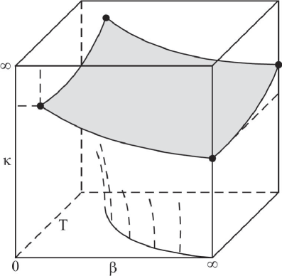
Figure 4: Phase diagram for the $SU(2)$ Higgs model. For a fixed quartic coupling $\lambda=O(1)$ there are three regions in the $\beta,\kappa,T$ parameter space: confinement region for $\beta<\beta_{c},~{}\kappa\ll 1$; Higgs region for $\beta\gg 1,~{}\kappa>\kappa_{c}$; deconfinement region for $\beta>\beta_{c},~{}\kappa<\kappa_{c}$.

For $T=0$ the phase structure is sketched in Fig. 5 in the parameter space $\beta,\kappa,\lambda$. For small values of $\kappa$ the system is in the confinement phase (at $\kappa=0$ the model reduces to a pure $SU(2)$ gauge theory). Along the surface $\Sigma$ there is a first order phase transition to the Higgs phase (with one spin-0 Higgs boson and three massive gauge bosons), except at the boundary $\beta=\infty~{}(g=0)$. The boundary $\partial\Sigma_{1}$ of is a second order transition line as for $T>0$. For small $\beta$ (large coupling) and relatively large values of the hopping parameter $\kappa$ there is an analytic connection between the two regions beyond the boundary piece $\partial\Sigma_{2}$. (This has been established rigorously in [16].) The distinction between confinement and Higgs phases has then no meaning anymore.

If one uses the actual value of the weak coupling constant, it turns out that the finite temperature phase transition always takes place between the Higgs and the deconfinement regions.

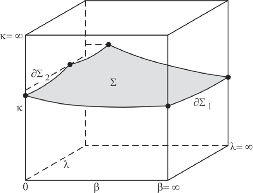
Figure 5: Phase structure for zero temperature (adapted from [7], Sect. 6.1).

One-loop lattice calculation of the effective potential

The effective gauge invariant potential of the $SU(2)$ Higgs model has been determined numerically, along with other quantities [17]. Here, we want to derive the one-loop approximation of this important object. This is an instructive example of lattice perturbation theory.

Let us first consider the ‘broken’ phase. The exponent in (79) has for $V_{x\mu}=1$ a stationary point for the value $\bar{\rho}$ given by

$$\bar{\rho}^{2}=1+\frac{8\kappa+J-1}{2\lambda},$$ (85)

provided $J>1-8\kappa-2\lambda$. In the tree approximation (Laplace approximation of the infinite volume integral) the effective potential is

$$V_{tree}(\Phi^{2})=(1-8\kappa)\Phi^{2}+\lambda(\Phi^{2}-1)^{2}.$$ (86)

(This is convex as a function of $\Phi^{2}$ !) For the one-loop correction we set $\rho_{x}=\bar{\rho}+\sigma_{x},~{}U_{x\mu}=\exp(A_{\mu}(x))$ and consider $A_{\mu}(x)$ as small. The quadratic piece in $\sigma_{x}$ of the exponent in (79) is just the action of a free scalar lattice field $\sigma$ with effective mass

$$m_{\varphi}^{2}=\frac{4}{\kappa}\lambda\bar{\rho}^{2}=m_{H,0}\bar{\rho}^{2}/v^{2},$$ (87)

where $v$ is the value of $|\Phi|$ at the minimum of $V_{tree}(\Phi^{2})$, and $m_{H,0}$ is the zeroth order Higgs mass. According to Sect. 2.2 this gives the following contribution to the one-loop correction

$$V_{1-loop}^{\varphi}(\Phi^{2})=\int_{BZ}\frac{d^{4}k}{(2\pi)^{4}}\frac{1}{2}\ln(\hat{k}^{2}+m_{H}^{2}\Phi^{2}/v^{2}),$$ (88)

where $\hat{k}^{2}:=\sum_{\mu}2(1-\cos k_{\mu})$. For $T>0$ the integral over $k_{4}$ has to be replaced by $T$ times the sum over $k_{4}$, with $k_{4}=(2\pi T)n,~{}n\in\mathbf{Z}$.

For the contribution of the gauge field we set $V_{x\mu}=\exp(A_{\mu}(x))$ and consider $A_{\mu}(x)$ to be small. Then the gauge part of the action reduces in quadratic approximation to the Maxwell action of the three scalar fields $A_{\mu}^{a}$, defined by $A_{\mu}=igA_{\mu}^{a}\tau_{a}/2$. These receive, as in the continuum theory, a mass term from the coupling to the scalar field (last term in (82)) with effective mass

$$m_{g}^{2}=\frac{1}{2}\kappa g^{2}\bar{\rho}^{2}=m_{W,0}^{2}\bar{\rho}^{2}/v^{2},$$ (89)

where $m_{W,0}$ is the zeroth order W-mass.

Next the measure (83) has to be rewritten in the appropriate approximation in terms of $A_{\mu}(x)$ and $\sigma_{x}$. It is a nice exercise in group theory to express the normalized Haar measure $dU$ of $SU(2)$ in terms of the canonical coordinates (of the first kind) $X_{a}$, defined by $U=\exp(iX_{a}\tau_{a}/2)$. The result is

$$dU=\frac{1}{4\pi^{2}}\frac{\sin^{2}(|X|/2)}{|X|^{2}}d^{3}X.$$ (90)

Hence,

$$dV_{x\mu}=\frac{1}{4\pi^{2}}\frac{\sin^{2}(g|A_{\mu}|/2)}{g^{2}|A_{\mu}|^{2}}d^{3}A_{\mu}^{a}~{},$$

with $|A_{\mu}|^{2}=A_{\mu}^{a}A_{\mu}^{a}$. We write the first factor in (83) as

$$\prod_{x,\mu}dV_{x\mu}=e^{-S_{m}}\prod_{x,\mu}dA_{\mu}^{a}~{},$$

with

$$S_{m}=-\sum_{x,\mu}\ln\left(\frac{1}{4\pi^{2}}\frac{\sin^{2}(g|A_{\mu}|/2)}{g^{2}|A_{\mu}|^{2}}\right)=\sum_{x,\mu}\frac{g^{2}}{12}A_{\mu}^{a}A_{\mu}^{a}+O(g^{4}).$$ (91)

(An additive numerical constant was dropped in the last expression.)

In sufficient approximation the measure (83) becomes, up to a normalization,

$$d\mu=\exp\left\{-\sum_{x,\mu,a}\frac{g^{2}}{12}A_{\mu}^{a}A_{\mu}^{a}\right\}\prod_{x,\mu,a}dA_{\mu}^{a}(x)\prod_{x}d\sigma_{x}~{}.$$ (92)

The exponential in this expression is a mass term with mass $g^{2}/6$. This acts like a mass-counter term and diverges in the limit $a\rightarrow 0$. We encounter here an example of a general phenomenon: The lattice regularization provides its own counter terms which ensure renormalizability of the theory.

The contribution of the free massive vector fields $A_{\mu}(x)$ with the effective mass $m_{g}^{2}+g^{2}/6$ gives the following contribution to the one-loop potential (exercise)

$$V_{1-loop}^{g}(\Phi^{2})=9\int_{BZ}\frac{d^{4}k}{(2\pi)^{4}}\frac{1}{2}\ln(\hat{k}^{2}+m_{W}^{2}\Phi^{2}/v^{2}+g^{2}/6).$$ (93)

The reason for the factor 9 is obvious: three massive vector fields with three degrees of freedom. The additive term $g^{2}/6$ in the argument of the logarithm would not appear in a continuum calculation.

We consider now the ‘symmetric’ phase. There is a stationary point at $\bar{\rho}=0$, for which the tree level potential vanishes. The exponent in (79) is now (apart from a sign) the action of a free scalar lattice field $\rho_{x}$ with effective $J$-dependent mass $m_{s}^{2}=m_{0}^{2}-J/\kappa$, plus that of three massless vector fields $A_{\mu}(x)$ which get an effective mass $g^{2}/6$ from the link integration measure in (83). We have to keep in mind that $\rho_{x}$ is a radial variable and that the measure (83) contains the weight factors $\rho_{x}^{3}$. In the steepest decent approximation we obtain for the one-loop free energy density, apart from $J$-independent contributions due to the gauge fields,

$$w(J)\simeq-\int_{BZ}\frac{d^{4}k}{(2\pi)^{4}}\frac{1}{2}\ln(\hat{k}^{2}+2m_{s}^{2}).$$ (94)

The one-loop effective potential is the Legendre transform of $w(J)~{}(\Phi^{2}$ is the conjugate variable). This has to be done numerically.

At the critical temperature the minima of the two effective potentials are degenerate. The critical temperature in units of the Higgs mass as a function of the Higgs mass is shown in the upper part of Fig. 6, both for numerical simulations and perturbation calculations.

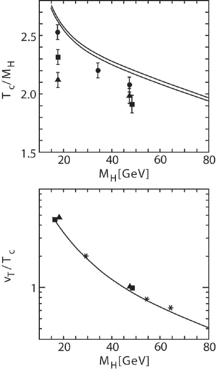
Figure 6: (top panel): Critical temperature as a function of the Higgs mass $m_{H}$. The full squares and triangles are from 4-dimensional simulations with different lattice extensions in the imaginary time direction. The full circles are results from lattice perturbation theory, extrapolated to the continuum. The solid lines are from continuum 2-loop calculations [18]. (From Ref. [19].) (bottom panel): Jump of the order parameter at the critical temperature. The triangles and squares are from the same simulations as in the top panel, and the solid line is again the result of a continuum 2-loop calculation. The starred symbols are from simulations of the so-called 3-dimensional ‘reduced model’ (see footnote 4).

The jump $\Delta$ in the gauge invariant quantity $\rho_{x}^{2},~{}v_{T}:=(\Delta\langle\rho_{x}^{2}\rangle)^{1/2}$, is a measure of the strength of the first order phase transition. Its dependence on the Higgs mass is shown in the lower part of Fig. 6. A similar plot for the latent heat is given in Fig. 7. More recently it has been shown [15] that the first order transition ends at $m_{H}=66.5\pm 1.4~{}GeV$. Above this endpoint only a rapid cross-over can be seen. This number increases for the Standard Model to $72.1\pm 1.4~{}GeV$. In the framework of the effective field theory method (footnote 4) this result has been obtained in [21], [22] and [23] (for a short review, see [24]).

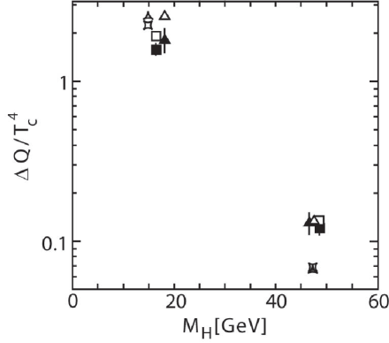
Figure 7: Latent heat as a function of the Higgs mass. The symbols have the same meaning as in the previous figures.

3.2 Baryogenesis and electroweak phase transition

The previous results, in particular Fig.6, are crucial for answering the question whether the cosmological baryon asymmetry might have been generated in the electroweak phase transition. We shall see that this was not the case. Nevertheless, fermion-number violating electroweak interactions are of interest, since they changed the baryon and lepton asymmetries that were generated during earlier epochs, expected in the context of unified extensions of electroweak and strong interactions (GUTs). For reviews, see [25] and [26].

Anomalous fermion number violations

Let me first recall why baryon number (B) and lepton number (L) are not conserved in the Standard Model, although they are obviously conserved in perturbation theory. On the non-perturbative level this due to the chiral nature of the weak interactions. Indeed, this implies that the divergences of the baryon and lepton currents are both anomalous (quantum mechanically non-conserved). It turns out that this violation is such that $B-L$ is conserved.

Consider, for illustration, in the $SU(2)$ Higgs model a massless left-handed fermion doublet $\psi_{L}$ and the global $U(1)$ fermion current

$$J^{\mu}=\bar{\psi}_{L}\gamma^{\mu}\psi_{L}.$$

Classically, this is conserved, and expresses the conservation of the number of fermions corresponding to the field $\psi_{L}$. In quantum theory, the famous triangle anomaly of Adler, Bell and Jackiw leads to the modification

$$\partial_{\mu}J^{\mu}=-\frac{1}{16\pi^{2}}tr(F_{\mu\nu}\tilde{F}^{\mu\nu}),$$ (95)

where $\tilde{F}_{\mu\nu}$ is the dual field strength of the $SU(2)$ gauge field $F_{\mu\nu}$, belonging to the gauge potential $A_{\mu}(x)=-igA_{\mu}^{a}\tau_{a}/2$ (see, e.g., Chap. 19 of [28] or [29] ). The right-hand side of this equation, the famous characteristic second Chern density, has an important topological meaning. Its integral (Chern number) is equal to a certain winding number, as shown below. Locally, it is a divergence of a current. It is more elegant to write this in terms of differential forms. The Chern 4-form belonging to the right-hand side of (95)

$$c_{2}(A)=\frac{1}{8\pi^{2}}tr(F\wedge F)~{}~{}~{}(F=\frac{1}{2}F_{\mu\nu}dx^{\mu}\wedge dx^{\nu})$$ (96)

is (modulo global questions) an exact differential

$$c_{2}=dQ(A),~{}~{}~{}Q(A)=\frac{1}{8\pi^{2}}Tr\Bigl{[}A\wedge(dA+\frac{2}{3}A\wedge A)\Bigr{]}.$$ (97)

$Q(A)$ is the Chern-Simons form ($A=A_{\mu}dx^{\mu}$). This 3-form is not gauge invariant. If we integrate (95), i.e.,

$$d\star J=c_{2}(A)$$ (98)

over a region $\mathcal{D}$ of space-time between two time slices, Stokes’ theorem gives

$$\int_{\mathcal{D}}d\star J=\int_{t=t_{2}}\star J-\int_{t=t_{1}}\star J=\Delta N_{CS},$$

where $N_{CS}$ is the difference of the Chern-Simons numbers

$$\Delta N_{CS}[A]=\int_{t=t_{2}}Q(A)-\int_{t=t_{1}}Q(A).$$ (99)

This difference is gauge invariant since it is equal to the integral of $c_{2}(A)$ over $\mathcal{D}$. We see that the change of the fermion number $\Delta N_{F}$ associated to $\psi_{L}$ is equal to $\Delta N_{CS}$:

$$\Delta N_{F}=\Delta N_{CS}[A].$$ (100)

Before further elaborating on this, we consider the left-handed doublets of the three families of leptons and quarks of the Standard Model. The previous equation implies the same fermion-number change for each species. For the leptons the changes of lepton number are

$$\Delta N_{e}=\Delta N_{\mu}=\Delta N_{\tau}=\Delta N_{CS}[A],$$ (101)

and the changes for the quarks imply the following change of the baryon number

$$\Delta B=\frac{1}{3}\cdot 3\cdot 3~{}\Delta N_{CS}[A]$$ (102)

($\frac{1}{3}$ from the baryon number of quarks, $3\cdot 3$ from the three colors and number of generations). This also shows that $B-L$ is conserved.

The non-perturbative effects we are discussing involve strong gauge fields, and it is therefore reasonable to treat them classically. So let us now consider classical field configurations and the changes of their Chern-Simons numbers in time. In particular, we are interested in field configurations which interpolate between different classical vacua with pure gauges $A_{\mu}=U^{-1}\partial_{\mu}U,~{}U(x)$ an $SU(2)$-valued function. The Chern-Simons number of such a vacuum gauge field is in general different from zero. A short calculation gives

$$Q(A)=-\frac{1}{24\pi^{2}}Tr\Bigl{(}U^{-1}dU\wedge U^{-1}dU\wedge U^{-1}dU\Bigr{)}.$$ (103)

We assume that for fixed time $U(x)$ converges at infinity to $1_{2}$ in such a manner that we can regard it as a function on the compactified space $S^{3}$. Since $SU(2)$ is topologically also a three-sphere, we then have a map from $S^{3}$ to $S^{3}$. We now show that the winding number (degree) of this map is just the Chern-Simons number of the pure gauge. The easiest way to see this is to note first that $U^{-1}dU$ is the pull-back by $U$ of the Maurer-Cartan form $\theta$ on $SU(2)$:

$$U^{-1}dU=U^{\star}(\theta).$$

Therefore, Eq.(103) can be written as

$$Q(U^{-1}dU)=-\frac{1}{24\pi^{2}}U^{\star}\Bigl{[}Tr(\theta\wedge\theta\wedge\theta)\Bigr{]}.$$ (104)

A general result on winding numbers tells us that the one for $U:~{}S^{3}\rightarrow S^{3}$ is

$$n(U)=\frac{\int_{S^{3}}U^{\star}(\omega)}{\int_{SU(2)}(\omega)}$$

for any volume form $\omega$ on $S^{3}$ (see, e.g., Sect. 7.5 of [31]), in particular for $\omega=Tr(\theta\wedge\theta\wedge\theta)$. Hence,

$$N_{CS}[U^{-1}dU]=n(U)(-\frac{1}{24\pi^{2}})\int_{SU(2)}\omega.$$

But $(-1/24\pi^{2})\omega$ is the three-form corresponding to the normalized Haar measure, whence

$$N_{CS}[U^{-1}dU]=n(U).$$ (105)

This integer characterizes topologically different vacua.

As a result of these considerations we obtain for a field configuration which interpolates between vacua at $t=-\infty$ and $t=+\infty$

$$\Delta N_{CS}[U^{-1}dU]=\left.n(U)\right|_{t=\infty}-\left.n(U)\right|_{t=-\infty}.$$ (106)

This difference is also equal to the second Chern number

$$c_{2}=\int c_{2}(A),$$

which is, of course, gauge invariant.

The winding number $n(U)$ also shows up in the vacuum configuration of the Higgs field. It is straightforward to verify the following identity (we omit the wedge symbols):

$$Tr[(\phi^{\dagger}d\phi)^{3}]-3Tr[A(dA+\frac{2}{3}A^{2})]=Tr[(\phi^{\dagger}D\phi)^{3}]-3Tr(\phi\dagger FD\phi)+3d(A~{}d\phi~{}\phi^{\dagger}).$$ (107)

This implies that the left-hand side is gauge invariant, up to an exact differential. Apart from this exact differential the right-hand side vanishes for a classical vacuum, where $D\phi=0$. Integrating the last equation we see that the winding number of the Higgs vacuum field

$$N_{H}=\frac{1}{24\pi^{2}}\int Tr[(\phi^{\dagger}d\phi)^{3}]$$ (108)

is equal to the Chern-Simons number, and for a vacuum-vacuum transition we obtain the gauge invariant relation

$$\Delta N_{CS}=\Delta N_{H}.$$ (109)

For the smallest non-vanishing change (102) gives

$$\Delta B=-\Delta L=3,$$ (110)

the quantum numbers of 12 left-handed fermions. States such as $\prod u_{L}d_{L}d_{L}\nu_{L}$, where $\Pi$ denotes the product over all generations, can be created out of the vacuum. (Altogether there are 12 such combinations.)

Vacua with different topological numbers $n$ are separated by a potential barrier, because a transition has to involve non-vacuum fields. At zero temperature and ‘low’ energies such a transition is a tunnelling process that can be estimated by using (constraint) instantons. For a pure Yang-Mills theory an instanton minimizes the Euclidean action in the sector with Chern number $c_{2}=1$. For $SU(2)$ the corresponding action is equal to $8\pi^{2}/g^{2}$, hence the tunnelling probability is enormously suppressed by the factor $\exp(-4\pi/\alpha_{W})\sim 10^{-170}$, where $\alpha_{W}=g^{2}/4\pi=\alpha/\sin^{2}\theta_{W}\simeq 1/29~{}(\theta_{W}$ is the weak mixing angle). When the system is in the Higgs phase things are somewhat more complicated, since there is then no minimum for the Euclidean action with $c_{2}=1$. Nevertheless, the tunnelling rate is suppressed by the same exponential factor. (For details, see [32].)

Things are very different at high temperatures, corresponding to energy scales set by the height of the barrier. This is given by the static saddle point solution of the bosonic sector (Yang-Mills-Higgs equations), the so-called sphaleron solution. The energy of this spherically symmetric unstable solution is [33]

$$E_{sph}=\frac{2m_{W}}{\alpha_{W}}f(\frac{m_{H}}{m_{W}}),$$ (111)

where the function varies from 1.56 to 2.72 as $m_{H}/m_{W}$ varies from zero to large values. The height of the barrier is thus of order 10 TeV. At temperatures larger than the critical temperature $T_{c}\sim m_{H}/g,B$-violating processes may proceed through thermal activation over the barrier which is then much lower because the $W$ boson mass eventually vanishes. The tunnelling suppression factor $\exp(-E_{sph}/T)$ is no more effective in the symmetric phase. Detailed studies [34] have established that the naive power counting estimate for the rate per unit volume in the unbroken phase

$$\Gamma=\mathcal{O}(1)(\alpha_{W}T)^{4}$$ (112)

indeed holds. (For a review, see [27].) We compare this with the expansion rate $H$ of the Universe. During these early phases the energy density $\rho$ is dominated by relativistic particles, thus $\rho=g_{\ast}(\pi^{2}/30)T^{4}$, where $g_{\ast}$ is the effective number of degrees of freedom per particle (2 for the photon). The Friedmann equation gives

$$H\simeq g_{\ast}^{1/2}T^{2}/M_{Planck}$$

with $g_{\ast}^{1/2}=\mathcal{O}(10)$. For dimensional reasons, $\Gamma$ should be compared with the time derivative of $T^{3}$ ( a typical particle density), i.e. with $HT^{3}$. (We used that $T$ is most of the time inversely proportional to the expansion factor.) The ratio

$$\frac{\Gamma}{HT^{3}}\sim\alpha_{W}^{4}\frac{M_{Planck}}{T}$$

is much larger than 1 for $T_{c}<T<10^{12}~{}GeV$. In the symmetric phase the $B$-violating reactions are thus fast enough to maintain thermal equilibrium.

During this phase the $B+L$ part of $B=\frac{1}{2}(B-L)+\frac{1}{2}(B+L)$ is therefore changed. At first sight one might expect that it is completely washed out, and that $B=-L=\frac{1}{2}(B-L)_{initial}$ is established. Things are, however, somewhat more complicated, since only the fermion currents of the left-handed doublets have an anomaly. Moreover, electrical charge neutrality has to be taken into account. A more careful analysis shows [35], [36] that in good approximation one ends up above $T_{c}$ with

$$B+L=-\frac{23}{79}(B-L)$$ (113)

for the Standard Model with three generations and one Higgs doublet. (A mass correction [36] changes this slightly.) Without a primordial $B-L$ (e.g. from GUT physics) both $B$ and $L$ would vanish. These considerations are relevant for scenarios of leptogenesis (see [26]).

Evolution below $T_{c}$

The electroweak phase transition cannot generate the cosmological baryon asymmetry, because the last of the following Sakharov conditions is not fulfilled:

$\bullet$ Violation of baryon number

$\bullet$ Violation of $C$ and $CP$

$\bullet$ Deviations from thermodynamic equilibrium.

The first two of these are obviously necessary. (The possibility that the Universe is symmetric on scales much larger than the present horizon, but not in our visible part, will be briefly discussed in the next section) The third condition requires some explanation. A simple manner to understand its necessity is this: In thermodynamic equilibrium one looses in a way the arrow of time (on cosmological short time scales), hence the guaranteed $CTP$ symmetry implies $CP$ conservation. A more formal argument goes as follows: In equilibrium the density matrix that maximizes the entropy for given average values of the absolutely conserved ‘charges’ $Q_{i}$ is the grand canonical ensemble

$$\varrho=Z^{-1}\exp\Bigl{[}-\beta(H-\sum_{i}\mu_{i}Q_{i})\Bigr{]}$$

($\mu_{i}=$chemical potentials for the conserved charges $Q_{i}$). Suppose that $B$ and $L$ are independently violated, and that beside the electric charge $Q$ no other charges like $B-L$ are conserved. Because of electrical charge neutrality $\varrho$ the has to be the canonical ensemble: $\varrho=Z^{-1}e^{-\beta H}$. But $H$ is invariant under the $CPT$ operation $\theta$. Since $B$ is odd under $\theta$, we have

$$\langle B\rangle=Z^{-1}Tr(Be^{-\beta H})=Z^{-1}Tr\Bigl{[}\theta(Be^{-\beta H})\theta^{-1}\Bigr{]}=-\langle B\rangle.$$

So in thermodynamic equilibrium any previous baryonic and leptonic asymmetries would be washed out. Note that such an argument could not be used above, since not only $B-L$, but also all the anomaly free fermionic charges $N_{i}-\frac{1}{3}B,~{}i=e,\mu,\tau$ (see (101) and (102)) are conserved. For this reason there remain, after imposing charge neutrality, three independent chemical potentials. That $B+L$ in (113) depends only on $B-L$ is the result of the approximations used in [35], [36]. Similarly, baryonic and leptonic asymmetries may not be completely washed out if, beside the electric charge, there would exist other absolutely conserved charges whose chemical potentials are non-vanishing. Below $T_{c}$, as long as the ‘sphaleron processes’ are sufficiently fast to establish thermal equilibrium, the combination $B+L$ is no more proportional to $B-L$. As a result, even if $B-L$ should vanish for all temperatures, a non-vanishing $B$ would result (mass effects are important for this).

In a strongly first order transition there would be a departure from thermal equilibrium and anomalous $B$ and $L$ violating processes could produce an asymmetry (with $B-L=0$). Indeed, the transition would be very violent through nucleation of bubbles in the new phase which would expand and collide. In order that the asymmetry is not erased after the phase transition, the sphaleron energy at $T_{c}$ must be sufficiently high. This leads to the following condition for the jump $v_{T}$ of the order parameter plotted in Fig. 7:

$$v_{T}/T_{c}>1.$$ (114)

For a detailed discussion and references we refer to Sect. 7 of [27]. The results shown in Fig. 6 already imply that the electroweak transition in the Standard Model is too weak for baryogenesis. As discussed earlier, the transition even stops to be of first order for Higgs masses higher than $\simeq 72~{}GeV$, much below the LEP limit $m_{H}>110~{}GeV$.

In summary, the baryon asymmetry of the Universe must have been produced at energies much higher than the electroweak scale. Part of the $B+L$ component will later be washed out by anomalous weak processes, but the $B-L$ component would be preserved. Electroweak baryosynthesis is only possible in extensions of the Standard Model. The matter-antimatter asymmetry of the Universe is strong evidence for physics beyond the Standard Model. Possible scenarios have been reviewed many times; see, e.g., [37], [26].

3.3 QCD phase transition

At temperatures of the order of the pion mass the pions are so abundant that they begin to overlap. As a result, the interactions of their constituents (quarks and gluons) become important.

For a rough estimate, consider the number density of a free pion gas in the early Universe at $T\ll m_{N}$ (nucleon mass). We can take their chemical potential equal to zero, because the pions are much more abundant than the nucleons. Their number density is for $T>m_{\pi}$:

$$n_{\pi}(T)=3\int\frac{1}{e^{\varepsilon(p)/T}-1}\frac{d^{3}p}{(2\pi)^{3}}\simeq\frac{3\zeta(3)}{\pi^{2}}T^{3}.$$

The volume $v_{\pi}$ of a pion is $(4\pi/3)r_{\pi}^{3}$, with the pion radius $r_{\pi}\simeq 0.6~{}fm$. We find $n_{\pi}(T)v_{\pi}=1$ at a temperature $T\simeq 285~{}MeV$, with an energy density of $\simeq 850~{}MeV/fm^{3}$.

On the basis of the asymptotic freedom of QCD one naturally expects that at high temperatures the hadronic matter behaves as an asymptotically free gas of quarks and gluons (quark-gluon plasma). Somewhere in the region $T\sim m_{\pi}$ there should be a phase transition or crossover between the low energy hadronic matter – with confinement and broken chiral symmetry – and the quark-gluon plasma. The study of the existence and nature of this phase transition is a central theme of QCD. One is, of course, also interested in the equation of state.

Because of serious infrared singularities, perturbation theory is of limited value, even for the treatment of the asymptotic behavior of the quark-gluon plasma. This is even more so when the phase transition is addressed. Therefore, the non-perturbative lattice approach is the only way to investigate the thermodynamics of hadrons from first principles. A lot of work has been invested in this domain over many years. Very useful general references are [7], [38] and [39]. Since the critical temperature is close to the strange quark mass, it is important to simulate dynamical light quark flavors realistically. This has almost been achieved by now. A recent study of the MILC collaboration [40] comes to the conclusion that in the real world there is presumably no bona fide phase transition at the physical quark masses. In Fig. 8 we reproduce the result for the order parameter $\langle\bar{\psi}\psi\rangle$ for two degenerate light quarks (up and down) plus the strange quark with its physical mass.

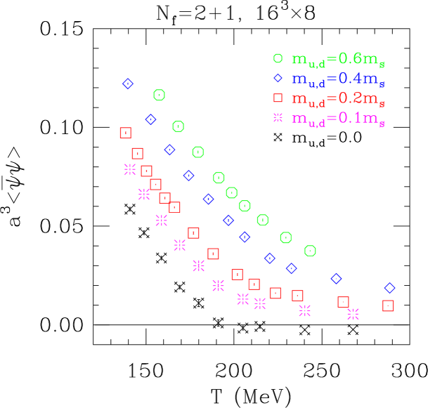
Figure 8: The chiral order parameter, $\bar{\psi}\psi$, on $16^{3}\times 8$ lattices (from Ref. [40]).

Fig. 9 shows the real part of the Wilson line or Polyakov loop, defined as (using the notation $U_{\mu}(x)$ for the link variables)

$$L(\mathbf{x})=Tr\left\{\prod_{x_{4}=1}^{N_{t}}U_{4}(\mathbf{x},x_{4})\right\},$$ (115)

with $N_{t}=\beta/a$. This quantity is gauge invariant. The logarithm of its expectation value is proportional to the free energy of the system with a single heavy quark, measured relative to that in the absence of such a quark. $\langle L\rangle=0$ can be interpreted as signalizing confinement.

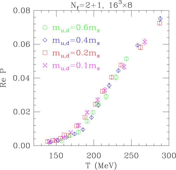
Figure 9: The real part of the Polyakov loop on $16^{3}\times 8$ lattices (from Ref. [40]).

These and other results suggest that there is a crossover, rather than a sharp phase transition from the confined to the unconfined behavior. Similar results were obtained in [41].

Many cosmological speculations connected with the QCD transition (possibility of inhomogeneous nucleosynthesis, strange quark nuggets, etc) have been discussed. Since it is not clear whether there are any observable footprints of this transition the Universe passed through (and for limitations of time), I leave this interesting subject.

In the central regions of neutron stars matter is squeezed to densities several times higher than the nuclear density, $\rho_{nuc}=2.8\times 10^{14}~{}g~{}cm^{-3}$ (see, e.g., Chap.6 of [42]). One expects that these regions are, at least for the most massive neutron stars, in the deconfined chirally symmetric phase. It is also expected that at relatively low temperatures the transition to this state of matter as a function of baryon chemical potential $\mu_{B}~{}(=3\mu_{quark})$ is first order for realistic quark masses. It is difficult to perform lattice simulations for $\mu_{B}\neq 0$, because the quark determinant (arising from the functional integral over the quark fields) becomes complex, and thus also the corresponding term in the effective action. For a clear discussion of these difficulties we refer to Sect.5.4.3 of [7]. Recently, significant progress has been made in algorithms, and realistic calculations may become feasible.

3.4 Cosmic topological defects

The formation of topological defects is well-known to condensed matter physicists. A classic example is the formation of vortices in type II superconductors. As you all know these are described by the Ginzburg-Landau theory, which is a ‘spontaneously broken’ gauge theory (the Abelian Higgs model). The complex order parameter $\phi(x)$, which later turned out to be proportional to the gap function in BCS theory, plays in particle physics language the role of a Higgs field. I recall that the integer number in the flux quantization is also the degree (winding number) of the map which associates to each direction in the two-dimensional transverse space (topologically a circle $S^{1}$) the asymptotic value of $\phi$ in the vacuum manifold. The latter is the circle on which $|\phi|$ assumes the minimum of the Ginzburg-Landau (Higgs) potential.

The analogous ’t Hooft-Polyakov monopoles exist, for example as solutions of the $SU(2)$-Higgs model. The pole strength is then again topologically quantized, and the corresponding integer number is this time the winding number of the map which associates to each direction of 3-space (topologically $S^{2}$) the asymptotic value of $\phi$ in the vacuum manifold, that is this time an $S^{2}$. Note that the gauge group $SU(2)$acts on this vacuum manifold transitively and is thus topologically isomorphic to the homogeneous space $SU(2)/H$, where $H=U(1)$ is the stabilizer of any point of the vacuum manifold. For a general gauge theory with gauge group $G$, non-Abelian (regular) monopoles exist if the second homotopy group of $G/H~{}(H$ is again the stabilizer of the vacuum manifold) is non-trivial. Homotopy theory allows to compute these homotopy groups quite easily.

Textures are also known in condensed matter physics. These are classified by a third homotopy group.

The theory of topological defects in cosmology is extensively described in the monograph [43]. On the basis of what we now know about the cosmic microwave background, the conclusion is inevitable that topological defects played no important role in large scale structure formation. This is the main reason why interest in the subject has declined.

4 Vacuum energy problem and Dark Energy

In the course of the various ‘phase’ transitions the Universe passed through, the free energy density changed by a huge amount in comparison to the present day cosmological energy density (which is close to the critical value). This gives me the opportunity to discuss the cosmological constant problem, a profound mystery indeed of present day physics.

4.1 Vacuum energy and gravity

When we consider the coupling to gravity, the vacuum energy density acts like a cosmological constant. In order to see this, first consider the vacuum expectation value of the energy-momentum tensor in Minkowski spacetime. Since the vacuum state is Lorentz invariant, this expectation value is an invariant symmetric tensor, hence proportional to the metric tensor. For a curved metric this is still the case, up to higher curvature terms:

$$<T_{\mu\nu}>_{vac}=g_{\mu\nu}\rho_{vac}+\textit{higher curvature terms}.$$ (116)

The effective cosmological constant, which controls the large scale behavior of the Universe, is given by

$$\Lambda=8\pi G\rho_{vac}+\Lambda_{0},$$ (117)

where $\Lambda_{0}$ is a bare cosmological constant in Einstein’s field equations.

We know from astronomical observations since a long time that $\rho_{\Lambda}\equiv\Lambda/8\pi G$ can not be larger than about the critical density:

$$\rho_{crit} = \frac{3H_{0}^{2}}{8\pi G}$$

$$= 1.88\times 10^{-29}h_{0}^{2}~{}\textit{g}~{}\textit{cm}^{-3}$$

$$\simeq (3\times 10^{-3}eV)^{4},$$

where $h_{0}$ is the reduced Hubble parameter

$$h_{0}=H_{0}/(100~{}\textit{km}~{}\textit{s}^{-1}\textit{Mpc}^{-1})$$ (119)

and is close to 0.7.

It is a complete mystery as to why the two terms in (117) should almost exactly cancel. This is – more precisely stated – the famous $\Lambda$-problem.

As far as I know, apart some unpublished remarks of Pauli in the early 1920’s [44], the first who wondered about possible contributions of the vacuum energy density to the cosmological constant was Zel’dovich . He discussed this issue in two papers [45] during the third renaissance period of the $\Lambda$-term, but before the advent of spontaneously broken gauge theories. The following remark by him is particularly interesting. Even if one assumes completely ad hoc that the zero-point contributions to the vacuum energy density are exactly cancelled by a bare term, there still remain higher-order effects. In particular, gravitational interactions between the particles in the vacuum fluctuations are expected on dimensional grounds to lead to a gravitational self-energy density of order $G\mu^{6}$, where $\mu$ is some cut-off scale. Even for $\mu$ as low as 1 GeV (for no good reason) this is about 9 orders of magnitude larger than the observational bound.

This illustrates that there is something profound that we do not understand at all, certainly not in quantum field theory ( so far also not in string theory). We are unable to calculate the vacuum energy density in quantum field theories, like the Standard Model of particle physics. But we can attempt to make what appear to be reasonable order-of-magnitude estimates for the various contributions. All expectations (some of which are discussed below) are in gigantic conflict with the facts. Trying to arrange the cosmological constant to be zero is unnatural in a technical sense. It is like enforcing a particle to be massless, by fine-tuning the parameters of the theory when there is no symmetry principle which implies a vanishing mass. The vacuum energy density is unprotected from large quantum corrections. This problem is particularly severe in field theories with spontaneous symmetry breaking. In such models there are usually several possible vacuum states with different energy densities. Furthermore, the energy density is determined by what is called the effective potential, and this is dynamically determined. Nobody can see any reason why the vacuum of the Standard Model we ended up as the Universe cooled, has – for particle physics standards – an almost vanishing energy density. Most probably, we will only have a satisfactory answer once we shall have a theory which successfully combines the concepts and laws of general relativity about gravity and spacetime structure with those of quantum theory.

4.2 Simple estimates of vacuum energy contributions

If we take into account the contributions to the vacuum energy from vacuum fluctuations in the fields of the Standard Model up to the currently explored energy, i.e., about the electroweak scale $M_{F}=G_{F}^{-1/2}\approx 300~{}GeV~{}(G_{F}:$ Fermi coupling constant), we cannot expect an almost complete cancellation, because there is no symmetry principle in this energy range that could require this. The only symmetry principle which would imply this is supersymmetry, but supersymmetry is broken (if it is realized in nature). Hence we can at best expect a very imperfect cancellation below the electroweak scale, leaving a contribution of the order of $M_{F}^{4}$ . (The contributions at higher energies may largely cancel if supersymmetry holds in the real world.)

We would reasonably expect that the vacuum energy density is at least as large as the condensation energy density of the QCD transition to the confined phase of broken chiral symmetry. Already this is far too large, namely of the order $\sim\Lambda_{QCD}^{4}/16\pi^{2}\sim 10^{-4}\textit{GeV}^{4}$, i.e., more than 40 orders of magnitude larger than $\rho_{crit}$. Beside the formation of quark condensates $<\bar{q}q>$ in the QCD vacuum which break chirality, one also expects a gluon condensate $<G^{\mu\nu}_{a}G_{a\mu\nu}>\sim\Lambda_{QCD}^{4}.$ This produces a significant vacuum energy density as a result of a dilatation anomaly: If $\Theta_{\mu}^{\mu}$ denotes the “classical” trace of the energy-momentum tensor, we have [46]

$$T^{\mu}_{\mu}=\Theta^{\mu}_{\mu}+\frac{\beta(g_{3})}{2g_{3}}G^{\mu\nu}_{a}G_{a\mu\nu},$$ (120)

where the second term is the QCD piece of the trace anomaly ($\beta(g_{3})$ is the $\beta$-function of QCD that determines the running of the strong coupling constant). I recall that this arises because a scale transformation is no more a symmetry if quantum corrections are included. Taking the vacuum expectation value of (120), we would again naively expect that $<\Theta_{\mu}^{\mu}>$ is of the order $M_{F}^{4}$. Even if this should vanish for some unknown reason, the anomalous piece is cosmologically gigantic. The expectation value $<G^{\mu\nu}_{a}G_{a\mu\nu}>$ can be estimated with QCD sum rules [47], and gives

$$<T^{\mu}_{\mu}>^{anom}\sim(350MeV)^{4},$$ (121)

about 45 orders of magnitude larger than $\rho_{crit}$. The expected energy density is larger than the energy-mass density in a neutron star. This reasoning should show convincingly that the cosmological constant problem is indeed a profound one. (Note that there is some analogy with the (much milder) strong CP problem of QCD. However, in contrast to the $\Lambda$-problem, Peccei and Quinn [48] have shown that in this case there is a way to resolve the conundrum.)

Let us also have a look at the Higgs condensate of the electroweak theory. Recall that in the Standard Model we have for the Higgs doublet $\Phi$ in the broken phase for $<\Phi^{*}\Phi>\equiv\frac{1}{2}\phi^{2}$ the potential

$$V(\phi)=-\frac{1}{2}m^{2}\phi^{2}+\frac{\lambda}{8}\phi^{4}.$$ (122)

Setting as usual $\phi=v+H$, where $v$ is the value of $\phi$ where $V$ has its minimum,

$$v=\sqrt{\frac{2m^{2}}{\lambda}}=2^{-1/4}G_{F}^{-1/2}\sim 246GeV,$$ (123)

we find that the Higgs mass is related to $\lambda$ by $\lambda=M_{H}^{2}/v^{2}$. For $\phi=v$ we obtain the energy density of the Higgs condensate

$$V(\phi=v)=-\frac{m^{4}}{2\lambda}=-\frac{1}{8\sqrt{2}}M_{F}^{2}M_{H}^{2}=\mathcal{O}(M_{F}^{4}).$$ (124)

We can, of course, add a constant $V_{0}$ to the potential (122) such that it cancels the Higgs vacuum energy in the broken phase – including higher order corrections. This again requires an extreme fine tuning. A remainder of only $\mathcal{O}(m_{e}^{4})$, say, would be catastrophic. This remark is also highly relevant for models of inflation and quintessence.

In attempts beyond the Standard Model the vacuum energy problem so far remains, and often becomes even worse. For instance, in supergravity theories with spontaneously broken supersymmetry there is the following simple relation between the gravitino mass $m_{g}$ and the vacuum energy density

$$\rho_{vac}=\frac{3}{8\pi G}m_{g}^{2}.$$

Comparing this with eq.(30) we find

$$\frac{\rho_{vac}}{\rho_{crit}}\simeq 10^{122}\Bigl{(}\frac{m_{g}}{m_{Pl}}\Bigr{)}^{2}.$$

Even for $m_{g}\sim 1\;eV$ this ratio becomes $10^{66}$. ($m_{g}$ is related to the parameter $F$ characterizing the strength of the supersymmetry breaking by $m_{g}=(4\pi G/3)^{1/2}F$, so $m_{g}\sim 1\;eV$ corresponds to $F^{1/2}\sim 100\;TeV$.)

Also string theory has not yet offered convincing clues why the cosmological constant is so extremely small. The main reason is that a low energy mechanism is required, and since supersymmetry is broken, one again expects a magnitude of order $M_{F}^{4}$, which is at least 50 orders of magnitude too large (see also [49]). However, non-supersymmetric physics in string theory is at the very beginning and workers in the field hope that further progress might eventually lead to an understanding of the cosmological constant problem.

I hope I have convinced you, that there is something profound that we do not understand at all, certainly not in quantum field theory, but so far also not in string theory.

For more on this, see e.g. [44] (and references therein).

4.3 Astronomical evidence for Dark Energy

A wide range of astronomical data support the following ‘concordance’ $\Lambda$- Cold- Dark- Matter ($\Lambda$CDM) model: The Universe is spatially flat and dominated by vacuum energy density or an effective equivalent, and weakly interacting cold dark matter. Furthermore, the primordial fluctuations are adiabatic and nearly scale invariant, as predicted in simple inflationary models. It is very likely that the present concordance model will survive. The evidence for a dark energy component of about 0.7 times the critical energy density is steadily increasing, and by the time the proceedings of this school will be available one can presumably make stronger statements. Readable reviews (for people outside the field) of the current evidence for a nearly homogeneous energy density with negative pressure that dominates the energy content of the recent and future Universe are [50], [51]. Beside, there is a rapidly growing semi-popular literature on this exciting subject, confronting us with really profound fundamental physics questions.

References

- [1] M. Le Bellac, Thermal Field Theory, Cambridge Univ. Press, (1996).
- [2] J. Kapusta, Finite-Temperature Field Theory, Cambridge Monographs on Mathematical Physics, Cambridge University Press, 1989.
- [3] M. Aizenman, Phys. Rev. Lett. 47, 1 (1981); J. Fröhlich, Nucl. Phys. B200, 281 (1982).
- [4] J. Zinn-Justin, Quantum Field Theory and Critical Phenomena, Fourth Edition, Clarendon Press, Oxford, 2002.
- [5] K. Cahill, Phys. Rev. D52, 4704 (1995).
- [6] S. Elitzur, Phys. Rev. D12, 3978, (1975).
- [7] I. Montvay and G. Münster, Quantum Fields on a Lattice, Cambridge University Press, 1994.
- [8] H.J. Rothe, Lattice Gauge Theories: An Introduction, World Scientific, 1997.
- [9] S. Chandrasekharan and U.-J. Wiese, hep-lat/0405024.
- [10] L. O’Raifeartaigh, A. Wipf and H. Yoneyama, Nucl. Phys. B271, 635 (1986).
- [11] K. Holland and J. Kuti, Nucl. Phys. B (Proc. Supp.) 129-130, 765 (2004).
- [12] R.T. Rockafellar, Convex Analysis,Princeton Univ. Press, Princeton, 1970.
- [13] R.S. Ellis, Entropy, Large Deviations, and Statistical Mechanics, Springer-Verlag, 1985.
- [14] B. Simon, The Statistical Mechanics of Lattice Gases, Vol. 1, Princeton Univ. Press, 1993.
- [15] Z. Fodor, Nucl. Phys. B (Proc. Supp.) 83-84, 121 (2000); hep-lat/9909162.
- [16] K. Osterwalder and E. Seiler, Ann. Phys. 110, 440, (1978).
- [17] Z. Fodor, J. Hein, K. Jansen, A. Jaster, I. Montvay, B439, 147 (1995); hep-lat/9409017.
- [18] W. Buchmüller, Z. Fodor, A. Hebecker, Nucl. Phys. B447, 317 (1995).
- [19] K. Jansen,Nucl. Phys. B (Proc. Supp.) 47, 196 (1996); hep-lat/9509018.
- [20] M.E. Shaposhnikov, Proc. Int. School of Subnuclear Phys. (Erice 1996), World Scientific, hep-ph/9610247.
- [21] K. Kajantie, M. Laine, K. Rummukainen and M.E. Shaposhnikov, Phys. Rev. Lett. 77, 2887 (1996); hep-ph/9605288.
- [22] K. Rummukainen, M. Taypin, K. Kajantie, M. Laine and M.E. Shaposhnikov, Nucl. Phys. B532, 283 (1998); hep-lat/9805013.
- [23] M. Laine and K. Rummukainen, Nucl. Phys. Proc. Suppl. 73, 180 (1999); hep-lat/9809045.
- [24] M. Laine, hep-ph/0111349.
- [25] A.G. Cohen, D.B. Kaplan and A.E. Nelson, Annu. Rev. Nucl. Part Sci. 43, 27 (1993).
- [26] M. Dine and A. Kusenko, Origin of the matter-antimatter asymmetry, Rev. Mod. Phys. 76, 1 (2004).
- [27] V.A. Rubakov and M.E. Shaposhnikov, Usp. Fis. Nauk. 166, 493 (1996); hep-ph/9603208.
- [28] M.E. Peskin and D.V. Schroeder, An Introduction to Quantum Field Theory, Addison-Wesley (1995).
- [29] M. Nakahara, Geometry, Topology and Physics, Adam Hilger, Bristol and New York, 1990.
- [30] M. Lüscher, Phys. Lett. B428, 342 (1998).
- [31] R. Abraham, J. Marsden, and T. Ratiu, Manifolds, Tensor Analysis, and Applications, Addison-Wesley, 1983.
- [32] I. Affleck, Nucl. Phys. B191, 455 (1981).
- [33] F.R. Klinkhamer and N.S. Manton, Phys. Rev. D30, 2212 (1984).
- [34] P. Arnold, D. Son, and L.G. Yaffe, Phys. Rev. D 55, 6264 (1997); Phys. Rev. D 62, 023512 (2000).
- [35] J.A. Harvey and M.S. Turner, Phys. Rev. D42, 3344 (1990).
- [36] H. Dreiner and G.G. Ross, Nucl. Phys. B410, 188 (1993).
- [37] A. Riotto and M. Trodden, Ann. Rev. Nucl. Part. Sci. 49, 35 (1999).
- [38] F. Karsch, Lect. Notes Phys. 583, 209 (2002).
- [39] S. Gottlieb, J. Phys. G30, S421 (2004).
- [40] C. Bernard, et al., hep-lat/0405029.
- [41] F. Karsch, et al., hep-lat/0309116.
- [42] N. Straumann, General Relativity, With Applications to Astrophysics, Texts and Monographs in Physics, Springer Verlag, 2004.
- [43] A. Vilenkin and E.P.S. Shellard, Cosmic Strings and other Topological Defects, Cambridge University Press, 1994.
- [44] N. Straumann, in Séminaire Poincaré 2002. Vacuum Energy – Renormalization, Birkhäuser-Verlag 2003; astro-ph/0203330.
- [45] Y.B. Zel’dovich, JETP letters 6, 316 (1967); Soviet Physics Uspekhi 11, 381 (1968).
- [46] C.G. Callan, S. Coleman, and R. Jackiw, Ann.Phys.59, 42 (1970).
- [47] T. Schäfer and E.V. Shuryak, Rev. Mod. Phys. 70, 323 (1998).
- [48] R.D. Peccei and H. Quinn, Phys. Rev. Lett, 38, 1440 (1977); Phys. Rev. D16, 1791 (1977).
- [49] E. Witten, hep-ph/0002297.
- [50] W. Hu and S. Dodelson, Annu. Rev. Astron. Astrophys. 40, 171-216 (2002).
- [51] S. Dodelson, Modern Cosmology, Academic Press, 2003.