Strong Gravitational Lenses in a Cold Dark Matter Universe
A dissertation submitted to the University of Tokyo
in partial fulfillment of the requirements
for the degree of Doctor of Science in Physics
Masamune Oguri
Department of Physics, University of Tokyo
April, 2004

Abstract

We present theoretical and observational studies of strong gravitational lenses produced by clusters of galaxies. Our purpose is to test the Cold Dark Matter (CDM) model at small and highly non-linear scales where it has been claimed that the CDM model may confront several difficulties. We concentrate our attention on the statistics of strong gravitational lenses because the strong lensing is sensitive to the mass distributions of central, high-density regions of lensing clusters where the cold and collisionless hypotheses on dark matter are crucial. We use two complementary statistics, lensed arcs and quasars, to probe the mass distributions.

First, we construct a triaxial lens model, and develop a new method to include triaxiality of dark halos in the lens statistics. We find that the effect of triaxiality is significant; it enhances lensing probabilities by a factors of a few to ten, assuming the degree of triaxiality predicted in the CDM model. Thus it is essential to take triaxiality into account in the lens statistics. In particular, we argue that both central concentration and large triaxiality of dark halos are required to reproduce the observed number of arcs in clusters; thus the result can be interpreted as a strong evidence for the cold and collisionless dark matter.

One of the most notable advantages of the triaxial modeling over the spherical modeling is that the triaxial modeling allows us to predict image multiplicities. We find that the CDM halos predict significant fraction (more than 20%) of naked cusp lenses, unlike lensing by isothermal galaxies where naked cusp configurations are rare. In addition, we point out the image multiplicities depend strongly on the central concentration of dark halos. Therefore we propose image multiplicities as a new powerful test of the CDM model.

While many lensed arcs are known, no quasar strongly lensed by clusters of galaxies has been discovered. We searched for large-separation lensed quasars from the data of the Sloan Digital Sky Survey, and succeeded in discovering the first large-separation lensed quasar SDSS J1004+4112. The system consists of four lensed images of a quasar at $z=1.73$. We identify the lensing cluster at $z=0.68$, from the deep imaging and spectroscopy of galaxies in the cluster. We calculate the expected probabilities and image multiplicities for lensed quasars in the SDSS, and find that the discovery of the large-separation quadruple lens SDSS J1004+4112 is quite consistent with the theoretical predictions based on the CDM model.

Chapter 0 Introduction

1 The Dark Side of the Universe

One of the major goals of cosmology is to answer the simple questions: What is the physical origin of the universe? How has the universe evolved? What is the final fate of the universe? Surprisingly, modern cosmology can partly answer these fundamental questions: During the past decades, cosmologists were able to find a standard cosmological model, namely a “concordance” model. In this model the universe is homogeneous and isotropic, and the geometry is flat. The universe consists of ordinary matter, radiation, dark matter, and dark energy. The structure and objects have been generated from small adiabatic Gaussian fluctuations through gravitational instability.

This model is quite successful. The most representative observation which demonstrates the success of the standard model would be Cosmic Microwave Background (CMB) anisotropies. The patterns of tiny temperature fluctuations on the $2.7$K background radiation represents the seeds of the current cosmic structure. Recently, Wilkinson Microwave Anisotropy Probe (WMAP) observed this tiny temperature fluctuations in detail, and showed that the observed fluctuation patterns (see Figure 1) show an excellent agreement with the standard model predictions. In addition, the model is also consistent with many independent cosmological observations, such as distant type-Ia supernovae, clusters of galaxies, large-scale structure, and big bang nucleosynthesis. Almost all observations can be explained by the model, suggesting that we have reached a correct view of the universe.

However, the model we have reached looks unsatisfactory, since in the model our universe is dominated by dark matter ($\sim 30$%) and dark energy ($\sim 70$%) both of which we haven’t understood yet. The ordinary matter we now know accounts for only $\sim 4$% of the total density of the universe, and the rest, i.e., $\sim 96$% of the universe is “dark”. We know that dark matter should be non-baryonic, but it’s still unknown what dark matter is. Good candidates for dark matter particles include supersymmetric particles (e.g., neutralino) and axion, but they could be totally brand-new particles. We don’t know the nature of dark energy, neither. The cosmological constant has been thought to be a candidate of dark energy, it is quite difficult to achieve such small constant in the early universe. Dark energy may be a slowly rolling scalar field, but even if so we don’t know what the scalar field is. Thus, the current standard model is unstable in the sense that we have to resort to unknown energy components. One of the main goals of cosmology over the next decades would be, therefore, to find out what the dark components are. In this thesis, we concentrate our attention on dark matter, because the nature of dark matter is still very controversial; indeed, the standard Cold Dark Matter (CDM) model may have confronted several difficulties on small non-linear scales, such as over-concentration of dark halos and over-production of substructures in galaxy-scale dark halos. Since such small, highly non-linear structures are sensitive to the nature of dark matter, these difficulties are often regarded as an evidence that our current assumptions on dark matter is wrong.

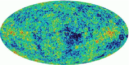
Figure 1: A sky map of CMB anisotropies measured by WMAP (Bennett et al. 2003).

2 Gravitational Lensing: Revealing the Dark Side

Although it is undoubtedly important to reveal the nature of dark matter, the main problem lies in the fact that dark matter is dark, i.e., it cannot be observed by usual methods. However, there is one way to probe the distribution of dark matter directly — gravitational lensing.

General relativity predicts that gravitational fields around massive objects, such as galaxies and clusters of galaxies, distort space-time and curve passing light rays. This phenomenon is called gravitational lensing. Gravitational lensing is sensitive only to the intervening mass, whether dark or luminous, thus is a powerful probe of the distribution of dark matter. If the gravitational fields are very strong, they can bend light rays so much that light can take different paths to the observer. In this case, we observe multiple images or highly distorted image of a distant source. Such drastic phenomena are called strong lensing. On the other hand, even if the gravitational fields are not so strong, they can be detected through systematic distortions of background galaxies. This is called weak lensing. Now both strong and weak lensing are indispensable tools for cosmology.

Historically, it was Einstein (1936) who first predicted strong lensing phenomena. He calculated formation of multiple images due to a foreground star, but in the paper it was concluded that “there is no hope of observing this phenomenon directly”. Zwicky (1937a, b) pointed out that the phenomena are more likely to be observed if we consider a foreground galaxy rather than star. However, it was still premature for strong lensing to be observed.

At long last, strong gravitational lensing was first discovered by Walsh, Carswell, & Weymann (1979). They showed that twin quasars Q0957+561A, B have almost the same spectra, and concluded that they are likely to be gravitational lensing. After that, $\sim 80$ gravitationally lensed quasars have been found so far. The first gravitationally lensed arc was also found in a rich cluster A370 (Lynds & Petrosian 1986; Soucail et al. 1987), and $\sim 40$ giant arcs have been detected in rich clusters. Therefore, strong gravitational lensing is now practically useful tool to explore the dark side of the universe.

For weak lensing signal, i.e., small systematic distortions of galaxies in response to the foreground mass distributions, to be detected, many background galaxies are needed to reduce the intrinsic ellipticities. Such weak lensing signal was first detected by Tyson, Wenk, & Valdes (1990) by make use of a high surface density of faint blue galaxies (Tyson 1988). Now weak lensing is one of the most popular method to study clusters of galaxies. In addition, the weak lensing signal due to large-scale structure also has been detected (van Waerbeke et al. 2000; Bacon, Refregier, & Ellis 2000; Wittman et al. 2000) and is now regarded as a powerful tool to study the large-scale structure of the universe.

In summary, gravitational lensing can be a powerful tool to study the distribution of dark matter which is not seen with usual methods.

3 Lensed Arcs and Quasars: Complementary Probes

In this thesis, we study strong gravitational lenses as a test of the CDM paradigm. We use strong lensing because it is sensitive to mass distributions at innermost regions of dark halos, and the mass distributions at the regions are particularly sensitive to the nature of dark matter. To probe mass distributions of dark halos, we focus on lensing by clusters of galaxies. In practice, effects of baryonic infall are expected to be small in clusters, compared with galaxies where inner structures are significantly affected by baryon cooling.

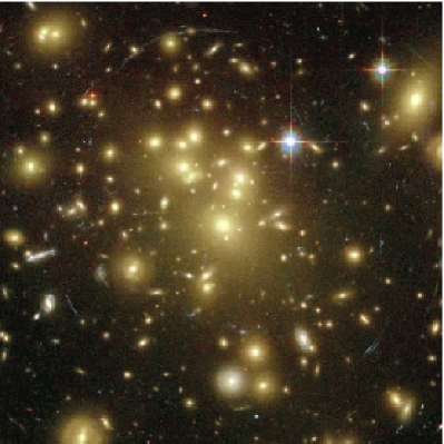
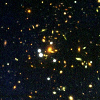
Figure 2: Left: Image of galaxy cluster Abell 1689, taken with Advance Camera for Surveys (ACS) of Hubble Space Telescope (HST). Many (curved) lensed galaxies are seen around the cluster. Taken form a webpage at http://antwrp.gsfc.nasa.gov/apod/ap030109.html. Right: First discovered gravitationally lensed quasar due to a cluster of galaxies. Four images around the center of the cluster represent the quadruple lensed images of a quasar. See Chapter 6 for details.

There are two types of strong gravitational lensing due to clusters of galaxies: lensed arcs and quasars (see Figure 2). The differences of these are summarized in Table 1. The most notable difference is the selection of lenses. For instance, in lensed quasar surveys one first identifies source quasars and then checks whether they are lensed, while in searching for lensed arcs one selects massive clusters and then searches for lensed arcs in them. In other words, surveys for arcs are biased toward high mass concentrations, while lensed quasars probe random lines of sight. Clusters selected by the presence of lensed quasars could, therefore, differ from those selected as having giant arcs. In addition, there are many differences between lensed arcs and quasars. For instance, sources of lensed arc systems are high-$z$ galaxies, which are extended and have poorly known source population (e.g., luminosity function). While the complexity of lensed arcs offers detailed constraints on the lens potential, the simplicity of lensed quasar systems can be an advantage because there is no confusion from unrelated background objects. Lensed quasars also make it easier to measure the source redshift and convert from dimensionless lensing quantities to physical units. The main disadvantage of lensed quasars is that such lens systems are quite rare due to the sparseness of quasars. In short, these two types of strong lensing, i.e., lensed arcs and quasars, have many different characteristics, and hence the conclusion would be much more robust when these complementary probes yield the similar results.

Lensed Arcs		Lensed Quasars
Lens-selected	Selection	Source-selected
Extended source	Source size	Point source
Less known	Source population	Well known
Difficult	Source-$z$ estimation	Easy
Difficult	Image identification	Easy
Not variable	Time-variability	Variable
(Mostly) Massive	Mass of lens cluster	Small – Massive
$\sim 40$ (giant arcs)	Observed number	1

Table 1: Comparison of two types of cluster-scale strong lensing; lensed arcs and lensed quasars.

In this thesis, we concentrate our attention on the statistics of strongly lensed arcs and quasars using the semi-analytic method that we developed. Why statistics? Statistics allow us to probe the mean mass distributions of clusters. Although individual modeling of lensing clusters can measure their mass distributions precisely, it may suffer from the special selection function and the scatter around the mean mass distribution. In addition, individual mass modeling sometimes confronts difficulties including uncertainties of the center of the mass distribution and the degeneracy between the ellipticity and central concentration. Why analytic approach? It is quite demanding for the numerical simulations to resolve the precise inner structure of lensing halos while keeping the reasonable number of those objects sufficient for statistical discussion. Moreover, an analytic approach has advantages of the ease of taking the selection function into account and the ability to clarify the key ingredients which dominate the statistics.

4 Organization of the Thesis

Part of this thesis is based in the published work (Oguri, Lee, & Suto 2003e, 2004a; Oguri & Keeton 2004c). This thesis is organized as follows.

In Chapters 1 and 2, we review the current status of the CDM model. First, in Chapter 1 we show how successful the standard model is. We review important cosmological observations to see how well the cosmology has converged toward a “concordance” model. In Chapter 2, in contrast, we see that the CDM model has difficulties to overcome; we summarize structures of dark halos in the CDM model and their difficulties in comparing with observations.

Chapter 3 is devoted to present the triaxial dark halo model and its lensing properties which we adopt in the thesis. Specifically, we review the triaxial model presented by Jing & Suto (2002), and then we study their lensing properties, such as convergence and deflection angles.

Our main work is presented in Chapters 4-6. First we explore arc statistics. We compute the numbers of arcs and compare them with observations in Chapter 4. Next we study lensed quasars. In Chapter 5, we theoretically predict the probabilities and image multiplicities of large-separation lensed quasars. Then we search for such lensed quasars from the Sloan Digital Sky Survey (SDSS) data and discover the first one, SDSS J1004+4112, which is shown in Chapter 6. Implications of the discovery are also shown in this Chapter.

Finally, we draw our conclusion in Chapter 7.

Chapter 1 A “Concordance” Model of Cosmology

1 The Case for a Flat Universe with Dark Matter and Dark Energy

Once we accept the cosmological principle (i.e., homogeneous and isotropic universe) as well as general relativity, the evolution of our universe is governed by the Friedman equation which is derived by solving the Einstein equation (see Appendix 8). One of the most fundamental parameters in this equation is the curvature of the universe. The curvature has attracted many attentions because it is (partly) related to fundamental questions about our universe: Is the universe finite or infinite? Or, is it expanding forever or not?

Other important parameter is the density content of the universe. The most surprising fact we have learned from cosmology is that the universe is dominated by two unknown components: Dark matter and dark energy. Dark matter is a non-relativistic matter component and is thought to be non-baryonic. Dark energy is a energy component which accelerates the expansion of the universe. In this section we review the observational case for a flat universe with the energy components dominated by dark matter and dark energy.

1 Flat Universe

Whether our universe is flat or not has been debated for a long time. Some theorists have claimed that the universe is likely to be flat, because the flat universe is most unlikely: If we consider the universe consists of ordinary matter only, then the evolution of the curvature term becomes

$$\Omega_{K}(a)=\Omega_{M}(a)-1=\frac{\Omega_{K}a^{-2}}{H^{2}(a)/H_{0}^{2}}\propto a,$$ (1)

during the matter dominated era ($H^{2}(a)\propto a^{-3}$). Therefore, if the universe is not a flat universe, then the curvature had to be fine-tuned in the very early universe, because we know that the curvature term is, if it exists, close to unity $\Omega_{K}={\mathcal{O}}(1)$ from the fact that $\Omega_{M}={\mathcal{O}}(1)$. But it is also extremely unlikely that $\Omega_{K}(a)$ is exactly zero, because the above discussion suggests that such a spacetime is unstable. This problem is known as flatness problem.

One possible solution of this flatness problem is to consider an accelerating phase in the early universe. The inflationary scenario, in which the universe experiences acceleration due to the domination of the potential energy of a scalar field (called inflaton because it is still unclear what the scalar field is), gives a natural explanation of why the universe is (nearly) flat. This is easily understood as follows. From the fact that the potential energy density of a scalar field does not change as the universe expands, we derive $H(a)\sim{\rm const.}$ and $a\propto e^{Ht}$ during inflation (see also §3). In this case, equation (1) reduces to $\Omega_{K}(a)\propto a^{-2}$, which means that $|\Omega_{K}(a)|$ rapidly decreases during inflation.

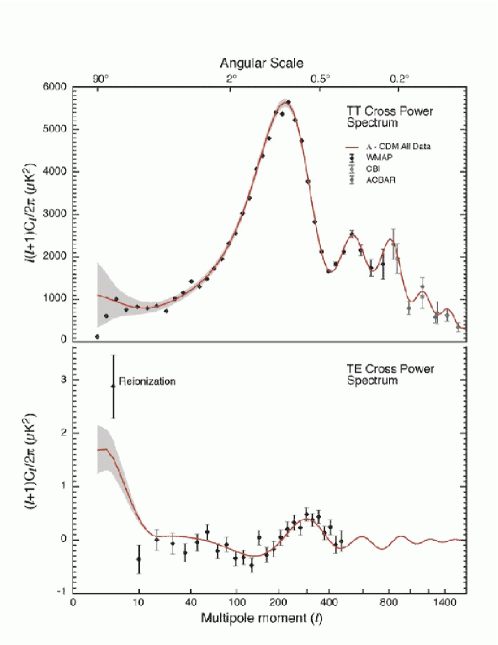
Figure 1: Top: WMAP temperature angular power spectrum is compared with best-fit Lambda-dominated CDM model. The small-scale data from ACBAR (Kuo et al. 2004) and CBI (Pearson et al. 2003) are also shown. Bottom: Temperature-polarization cross-power spectrum is compared with best-fit Lambda-dominated CDM model. Strong correlation seen at very large scale is generated by the reionization of the universe. This Figure is taken from Bennett et al. (2003).

While these progresses on theoretical understanding of the flatness of the universe, observational case for the flat universe had not been so strong. However, observations of CMB anisotropies changed the situation: The angular scale of peaks in angular power spectrum of CMB can be an excellent indicator of the curvature of the universe because of the following two reasons; (1) physical scale of the peak is determined by the sound horizon scale at the decoupling, which depends on the cosmological parameters only weakly; (2) on the other hand, the angular diameter distance from us to the last scattering surface of CMB strongly depends on the curvature of the universe. The measurements of the first peak has been reported by many groups such as BOOMERanG (de Bernardis et al. 2000), MAXIMA (Hanany et al. 2000), DASI (Halverson et al. 2002), and WMAP (Bennett et al. 2003). All these groups claimed the detection of the peak at multipole moment $l\sim 200$, which is roughly corresponding to $1^{\circ}$ scale, indicating that the universe is (nearly) flat. Figure 1 shows angular power spectrum measured by WMAP (Bennett et al. 2003). A distinct peak around $l=200$ constrains the curvature of the universe to be $-0.02<\Omega_{K}<0.08$ (95% C.L.) if we include a weak prior $h>0.5$ (Spergel et al. 2003).

2 Dark Matter

Dark matter is a dust component ($w=0$) which does not interact (or only weakly interacts) electromagnetically. Dark matter is first proposed by Zwicky (1933): He estimated the mass of the Coma cluster from peculiar velocities of galaxies in the cluster and found that it is 400 times larger than that estimated by adding up all of the galaxy masses. Although the idea had not been taken seriously, it was revived in 1970’s and 1980’s. For instance, Rubin & Ford (1970) found that the velocities of the ionized clouds in the Andromeda galaxy do not decrease with increasing distance from the center and that the extra mass has to be in the outer part of the galaxy; Rubin et al. (1985) confirmed that the phenomena is commonly seen in spiral galaxies; Ostriker & Peebles (1973) pointed out that the spherical halo component is needed to stabilize the flatten disk galaxy. From these studies, people began to accept the idea of dark matter.

Now, one of the strongest case for dark matter comes from observations of cluster of galaxies. First of all, clusters of galaxies are X-ray luminous; thus the mass of the cluster can be estimated under the assumption of hydrodynamic equilibrium, which turns out to be much larger than mass of the visible matters (i.e., gas + stars). For instance, White et al. (1993) obtained the fraction of the visible mass in Coma cluster to be $M_{b}/M_{\rm tot}\simeq 0.01+0.05h^{-3/2}$. This means that the cluster of galaxies must be dominated by invisible dark matter. More direct evidence is offered by gravitational lensing, because it allows one to measure the mass of clusters directly. Squires et al. (1996) estimated an upper bound for the fraction of the gas mass to be $M_{\rm gas}/M_{\rm tot}<(0.04\pm 0.02)h^{-3/2}$ using weak lensing method. Both X-ray and lensing data consistently show that visible matters cannot account for the total masses of clusters of galaxies. Given the total baryon density of $\Omega_{b}h^{2}\sim 0.02$ (see §2), these results imply $\Omega_{M}\sim 0.3$.

Another evidence for the existence of dark matter is the CMB anisotropy. The existence of non-baryonic dark matter can be concluded from the detailed observations of CMB angular power spectrum as follows; (1) relative peak heights of even peaks (second peak, fourth peak, ..) to those of odd peaks (first peak, third peak, ..) tightly constrain the baryon matter density $\Omega_{b}h^{2}$; (2) the amount of boost of angular power spectrum around first peak is caused by the potential decay during radiation dominated era (early integrated Sachs-Wolfe effect), and therefore is sensitive to matter-radiation equality, i.e., $\Omega_{M}h^{2}$. The detailed angular power spectrum measured by WMAP revealed that $\Omega_{M}h^{2}$ is about six times larger than $\Omega_{b}h^{2}$ (Spergel et al. 2003). This indicates that the most of the matter in the universe should be non-baryonic and dark. In addition, the need for dark matter can be also said from much simpler discussions; the CMB anisotropies of the order of $10^{-5}$ cannot be achieved from the baryonic matter only because of the slow linear growth rate $D_{+}\propto a$ combined with the decoupling at $z\sim 10^{-3}$. For the enough amounts of non-linear objects to be observed today, we need an energy component which was not coupled to baryon-photon fluid before decoupling and had already grown to much larger than $10^{-5}$ at the last scattering surface.

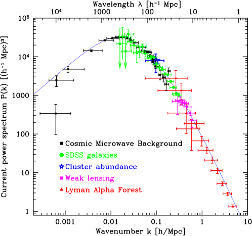
Figure 2: Comparison of several comparisons on the power spectrum. The line is the CDM prediction with $\Omega_{M}=0.28$, $h=0.72$, and $\Omega_{b}/\Omega_{M}=0.16$. This Figure is taken from Tegmark et al. (2004).

Dark matter candidates can be classified according to their collisionless damping (freestreaming) scales. If we regard massive neutrinos ($m_{\nu}\gtrsim 10{\rm eV}$) as dominant component of dark matter, then they were relativistic until the horizon scale of $\sim$Mpc; therefore fluctuations below $\sim$Mpc were smoothed out due to their relativistic motions. Such dark matter is called hot dark matter (HDM). On the other hand, one can consider a possibility of very massive dark matter so that it became non-relativistic long time ago; this time collisionless damping scale will be much smaller than important scales for structure formation. This is called cold dark matter (CDM). There is also a possibility of warm dark matter (WDM) which has collisionless damping scale of $\sim$kpc. The difference of these dark matter models is well understood by their power spectra (see Appendix 9). Now observations support the cold dark matter model; Figure 2 shows the comparison of observed power spectrum with cold dark matter predictions. They are in good agreement at $\gtrsim$Mpc scales. Therefore now it is believed that most of dark matter is non-baryonic and cold.

3 Dark Energy

Dark energy is an unknown energy component which accelerates the expansion of the universe. In terms of the equation of state, accelerating universe is possible if the (effective) equation of state satisfies $w<-1/3$. Cosmological constant, which is one of candidates for dark energy, is first proposed by Einstein to make the universe static. However, soon after the proposal Einstein discarded the idea of cosmological constant because it turned out that the universe is not static but expanding (he regretted the idea as “the biggest blunder of my life”).

Since then, cosmological constant had not been taken seriously. However things began to change in 1990’s. A reason to invoke the cosmological constant is the age of the universe; cosmological constant was needed to reconcile the possible large Hubble constant (e.g., Aaronson et al. 1986; Tonry 1991) with the lower limit of the cosmic age inferred from the evolution of the globular cluster (e.g., Vanden Berg 1983). In addition, the best fit of the number count of faint galaxies was also obtained only with a cosmological constant (Fukugita et al. 1990b). Moreover, cosmological constant was favorable from the theoretical point of view because a flat universe, which is predicted by inflation model, can be reconciled with the observed low-matter universe if we assume the large cosmological constant (see §2).

However, the idea of cosmological constant included several difficulties such as coincidence problem (“why now?” problem); that is, it is highly unnatural for the density of cosmological constant to be comparable to that of matter components today, given the different dependence of densities on the scale factor $a$ ($\propto a^{-3}$ for matter and $\propto a^{0}$ for cosmological constant). This means that the cosmological constant must be fine-tuned in order to be important in the current universe. One solution is to consider a dynamical scalar field on the analogy of the inflation model (often called quintessense; Caldwell, Dave, & Steinhardt 1998). The energy and pressure density of a scalar field $\Phi$ are

$$\rho_{\Phi}=\frac{1}{2}\dot{\Phi}^{2}+V(\Phi),$$ (2)

$$p_{\Phi}=\frac{1}{2}\dot{\Phi}^{2}-V(\Phi),$$ (3)

where $V(\Phi)$ denotes the potential of the scalar field. Hence, $w_{\Phi}=p_{\Phi}/\rho_{\Phi}\sim-1$ can be achieved if the potential term dominates. The advantage of this model is that there does exist a model in which the solution is attractive, i.e., it is asymptotic solution for a broad range of initial conditions (e.g., Ratra & Peebles 1988). Observationally the model may be discriminated to cosmological constant because the effective equation of state $w_{\Phi}$ is not necessarily $w_{\Phi}\sim-1$, and also is not necessarily time-independent. Now the energy components with the negative equation of state are collectively called dark energy; it includes cosmological constant, dynamical scalar field, and topological defects which also have the negative equation of state.

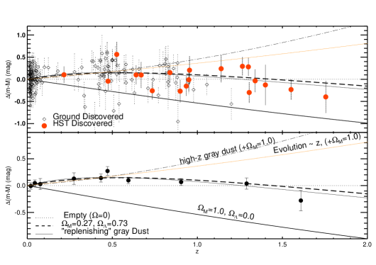
Figure 3: The Hubble diagram of type-Ia supernovae. $\Delta(m-M)$ denotes the distance modulus relative to an empty universe. The data are in good agreement with the cosmological constant dominated model; $\Omega_{M}=0.23$ and $\Omega_{\Lambda}=0.73$. As seen, the data exclude simple gray dust model and evolution model, though “replenishing” (i.e., physical density of dust is constant) dust model can account for the observed behavior. This Figure is taken from Riess et al. (2004).

The most “direct” evidence of dark energy is thought to be distant type-Ia supernovae. Empirically, absolute magnitudes of type-Ia supernovae have turned out to be almost constant with small dispersion. Therefore, once the absolute magnitudes are calibrated in a local universe, then type-Ia supernovae can be a distance indicator at high-$z$ ($z\sim 1$) universe. Actually, two groups independently showed that the apparent magnitude at $0.1\lesssim z\lesssim 1$ is fainter than empty universe, and that we need dark energy component to account for the observed magnitude-redshift relations (Riess et al. 1998; Perlmutter et al. 1999). Now the case is much stronger because it has turned out that at $z\gtrsim 1$ supernovae become brighter, which indicates that the universe was decelerating in the past (Riess et al. 2001, 2004). This different behavior before and after $z\sim 1$ excludes many of alternative explanations of the observed supernovae magnitude-redshift relations (see Figure 3).

Gravitational lensing statistics are known to offer similar cosmological test. The lensing probability is sensitive to the volume of the universe, so it can be used to place interesting constraints on the cosmological constant $\Omega_{\Lambda}$ (Turner 1990; Fukugita, Futamase, & Kasai 1990a; Kochanek 1996; Chiba & Yoshii 1999; Chae et al. 2002; Mitchell et al. 2004). For instance, Chae et al. (2002) derived the constant on the cosmological constant assuming the flat universe as $\Omega_{\Lambda}=0.69^{+0.14}_{-0.27}{}^{+0.10}_{-0.12}$ (68% C.L.).

Another evidence is again offered by CDM anisotropies. First, as discussed before, the peak position and peak height of first peak strongly constrain $\Omega_{K}$ and $\Omega_{M}h^{2}$, respectively. Even if we combine these constraints, however, the strong degeneracy between $\Omega_{M}$ (or $\Omega_{\Lambda}$) and $h$ still remains. This degeneracy is known as geometric degeneracy (Efstathiou & Bond 1999). However, if we add one more constrain, such as the distance ladder, supernova Ia, or power spectrum, as a prior, then we obtain the finite cosmological constant at high statistical significance (see, e.g., Spergel et al. 2003). Although the above example is indirect, more direct evidence has been obtained through positive correlation between CDM anisotropies and galaxies distribution which is caused by a potential decay in a dark energy dominated universe (late integrated Sachs-Wolfe effect; Fosalba, Gaztañaga, & Castander 2003; Boughn & Crittenden 2004; Afshordi, Loh, & Strauss 2004; Nolta et al. 2004; Scranton et al. 2004).

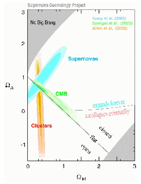
Figure 4: Three independent constraints on cosmological parameters projected in the $\Omega_{M}$-$\Omega_{\Lambda}$ plane. “CMB” is constraints from CMB anisotropy observed by WMAP (Spergel et al. 2003). “Supernovae” denote results of type-Ia supernovae observations by Knop et al. (2003). Constraints denoted by “Clusters” come from X-ray measurements of distant clusters (Allen, Schmidt, & Fabian 2002). It is surprising that these three independent observations are well explained by a model with $\Omega_{M}\sim 0.3$ and $\Omega_{\Lambda}\sim 0.7$. This Figure is taken from http://www-supernova.lbl.gov/

2 A “Concordance” Model

Parameter	Fiducial	Meaning
$\Omega_{M}(=1-\Omega_{\Lambda})$	$0.3$	Current matter density of the universe (CDM$+$baryon)
$\Omega_{b}$	$0.04$	Current baryon density of the universe
$h$	$0.7$	The Hubble constant in units of $100{\rm km\,s^{-1}\,Mpc^{-1}}$
$n_{s}$	$1.0$	Index of the primordial power spectrum
$\sigma_{8}$	$0.9$	Normalization of the density fluctuation

Table 1: Model parameters of the concordance model described in §2. The entry “Fiducial” denotes the value we adopt in this thesis (unless otherwise specified).

As discussed in the previous section, now there are lots of evidences that the universe is flat and dominated by dark matter and dark energy. As shown in Figure 4, several independent observations point a model with $\Omega_{M}\sim 0.3$ and $\Omega_{\Lambda}\sim 0.7$. This remarkably successful model is now called a “concordance” model. Although the definition of the concordance model may not be unique, we define it by the followings:

• The evolution of the universe is governed by general relativity. The topology of the universe is simple.

• The universe is flat ($E^{3}$). The matter components are baryon, dark matter, and dark energy. We also assume the densities of radiation components of photons and neutrinos as inferred from the CMB temperature and that calculated from the standard thermal history. We assume the three massless species of neutrinos.

• We assume the adiabatic primordial fluctuations. The fluctuations obey the Gaussian statistics. The primordial power spectrum can be described by a power law, $P_{i}(k)\propto k^{n_{s}}$.

• The dark matter is cold, i.e., collisionless damping of the power spectrum due to freestreaming is negligible.

• The equation of state $w$ of dark energy is assumed to be $w=-1$ and time-independent.

The assumption of the adiabatic Gaussian primordial fluctuations are supported by the high-resolution measurements of CMB anisotropies (Spergel et al. 2003; Komatsu et al. 2003; Peiris et al. 2003). In particular, large-scale temperature-polarization anti-correlation (see Figure 1) offers a strong evidence for adiabatic superhorizon fluctuations (Peiris et al. 2003). Theoretically, such fluctuations can be explained in the simple inflation model, in which the fluctuations are generated by quantum fluctuations of the inflaton field.

We assume the above concordance model throughout the thesis. In this model, the number of basic (independent) parameters is only five, which are listed in Table 1. We also show fiducial values of these parameters which will be adopted in this thesis. In the next section, we will see that the adopted cosmological parameters do explain so many observations. To see how successful it is, we show an example; 1,348 data points of the angular power spectrums (both temperature-temperature and temperature-polarization) measured by WMAP (see Figure 1) are well fitted by the concordance model (plus one more parameter, optical depth $\tau$) which contains only 6 parameters. The reduced chi-square is $\chi^{2}/{\rm dof}=1.066$ for 1,342 degrees of freedom (Spergel et al. 2003).

3 Constraints on Model Parameters

1 Current Matter Density $\Omega_{M}$

Method	$\Omega_{M}$: Mean (68% C.L.)	Ref.
Type-Ia supernovae	$0.29^{+0.05}_{-0.03}$	1
Lensing statistics	$0.31^{+0.27}_{-0.14}{}_{-0.10}^{+0.12}$	2
Cluster X-ray gas mass (+HST $h$, BBN)	$0.30^{+0.04}_{-0.03}$	3
Galaxy power spectrum (+HST $h$)	$0.36\pm 0.07$	4
CMB anisotropy	$0.29\pm 0.07$	5

Table 2: Recent $\Omega_{M}$ determinations.
      Ref. — (1) Riess et al. 2004; (2) Chae et al. 2002; (3) Allen et al. 2002; (4) Pope et al. 2004; (5) Spergel et al. 2003

As discussed before, type-Ia supernovae and lensing statistics offer good tests for $\Omega_{\Lambda}$ (and also $\Omega_{M}$). Assuming a flat universe, Riess et al. (2004) derived constraints on $\Omega_{M}$ with 10% accuracy; $\Omega_{M}=0.29^{+0.05}_{-0.03}$. Chae et al. (2002) constrained $\Omega_{M}$ from the lensing statistics of flat-spectrum $\sim$10,000 radio sources; $\Omega_{M}=0.31^{+0.27}_{-0.14}{}_{-0.10}^{+0.12}$ (stat.+syst.). Note that both methods might suffer from systematic effects, such as intergalactic dusts and evolution of the number density of galaxies. Nevertheless, the excellent agreement suggests that the result of $\Omega_{M}\sim 0.3$ seems quite robust.

Clusters of galaxies also can be used to put tight constraints on $\Omega_{M}$. Allen et al. (2002) derived $\Omega_{M}$ using the (apparent) redshift evolution of cluster gas-mass fraction, which is the method described by Sasaki (1996), and found that $\Omega_{M}=0.30^{+0.04}_{-0.03}$, once the priors on $h$ and $\Omega_{b}h^{2}$ are taken into account (see §2 and §3). The result shows an excellent agreement with type-Ia supernovae and lensing statistics.

Another method to determine $\Omega_{M}$ is the galaxy power spectrum (see also Appendix 9). Usually the power spectrum has a characteristic scale corresponding to the horizon size at matter-radiation equality $\lambda_{\rm eq}$, because of the following reason. Fluctuations with scales larger than $\lambda_{\rm eq}$ enter the horizon when the universe is matter dominant. Such fluctuations grow as soon as they enter the horizon. Therefore the power spectrum at those scales does not change the shape. On the other hand, fluctuations with scales less than $\lambda_{\rm eq}$ enter the horizon when the universe is still radiation dominant. Fluctuations in that epoch do not grow in practice because of the rapid expansion of the universe. Smaller fluctuations suffer from the longer period of the suppression, and result in the modification of the spectrum as $P(k)\sim P_{i}(k)k^{-4}$. Therefore, the measurement of this characteristic scale will constrain the matter-radiation equality epoch and thus $\Omega_{M}h$. If combined with constraints on $h$, this allows one to determine $\Omega_{M}$. Pope et al. (2004) derived $\Omega_{M}=0.36\pm 0.07$ based on the galaxy power spectrum measured by the SDSS.

Finally, we mention constraints from CMB anisotropies. Even CMB alone does constrain $\Omega_{M}$ if we assume a flat universe, by combining the precise peak position (determined by $\Omega_{M}h^{3.4}$) and early ISW constraints on $\Omega_{M}h^{2}$. From the WMAP measurements, Spergel et al. (2003) constrained $\Omega_{M}=0.29\pm 0.07$ assuming the concordance model.

These recent determinations are summarized in Table 2. It is surprising that all measurements are consistent with $\Omega_{M}=0.3$. The matter density can be also determined from e.g., cluster abundances and weak lensing, but we use these to constrain $\sigma_{8}$ because of tight correlation between $\Omega_{M}$ and $\sigma_{8}$ in these measurements.

2 Current Baryon Density $\Omega_{b}$

Method	$\Omega_{b}h^{2}$: Mean (68% C.L.)	Ref.
Big bang nucleosynthesis (D)	$0.0214\pm 0.0020$	1
Big bang nucleosynthesis (7Li)	$0.006-0.016$ (95%)	2, 3
CMB anisotropy	$0.0237^{+0.0013}_{-0.0012}$	4
Ly$\alpha$ forests	$0.02\pm 0.01$	5

Table 3: Recent $\Omega_{b}h^{2}$ determinations.
      Ref. — (1) Kirkman et al. 2003; (2) Ryan et al. 2000; (3) Coc et al. 2002; (4) Spergel et al. 2003; (5) Scott et al. 2000

The baryon density $\Omega_{b}$ is usually constrained in the combination of $\Omega_{b}h^{2}$. Therefore, in this subsection we review current determinations of $\Omega_{b}h^{2}$ rather than $\Omega_{b}$.

Traditionally $\Omega_{b}h^{2}$ has been determined by the Big Bang Nucleosynthesis (BBN). Since the light element abundances produced in the early universe depends only on baryon-to-photon ratio $\eta$ and thus on $\Omega_{b}h^{2}$, by observing the primordial light element abundances, such as ⁴He, D, and ⁷Li, one can determine $\Omega_{b}h^{2}$. Among the light elements, D is perhaps the best element to constrain $\Omega_{b}h^{2}$ because of the small uncertainties. For instance, Kirkman et al. (2003) combined absorption systems of five quasars, and derived $\Omega_{b}h^{2}=0.0214\pm 0.0020$. On the other hand, Coc et al. (2002, see also ) determined the baryon density using ⁷Li as $\Omega_{b}h^{2}=0.006-0.016$ (95%). This value seems much lower than that derived from D.

Another precise measurement comes from CMB anisotropies. As discussed, relative peak heights of even peaks to those of odd peaks constrain $\Omega_{b}h^{2}$. This method is quite robust because no other parameters can mimic such behavior. Using up to the third peak, WMAP data only determined $\Omega_{b}h^{2}=0.0237^{+0.0013}_{-0.0012}$ (Spergel et al. 2003).

The ionizing background $J_{H}$ also allows us to determine $\Omega_{b}h^{2}$. This is because the Ly$\alpha$ optical depth, which can be measured from the transmission power spectrum of Ly$\alpha$ forest, is proportional to $(\Omega_{b}h^{2})^{2}/J_{H}$. For instance, the ionizing background from the proximity effect measured by Scott et al. (2000) implies $\Omega_{b}h^{2}=0.02\pm 0.01$.

These recent determinations are summarized in Table 3. It is indeed striking that BBN and CMB are consistent with each other ($\Omega_{b}h^{2}\sim 0.02$, which implies $\Omega_{b}\sim 0.04$ if we adopt $h\sim 0.7$), since they probe baryon densities at totally different epochs ($t\sim 3$ minutes for BBN and $t\sim 4\times 10^{5}$ years for CMB). However, it should be kept in mind that ⁷Li seems inconsistent with the other results. This discrepancy might be ascribed to the uncertainties of nucleon reaction rate (Coc et al. 2004) or the baryon input after BBN (Ichikawa, Kawasaki, & Takahashi 2004).

3 The Hubble Constant $h$

Method	$h$: Mean (68% C.L.)	Ref.
HST Key Project	$0.72\pm 0.03\pm 0.07$	1
Cluster SZ + X-ray	$0.60^{+0.04}_{-0.04}{}^{+0.13}_{-0.18}$	2
Gravitational lens time delay	$0.48\pm 0.02$	3
CMB anisotropy	$0.72\pm 0.05$	4

Table 4: Recent Hubble constant determinations.
      Ref. — (1) Freedman et al. 2001; (3) Reese et al. 2002; (3) Kochanek 2002a; (4) Spergel et al. 2003

The Hubble constant has been regarded as the most important cosmological parameter because it is directly related with the distances to the objects (and the size of the universe). The traditional way to measure the Hubble constant is the distance ladder. Cepheid distances are used to calibrate the second distance indicators such as type Ia supernovae, Tully-Fisher relation, fundamental plane, type II supernovae, and surface brightness fluctuations. The HST Key Project (Freedman et al. 2001) is aimed to find many Cepheids to calibrate the secondary distances. They concluded that the Hubble parameter is determined with the accuracy of 10%, $h=0.72\pm 0.03\pm 0.07$ (stat.+syst.).

Since the above method can measure only the local ($z\lesssim 0.1$) value of the $h$, it is important to check it from independent direct methods. The distant clusters offer one of such methods. The flux of Sunyaev-Zel’dovich effect in a cluster is $\propto n_{e}T_{e}$, where $n_{e}$ and $T_{e}$ are electron number density and temperature, while X-ray flux is $\propto n_{e}^{2}T_{e}^{1/2}$. From these different dependences on $n_{e}$, we can determine the luminosity distance to the cluster. Although at high redshift ($z\sim 1$) derived Hubble constant is somewhat sensitive to assumed cosmological model, by assuming $\Omega_{M}=0.3$ and $\Omega_{\Lambda}=0.7$, Reese et al. (2002) determined $h=0.60^{+0.04}_{-0.04}{}^{+0.13}_{-0.18}$ (stat.+syst.) from 18 distant clusters.

Another direct method to probe $h$ is gravitational lens time delays, because time delays are dimensional quantity (i.e., $\Delta t\propto h^{-1}$) while other observables (image separations, etc.) are dimensionless. Kochanek (2002a) applied this method to five quasar lens systems, and derived the value of $h=0.48\pm 0.02$ assuming the singular isothermal mass distribution of the lensing galaxy. The value is significantly lower than those derived from the other method. However, the important point is that there is a strong degeneracy between mass distributions in the lens galaxies and the derived $h$. Thus, this low value may be interpreted that the lens galaxy is more complicated than the simple singular isothermal mass distribution.

CMB observations give the value of $h$ by combining the early ISW and the peak position, as discussed in §1. Spergel et al. (2003) constrained $h=0.72\pm 0.05$ based on the WMAP measurements.

These recent determinations are summarized in Table 4. The value of $h$ is also basically converging. The values derived from clusters and gravitational lens time delays seem lower than the others, but those methods actually may be dominated by systematic effects. Thus, more and more theoretical and observational studies are needed to reduce these systematic uncertainties (not statistical uncertainties).

4 Index of the Primordial Power Spectrum $n_{s}$

Data	$n_{s}$: Mean (68% C.L.)
WMAP	$0.99\pm 0.04$
WMAPext	$0.97\pm 0.03$
WMAPext+2dF	$0.97\pm 0.03$
WMAPext+2dF+Ly$\alpha$	$0.96\pm 0.02$

Table 5: Index determinations presented by Spergel et al. (2003). “ext” denotes small-scale CMB data from ACBAR (Kuo et al. 2004) and CBI (Pearson et al. 2003). “2dF” is the power spectrum measurements by two-degree Field system (Percival et al. 2001). The measurements of Ly$\alpha$ power spectrum (Croft et al. 2002; Gnedin & Hamilton 2002) are denoted by “Ly$\alpha$”. See Figures 1 and 2 to understand which data corresponds to which scales.

To determine $n_{s}$, it is essential to see superhorizon fluctuations which have not been affected by any physical processes after the fluctuation generation. Therefore, here we restrict our attention on constraints from the CMB anisotropies (plus some other data sets).

The constraints from WMAP (Spergel et al. 2003) are summarized in Table 5. We show how the results are changing as we add small-scale data sets. First of all, the results indicate that the index is very close to 1. This is indeed consistent with what inflation model did predict. Basically, the small deviation from $n_{s}=1$ and its scale-dependence reflects the shape of potential during the inflation. Therefore, in principle we can reconstruct the potential of inflation from the precise measurement of the primordial power spectrum. Peiris et al. (2003) showed that the current date are not so good as to constrain inflation models severely, but do have an ability to reject some of inflation models.

5 Normalization of the Density Fluctuation $\sigma_{8}$

Method	$\sigma_{8}$: Mean (68% C.L.)	$\Omega_{M}$ dependence	Ref.
Cluster (local)	$0.69\pm 0.04$	$(\Omega_{M}/0.3)^{-0.25}$	1
	$0.77\pm 0.04$	$(\Omega_{M}/0.3)^{-0.60}$ ?	2
	$0.68\pm 0.06$	$(\Omega_{M}/0.3)^{-0.60}$	3
	$0.74\pm 0.04$	$(\Omega_{M}/0.3)^{-0.60}$ ?	4
	$0.77\pm 0.07$	$(\Omega_{M}/0.3)^{-0.44}$	5
Cluster (high-$z$)	$0.92\pm 0.09$	$(\Omega_{M}/0.3)^{-0.14}$	6
	$1.04\pm 0.06$	$(\Omega_{M}/0.3)^{-0.00}$ ?	7
Weak lensing	$1.09\pm 0.12$	$(\Omega_{M}/0.3)^{-0.51}$	8
	$1.02\pm 0.16$	$(\Omega_{M}/0.3)^{-0.46}$	9
	$0.67\pm 0.10$	$(\Omega_{M}/0.3)^{-0.60}$	10
	$0.78^{+0.27}_{-0.12}$	$(\Omega_{M}/0.3)^{-0.37}$	11
	$0.97\pm 0.13$	$(\Omega_{M}/0.3)^{-0.68}$	12
	$0.72\pm 0.09$	$(\Omega_{M}/0.3)^{-0.49}$	13
	$0.71^{+0.06}_{-0.08}$	$(\Omega_{M}/0.3)^{-0.57}$	14
	$0.86^{+0.05}_{-0.07}$	$(\Omega_{M}/0.3)^{-0.52}$	15
	$0.94\pm 0.17$	$(\Omega_{M}/0.3)^{-0.44}$	16
CMB (WMAP)	$0.90\pm 0.10$	$\cdots$	17
CMB (WMAPext)	$0.80\pm 0.10$	$\cdots$	17

Table 6: Recent $\sigma_{8}$ determinations.
      Ref. — (1) Allen et al. 2003; (2) Pierpaoli et al. 2003; (3) Bahcall et al. 2003a; (4) Schuecker et al. 2003; (5) Seljak 2002; (6) Bahcall & Bode 2003b; (7) Komatsu & Seljak 2002; (8) Massey et al. 2004; (9) Rhodes et al. 2004; (10) Heymans et al. 2004; (11) Hamana et al. 2003; (12) Bacon et al. 2003; (13) Brown et al. 2003; (14) Jarvis et al. 2003; (15) Hoekstra, Yee, & Gladders 2002; (16) Refregier, Rhodes, & Groth 2002; (17) Spergel et al. 2003

The amplitude of current linear fluctuations within $8h^{-1}{\rm Mpc}$ sphere, $\sigma_{8}$, has been determined from cluster abundances, weak lensing surveys, and CMB anisotropies. Cluster abundances and weak lensing surveys are more direct methods in the sense that they probe current fluctuations at the scale near $8h^{-1}{\rm Mpc}$. On the other hand, from CMB anisotropies we know large-scale fluctuations at $z\sim 10^{3}$; therefore we have to extrapolate the result both in the scale and time. Usually, constraints from cluster abundances and weak lensing surveys show strong $\sigma_{8}$-$\Omega_{M}$ correlation, thus below we normalize the values to $\Omega_{M}=0.3$. Results are summarized in Table 6.

Since the mass function of clusters of galaxies is sensitive to density fluctuations, cluster abundances are powerful tool to determine $\sigma_{8}$. Weak lensing shear power spectrum (or shear 2-point correlation function) is also directly related with the matter power spectrum, thus it allows us to constrain $\sigma_{8}$. As seen in Table 6, however, different groups presented rather different values. Actually the differences are much larger than statistical errors, indicating that systematic errors may dominate. The source of the systematic effects is unknown, but it could be uncertainties (or inaccuracies) of the theoretical power spectrum (see Appendix 9). In cluster surveys, it is sometimes difficult to convert observable quantities (temperature, luminosity, richness, etc.) to masses of clusters. One of the biggest shortcomings in weak lensing surveys is that the constraints are dependent on the redshift distribution of the source galaxies which is quite hard to know from observations. Therefore, we conclude that the current constraints on the value of $\sigma_{8}$ are very roughly $0.7\lesssim\sigma_{8}\lesssim 1.0$.

It should be noted that cluster abundances at high-$z$ require significantly larger $\sigma_{8}$ ($\sigma_{8}\sim 1$) than those at local universe ($\sigma_{8}\sim 0.7$). While this discrepancy can be resolved by lowering $\Omega_{M}$ (see “$\Omega_{M}$ dependence” in Table 6), it might imply something beyond the concordance model; Oguri et al. (2003d) introduced decaying CDM model to resolve the discrepancy; Łokas, Bode, & Hoffman (2004) considered the dark energy model with $w\neq-1$ (see §4), and found that the data might be better explained.

Finally, we see constrains from CMB anisotropies. The result from WMAP alone is $\sigma_{8}=0.90\pm 0.10$ , and when we add small-scale CMB data sets it changes to $\sigma_{8}=0.80\pm 0.10$. In both cases, the results are roughly consistent with those of cluster abundances and weak lensing surveys.

4 Beyond the Concordance Model?

Although the concordance model has achieved remarkable success, the possibility that we will need the model beyond the concordance model in the future still remains. Below we pursuit some of the possibilities.

Dark Energy

We have already seen in §3 that the dynamical model is more natural than the cosmological “constant”. To discriminate these, it is important to determine the dark energy equation of state $w$: If it turns out that $w=-1$ and $w$ is time-independent, then the dark energy is likely to be the cosmological constant. If not, the accelerating universe might be caused by a scalar field. In this case, the degree of the deviation from $w=-1$ and its time evolution is directly related with the shape of the potential of the scalar field. Thus it is often said that the measurements of $w$ offer clues to the nature of dark energy.

Because of this importance, until now a number of methods are proposed to probe the dark energy equation of state (e.g., Matsubara & Szalay 2003; Jain & Taylor 2003; Blake & Glazebrook 2003; Cooray, Huterer, & Baumann 2004; Takahashi et al. 2004b) besides the methods described above. In addition, there are so many plans to catch up the nature of dark energy, such as SNAP which will determine $w$ with $\sim$5% accuracy.

However, the current status seems not so exciting: None of the results does require the dark energy with $w\neq-1$. For instance, assuming constant $w$ Spergel et al. (2003) concluded $w=-0.98\pm 0.12$ from the WMAPext+large scale structure data. Riess et al. (2004) derived $w=-1.02^{+0.13}_{-0.19}$ using type-Ia supernova data with a prior $\Omega_{M}=0.27\pm 0.04$. The data are also consistent with the static (i.e., time-independent) nature of dark energy. Thus the property of dark energy should be very close to that of the cosmological constant, even if it is not the cosmological constant.

Running Spectral Index

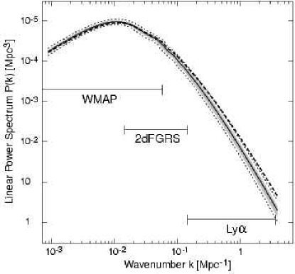
Figure 5: The fitted power spectrum by WMAP results. Shaded regions and dotted lines show the $1\sigma$ contours and $2\sigma$ limit for the running spectral index model. The dashed line is the best-fit power spectrum of the concordance model described in §2. This Figure is taken from Spergel et al. (2003).

The somewhat strange behavior seen in Table 5 is that the value of $n_{s}$ becomes smaller and smaller as we add more and more small-scale data. This may indicate that we need a new parameter beyond the concordance model.

Motivated by this, Spergel et al. (2003) considered a running spectral index model in which the primordial power spectrum is described by

$$P_{i}(k)=P_{i}(k_{0})\left(\frac{k}{k_{0}}\right)^{n_{s}+(1/2)dn_{s}/d\ln k\ln(k/k_{0})},$$ (4)

where $dn_{s}/d\ln k$ is a constant parameter which means the degree of running (recover power-law $P_{i}(k)$ when $dn_{s}/d\ln k=0$). They found $dn_{s}/d\ln k=-0.031^{+0.016}_{-0.017}$ from the combined data set (WMAPext+2dF+Ly$\alpha$). Thus the data favor (but not require) the running spectral index. See Figure 5 for the difference between the best-fits of the concordance model and running spectral index model. Theoretically, such running of the power spectrum can easily be achieved by taking account of the second-order slow-roll parameters (see Peiris et al. 2003).

One of the important consequence of the running spectral index model is significantly lower amplitudes of fluctuations on small scales (see Figure 5). This might be a good news for possible problems of CDM model on small scales (Chapter 2). However, things are more complicated; a simple extrapolation of the running spectral index to smaller scale cannot explain the early reionization found by the temperature-polarization cross-power spectrum at low-$l$ (Yoshida et al. 2003). Therefore, it is still unclear whether we really need the running spectral index or not.

Non-Gaussian Density Fluctuations

The Gaussianity of initial density fluctuations is quite important because of the following reasons: (1) It is related with how the fluctuations were generated. Thus it sheds light on the very early universe (perhaps inflationary phase). (2) Practically it is important in studying the structure formation in the universe, because it gives the initial condition of density fluctuations. Indeed small input of non-Gaussianity largely changes the evolution and formation of non-linear objects.

The most simple, direct way to test the Gaussianity is to explore the CMB map. Komatsu et al. (2003) explicitly showed the CMB map obtained by WMAP is consistent with the Gaussian fluctuations. Specifically, they quantified the degree of Gaussianity by adding a quadratic term to the curvature perturbation $\Phi$:

$$\Phi(\vec{x})=\Phi_{\rm lin}(\vec{x})+f_{\rm NL}\left[\Phi_{\rm lin}^{2}(\vec{x})-\langle\Phi_{\rm lin}^{2}(\vec{x})\rangle\right],$$ (5)

where $\Phi_{\rm lin}$ is the Gaussian linear perturbation, and $f_{\rm NL}$ describes the amplitude of non-Gaussianity. This functional form is motivated by inflation models, though simple inflation models predict quite small non-Gaussianity, $f_{\rm NL}=\mathcal{O}(1)$. Their results are $f_{\rm NL}=38\pm 48$ from the angular bispectrum, and $f_{\rm NL}=22\pm 81$ from the Minkowski functionals. Both results are consistent with $f_{\rm NL}=0$, i.e., Gaussian fluctuations. Since $\Phi\sim(\Delta T/T)\sim 10^{-5}$, these results mean that the second (non-Gaussian) term in equation (5) should be at least $10^{-3}$ smaller than the first (Gaussian) term.

Although CMB anisotropies are basically consistent with Gaussian fluctuations, small non-Gaussianity might be seen in WMAP data; Park (2004) found non-Gaussian signatures using genus statistics; Vielva et al. (2004) also detected non-Gaussian signals at $\sim 4^{\circ}$ scales from simple one-point statistics (skewness and kurtosis). In both case, the non-Gaussian signals are significant only on the southern hemisphere. In addition, the non-Gaussianity may explain the evolution of cluster abundances better (Mathis, Diego, & Silk 2004). However, it is still controversial whether we have really detected non-Gaussianity. In either case, it is very important to test Gaussianity further, using higher-resolution CMB data or large-scale structure (e.g., Scoccimarro, Sefusatti, & Zaldarriaga 2004).

Chapter 2 Structures of Dark Matter Halos in a Cold Dark Matter Universe: Concord or Conflict?

1 Has CDM Confronted Difficulties?

1 Testing the CDM Paradigm on Small Non-Linear Scales

As extensively discussed in Chapter 1, the CDM model has been quite successful in explaining the large-scale structure of the universe. However, this just means that the CDM model has passed the tests at large scale ($\gtrsim$Mpc) where the linear theory can be applied. It is therefore of great importance to check whether the CDM model is still successful on much smaller scales. The tests on small scales allow us (1) to study the nature of dark matter because structures on very small scales (i.e., dense and highly non-linear regions) are sensitive to possible interactions such as collisions and annihilations, and (2) to probe the power spectrum on small scales and to test the hypothesis that the dark matter is cold. Note that the standard CDM model is assumed to be collisionless, since good candidates of the non-baryonic cold dark matter, such as WIMPs (see Appendix 10), have only small cross sections of interactions.

Dark matter halos, highly nonlinear self-gravitating systems of dark matter and plausible sites hosting a variety of astronomical objects such as galaxies and clusters, are desirable tool to test the CDM on small scale, mainly because structures of dark halos are predicted from theory by using $N$-body simulations (see Figure 1). Changing the nature of dark matter drastically alters structures of dark halos, such as central concentrations, shapes, and abundances of substructures. Therefore by comparing structures of dark halos in observations with theoretical predictions, one can in principle check the validity of the collisionless CDM hypothesis. It is also known that the central concentrations of dark halos are affected by the amplitude of power spectrum on corresponding scales. Hence increasing the velocity of dark matter in the early universe (i.e., relaxing the assumption of “cold”) has a significant effect on structures of dark halos.

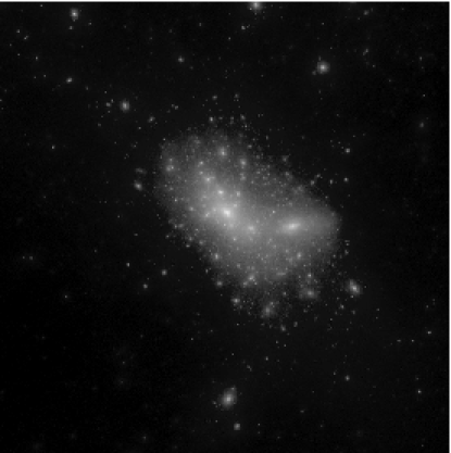
Figure 1: The structure of a dark halo at $z=0$ in $N$-body simulation based on the CDM model, using 30 million particles. This Figure is taken from Fukushige, Kawai, & Makino (2004).

It was only a decade ago that we began to be able to compute structures of dark halos in detail, because in $N$-body simulations we need numerous number of particles to achieve sufficient mass and force resolutions. However, even if we come to know structures of dark halos in theory, it’s no picnic to observe structures of dark halos. It is difficult because dark matter is dark, i.e., cannot be observed by normal methods. Thus, sometimes we have to resort to indirect methods based on several assumptions, which often turn out to be wrong or inaccurate.

2 The Crisis?

The CDM model predicts centrally concentrated mass distribution of dark halos. Navarro, Frenk, & White (1995, 1996, 1997) found in their $N$-body simulations that the spherically averaged density profiles of dark halos are well fitted by the following form:

$$\rho(r)=\frac{\rho_{\rm crit}(z)\delta_{\rm c}(z)}{\left(r/r_{\rm s}\right)\left(1+r/r_{\rm s}\right)^{2}},$$ (1)

where $\delta_{\rm c}(z)$ and $r_{\rm s}$ are characteristic density contrast and the scale radius, respectively, and both depend on the mass of dark halos. However, they claimed that the functional form of equation (1) is universal, i.e., it can be applicable to dark halos of any masses (and it is independent of cosmological parameters). This density profile is sometimes called the NFW density profile. The NFW density profile has attracted many attentions, because it seems quite unnatural for dark halos to have such universal forms, and also because it is practically useful tool in making theoretical predictions based on the CDM model. In practice, most higher-resolution $N$-body simulations indicate steeper inner profiles $\rho\sim r^{-\alpha}$ where $1\lesssim\alpha\lesssim 1.5$ (Fukushige & Makino 1997, 2001, 2003; Moore et al. 1999b; Ghigna et al. 2000; Jing & Suto 2000a; Klypin et al. 2001; Power et al. 2003; Fukushige, Kawai, & Makino 2004; Hayashi et al. 2004; Navarro et al. 2004). In any case, all $N$-body simulations predict the cuspy, centrally concentrated density profile of dark halos.

Another important prediction of the CDM model is many substructures in dark halos (see Figure 1). In the CDM model, substructures contribute 10%-15% of the total mass of the host halos (e.g., Tormen, Diaferio, & Syer 1998); thus they can affect many astrophysical/astronomical phenomena in several ways. In addition, it turned out that the substructure mass function depends on the mass of the host halo only weakly, once the mass of substructures is normalized by the mass of their host halo (e.g., Moore et al. 1999a).

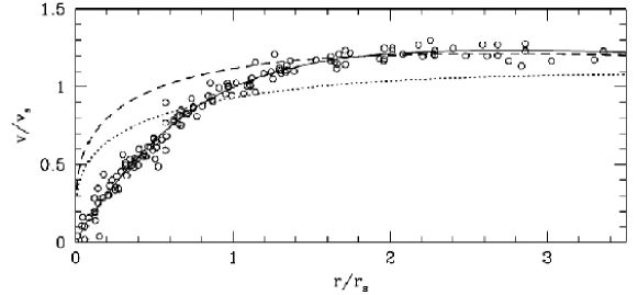
Figure 2: The rotation curves of galaxies, scaled to fit the universal density profile. The solid line indicates the rotation curve that results from the density profile with a constant density core. Dashed and dotted curves are those predicted by the $N$-body simulations.This Figure is taken from Moore et al. (1999b).

Figure 3: Abundances of substructures within the Milky Way and the Virgo Cluster are compared with those in $N$-body simulations. The cumulative numbers of substructures are plotted as a function of their circular velocity. The dotted line shows the observed distribution within the Milky Way, while open circles plot the data for the Virgo Cluster. This Figure is taken from Moore et al. (1999a).

Are the properties of dark halos consistent with observations? The answer may be no; many possible problems have been raised in both galaxy- and cluster-mass scales.

The central concentrations of dark halos have been tested using the dwarf/Low Surface Brightness (LSB) galaxy systems, mainly because in such systems dark matter dominate even near the center and the effects of baryons are thought to be small. Specifically, the rotation curves at the inner part of dwarf galaxies have been measured, and have been compared with CDM predictions. Surprisingly, it has been claimed that the cuspy profile found in $N$-body simulations cannot explain the slow rises of the rotation curves in observations. For instance, Moore et al. (1999b) explicitly showed that the universal density profile failed to reproduce observed rotation curves of dwarf/LSB galaxies (Figure 2). They claimed that the density profile with a nearly flat core is needed to fit the data.

Another problem in galaxy-mass scale is that substructures are not so common as the CDM model predicts. Moore et al. (1999a) compared abundances of substructures within the Milky Way and the Virgo Cluster with those in $N$-body simulations (Figure 3). They showed that the CDM model clearly over-predicts the number of substructures in the Milky Way, but it is consistent in the Virgo Cluster.

Figure 4: Reconstructed mass density and light density of the lensing cluster CL0024+1654 at $z=0.39$. Total (thick) and galaxy-only (thin) components of the mass are shown. Total mass profile is quite different from the one NFW predicted (dotted). This Figure is taken from Tyson et al. (1998).

In addition, there might be difficulties in the cluster-mass scale as well as in the galaxy-mass scale. Tyson, Kochanski, & Dell’Antonio (1998) reconstructed the mass distribution from the strong/weak gravitational lensing seen in the cluster CL0024+1654, and concluded that the mass distribution differs from the NFW density profile. The reconstructed mass distribution also has a nearly flat core in the mass center, as in the case of dwarf/LSB galaxies.

These results suggest that the CDM model might be wrong on small scales. A number of solutions to this problem has been proposed, including the modification of the nature of dark matter (see Appendix 10). For instance, Spergel & Steinhardt (2000) proposed interactions between dark matter particles. They showed that the elastic cross section of $\sigma_{XX}/m_{X}\sim 10^{-24}{\rm cm^{2}GeV^{-1}}$ is needed to solve the discrepancy. This, in turn, implies that detailed comparison of structures of dark halos can constrain the nature of dark matter. In the next sections, we will see the current status of the comparison to check how significant the claimed discrepancy is.

2 Testing the CDM Paradigm: Halo Concentration

1 Rotation Curves

Rotation curves in dwarf/LSB galaxies are one of the most popular methods to test the halo concentration. Many observations followed the claim of Moore et al. (1999b); de Blok et al. (2001) and de Blok & Bosma (2002) found core-dominated structures of LSB galaxies using H$\alpha$/H 1 rotation curves, and claimed that they are clearly inconsistent with the CDM model. de Blok, Bosma, & McGaugh (2003) showed that systematic effects, such as non-circular motion and off-center, are not so significant as to change the conclusions. Simon et al. (2003) reached the similar conclusion from high-resolution measurements of the dwarf spiral galaxy with H$\alpha$/CO. On the other hand, van den Bosch & Swaters (2001) and Swaters et al. (2003) also analyzed H$\alpha$ rotation curves and claimed that the current data poorly constrain the inner density profile, and that it is difficult to discriminate between cusp and core. See Figure 5 for the summary of rotation curve measurements.

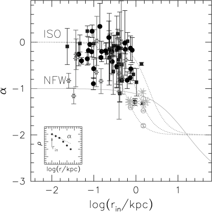
Figure 5: Inner mass density versus resolution $r_{\rm in}$ of LSB rotation curves. Unlike the text, $\alpha$ is defined by the local slope of the density profile, $\alpha=d\ln\rho/d\ln r$. Filled circles and squares show the results of de Blok et al. (2001) and de Blok & Bosma (2002), respectively. Open starts denote the results of Swaters et al. (2003). The large asterisks near $\alpha\sim-1$ and $r_{\rm in}\sim 1$kpc are the simulations by Hayashi et al. (2004). This Figure is taken from de Blok (2004).

Therefore, current observations seem to favor core rather than cusp, although the arguments against core interpretations still remain. Actually, Hayashi et al. (2004) pointed out that the discrepancy might simply reflect the difference between circular velocity and gas rotation speed. If this is true, rotation curves cannot be a good test of the halo concentration. Moreover, it might be possible that a disk bar, which should be ubiquitous in forming galaxies, produces cores in cuspy CDM halos (Weinberg & Katz 2002). Thus we need to understand how dwarf/LSB galaxies are formed, and also to clarify the relation between gas dynamics and gravitational potential in a realistic situation, before we conclude that the CDM model is inconsistent with observations.

It also should be noted that the observations probe the central regions smaller than those current $N$-body simulations are accessible. Therefore, the discrepancy could be just due to extrapolation of results of $N$-body simulations beyond the resolution.

2 Clusters of Galaxies

First we review follow-up studies of CL0024+1654 which mass distribution was claimed to be inconsistent with the CDM model by Tyson et al. (1998). Broadhurst et al. (2000) claimed that a cuspy mass distribution also can reproduce lensed images, but Shapiro & Iliev (2000) pointed out in such a cuspy model the velocity dispersion is too large to be consistent with the observation. Czoske et al. (2002) suggested that the flat density core might be produced by the high-speed collision along the line of sight which are inferred from the spectroscopy of $\sim 300$ galaxies in the cluster. However, X-ray data showed that the gas in the cluster seems to be in equilibrium (Ota et al. 2004). The lesson to be drawn from these studies, therefore, is that individual modeling of specific cluster is difficult and may suffer from the special selection function.

Besides CL0024+1654, there has been many attempts to constrain the halo concentration with lensing clusters. Smith et al. (2001) found steep inner profile ($\alpha\sim 1.3$) in A383. Gavazzi et al. (2003) analyzed MS2137$-$2353 and found that cored profile better reproduce the lensed images. Weak lensing analyses have been also done in several clusters. Basically they are consistent with the NFW density profile (Clowe & Schneider 2001, 2002; Dahle, Hannestad, & Sommer-Larsen 2003), although the cored profile tends to fit the data equally.

Figure 6: PDFs of the inner density profile ($\beta$ should be read $\alpha$). Left: PDFs for radial arc clusters. Right: PDFs for tangential arc clusters. These Figures are taken from Sand et al. (2004).

Recently, Sand et al. (2004) studied 6 lensing clusters in detail, and claimed that they are inconsistent with the CDM model on average (see Figure 6). They showed that clusters with radial arcs are well constrained to $\alpha\sim 0.5$, though scatter is very large, and that clusters with only tangential arcs give upper limit on the inner slope, $\alpha\lesssim 0.5$. Both tangential and radial arc clusters strongly disfavor the NFW density profile. However, the result strongly relies on several simplified assumptions, such as the spherical symmetry and the fixed value of the scale radius; Bartelmann & Meneghetti (2004) and Dalal & Keeton (2004b) showed that steep inner density profiles can be reconciled with the data if we relax the assumptions. Their arguments clearly demonstrate that the degeneracy between mass distributions is so significant that it is quite difficult to draw conclusions from the modeling of lensing clusters only.

An additional constraint comes from X-ray observations, by assuming hydrostastic equilibrium. Tamura et al. (2000) found that ASCA and ROSAT measurements of the cluster A1060 are consistent with the NFW density profile. Lewis et al. (2003) and Buote & Lewis (2004) measured X-ray luminosity and temperature profiles of regular, relaxed clusters A2029 and A2589, and found that the density profiles show good agreements with the CDM predictions. Specifically, the inner slope is constrained to $\alpha=1.19\pm 0.04$ for A2029 and to $\alpha=1.35\pm 0.21$ for A2589, respectively. It seems like that X-ray data basically support for the CDM model, but analyses in more clusters will be important to draw a robust conclusion.

3 Testing the CDM Paradigm: Halo Shape

Shapes of dark halos also give us insight on the nature of dark matter. In the CDM model, dark halos are not spherical, but rather triaxial (e.g., Jing & Suto 2002). Collisions between dark matter particles always make dark halos rounder, thus observations of elongated triaxial dark halos would support for the CDM model. Indeed, Yoshida et al. (2000a, b) found in their series of $N$-body simulations that self-interactions of dark matter do make the core of dark halos rounder. Figure 7 clearly demonstrate how collisions affect the shape of dark halos.

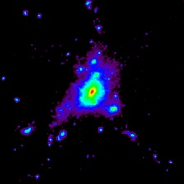
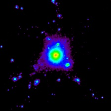
Figure 7: Dark matter distributions in simulated clusters. Left: The shape of dark halos in the standard CDM model. Right: The shape of dark halos in the weakly self-interacting dark matter model with the cross section of $\sigma_{XX}=10{\rm cm^{2}}g^{-1}$. This Figure is taken from Yoshida et al. (2000b).

Observations seem inconsistent with this round halo; Buote et al. (2002) observed the elliptical galaxies NGC720 with X-ray, and found that the axis ratio of $\sim 0.4$ gives the best fit to the data; Miralda-Escudé (2002) analyzed the lensing cluster MS2137$-$2353 and discussed that the projected ellipticity of $\gtrsim 0.2$ is required to fit the lensed images; Hoekstra, Yee, & Gladders (2004) derived the average ellipticity of dark halos from weak lensing as $\langle e\rangle=0.33^{+0.07}_{-0.09}$. These results suggest that collisions are not so significant as to modify the shape of dark halos. However, it should be noted that axis ratios have quite broad probability distribution in the CDM model (Jing & Suto 2002), and this might be also the case for self-interacting dark matter model. If so, we need large number of dark halos to test the shapes so as not to be affected by sample variance.

4 Testing the CDM Paradigm: Halo Substructures

1 Satellite Galaxies

The over-abundance of substructures in galactic halos, as shown in Figure 3, has raised many discussions. The abundant substructures are firm prediction of the CDM model, because many independent numerical simulations have confirmed the fact that the CDM model predicts roughly 10%-15% of mass in a dark halo is bound to substructures (Tormen et al. 1998; Klypin et al. 1999; Okamoto & Habe 1999; Ghigna et al. 2000; Springel et al. 2001; Zentner & Bullock 2003; De Lucia et al. 2004; Kravtsov, Gnedin, & Klypin 2004). The fraction of substructures is also supported by theory (e.g., Oguri & Lee 2004d). Popular ways to resolve the conflict include modifying the nature of dark matter (see Appendix 10) and introducing new inflationary models that can produce density fluctuations with small-scale power cut-off such as an inflation model with broken scale-invariance (Kamionkowski & Liddle 2000) and a double hybrid inflation (Yokoyama 2000).

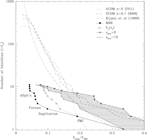
Figure 8: Abundance of substructures within the Milky Way are compared with those in $N$-body simulations (see also Figure 3). Numerical simulations of Font et al. (2001), Moore et al. (1999a), and Klypin et al. (1999) are plotted to show the robustness of simulation results. Filled circles show the observed distribution assuming the isothermal potential as in Moore et al. (1999a). Open circles plot circular velocities at luminosity cutoff assuming the NFW density profile. In the shaded region, observed velocities are converted to peak velocities of unstripped NFW halos (the uncertainty reflects different accretion time). Now there is no major discrepancy for massive substructures, $V_{\rm max}/V_{200}\gtrsim 0.16$. This Figure is taken from Hayashi et al. (2003).

However, the problem may be resolved also by taking account of astrophysical processes such as photo-ionizing background (Somerville 2002) and inefficient star formation in small mass halos (Stoehr et al. 2002). These ideas claim that the observed number of satellite galaxies is small because only very massive substructures contain stars and most substructures are dark. These ideas based on the dark substructures, however, may not be consistent with observations, either: Recent high-resolution numerical simulations have found that the massive substructures tend to place in the outer part of host halos, which is not the case for the satellites of the Milky Way (e.g., De Lucia et al. 2004).

On the other hand, Hayashi et al. (2003) claimed that the apparent discrepancy of abundances of massive substructures is caused by the large difference between tidal radii of substructures in simulations and radial cutoff observed in surface brightness profiles. This implies that it may be possible to account for observed abundance of substructures without invoking the nature of dark matter and/or photo-ionizing background. Figure 8 illustrates the result. This result suggests that we must be careful in comparing abundances of satellite galaxies with $N$-body simulations. Even in their results, low-mass substructures shows the difference, and this may be caused by complicated astrophysical processes, such as the efficient feedback and evaporation of gas.

2 Gravitational Lensing

As suggested in the previous subsection, one of main difficulties in the comparison between simulations and observation is that substantial fraction of substructures may be dark. It is quite hard to test the existence of such dark substructures observationally.

Gravitational lensing can avoid such problem; it can detect substructures directly even if they are dark. The existence of substructures in lensed quasar systems was first suggested by Mao & Schneider (1998). They claimed that the anomalous flux ratio in the quadruple lens B1422+231 is due to substructures in the lens galaxy. Indeed, it has been shown that the large amount of substructures predicted in the CDM model is needed to account for flux anomalies in several lens systems (Metcalf & Zhao 2002; Chiba 2002; Dalal & Kochanek 2002; Bradač et al. 2002; Kochanek & Dalal 2004a). As an example, Figure 9 shows how much the CDM substructures can change the flux ratios between multiple images. Although the observed flux ratios are very different from the median flux ratios predicted in modeling, the probability distributions of flux ratios induced by the CDM substructures are so broad that the anomalous flux ratios can be reconciled with the mass modeling.

Figure 9: Upper: Image configurations of lensed quasar systems B1422+231 and PG1115+080. Lower: Probability distributions of images in the lensed quasar systems. As models of substructures, globular clusters (GL), dwarf satellites (DW), and CDM substructures (CDM) are considered. Fluxes are normalized by those of image B (B1422+231) and image A1 (PG1115+080). The flux ratio $r$ for B1422+23 is defined by $r=(A+B+C)/(|A|+|B|+|C|)$. Observed flux ratios are denoted by short vertical bars. These Figures are taken from Chiba (2002).

Caveats about this method are that the results are sensitive to the spatial distribution of substructures (Chen, Kravtsov, & Keeton 2003), and that there is a degeneracy with the complexity of the smooth components (Evans & Witt 2003; Keeton, Gaudi, & Petters 2003c; Kochanek & Dalal 2004a; Kawano et al. 2004). Actually, substructures we need to fit flux rations might be even larger than the CDM model predicts, when we take account of the spatial distribution (Evans & Witt 2003; Mao et al. 2004). Therefore these flux anomalies might be caused by stellar components in the lens galaxies (Schechter & Wambsganss 2002) or massive black holes ($\sim 10^{5}-10^{6}M_{\odot}$) in the halos (Mao et al. 2004), rather than the CDM substructures. To avoid these problems, it may be needed to develop more sophisticated methods, such as spectroscopic lensing (e.g., Metcalf et al, 2004) and mesolensing, i.e., additional strong lensing of multiple images by substructures (Yonehara, Umemura, & Susa 2003).

5 Need for More Studies

We have reviewed various tests of the CDM paradigm at small non-linear scales. Although the situation is not so bad as first insisted (§2), it is still inconclusive whether these observations are well explained by the CDM model or not. In particular, a confusion comes from the fact that similar approaches sometimes yield different conclusions. This implies that systematic effects, e.g., the selection effect, the treatment of astrophysical processes, degeneracy with other parameters, etc., are very important. The understanding of astrophysical processes is especially important in using indirect methods such as rotation curves of galaxies.

In conclusion, we need more studies; we need more independent tests in order to come to a firm conclusion on the validity of the CDM model on small scales, as well as the improvements of each test. Think of the reason why the concordance model (Chapter 1) is now accepted widely; this is because many independent tests point to the concordance model! We believe results on small scales also converge to somewhere as we add more observations, though no one knows where it is.

Chapter 3 Gravitational Lensing by Triaxial Dark Halos

1 Why Do We Need Non-Spherical Lens Models?

In this thesis, we newly construct a non-spherical lens model for lens statistics (see Appendix 11 for basics of gravitational lensing). Actually, there has been no work on cluster-scale lens statistics that adopts non-spherical lens models (see Introductions of Chapters 4 and 5), despite CDM halos are not spherical at all (see Chapter 2). The main reasons are (1) non-spherical modeling makes it much more difficult to compute lensing cross sections and hence lens statistics, and (2) we didn’t have a reliable model of non-spherical descriptions of lens objects, i.e., dark halos. As for (2), however, it is now possible to construct such non-spherical model using high-resolution $N$-body simulations. For instance, Jing & Suto (2002) fitted dark halos by the triaxial model and derived the probability distribution functions (PDFs) of the triaxiality from their cosmological simulations. These modelings enable us to incorporate the non-sphericity in the lens statistics. To overcome (1), we will develop semi-analytic methods to compute the number of lenses in triaxial dark matter halos in Chapters 4 and 5. This combines the lensing cross section from the Monte Carlo ray-tracing simulations and the probability distribution function of the axis ratios evaluated from the cosmological simulations.

However, why do we need non-spherical lens models in statistical studies? One of the most important reasons is that the deviation from the spherical symmetry affects gravitational lensing drastically. We illustrate this in Figure 1. In the spherical mass distribution, there is only one caustic curve (radial caustic), because the tangential caustic degenerates at the center of mass distribution. But, once we introduce non-sphericity in the mass distribution, the tangential caustic no longer degenerates; it grows as increasing the ellipticity, and at last it becomes much larger than the radial caustic. Since the probability for multiple images is proportional to the strong lensing cross section which is given by the area enclosed by caustics, it is expected that the non-sphericity has a great impact on lens statistics.

Another important reason that we need to include the non-sphericity is image multiplicities. Since it is shown that the number of images increases (or decreases) by 2 when the source crosses a caustic, spherical halos can produce 3 images at most. This is not the case for non-spherical halos; the elliptical halos shown in Figure 1 can produce more than 3 images due to non-degenerate tangential caustics. In addition, the topology of caustics is sensitive to the degree of the non-sphericity, as seen in Figure 1. In the observational side, many lensed quasar systems with more than 3 images have been discovered so far. Thus the non-spherical modeling conveys us qualitatively new information on mass distributions of lens objects.

In short, the non-spherical lens modeling is an essential ingredient for lens statistics, rather than a minor upgrade; it can change lens probabilities drastically, and it offers us new information on the shape of clusters.

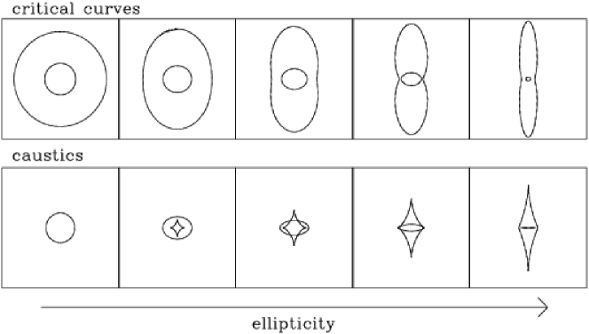
Figure 1: Illustration on how critical curves (upper) and caustics (lower) changes as the ellipticity of the projected mass density distribution is increased (from $e=0$ to $e=0.8$). In this plot, we adopt the elliptical NFW density profile. The first column shows those of the spherical mass distribution.

2 Description of Triaxial Dark Matter Halos

In this section, we briefly summarize the triaxial model of dark matter halos proposed by Jing & Suto (2002, referred as JS02 in the rest of this chapter). They obtained the detailed triaxial modeling on the basis of their high-resolution individual halo simulations as well as large-scale cosmological simulations. Most importantly, they provided a series of useful fitting formulae for mass- and redshift-dependence and the PDFs of the axis ratio and the concentration parameter. Such detailed and quantitative modeling enables us to incorporate the non-sphericity of dark matter halos in a reliable manner.

1 Isodensity Surfaces

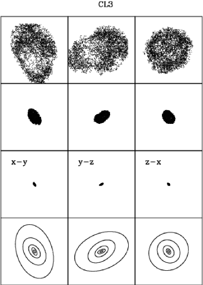
Figure 2: Examples of projected particles distributions in a cluster-size halo. From top to bottom, particles in the isodensity shells with $A=100$, $2500$, $6.25\times 10^{4}$ are plotted. The bottom panels show triaxial fits to five isodensity surfaces defined in equation (5). This Figure is taken from JS02.

JS02 adopted the following method to find isodensity surfaces. First they begin with the computation of a local density at each particle’s position by using the smoothing kernel (e.g., Hernquist & Katz 1989):

$$W(r,h_{i})=\frac{1}{\pi h_{i}^{3}}\left\{\begin{array}[]{ll}{\displaystyle 1-\frac{3}{2}\left(\frac{r}{h_{i}}\right)^{2}+\frac{3}{4}\left(\frac{r}{h_{i}}\right)^{3}}&\mbox{($r\leq h_{i}$)}\\ {\displaystyle\frac{1}{4}\left(2-\frac{r}{h_{i}}\right)^{3}}&\mbox{($h_{i}<r<2h_{i}$)}\\ {\displaystyle 0}&\mbox{otherwise,}\end{array}\right.$$ (4)

with $h_{i}$ being the smoothing length for $i$-th particle. They use 32 nearest neighbor particles to compute the local density $\rho_{i}$. The smoothing length $h_{i}$ is set to be one-half the radius of the sphere that contains those 32 neighbors. Then, from $\rho_{i}$ they construct the isodensity surfaces corresponding to the five different thresholds:

$$\rho_{s}^{(n)}=A^{(n)}\rho_{\rm crit},\;\;\;\;\;A^{(n)}=100\times 5^{n-1}\;\;(n=1\sim 5).$$ (5)

Actually they collected all particles with $0.97\rho_{s}^{(n)}<\rho_{i}<1.03\rho_{s}^{(n)}$ and determined $n$-th isodensity surface. To obtain the isodensity surfaces of the overall density profile, they eliminate small distinct regions caused by the substructures.

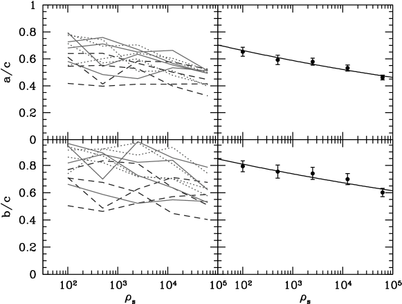
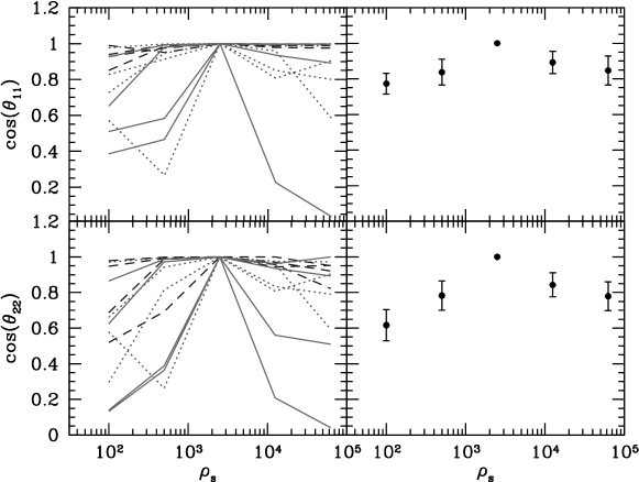
Figure 3: Axis ratios (top) and degree of alignments (bottom) on $\rho_{s}$, from fits to 12 halos. Right panels show the mean and its $1\sigma$ error. The angle $\theta_{11}$ is defined by the angle between major axis of the isodensity surface and that of the $A^{(3)}=2500$ isodensity surface. Similarly, $\theta_{22}$ is defined with respect to the middle axes. These Figures are taken from JS02.

An example is shown in Figure 2. Since the isodensity surfaces are well approximated by triaxial ellipsoids, JS02 fitted the isodensity surfaces by the following form:

$$R^{2}(\rho_{s})=\frac{X^{2}}{a^{2}(\rho_{s})}+\frac{Y^{2}}{b^{2}(\rho_{s})}+\frac{Z^{2}}{c^{2}(\rho_{s})},$$ (6)

where the lengths of principal vectors are chosen as $a\leq b\leq c$. The dependence of axis ratios and the degree of alignments on $\rho_{s}$ is summarized in Figure 3. Axis ratios weakly depend on $\rho_{s}$; the isodensity surfaces become more elongated in the central region than in the outer region. It is also found that the alignments are basically good; $\cos\theta_{11}\gtrsim 0.7$ and $\cos\theta_{22}\gtrsim 0.6$. These agreement makes sense to approximate a dark halo as the triaxial ellipsoid with the same axis ratios and axis directions for the entire halo. Thus JS02 measured axis ratios from the isodensity surface for $A^{(3)}=2500$, and regards them as the axis ratios of the whole dark halo.

2 Density Profile of Triaxial Dark Matter Halos

By considering triaxial shells in the way discussed in the previous subsection, JS02 found that the following density profiles of triaxial dark halos fit quite well:

$$\rho(R)=\frac{\delta_{\rm ce}\rho_{\rm crit}(z)}{(R/R_{0})^{\alpha}(1+R/R_{0})^{3-\alpha}},$$ (7)

where

$$R^{2}\equiv c^{2}\left(\frac{x^{2}}{a^{2}}+\frac{y^{2}}{b^{2}}+\frac{z^{2}}{c^{2}}\right)\;\;\;(a\leq b\leq c).$$ (8)

The precise value of the inner slope, $\alpha$, is still controversial, but almost all the N-body simulations based on the collisionless CDM scenario indicate values between $1$ and $1.5$ (Navarro et al. 1996, 1997; Fukushige & Makino 1997, 2001, 2003; Moore et al. 1999b; Ghigna et al. 2000; Jing & Suto 2000a; Klypin et al. 2001; Power et al. 2003; Fukushige et al. 2004; Hayashi et al. 2004; Navarro et al. 2004). Thus in this thesis we consider both $\alpha=1$ and $\alpha=1.5$ so as to cover a possible range of the CDM predictions.

JS02 defined the concentration parameter in the triaxial model as

$$c_{e}\equiv\frac{R_{e}}{R_{0}},$$ (9)

where $R_{e}$ is chosen so that the mean density within the ellipsoid of the major axis radius $R_{e}$ is $\Delta_{e}\Omega_{M}(z)\rho_{\rm crit}(z)$ with

$$\Delta_{e}=5\Delta_{\rm vir}\left(\frac{c^{2}}{ab}\right)^{0.75}.$$ (10)

Here $\Omega_{M}(z)$ and $\rho_{\rm crit}(z)$ denote the matter density parameter and the critical density of universe at redshift $z$, respectively, and $\Delta_{\rm vir}(z)$ denotes the overdensity of objects virialized at $z$ (see §8.D).

Then the characteristic density $\delta_{\rm ce}$ in equation (7) is written in terms of the concentration parameter $c_{e}$ as

$$\delta_{\rm ce}=\frac{\Delta_{e}\Omega_{M}(z)}{3}\frac{c_{e}^{3}}{m(c_{e})},$$ (11)

where $m(c_{e})$ is

$$m(c_{e})\equiv\frac{c_{e}^{3-\alpha}}{3-\alpha}\,{}_{2}F_{1}\left(3-\alpha,3-\alpha;4-\alpha;-c_{e}\right),$$ (12)

with ${}_{2}F_{1}\left(a,b;c;x\right)$ being the hypergeometric function. For $\alpha=1$ and $1.5$, equation (12) simply reduces to

$$m(c_{e})=\left\{\begin{array}[]{ll}\displaystyle{\ln(1+c_{e})-\frac{c_{e}}{1+c_{e}}}&\mbox{($\alpha=1$)},\\ \displaystyle{2\ln(\sqrt{c_{e}}+\sqrt{1+c_{e}})-2\sqrt{\frac{c_{e}}{1+c_{e}}}}&\mbox{($\alpha=1.5$)}.\end{array}\right.$$ (15)

Since $R_{e}$ is empirically related to the (spherical) virial radius $r_{\rm vir}$ as $R_{e}/r_{\rm vir}\simeq 0.45$ (JS02), the scaling radius in the triaxial model, $R_{0}$, for a halo of a mass $M_{\rm vir}$ is given as

$$R_{0}=0.45\frac{r_{\rm vir}}{c_{e}}=\frac{0.45}{c_{e}}\left(\frac{3M_{\rm vir}}{4\pi\Delta_{\rm vir}\Omega_{M}(z)\rho_{\rm crit}(z)}\right)^{1/3}.$$ (16)

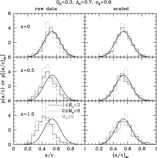
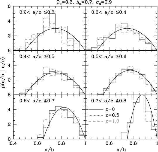
Figure 4: Distributions of axis ratios, $a/c$ (top) and $a/b$ (bottom). Different lines denote different number of particles (i.e., mass). Specifically, the number of particles within virial radius is described by $M_{4}\equiv(N_{\rm halo}/10^{4})$. The scaled axis ratio $(a/c)_{\rm sc}$ is defined by equation (19). Lines show fits to data (eqs. [17] and [18]). These Figures are taken from JS02.

Since we do not know the properties of the density profile of an individual lensing halo, our prediction for lensing probabilities is necessarily statistical in a sense that it should be made after averaging over appropriate PDFs of the properties of halos. For this purpose, we need the PDFs of axis ratios. JS02 empirically derived such PDFs from their cosmological simulations. For the axis ratios, they are given as

$$p(a/c)=\frac{1}{\sqrt{2\pi}\times 0.113}\exp\left[-\frac{\left\{(a/c)_{\rm sc}-0.54\right\}^{2}}{2(0.113)^{2}}\right]\frac{(a/c)_{\rm sc}}{a/c},$$ (17)

and

$$p(a/b|a/c)=\frac{3}{2(1-\max(a/c,0.5))}\left[1-\left(\frac{2a/b-1-\max(a/c,0.5)}{1-\max(a/c,0.5)}\right)^{2}\right],$$ (18)

for $a/b\geq\max(a/c,0.5)$, and $p(a/b|a/c)=0$ otherwise (JS02). Here $M_{*}$ is the characteristic nonlinear mass so that the rms top-hat smoothed overdensity at that mass scale is $1.68$. The scaled axis ratio $(a/c)_{\rm sc}$ is defined by

$$\left(\frac{a}{c}\right)_{\rm sc}\equiv\left(\frac{a}{c}\right)\left(\frac{M_{\rm vir}}{M_{*}}\right)^{0.07[\Omega_{M}(z)]^{0.7}},$$ (19)

and represents the mass and redshift dependences of axis ratios. In Figure 4, we show how well these fitting formulae work. For the concentration parameter,

$$p(c_{e})=\frac{1}{\sqrt{2\pi}\times 0.3}\exp\left[-\frac{(\ln c_{e}-\ln\bar{c}_{e})^{2}}{2(0.3)^{2}}\right]\frac{1}{c_{e}},$$ (20)

where the fit to the median concentration parameter $\bar{c}_{e}$ for $\alpha=1$ is given as :

$$\bar{c}_{e}=1.35\exp\left[-\left\{\frac{0.3}{(a/c)_{\rm sc}}\right\}^{2}\right]A_{e}\sqrt{\frac{\Delta_{\rm vir}(z_{c})}{\Delta_{\rm vir}(z)}}\left(\frac{1+z_{c}}{1+z}\right)^{3/2},$$ (21)

with $z_{c}$ being the collapse redshift of the halo of mass $M_{\rm vir}$ (JS02). In the case of $\alpha=1$, we simply use the above expression, and for $\alpha=1.5$, we use the relation $\bar{c}_{e}(\alpha=1.5)=0.5\bar{c}_{e}(\alpha=1)$ (Keeton & Madau 2001a; JS02). JS02 estimated $A_{e}=1.1$ in the Lambda-dominated CDM model, but this value is likely to be dependent on the underlying cosmology to some extent. As we stressed in Chapter 1, however, we fix cosmological parameters to those of the “concordance” cosmology. Therefore in this thesis we mostly fix the value to $A_{e}=1.1$.

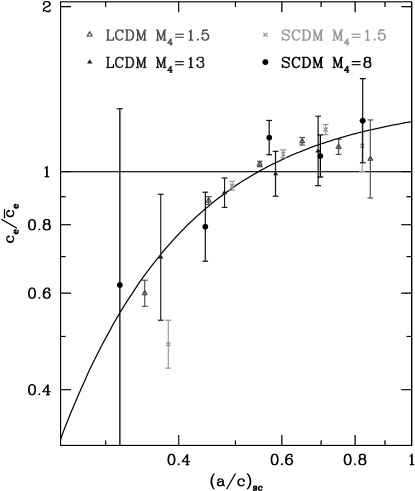
Figure 5: Dependence of the concentration parameter $c_{e}$ on the axis ratio. The fitting formula (prefactor in equation [21]) is also shown by the solid line. This Figure is taken from JS02.

3 Lensing Properties of Triaxial Dark Matter Halos

In this section, we present several expressions for triaxial dark matter halos which are useful in calculating gravitational lensing properties. Under the thin lens approximation, gravitational lensing properties are fully characterized by the matter density projected along the line-of-sight (see Appendix 11). We have to calculate the mass density profile projected along the arbitrary line-of-sight directions, because the line-of-sight, in general, does not coincide with the principal axis of a triaxial dark matter halo.

1 Coordinate Systems

We introduce two Cartesian coordinate systems, $\vec{x}=(x,y,z)$ and $\vec{x^{\prime}}=(x^{\prime},y^{\prime},z^{\prime})$, which represent respectively the principal coordinate system of the triaxial dark halo and the observer’s coordinate system. The origins of both coordinate systems are set at the center of the halo. It is assumed that the $z^{\prime}$-axis runs along the line-of-sight direction of the observer, and that the $z$-axis lies along the major principal axis. In general, the relative orientation between the two coordinate systems can be specified by the three Euler angles. However, in our case, it is only the line-of-sight direction that is fixed while the rotation angle of the $x^{\prime}$-$y^{\prime}$ plane relative to $x$-$y$ plane is arbitrary, and thus we may need only two angles to specify the relative orientation of the two coordinate systems. Here we make a choice of $x^{\prime}$-axis lying in the $x$-$y$ plane. Then the relative orientation of the two coordinate systems can be expressed in terms of the line-of-sight direction in the halo principal coordinate system.

Let $(\theta,\phi)$ be the polar coordinates of the line-of-sight direction in the $\vec{x}$-coordinate system. Then the relation between the two coordinate systems can be expressed in terms of the rotation matrix $A$ (Binney 1985) as

$$\vec{x}=A\vec{x^{\prime}},$$ (22)

where

$$A\equiv\left(\begin{array}[]{ccc}-\sin\phi&-\cos\phi\cos\theta&\cos\phi\sin\theta\\ \cos\phi&-\sin\phi\cos\theta&\sin\phi\sin\theta\\ 0&\sin\theta&\cos\theta\\ \end{array}\right).$$ (23)

Figure 6 represents the relative orientation between the observer’s coordinate system and the halo principal coordinate system.

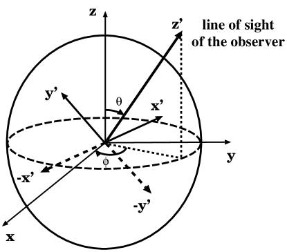
Figure 6: The orientations of the coordinate systems. The Cartesian axes ($x,y,z$) represent the halo principal coordinate system while the axes ($x^{\prime},y^{\prime},z^{\prime}$) stand for the observers coordinate system with $z^{\prime}$-axis aligned with the line-of-sight direction. The $x^{\prime}$-axis lies in the $x$-$y$ plane. The angle $(\theta,\phi)$ represent the polar angle of the line-of-sight direction in the $(x,y,z)$-coordinate system.

2 Lensing Properties

For simplicity, in this section we redefine $\vec{x}/R_{0}$ and $\vec{x^{\prime}}/R_{0}$ as $\vec{x}$ and $\vec{x^{\prime}}$, respectively. In this case,

$$\rho(R)=\frac{\delta_{\rm ce}\rho_{\rm crit}(z)}{R^{\alpha}(1+R)^{3-\alpha}},$$ (24)

with $R$ being defined by equation (8). In terms of the observer’s coordinates $(x^{\prime},y^{\prime},z^{\prime})$, $R$ is written as

$$R=\sqrt{fz^{\prime 2}+gz^{\prime}+h},$$ (25)

where

$$f = \sin^{2}\theta\left(\frac{c^{2}}{a^{2}}\cos^{2}\phi+\frac{c^{2}}{b^{2}}\sin^{2}\phi\right)+\cos^{2}\theta,$$ (26)

$$g = \sin\theta\sin 2\phi\left(\frac{c^{2}}{b^{2}}-\frac{c^{2}}{a^{2}}\right)x^{\prime}+\sin 2\theta\left(1-\frac{c^{2}}{a^{2}}\cos^{2}\phi-\frac{c^{2}}{b^{2}}\sin^{2}\phi\right)y^{\prime},$$ (27)

$$h = \left(\frac{c^{2}}{a^{2}}\sin^{2}\phi+\frac{c^{2}}{b^{2}}\cos^{2}\phi\right)x^{\prime 2}+\sin 2\phi\cos\theta\left(\frac{c^{2}}{a^{2}}-\frac{c^{2}}{b^{2}}\right)x^{\prime}y^{\prime}$$ (28)

$$+\left[\cos^{2}\theta\left(\frac{c^{2}}{a^{2}}\cos^{2}\phi+\frac{c^{2}}{b^{2}}\sin^{2}\phi\right)+\sin^{2}\theta\right]y^{\prime 2}.$$

Defining two new variables $z^{\prime}_{*}$ and $\zeta$

$$z^{\prime}_{*}{} \equiv \sqrt{f}\left(z^{\prime}+\frac{g}{2f}\right),$$ (29)

$$\zeta \equiv h-\frac{g^{2}}{4f},$$ (30)

we rewrite equation (25) as

$$R=\sqrt{z^{\prime}_{*}{}^{2}+\zeta^{2}}.$$ (31)

Then the convergence $\kappa$ can be expressed as a function of $\zeta$:

$$\kappa=\frac{R_{0}}{\Sigma_{\rm crit}}\int_{-\infty}^{\infty}\rho(R)dz^{\prime}=\frac{R_{0}}{\Sigma_{\rm crit}}\int_{-\infty}^{\infty}\frac{1}{\sqrt{f}}\rho\left(\sqrt{z^{\prime}_{*}{}^{2}+\zeta^{2}}\right)dz^{\prime}_{*}\equiv\frac{b_{\rm TNFW}}{2}f_{\rm GNFW}(\zeta),$$ (32)

where

$$b_{\rm TNFW}\equiv\frac{1}{\sqrt{f}}\frac{4\delta_{\rm ce}\rho_{\rm crit}(z)R_{0}}{\Sigma_{\rm crit}},$$ (33)

and

$$f_{\rm GNFW}(r)\equiv\int_{0}^{\infty}\frac{1}{\left(\sqrt{r^{2}+z^{2}}\right)^{\alpha}\left(1+\sqrt{r^{2}+z^{2}}\right)^{3-\alpha}}dz.$$ (34)

The critical surface mass density (see Appendix 11) is denoted by $\Sigma_{\rm crit}$.

The meaning of the variable $\zeta$ can be easily understood by substituting equations (26)-(28) into equation (30):

$$\zeta^{2}=\frac{1}{f}\left(Ax^{\prime 2}+Bx^{\prime}y^{\prime}+Cy^{\prime 2}\right),$$ (35)

where

$$A \equiv \cos^{2}\theta\left(\frac{c^{2}}{a^{2}}\sin^{2}\phi+\frac{c^{2}}{b^{2}}\cos^{2}\phi\right)+\frac{c^{2}}{a^{2}}\frac{c^{2}}{b^{2}}\sin^{2}\theta,$$ (36)

$$B \equiv \cos\theta\sin 2\phi\left(\frac{c^{2}}{a^{2}}-\frac{c^{2}}{b^{2}}\right),$$ (37)

$$C \equiv \frac{c^{2}}{b^{2}}\sin^{2}\phi+\frac{c^{2}}{a^{2}}\cos^{2}\phi.$$ (38)

The quadratic form of equation (35) implies that the iso-$\zeta$ curves are ellipses, and that the position angle of ellipses $\psi$ is

$$\psi=\frac{1}{2}\arctan\frac{B}{A-C}.$$ (39)

Figure 7: PDFs of $q$ (eq. [43]), $q_{x}$ (eq. [41]), and $q_{y}$ (eq. [42]). Here we consider a halo with mass $M_{\rm vir}=10^{15}h^{-1}M_{\odot}$ and redshift $z=0.3$, but the result only weakly depends on the halo mass and redshift. These PDFs are calculated from PDFs of axis ratios $p(a/c)$ and $p(a/b)$ for which we use equations (17) and (18). We assume that the orientations of dark halos are random.

By rotating the $x^{\prime}y^{\prime}$-plane by the angle $\psi$, we diagonalize equation (35) such that

$$\zeta^{2}=\frac{x^{\prime 2}}{q_{x}^{2}}+\frac{y^{\prime 2}}{q_{y}^{2}},$$ (40)

where

$$q_{x}^{2} \equiv \frac{2f}{A+C-\sqrt{(A-C)^{2}+B^{2}}},$$ (41)

$$q_{y}^{2} \equiv \frac{2f}{A+C+\sqrt{(A-C)^{2}+B^{2}}}.$$ (42)

Note that $q_{x}\geq q_{y}$ for the given $\psi$. We further define the axis ratio $q$ as

$$q\equiv\frac{q_{y}}{q_{x}}=\left(\frac{A+C-\sqrt{(A-C)^{2}+B^{2}}}{A+C+\sqrt{(A-C)^{2}+B^{2}}}\right)^{1/2},$$ (43)

which represents the ellipticities of the projected isodensity curves of the triaxial dark halos. In this case, the convergence $\kappa$ is expressed as

$$\kappa=\kappa(\xi),\;\;\;\;\;\;\mbox{where }\xi^{2}=x^{\prime}{}^{2}+\frac{y^{\prime}{}^{2}}{q^{2}}.$$ (44)

The advantage of this diagonalization is that we can apply the previous method to calculate lensing properties (Schramm 1990; Keeton 2001d) where the deflection angle $\vec{\alpha}=(\alpha_{x^{\prime}},\alpha_{y^{\prime}})$ is expressed as a one-dimensional integral of the convergence $\kappa(\xi)$:

$$\alpha_{x^{\prime}}(x^{\prime},y^{\prime}) = qx^{\prime}J_{0}(x^{\prime},y^{\prime}),$$ (45)

$$\alpha_{y^{\prime}}(x^{\prime},y^{\prime}) = qy^{\prime}J_{1}(x^{\prime},y^{\prime}),$$ (46)

where the integral $J_{n}(x,y)$ is

$$J_{n}(x,y)=\int_{0}^{1}\frac{\kappa\left(\xi(v)\right)}{\left[1-(1-q^{2})v\right]^{n+1/2}}dv,$$ (47)

and $\xi(v)$ is

$$\xi^{2}(v)=v\left(x^{2}+\frac{y^{2}}{1-(1-q^{2})v}\right).$$ (48)

Figure 7 plots PDFs of $q$, $q_{x}$, and $q_{y}$. They were computed numerically using equations (17)-(18) and (41)-(43) under the assumption that the triaxial halo orientations (i.e., the angles $\theta$ and $\phi$) are randomly distributed. In this plot we set $M_{\rm vir}=10^{15}h^{-1}M_{\odot}$ and $z=0.3$, which are s typical mass scale and a redshift of lensing clusters. It is clear from Figure 7 that the axis ratio of projected isodensity contours strongly deviates from unity, having maximum around $q\sim 0.6$. This large degree of ellipticity suggests that the triaxial dark halos in realistic cosmological models significantly enhances lensing cross sections compared with the conventional spherical model predictions.

Figure 8: Comparison of $f_{\rm GNFW}(r)$ for $\alpha=1.5$ (denoted by “Integral”; see eq. [34]) and its fitting formula (denoted by “Fit”; see eq. [52]). “Error” plotted in the bottom panel is defined by $[f_{\rm GNFW}({\rm Integral})-f_{\rm GNFW}({\rm Fit})]/f_{\rm GNFW}({\rm Integral})$.

For $\alpha=1$, $f_{\rm GNFW}(r)$ defined in equation (34) is analytically expressed as (Bartelmann 1996):

$$f_{\rm GNFW}(r)=\left\{\begin{array}[]{ll}{\displaystyle\frac{1}{1-r^{2}}\left[-1+\frac{2}{\sqrt{1-r^{2}}}{\rm arctanh}\sqrt{\frac{1-r}{1+r}}\right]}&\mbox{($r<1$),}\\ {\displaystyle\frac{1}{r^{2}-1}\left[1-\frac{2}{\sqrt{r^{2}-1}}\arctan\sqrt{\frac{r-1}{r+1}}\right]}&\mbox{($r>1$),}\end{array}\right.$$ (51)

but it does not has a simple analytical expression for $\alpha=1.5$. Thus we use the following fitting formula in this case:

$$f_{\rm GNFW}(r)=\frac{2.614}{r^{0.5}\left(1+2.378r^{0.5833}+2.617r^{1.5}\right)}.$$ (52)

The error of the above fit is $\lesssim 0.6$% (see Figure 8).

We note that the triaxial dark halo model we presented in this section can be improved in several ways. First, we assumed that the axis ratios of the triaxial ellipsoids are constant with radius. However, JS02 showed that the axis ratios decrease slightly toward the halo centers: $a/c$ decreases by $\sim\!0.2$ as the mean radius decreases from $\sim\!0.6r_{\rm vir}$ to $\sim\!0.06r_{\rm vir}$ (see Figure 3). Since strong lensing is most sensitive to the inner parts of dark halos, it is possible that we have actually underestimated the effects of triaxiality on the statistics of large-separation lenses. On the other hand, including baryons (which were neglected in the simulations of JS02) would tend to make dark halos rounder by $\Delta(a/c)\sim 0.1$–$0.2$ (e.g., Kazantzidis et al. 2004).

4 Effect of Triaxiality on Strong Gravitational Lensing

1 Projection Effect

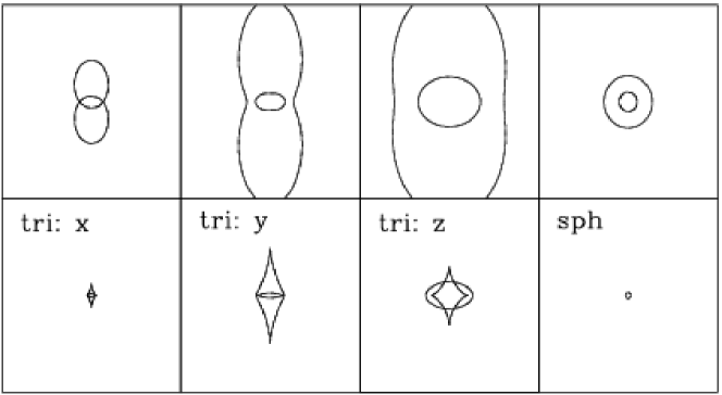
Figure 9: Critical curves (upper) and caustics (lower) of triaxial dark halos projected along three principal vectors (see Figure 7). We consider a halo with mass $M_{\rm vir}=10^{15}h^{-1}M_{\odot}$ and redshift $z=0.3$, and the source plane is placed at $z=2.0$. The axis ratios are fixed to $a/c=0.5$ and $b/c=0.7$. For the concentration parameters, we use the median value given by equation (21). The size of all boxes is the same. The inner slope is $\alpha=1$. The case for the corresponding spherical dark halo is also shown for reference.

One of the most important consequences of the triaxial lens model is that lensing properties are different for different line-of-sight directions, even if the lensing halo is the same. Since strong gravitational lensing is characterized by critical curves and caustics, first we see how they change as we change the direction of the projection.

Figure 9 shows the results. In this Figure, we consider a halo with mass $M_{\rm vir}=10^{15}h^{-1}M_{\odot}$ and redshift $z=0.3$, and the source plane is placed at $z=2.0$. We also fix the axis ratios to $a/c=0.5$ and $b/c=0.7$, which are typical values for the CDM halos (see §2). For the concentration parameters, we use the median value given by equation (21). We show critical curves and caustics of this identical halo projected along three principal vectors. First of all, both sizes and structures of critical curves and caustics are quite different for different projections. The size is the largest when projected along the major axis ($z$), and the smallest along the minor axis ($x$). This is reasonable because the deflection angle is proportional to the surface mass density, i.e., density integrated along the line-of-sight (see Appendix 11), and thus the mass distributions elongated along line-of-sight are expected to have larger deflection angles. Moreover, the size seems larger compared with that of the corresponding (i.e., with the same mass and redshift, and have the median concentration parameter) spherical dark halo. Thus it is expected that triaxiality enhances the number of lenses significantly.

2 Lensing Cross Sections

Figure 10: Distributions of cross sections for multiple images (defined in the lens plane), both for $\alpha=1$ and $1.5$. We consider a halo with mass $M_{\rm vir}=10^{15}h^{-1}M_{\odot}$ and redshift $z=0.3$, and the source plane is placed at $z=2.0$. We took account of PDFs of $a/c$ (eq. [17]), $a/b$ (eq. [18]), and $c_{e}$ (eq. [20]). We assume that the orientations of dark halos are random. Distributions of cross sections for the corresponding spherical dark halo is also shown for reference.

Next we see cross sections for multiple images. Again, we consider a halo with mass $M_{\rm vir}=10^{15}h^{-1}M_{\odot}$ and redshift $z=0.3$, and the source plane is placed at $z=2.0$. This time, however, we do not fix axis ratios but randomly choose them according to their corresponding PDFs (eqs.[17] and [18]). The concentration parameters are also distributed according to the PDF (eq. [20]). The orientations of dark halos are assumed to be random. We also consider the spherical case for reference; in this case the distribution of cross sections are caused only by the PDF of the concentration parameter.

We compute distributions of cross sections both for $\alpha=1$ and $1.5$, which are shown in Figure 10. Most importantly, the triaxiality systematically shifts the distributions toward larger cross sections. The amount of the enhancement depends on the value of $\alpha$, but it is more than one order of magnitude for $\alpha=1$. Therefore, the triaxiality does increase the number (or probability) of strong gravitational lensing, as expected.

Another effect we can read off from this Figure is the comparable (or even shallower) width of the distribution of cross sections with the triaxial dark halo. At first sight, this seems strange because in the triaxial model we incorporate PDFs of axis ratios and orientations, in addition to that of concentration parameters that are also taken into account in the spherical model. In fact, the width is affected by the correlation between axis ratios and concentration parameters; Figure 5 implies that the decrease of cross sections due to smaller concentration parameters tends to be compensated by smaller axis ratios. Therefore a correlation shown in Figure 5 is quite important and should be taken into account in applying the triaxial model to lens statistics.

Chapter 4 Arc Statistics in Triaxial Dark Halos: Theoretical Predictions and Comparison with Observations

1 Introduction

The discovery of a lensed arc in a rich cluster A370 (Lynds & Petrosian 1986; Soucail et al. 1987) opened a direct window to probe the dark mass distribution in clusters of galaxies. Since gravitational lensing phenomena are solely dictated by intervening mass distributions, they are not biased by the luminous objects unlike other conventional observations. Indeed, previous work (Wu & Hammer 1993; Miralda-Escudé 1993a, 1995, 2002; Bartelmann 1996; Hattori, Watanabe, & Yamashita 1997b; Molikawa et al. 1999; Williams, Navarro, & Bartelmann 1999; Meneghetti et al. 2001; Molikawa & Hattori 2001; Oguri, Taruya, & Suto 2001; Gavazzi et al. 2003; Sand et al. 2004; Wambsganss, Bode, & Ostriker 2004; Dalal, Holder, & Hennawi 2004a; Macciò 2004) showed that the number, shapes, and positions of lensed arcs are sensitive to the mass distribution of clusters. For instance, Oguri et al. (2001) calculated the number of arcs using the generalization of the universal density profile proposed by NFW and pointed out that it is extremely sensitive to the inner slope and the concentration parameter of the density profile; the number of arcs changes by more than an order of magnitude among different models that are of cosmological interest. Therefore lensing arc surveys provide an important probe of density profiles of clusters in a manner complementary to the statistics of large-separation lensed quasars (Chapters 5 and 6).

While most previous studies of lensed arcs have aimed at constraining the cosmological parameters (Wu & Mao 1996; Bartelmann et al. 1998; Cooray 1999; Sereno 2002; Golse, Kneib, & Soucail 2002; Bartelmann et al. 2003), we rather focus on extracting information of the density profiles of dark matter halos. Thus we fix cosmological parameters to those of our fiducial concordance model (see Table 1). In fact, arc statistics depend on the assumed set of cosmological parameters in two ways; directly through the geometry of the universe and somewhat indirectly through properties of density profiles which also depend on the cosmology. For instance, Bartelmann et al. (1998) found that the numbers of arcs significantly change among different cosmological models, and concluded that only open CDM models can reproduce the high frequency of observed arcs. Oguri et al. (2001) showed, however, that the result largely comes from the larger concentration parameter of halo profiles in the open CDM model than in the Lambda-dominated CDM model. Thus this may be more related to the small-scale behavior of the CDM model than the “global” effect of the cosmological constant.

The values of cosmological parameters are determined fairly accurately now, thus our primary interest here is to confront the density profiles of dark matter halos with the arc statistics, and thereby we would like even to test the collisionless CDM paradigm. For this purpose, a non-spherical description for the lensing halos is the most essential since cross sections for arcs are quite sensitive to the non-sphericity of mass distribution (Chapter 3; see also Bartelmann, Steinmetz, & Weiss 1995a; Bartelmann 1995b; Meneghetti et al. 2001; Oguri 2002b). Figure 1 demonstrate how large the effects of non-sphericity on arc statistics are. Indeed, previous analytic models adopting spherical lens models failed to reproduce the observed high frequency of arcs (Hattori et al. 1997b; Molikawa et al. 1999).

Recently, new methods to constrain the mass profile of individual clusters also have been developed (Smith et al. 2001; Sand et al. 2002, 2004; Clowe & Schneider 2001, 2002; Gavazzi et al. 2003). Although such methods can measure mass distributions of individual clusters precisely, it may suffer from the special selection function and the scatter around the mean mass distribution. For instances, analysis of clusters only with giant arcs may result in more elongated clusters than average because Jing & Suto (2002) showed that triaxial axis ratios have fairly broad distributions. Therefore it is of great importance to study statistics of lensed arcs which allow us to obtain information on the mean profile.

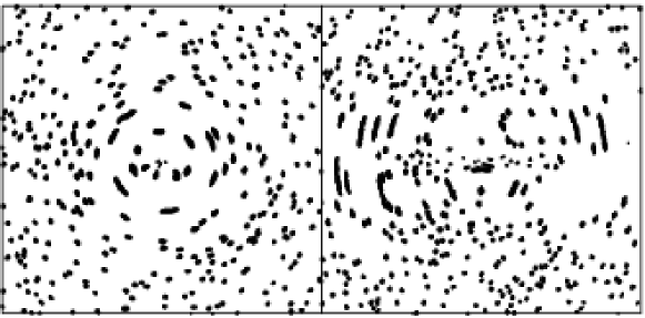
Figure 1: Snapshots of simulated arc images with (right) and without (left) the lens ellipticity, produced from the same spatial distribution of source galaxies. This Figure is taken from Oguri (2002b).

In this chapter, we develop and study in detail, for the first time, such an analytical model of the non-spherical lensing objects for the arc statistics. Specifically we adopt the triaxial description of dark matter halos proposed by Jing & Suto (2002, see Chapter 3). They have presented detailed triaxial modeling of halo density profiles, which enables us to incorporate the asymmetry of dark matter halos statistically and systematically. We first compute the lensing cross sections for arcs on the basis of the Monte Carlo simulations. Then we make systematic predictions of the number of arcs by averaging the cross sections over the probability distribution functions (PDFs) of the axis ratios and the concentration parameters and assuming the random orientation of the dark halos along the line-of-sight of the observer. Those theoretical predictions are compared with the number of observed arcs in a sample of $38$ X-ray selected clusters compiled by Luppino et al. (1999). We pay particular attention to several selection functions of clusters and arcs which may systematically affect our results (e.g., Wambsganss et al. 2004).

2 Modeling the Number of Arcs in Triaxial Dark Halos

1 Cross Sections for Arcs from the Monte Carlo Simulation

First we compute the cross section for arcs without distinguishing tangential and radial arcs mainly because of the computational cost. In fact, the previous analyses indicate that while the number ratio of radial to tangential arcs offers another information on the density profile, the ratio is rather insensitive to the non-sphericity (Molikawa & Hattori 2001; Oguri 2002b).

Since the analytical computation of the cross sections is not practically feasible except for spherical models, we resort to the direct Monte Carlo method (Bartelmann & Weiss 1994; Miralda-Escudé 1993b; Molikawa & Hattori 2001; Oguri 2002b). We showed that the convergence of triaxial dark matter halos is expressed by equation (32). Thus the corresponding lensing deflection angle $\vec{\alpha}$, and therefore the cross section $\tilde{\sigma}$, are fully characterized by the two parameters, $b_{\rm TNFW}$ and $q$, as long as the finite size of source galaxies is safely neglected. Thus we perform the Monte Carlo simulations on the dimensionless $X$-$Y$ plane, where $X$ and $Y$ are $X\equiv x^{\prime}/(R_{0}q_{x})$ and $Y\equiv y^{\prime}/(R_{0}q_{x})$, and tabulate the deflection angle and the dimensionless cross section

$$\vec{\alpha} = \vec{\alpha}(b_{\rm TNFW},q),$$ (1)

$$\tilde{\sigma} = \tilde{\sigma}(b_{\rm TNFW},q),$$ (2)

in $50\times 19$ bins ($\alpha=1$) or $70\times 19$ bins ($\alpha=1.5$) for $b_{\rm TNFW}$ and $q$, respectively. The dimensionless cross section is translated to the dimensional one in the source plane as

$$\sigma=\tilde{\sigma}(b_{\rm TNFW},q)\times\left(R_{0}q_{x}\frac{D_{\rm OS}}{D_{\rm OL}}\right)^{2}.$$ (3)

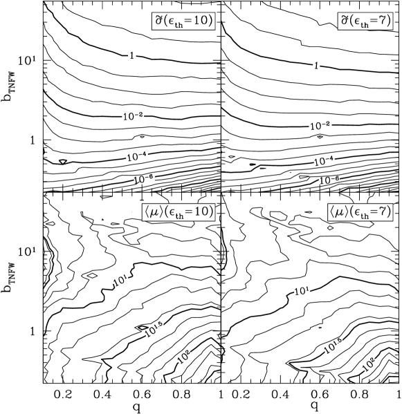
Figure 2: Contours of dimensionless cross sections $\tilde{\sigma}$ and average magnification factors $\langle\mu\rangle$ in the $q$-$b_{\rm TNFW}$ plane for $\alpha=1$. The threshold axis ratios for arcs are set to $\epsilon_{\rm th}=10$ (upper) and $7$ (lower), respectively. Contours are drawn at $10^{0.5n}$ for $\tilde{\sigma}$ and at $10^{0.125n}$ for $\langle\mu\rangle$, where $n$ is integer. When $n$ is in multiples of $4$, contours are drawn by thick lines. These cross sections and magnification factors are derived from Monte Carlo simulations described in §1.

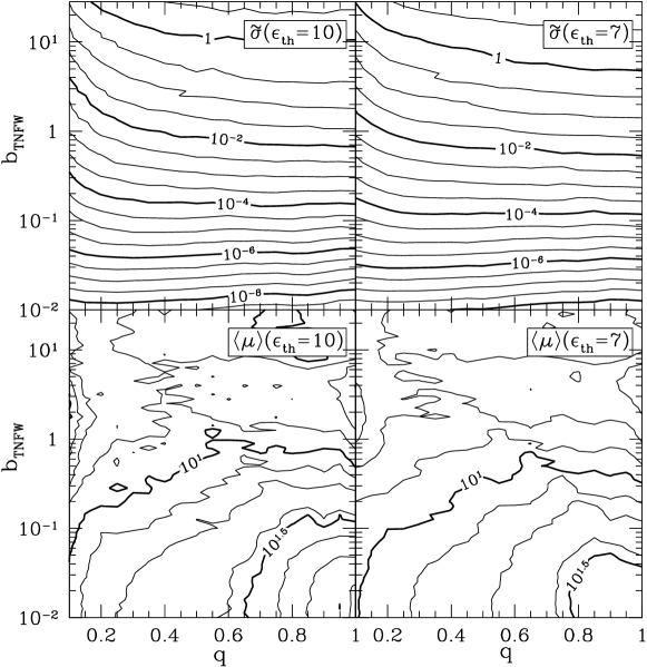
Figure 3: Same as Figure 2, except for $\alpha=1.5$.

We follow the simulation method by Oguri (2002b) which is briefly summarized below. For more details, please see Appendix 12. We use a $2048\times 2048$ regular grid on the $X$-$Y$ plane and calculate the deflection angle at each grid point. The box size is adjusted so as to include all arcs in the box for each $(b_{\rm TNFW},q)$. Therefore, the box size almost scales as the tangential critical line for each $(b_{\rm TNFW},q)$. After those deflection angles are obtained at each grid point, we trace back the corresponding position in the source plane, and see whether or not it constitutes a part of lensed images. In order to take account of the source ellipticity which is also important in arc statistics (Keeton 2001c), we assume that it distributes randomly in the range of [0,0.5], where source ellipticity is defined by $1-b_{\rm s}/a_{\rm s}$ with $a_{\rm s}$ and $b_{\rm s}$ being semi-major and semi-minor axes, respectively. We adopt this distribution of intrinsic ellipticities in order to compare our results with the previous works (e.g., Bartelmann et al. 1998) in which the same distribution was assumed. Moreover, the distribution is roughly consistent with the observed distribution (e.g., Lambas, Maddox, & Loveday 1992). Once we identify a lensed image, we compute its length $l$ and width $w$ as described in Appendix 12. Finally we define a lensed arc if the ratio of $l$ and $w$ exceeds the threshold value $\epsilon_{\rm th}$ that we set:

$$\frac{l}{w}\geq\epsilon_{\rm th}.$$ (4)

In practice, we consider $\epsilon_{\rm th}=7$ and $10$ to check the robustness of the conclusion. We also compute the average magnification of the arcs $\langle\mu\rangle$ for each set of $(b_{\rm TNFW},q)$ which is required in estimating the magnification bias (Turner 1980; Turner, Ostriker, & Gott 1984). The contours of the lensing cross sections and the average magnification are plotted in Figures 2 and 3 for $\alpha=1$ and $\alpha=1.5$, respectively. We confirmed that the cross sections for $q=1$ cases reproduce the analytic result of spherical lens models for point source.

We should note that our current method does not take account of the finite size effect of source galaxies, and thus our results are, strictly speaking, applicable only to a sufficiently small source. Since the number of tangential arcs, which dominates the total number of arcs, is known to be insensitive to the source size (Hattori et al. 1997b; Bartelmann et al. 1998; Molikawa & Hattori 2001; Oguri et al. 2001; Oguri 2002b), this should not change our conclusion.

2 Predicting Numbers of Arcs

The next step is to average the cross section for arcs corresponding to a halo of $M_{\rm vir}$ at $z_{\rm L}$ and a galaxy at $z_{\rm S}$ over the halo properties (its orientations and axis ratios):

$$\overline{\sigma}(M_{\rm vir},z_{\rm L},z_{\rm S})=\int d(a/c)\int dc_{e}\int d(a/b)\int d\theta\int d\phi~{}p(a/c)p(c_{e})p(a/b|a/c)p(\theta)p(\phi)\sigma.$$ (5)

PDFs of axis ratios and concentration parameters are summarized in §2. In what follows, we assume the orientations of triaxial dark matter halos are completely random:

$$p(\theta) = \frac{\sin\theta}{2},$$ (6)

$$p(\phi) = \frac{1}{2\pi}.$$ (7)

The realistic prediction for the number of arcs also requires to properly take account of the magnification bias. Thus we use the average of the cross section times number density of galaxies above the magnitude limit:

$$\overline{\sigma n_{\rm g}}(M_{\rm vir},z_{\rm L},z_{\rm S}) = \int d(a/c)\int dc_{e}\int d(a/b)\int d\theta\int d\phi$$ (9)

$$\times p(a/c)\,p(c_{e})\,p(a/b|a/c)\,p(\theta)\,p(\phi)\,\sigma\int_{L_{\rm min}}^{\infty}dLn_{g}(L,z_{\rm S}),$$

where $n_{g}(L,z)$ is the luminosity function of source galaxies for which we adopt the Schechter form (Schechter 1976):

$$n_{g}(L,z)dL=\phi^{*}\left(\frac{L}{L^{*}}\right)^{\alpha_{\rm s}}\exp\left(-\frac{L}{L^{*}}\right)\frac{dL}{L^{*}}.$$ (10)

Its integral over $L$ simply reduces to

$$\int_{L_{\rm min}}^{\infty}dL\,n_{g}(L,z_{\rm S})=\phi^{*}\Gamma(\alpha_{\rm s}+1,L_{\rm min}/L^{*}),$$ (11)

with $\Gamma(a,x)$ being the incomplete gamma function of the second kind. The lower limit of the integral, $L_{\rm lim}$, may be computed from limiting magnitude of observation, $m^{*}$, and the lensing magnification factor $\langle\mu\rangle$ (see Figures 2 and 3):

$$\frac{L_{\rm min}}{L^{*}} = \frac{10^{-0.4(m_{\rm lim}-m^{*})}}{\langle\mu\rangle},$$ (12)

$$m^{*} = M^{*}+5\log\left[\frac{D_{\rm OS}(1+z_{\rm S})^{2}}{10{\rm pc}}\right]+K(z_{\rm S}).$$ (13)

We adopt the K-correction in B-band for spiral galaxies (King & Ellis 1985):

$$K(z)=-0.05+2.35z+2.55z^{2}-4.89z^{3}+1.85z^{4}.$$ (14)

Finally the number distribution of lensed arcs for a halo of mass $M_{\rm vir}$ at $z_{\rm L}$ is given by

$$\frac{dN_{\rm arc}}{dz_{\rm S}}(z_{\rm S};M_{\rm vir},z_{\rm L})=\overline{\sigma n_{\rm g}}(M_{\rm vir},z_{\rm L},z_{\rm S})\frac{cdt}{dz_{\rm S}}(1+z_{\rm S})^{3},$$ (15)

and the total number of lensed arcs for the halo is

$$N_{\rm arc}(M_{\rm vir},z_{\rm L})=\int_{z_{\rm L}}^{z_{\rm S,max}}dz_{\rm S}\,\frac{dN_{\rm arc}}{dz_{\rm S}}(z_{\rm S};M_{\rm vir},z_{\rm L}).$$ (16)

While the upper limit of redshifts of source galaxies, $z_{\rm S,max}$, is in principle arbitrary, it is practically limited by the validity of the input luminosity function of source galaxies and the applied K-correction at high redshifts. In the present analysis, we conservatively set $z_{\rm S,max}=1.25$ because of the K-correction (eq.[14]) and the luminosity function (§3). Nevertheless we stress here that our methodology can be applied to at higher redshifts if they are replaced by any reliable models valid there.

3 Luminosity Function of Source Galaxies

Name	Model	$z$ Range	$\alpha_{\rm s}$	$M^{*}_{AB}-5\log h{}^{\rm a}$	$\phi^{*}[h^{3}{\rm Mpc^{-3}]}$	Ref.
HDF1	Lambdab	$0.00$ - $0.50{}^{\rm c}$	$-1.19$	$-20.26$	$2.5\times 10^{-2}$	1
		$0.50$ - $0.75$	$-1.19$	$-19.97$	$2.9\times 10^{-2}$
		$0.75$ - $1.25$	$-1.25$	$-20.61$	$1.2\times 10^{-2}$
HDF2	EdSd	$0.00$ - $0.50{}^{\rm c}$	$-1.40$	$-21.20$	$9.0\times 10^{-3}$	2
		$0.50$ - $1.00$	$-1.30$	$-19.90$	$4.2\times 10^{-2}$
		$1.00$ - $1.25$	$-1.60$	$-22.10$	$6.0\times 10^{-3}$
SDF	EdSd	$0.00$ - $1.00{}^{\rm c}$	$-1.07$	$-19.78$	$4.2\times 10^{-2}$	3
		$1.00$ - $1.25$	$-0.92$	$-20.13$	$4.3\times 10^{-2}$
CFRS	EdSd	$0.00$ - $0.50{}^{\rm c}$	$-1.03$	$-19.53$	$2.7\times 10^{-2}$	4
		$0.50$ - $0.75$	$-0.50$	$-19.32$	$6.2\times 10^{-2}$
		$0.75$ - $1.00$	$-1.28$	$-19.73$	$5.4\times 10^{-2}$
		$1.00$ - $1.25{}^{\rm e}$	$-2.50$	$-21.36$	$9.6\times 10^{-4}$

Table 1: B-band luminosity functions of source galaxies used in this paper.
      ^a B-band AB magnitude can be converted to conventional Johnson-Morgan magnitude via $B_{AB}=B-0.14$ (Fukugita, Shimasaku, & Ichikawa 1995).           
      ^b $\Omega_{M}=0.3$, $\Omega_{\Lambda}=0.7$.                                                                           
      ^c Extrapolated to $z=0$.                                                                           
      ^d $\Omega_{M}=1$, $\Omega_{\Lambda}=0$.                                                                           
      ^e The luminosity function for blue galaxies only.                                                                           
      Ref. — (1) Poli et al. 2001; (2) Sawicki et al. 1997; (3) Kashikawa et al. 2003; (4) Lilly et al. 1995

Figure 4: Luminosity functions of source galaxies (eq. [20]) for $z=0.3$, $0.6$, $0.9$, and $1.2$. Parameters of these luminosity functions are summarized in Table 1.

While the predicted number of arcs sensitively depends on the luminosity function of source galaxies (e.g., Hamana & Futamase 1997), $n_{\rm g}(L.z)$ is still fairly uncertain especially at high $z$. Thus we consider the following four luminosity functions measured up to $z=1.25$: HDF1 from the Hubble Deep Field and the New Technology Telescope Deep Field (Poli et al. 2001), HDF2 from the Hubble Deep Field (Sawicki, Lin, & Yee 1997), SDF from the Subaru Deep Field (Kashikawa et al. 2003), and CFRS from the Canada-France Redshift Survey (Lilly et al. 1995). They are summarized in Table 1. Although the Schechter fits to those luminosity functions are valid only at $z>(0.2\sim 0.6)$, we simply extrapolate the values even down to $z=0$ if necessary. This does not affect our result in §3 at all since galaxies at $z\sim 1$ are the main sources of lensed arcs for our sample of clusters at $z>0.2$ (§1).

Except for HDF1, the Schechter parameters were derived assuming the Einstein-de Sitter (EdS) model ($\Omega_{M}=1$, $\Omega_{\Lambda}=0$) in the original references. We convert them into the counterparts in the Lambda-dominated universe ($\Omega_{M}=0.3$, $\Omega_{\Lambda}=0.7$) as follows.

Since the number of galaxies in the redshift interval $[z_{\rm S},z_{\rm S}+dz_{\rm S}]$,

$$dN_{\rm g}(z_{\rm S})\propto D^{2}_{\rm OS}\frac{c\,dt}{dz_{\rm S}}dz_{\rm S}n_{\rm g}(L,z_{\rm S})dL,$$ (17)

is observable, it should be invariant. Thus the luminosity function in the Lambda-dominated universe is related to that in the EdS as:

$$\left[n_{\rm g}(L^{\prime},z_{\rm S})dL^{\prime}\right]_{\rm Lambda}=\frac{\left[D^{2}_{\rm OS}(c\,dt/dz_{\rm S})\right]_{\rm EdS}}{\left[D^{2}_{\rm OS}(c\,dt/dz_{\rm S})\right]_{\rm Lambda}}\left[n_{\rm g}(L,z_{\rm S})dL\right]_{\rm EdS},$$ (18)

where

$$L^{\prime}\equiv\frac{\left[D^{2}_{\rm OS}\right]_{\rm Lambda}}{\left[D^{2}_{\rm OS}\right]_{\rm EdS}}L.$$ (19)

The resulting luminosity functions in terms of the absolute magnitude $M$:

$$\phi_{M}(M,z)dM=0.921\phi^{*}10^{-0.4(\alpha_{\rm s}+1)(M-M^{*})}\exp\left(-10^{-0.4(M-M^{*})}\right)dM,$$ (20)

at $z=0.3$, $0.6$, $0.9$, and $1.2$ are plotted in Figure 4. Clearly the uncertainty increases at fainter luminosities at $z>1$, which may significantly change the predicted number of arcs. Therefore, while we adopt HDF1 as our fiducial model, we also attempt to evaluate the uncertainty due to the different choice of luminosity functions using the other three.

4 Predicted Cross Sections and Numbers of Arcs

Figure 5: Average cross sections (eq. [5]) for triaxial and spherical dark matter halo models as a function of source redshift $z_{\rm S}$ for both $\alpha=1$ (left) and $1.5$ (right), where $\alpha$ is the inner slope of dark matter halo density profile. The lens cluster has a mass $M_{\rm vir}=10^{15}h^{-1}M_{\odot}$ and is placed at $z_{\rm L}=0.3$. For the threshold axis ratio of arcs, we adopt both $\epsilon_{\rm th}=10$ (solid) and $7$ (dashed).

Figure 6: Number distributions of arcs (eq. [15]) for triaxial and spherical dark matter halo models. The B-band magnitude limit for arcs is set to $m_{\rm lim}=24$. The distributions are discontinuous at $z_{\rm S}=0.75$ because we adopt binned luminosity function (see Table 1).

Figure 7: Predicted numbers of arcs (eq. [16]) as a function of halo mass $M_{\rm vir}$. The redshift of the dark halo is still fixed to $z_{\rm L}=0.3$. The B-band magnitude limit for arcs is set to $m_{\rm lim}=24$.

Figure 5 shows the average cross sections (eq. [5]) of a dark matter halo of $M_{\rm vir}=10^{15}h^{-1}M_{\odot}$ at $z_{\rm L}=0.3$. The cross section for the triaxial model is larger by a factor of 10 ($\alpha=1$) and of 4 ($\alpha=1.5$) than that for the spherical counterpart. Since the magnification factor is always larger for smaller cross sections (see Figures 2 and 3), the magnification bias further reduces the difference between $\alpha=1$ and 1.5 for the triaxial model. This explains the behavior of Figure 6 where the source redshift distribution of arcs (eq. [15]) is plotted. Actually the figure indicates that the non-spherical effect even exceeds that of the difference due to the inner slope.

Figures 7, 8 and 9 show how the predicted number of arcs depends on the mass of a lensing halo, the limiting magnitude of the survey, and the adopted luminosity function of source galaxies. Figure 7 shows that the number of arcs is sensitive to the mass of halo, implying the estimate of the mass of the target cluster is essential in interpreting the data. In addition, the difference between $\alpha=1$ and 1.5 becomes smaller for the triaxial model of $M_{\rm vir}>10^{15}M_{\odot}$. Thus in order to distinguish the inner slope clearly as well, one needs a sample of less massive clusters that have lensed arcs.

Figure 8: Predicted numbers of arcs as a function of B-band magnitude limit $m_{\rm lim}$. The mass of lens cluster is $M_{\rm vir}=10^{15}h^{-1}M_{\odot}$.

Figure 9: Predicted numbers of arcs for different luminosity functions of source galaxies as a function of B-band magnitude limit $m_{\rm lim}$. Parameters of luminosity functions are given in Table 1. Only triaxial dark matter halo model and threshold axis ratio $\epsilon_{\rm th}=10$ are considered.

Figure 8 indicates that the number of arcs is also sensitive to the magnitude limit, suggesting that the well-controlled selection function for the arc survey is quite important. On the other hand, the uncertainty of the luminosity function of source galaxies seems to be less critical, at least for arcs of galaxies at $z_{\rm s}<1.25$ that we consider in this paper (Figure 9). The difference among the four luminosity functions (see Table 1) is merely up to 50 % for $m_{\rm lim}<24$, and is within a factor of 2 even at $m_{\rm lim}<26$ except CFRS. The predictions based on HDF1 approximately correspond to the median among the four and this is why we choose this as our fiducial model in what follows.

3 Comparison with the Observed Number of Arcs

1 Cluster Data

We use a sample of $38$ X-ray selected clusters compiled by Luppino et al. (1999). The clusters are selected from the Einstein Observatory Extended Medium Sensitivity Survey (EMSS). For all the clusters, deep imaging observations with B-band limiting magnitude $m_{\rm lim}\sim 26.0$ were carried out to search for arcs.

As we remarked in the previous section, the mass estimate of those clusters is important in understanding the implications from the observed arcs statistics. For this purpose, we first construct a gas temperature – X-ray luminosity (in the Einstein band) relation from a subset of the above clusters whose temperature is determined. Then we estimate the temperature of the remaining clusters using the temperature – luminosity relation. Finally we estimate the mass of each cluster employing the virial mass – gas temperature relation of Finoguenov, Reiprich, & Böhringer (2001).

Figure 10: The luminosity – temperature relation for the EMSS cluster sample. Among 38 clusters, we use 21 clusters with measured temperature to derive luminosity – temperature relation. The best-fit luminosity – temperature relation is shown in equation (21).

		$L_{X}$(EdS)a	$L_{X}$(Lambda)b	$T_{X}$	$M_{\rm vir}$
Name	$z_{\rm L}$	[$10^{44}{\rm erg\,s^{-1}}$]	[$10^{44}{\rm erg\,s^{-1}}$]	[${\rm keV}$]	[$10^{14}h^{-1}M_{\odot}$]	Ref.
MS 0011.7$+$0837	$0.163$	$3.77$	$2.24$	$4.79^{+0.48}_{-0.44}{}^{\rm c}$	$3.89^{+0.72}_{-0.66}$	1
MS 0015.9$+$1609	$0.546$	$14.64$	$11.03$	$8.92^{+0.57}_{-0.56}$	$12.30^{+1.46}_{-1.43}$	1, 2
MS 0302.5$+$1717	$0.425$	$2.88$	$2.04$	$4.62^{+0.45}_{-0.41}{}^{\rm c}$	$3.64^{+0.66}_{-0.60}$	1
MS 0302.7$+$1658	$0.426$	$5.04$	$3.57$	$4.35^{+0.80}_{-0.64}$	$3.25^{+1.11}_{-0.89}$	1, 2
MS 0353.6$-$3642	$0.320$	$5.24$	$3.48$	$6.46^{+0.98}_{-0.80}$	$6.77^{+1.90}_{-1.55}$	1, 2
MS 0433.9$+$0957	$0.159$	$4.34$	$2.57$	$5.04^{+0.53}_{-0.48}{}^{\rm c}$	$4.27^{+0.83}_{-0.75}$	1
MS 0440.5$+$0204	$0.190$	$4.01$	$2.43$	$5.30^{+0.60}_{-0.40}$	$4.69^{+0.98}_{-0.66}$	1, 3
MS 0451.5$+$0250	$0.202$	$6.98$	$4.27$	$8.60^{+0.50}_{-0.50}$	$11.50^{+1.24}_{-1.24}$	1, 3
MS 0451.6$-$0305	$0.539$	$19.98$	$15.00$	$10.27^{+0.85}_{-0.80}$	$15.97^{+2.45}_{-2.30}$	1, 2
MS 0735.6$+$7421	$0.216$	$6.12$	$3.79$	$5.85^{+0.68}_{-0.61}{}^{\rm c}$	$5.63^{+1.21}_{-1.09}$	1
MS 0811.6$+$6301	$0.312$	$2.10$	$1.40$	$4.87^{+0.95}_{-0.63}$	$4.01^{+1.45}_{-0.96}$	1, 2
MS 0839.8$+$2938	$0.194$	$5.35$	$3.25$	$4.20^{+0.20}_{-0.20}$	$3.05^{+0.27}_{-0.27}$	1, 3
MS 0906.5$+$1110	$0.180$	$5.77$	$3.47$	$5.65^{+0.64}_{-0.58}{}^{\rm c}$	$5.28^{+1.11}_{-1.00}$	1
MS 1006.0$+$1201	$0.221$	$4.82$	$2.99$	$5.34^{+0.58}_{-0.52}{}^{\rm c}$	$4.76^{+0.96}_{-0.86}$	1
MS 1008.1$-$1224	$0.301$	$4.49$	$2.95$	$8.21^{+1.15}_{-1.05}$	$10.55^{+2.74}_{-2.50}$	1, 2
MS 1054.5$-$0321	$0.823$	$9.28$	$7.79$	$10.4^{+1.00}_{-1.00}$	$16.35^{+2.91}_{-2.91}$	1, 4
MS 1137.5$+$6625	$0.782$	$7.56$	$6.26$	$5.70^{+0.80}_{-0.60}$	$5.37^{+1.40}_{-1.05}$	1, 5
MS 1147.3$+$1103	$0.303$	$2.30$	$1.51$	$5.96^{+0.99}_{-0.69}$	$5.83^{+1.79}_{-1.25}$	1, 2
MS 1201.5$+$2824	$0.167$	$2.03$	$1.21$	$3.78^{+0.34}_{-0.32}{}^{\rm c}$	$2.51^{+0.42}_{-0.39}$	1
MS 1208.7$+$3928	$0.340$	$2.03$	$1.37$	$3.97^{+0.36}_{-0.33}{}^{\rm c}$	$2.75^{+0.46}_{-0.42}$	1
MS 1224.7$+$2007	$0.327$	$4.61$	$3.08$	$4.09^{+0.65}_{-0.52}$	$2.90^{+0.85}_{-0.68}$	1, 2
MS 1231.3$+$1542	$0.238$	$2.88$	$1.81$	$4.41^{+0.42}_{-0.39}{}^{\rm c}$	$3.34^{+0.59}_{-0.55}$	1
MS 1241.5$+$1710	$0.549$	$10.70$	$8.07$	$6.09^{+1.38}_{-1.14}$	$6.07^{+2.55}_{-2.10}$	1, 2
MS 1244.2$+$7114	$0.225$	$3.84$	$2.39$	$4.90^{+0.50}_{-0.46}{}^{\rm c}$	$4.06^{+0.77}_{-0.71}$	1
MS 1253.9$+$0456	$0.230$	$3.14$	$1.96$	$4.55^{+0.44}_{-0.40}{}^{\rm c}$	$3.54^{+0.63}_{-0.58}$	1
MS 1358.4$+$6245	$0.327$	$10.62$	$7.09$	$7.50^{+4.30}_{-0.91}{}^{\rm d}$	$8.93^{+9.48}_{-2.01}$	1, 2, 6
MS 1426.4$+$0158	$0.320$	$3.71$	$2.47$	$6.38^{+0.98}_{-1.20}$	$6.62^{+1.88}_{-2.30}$	1, 2
MS 1455.0$+$2232	$0.259$	$16.03$	$10.23$	$5.60^{+1.88}_{-1.15}{}^{\rm d}$	$5.20^{+3.23}_{-1.98}$	1, 3, 6
MS 1512.4$+$3647	$0.372$	$4.81$	$3.30$	$3.39^{+0.40}_{-0.35}$	$2.05^{+0.45}_{-0.39}$	1, 2
MS 1546.8$+$1132	$0.226$	$2.94$	$1.83$	$4.43^{+0.43}_{-0.39}{}^{\rm c}$	$3.37^{+0.61}_{-0.55}$	1
MS 1618.9$+$2552	$0.161$	$2.24$	$1.33$	$3.92^{+0.36}_{-0.33}{}^{\rm c}$	$2.68^{+0.46}_{-0.42}$	1
MS 1621.5$+$2640	$0.426$	$4.55$	$3.22$	$6.59^{+0.92}_{-0.81}$	$7.02^{+1.82}_{-1.60}$	1, 2
MS 1910.5$+$6736	$0.246$	$4.39$	$2.78$	$5.20^{+0.55}_{-0.50}{}^{\rm c}$	$4.53^{+0.89}_{-0.81}$	1
MS 2053.7$-$0449	$0.583$	$5.78$	$4.43$	$8.14^{+3.68}_{-2.15}$	$10.39^{+8.70}_{-5.08}$	1, 2
MS 2137.3$-$2353	$0.313$	$15.62$	$10.34$	$5.20^{+1.09}_{-0.42}{}^{\rm d}$	$4.53^{+1.76}_{-0.68}$	1, 2, 6
MS 2255.7$+$2039	$0.288$	$2.04$	$1.33$	$3.92^{+0.36}_{-0.33}{}^{\rm c}$	$2.68^{+0.46}_{-0.42}$	1
MS 2301.3$+$1506	$0.247$	$3.29$	$2.08$	$4.65^{+0.46}_{-0.42}{}^{\rm c}$	$3.68^{+0.67}_{-0.62}$	1
MS 2318.7$-$2328	$0.187$	$6.84$	$4.14$	$6.05^{+0.73}_{-0.65}{}^{\rm c}$	$6.00^{+1.34}_{-1.19}$	1

Table 2: Properties of clusters in the $38$ EMSS distant cluster sample. Errors are at $68$% C.L.
      ^a X-ray luminosity in the $0.3-3.5{\rm keV}$ band for $\Omega_{M}=1$, $\Omega_{\Lambda}=0$, and $h=0.5$ universe.           
      ^b X-ray luminosity in the $0.3-3.5{\rm keV}$ band for $\Omega_{M}=0.3$, $\Omega_{\Lambda}=0.7$, and $h=0.7$ universe.                                                                           
      ^c Estimated from $L_{X}-T_{X}$ relation (eq. [21]).                                                                           
      ^d The effects of cooling flows are corrected.                                                                           
      Ref. — (1) Luppino et al. 1999; (2) Novicki, Sornig, & Henry 2002; (3) Mushotzky & Scharf 1997; (4) Jeltema et al. 2001; (5) Borgani et al. 2001; (6) Allen & Fabian 1998

More specifically, our best-fit luminosity – temperature relation from Figure 10 is

$$T_{X}=T_{X,0}\left(\frac{L_{X}(0.3-3.5{\rm keV})}{10^{44}{\rm erg\,s^{-1}}}\right)^{\gamma},$$ (21)

where $\gamma=0.381\pm 0.052$ and $T_{X,0}=3.52^{+0.32}_{-0.29}{\rm keV}$. The derived luminosity – temperature relation is consistent with recent other estimations (e.g., Ikebe et al. 2002). Neglecting the possible redshift evolution for the luminosity – temperature relation (e.g., Mushotzky & Scharf 1997), we estimate the temperature of those clusters without spectroscopic data as shown in Table 2. The mass – temperature relation that we adopt is

$$T_{X}=2.3{\rm keV}\left(\frac{M_{\rm vir}}{10^{14}h^{-1}M_{\odot}}\right)^{0.54}.$$ (22)

This relation is derived by Shimizu et al. (2003) who converted the result of Finoguenov et al. (2001) in terms of $M_{\rm vir}$ assuming the density profile; the difference between $\alpha=1$ and $1.5$ turned out to be negligible.

2 Observed Number of Arcs

Cluster	$z_{\rm L}$	Arc	$z_{\rm S}$	$l/w$	$m_{\rm arc}$	Notes	Ref.
MS 0302.7$+$1658	$0.426$	A1	$\sim 0.8{}^{\rm a}$	$>18$	$B=23.8$	$\cdots$	1, 2
		A1W	$\cdots$	$>12$	$B=24.9$	$\cdots$
MS 0440.5$+$0204	$0.190$	A1	$0.532$	$>10$	$B=22.9$	$\cdots$	1, 3, 4
		A3	$\cdots$	$>20$	$B=24.0$	$\cdots$
MS 0451.6$-$0305	$0.539$	A1	$\cdots$	$10$	$V=24.6$	$\cdots$	1
MS 1006.0$+$1201	$0.221$	A2$+$A3	$\cdots$	$>20$	$V<22.1$	Candidate	1, 5
		A4	$\cdots$	$12.9$	$V=21.4$	Candidate
MS 1008.1$-$1224	$0.301$	A2	$\cdots$	$10.0$	$B=23.4$	Candidate	1
MS 1358.4$+$6245	$0.328$	A1	$4.92$	$>21$	$\cdots$	$\cdots$	1, 6
MS 1621.5$+$2640	$0.426$	A1	$\cdots$	$>18$	$B=23.1$	$\cdots$	1, 7
MS 1910.5$+$6736	$0.246$	A1	$\cdots$	$10.5$	$R=20.6$	Candidate	1, 5
MS 2053.7$-$0449	$0.583$	AB	$\cdots$	$>22$	$V=22.4$	$\cdots$	1, 7
MS 2137.3$-$2353	$0.313$	A1	$1.501$	$18.1$	$B=22.0$	$\cdots$	1, 8, 9, 10

Table 3: Giant arcs ($l/w>10$) in the $38$ EMSS distant cluster sample.
      ^a Estimated from color of the arc.                                                                           
      Ref. — (1) Luppino et al. 1999; (2) Mathez et al. 1992; (3) Luppino et al. 1993; (4) Gioia et al. 1998 (5); Le Févre et al. 1994; (6) Franx et al. 1997; (7) Luppino & Gioia 1992; (8) Fort et al. 1992; (9) Hammer et al. 1997; (10) Sand et al. 2002

The observed giant arcs ($\epsilon_{\rm th}=10$) in the $38$ EMSS cluster sample are listed in Table 3. The number of arcs in this sample is roughly consistent with more recent data from different cluster samples (Zaritsky & Gonzalez 2003; Gladders et al. 2003). In order to be consistent with our adopted luminosity functions and K-correction of source galaxies, we need to select the arcs with $z<1.25$. In reality, this is quite difficult; most of the observed arcs do not have a measured redshift, while uncertainties of source redshifts may systematically change lensing probabilities. For instance, Wambsganss et al. (2004) explicitly showed that it is important to take correctly account of the source redshift which can change cross sections by an order of magnitude. Moreover four in the list labeled “Candidate” in Table 3 are even controversial and may not be real lensed arcs. Thus we consider the two extreme cases; one is to select only the two arcs with measured redshifts less than 1.25, and the other is to assume that all the arcs without measured redshifts in the list (including the candidates) are located at $z<1.25$. Of course the reality should be somewhere in between, and thus we assume that the range between the two cases well represents the current observational error. This means that the observational error can be greatly reduced if redshifts of all arcs are measured in the future observations.

3 Comparison of Theoretical Predictions with Observations

Figure 11: The number of arcs in the 38 EMSS cluster sample (eq. [23]) as a function of B-band limiting magnitude $m_{\rm lim}$. The threshold axis ratio is $\epsilon_{\rm th}=10$. The observed number of arcs taking account of several uncertainties, which is shown by the shaded region, is discussed in §2.

Finally let us compare our theoretical predictions with the data in detail. Our prediction of the number of arcs is the sum of equation (16) over all the 38 EMSS clusters:

$$N_{\rm EMSS}\equiv\sum^{38}_{i=1}N_{\rm arc}(M_{{\rm vir},i},z_{{\rm L},i}).$$ (23)

We also compute the error of the predicted number of arcs by propagating the mass uncertainty for each cluster (Table 2). Figure 11 shows the number of arcs in the 38 EMSS cluster sample as a function of the B-band limiting magnitude $m_{\rm lim}$. When the B-band magnitude of an arc is not available, we convert its corresponding V- or R-band magnitude into the B-band assuming typical colors of spiral galaxies at $z\sim 1$, $B-V=V-R=1$ (Fukugita et al. 1995).

The important conclusion that we draw from Figure 11 is that the triaxial model in the Lambda-dominated CDM universe with the inner slope of $\alpha=1.5$ successfully reproduces the observed number of arcs, and that the spherical model prediction with $\alpha=1$ fails by a wide margin. Both the triaxial model with $\alpha=1$ and the spherical model with $\alpha=1.5$ are marginal in a sense that the presence of substructure in the dark halo which we ignore in the current method should systematically increase our predicted number of arcs. Indeed Meneghetti, Bartelmann, & Moscardini (2003a) reported that the substructure enhances the number of arcs with $\epsilon_{\rm th}=10$ typically by a factor 2 or 3. This is exactly the amount of enhancement that is required to reconcile those two models with the observation.

We note here that the additional contribution due to galaxies inside a cluster is generally small; Flores, Maller, & Primack (2000) and Meneghetti et al. (2000) found that galaxies increase the number of arcs merely by $\sim$10%. Even a central cD galaxy produces the number of arcs by not more than $\sim$50% (Meneghetti, Bartelmann, & Moscardini 2003b).

4 Discussion

1 Comparison with the previous result

Our result that the halos in a Lambda-dominated CDM universe reproduces the observed number of arcs seems inconsistent with the previous result of Bartelmann et al. (1998) who claimed that only open CDM models can reproduce the observation. One possibility to explain the apparent discrepancy is the difference of the inner profile of halos; we showed that the slope of $\alpha=1.5$ is required to reproduce the observation. This implies that N-body simulations may underestimate the real number of arcs unless they have sufficient spatial resolution. On the other hand, cluster-scale halos may indeed have a shallower inner profile (Jing & Suto 2000a). Therefore this is closely related to the well known problem of the inner slope of CDM dark matter halos (Navarro et al. 1996, 1997; Fukushige & Makino 1997, 2001, 2003; Moore et al. 1999b; Ghigna et al. 2000; Jing & Suto 2000a; Klypin et al. 2001; Power et al. 2003; Fukushige et al. 2004; Hayashi et al. 2004; Navarro et al. 2004), and would need further investigation. Moreover, in reality, the mass estimate for each cluster, the limiting magnitude of source galaxies, and the adopted luminosity function would also affect the prediction in a more complicated fashion, and the further quantitative comparison is not easy at this point.

Figure 12: The number of arcs in the 38 EMSS cluster sample as a function of $A_{e}$ for $m_{\rm lim}=24$. Dash-dotted line indicates the fiducial value for $A_{e}$, $A_{e}=1.1$, in a Lambda-dominated CDM model. Dotted lines suggest possible range of $A_{e}$ with taking account of the enhancement of the concentration parameter in an open CDM model (see text for details).

Nevertheless we can point out the general tendency that open CDM models produce more arcs than Lambda-dominated CDM models because of the larger value of the concentration parameter in the former. Thus it is unlikely that difference between open and Lambda-dominated CDM models results from the “global” effect of the cosmological parameters. In order to show this, we compute the number of arcs as a function of $A_{e}$ still assuming the Lambda-dominated CDM model. Figure 12 plots $N_{\rm EMSS}$ for $m_{\rm lim}=24$ as a function of $A_{e}$. While Jing & Suto (2002) found $A_{e}=1.1$ in a Lambda-dominated CDM models, their fitting formula (see also Bartelmann et al. 1998) tend to predict $\sim 30-40\%$ larger concentration parameter in open CDM models. This enhancement of the concentration parameter corresponds to $A_{e}=1.43\sim 1.53$ if we still assume Lambda-dominated CDM models as a background cosmology. Thus the effect of $A_{e}$ alone increases the number of arc by $\sim 50\%-100\%$ even for triaxial cases, which is qualitatively consistent with the result of Bartelmann et al. (1998).

2 Required Non-sphericity of Lensing Halos

Figure 13: The number of arcs in the 38 EMSS cluster sample for fixed axis ratios of dark matter halos. The B-band limiting magnitude is set to $m_{\rm lim}=24$. Left panel plots the oblate case ($a<b=c$) while right panel is the prolate case ($a=b<c$).

Although we showed that the triaxial halos predicted in the Lambda-dominated CDM model reproduce the observed number of arcs, the analysis employed a series of fairly complicated PDFs for the axial ratios, and it is not so clear what degree of non-sphericity for lensing halos is required to account for the observation. Thus we rather simplify the situation and consider that all halos consist of oblate ($a<b=c$) or prolate ($a=b<c$) halos with a fixed axial ratio. This is equivalent to replacing $p(a/c)$ (eq. [17]) or $p(a/b)$ (eq. [18]) by the corresponding $\delta$-functions. Figure 13 plots the result of this exercise.

The predicted number of arcs is indeed sensitive to the axis ratios of dark matter halos, and prolate halos of $a/c\lesssim 0.5$ in the $\alpha=1.5$ case reproduce the observation. This is basically consistent with the finding of Jing & Suto (2002) for halo properties.

The reason why prolate halos tend to produce the larger number of arcs than oblate halos is explained as follows. Notice first that to keep the mass of dark matter halo invariant with the change of the axial ratio, $b_{\rm TNFW}$ should be approximately proportional to $(ab/c^{2})^{-1}$. Suppose that oblate and prolate halos are projected onto their axisymmetric direction ($x$ for oblate and $z$ for prolate). Then their lensing cross sections should scale as

$$\sigma({\rm oblate}) \propto \tilde{\sigma}((a/c)(a/c)^{-1}b_{\rm TNFW},1)$$ (24)

$$= \tilde{\sigma}(b_{\rm TNFW},1),$$

$$\sigma({\rm prolate}) \propto \left(\frac{a}{c}\right)^{2}\tilde{\sigma}((a/c)^{-2}b_{\rm TNFW},1)$$ (25)

$$= \left(\frac{a}{c}\right)^{2-2\delta}\tilde{\sigma}(b_{\rm TNFW},1),$$

where we assume

$$\tilde{\sigma}(b_{\rm TNFW},q)\propto b_{\rm TNFW}^{\delta}.$$ (26)

Since Figures 2 and 3 suggest $\delta\gtrsim 2$, we find that $\sigma({\rm prolate})\gg\sigma({\rm oblate})$ for $a/c<1$. If those halos are projected along the $y$-direction, on the other hand, their cross sections are almost the same:

$$\sigma({\rm oblate})\sim\sigma({\rm prolate})\propto\left(\frac{a}{c}\right)^{-\delta}\tilde{\sigma}(b_{\rm TNFW},a/c).$$ (27)

The above consideration explains the qualitative difference between oblate and prolate halos, and points out that the elongation along the line-of-sight is also important in the arc statistics as well as the asymmetry of the projected mass density.

3 Are Clusters Equilibrium Dark Matter Halos?

So far we have assumed the one-to-one correspondence between dark matter halos and X-ray clusters. This assumption, however, is definitely over-simplified (Suto 2001, 2003). If “dark clusters” which are often reported from recent weak lensing analyses (Hattori et al. 1997a; Wittman et al. 2001; Miyazaki et al. 2002a) are real, the one-to-one correspondence approximation may be unexpectedly inaccurate. As an extreme possibility, let us suppose that observed X-ray clusters preferentially correspond to halos in equilibrium. According to Jing (2000b), such halos have generally larger concentration parameters and their scatter is small. In order to imitate this situation, we repeat the computation using $A_{e}=1.3$ and the scatter of $0.18$ (Jing 2000b; Jing & Suto 2002). We find that this modified model increases the number of arcs merely by 10%$-$20%. Thus our conclusion remains the same.

4 Sample Variance

Figure 14: The effect of the sample variance. The number of arcs in the 38 EMSS cluster sample is calculated, not being averaged over axis ratios, orientation, and concentration parameters, but using fixed values for each clusters. Axis ratios, orientation, and concentration parameters for each cluster are randomly chosen according to their corresponding PDFs (§2). We calculate 10000 realizations and plot the histogram of frequency. Averaged values are shown by arrows.

The predicted number of arcs for the EMSS cluster that we have presented so far is based on the averaged cross section. This is a reasonably good approximation in the situation that the number of sample clusters is large enough, but in the current sample, its validity is not clear. To examine the sample variance, we re-compute the number of arcs in the 38 EMSS cluster sample without using the average statistics. Instead, we first randomly choose values of the axis ratios, the orientation angles, and the concentration parameters for each cluster according to their corresponding PDFs (§2). Then we sum up the number of arcs for the entire cluster sample. We repeat the procedure 10000 times each for $\alpha=1$ and 1.5, and construct a distribution function of $N_{\rm EMSS}$ as plotted in Figure 14. The resulting 1$\sigma$ sample variance is $\sim$30% for $\alpha=1$ and $\sim$15% for $\alpha=1.5$. Therefore we confirm that the effect of the sample variance does not change our overall conclusion.

5 Summary

We have presented a semi-analytic method to predict the number of lensed arcs, for the first time taking proper account of the triaxiality of lensing halos. We found that Lambda-dominated concordance CDM models successfully reproduce the observed number of arcs of X-ray-selected clusters (Luppino et al. 1999) if the inner slope of the density profile is close to $\alpha=1.5$. Since the spherical models significantly underestimate the expected number of arcs, we conclude that the observed number of arcs indeed requires the non-sphericity of the lensing halos. In fact, the number of arcs is sensitive to the axis ratios of those halos, and the non-sphericity that reproduces the observed number corresponds to the minor to major axis ratios of $\sim 0.5$. This value is perfectly consistent with the findings of Jing & Suto (2002) in the Lambda-dominated CDM models. In this sense, we may even argue that the arc statistics lend strong support for the collisionless CDM paradigm at the mass scale of clusters. As discussed in Meneghetti et al. (2001), self-interacting dark matter models (Spergel & Steinhardt 2000) for instance, are inconsistent with the observed number of arcs not only because they erase the central cusp but because they produce much rounder dark matter halos (see Figure 7). Since we have exhibited that even the current arc surveys have a great impact in testing the collisionless CDM paradigm, larger surveys with well-controlled systematics in near future will unveil the nature of dark matter more precisely.

Chapter 5 Theoretical Predictions for Large-Separation Lensed Quasars with Triaxial Dark Halos

1 Introduction

Since the discovery of the first gravitationally lensed quasar Q0957+561 (Walsh et al. 1979), about 80 strong lens systems have been found so far. All of the lensed quasars have image separations smaller than $7^{\prime\prime}$, and they are lensed by massive galaxies (sometimes with small boosts from surrounding groups or clusters of galaxies). The probability that distant quasars are lensed by intervening galaxies was originally estimated by Turner et al. (1984) to be 0.1%–1%, assuming that galaxies can be modeled as singular isothermal spheres (SIS). This prediction has been verified by several optical and radio lens surveys, such as the HST Snapshot Survey (Bahcall et al. 1992), the Jodrell Bank/Very Large Array Astrometric Survey (JVAS; Patnaik et al. 1992), and the Cosmic Lens All Sky Survey (CLASS; Myers et al. 1995). The lensing probability is sensitive to the volume of the universe, so it can be used to place interesting constraints on the cosmological constant $\Omega_{\Lambda}$ (see Chapter 1).

In contrast, lenses with larger image separations should probe a different deflector population: massive dark matter halos that host groups and clusters of galaxies. Such lenses therefore offer valuable and complementary information on structure formation in the universe, including tests of the CDM paradigm (Narayan & White 1988; Cen et al. 1994; Wambsganss et al. 1995; Kochanek 1995b; Flores & Primack 1996; Nakamura & Suto 1997). So far the observed lack of large-separation lensed quasars has been used to infer that, unlike galaxies, cluster-scale halos cannot be modeled as singular isothermal spheres (Keeton 1998a; Porciani & Madau 2000; Kochanek & White 2001; Keeton & Madau 2001a; Sarbu, Rusin, & Ma 2001; Li & Ostriker 2002, 2003; Oguri 2002c; Ma 2003). The difference can probably be ascribed to baryonic processes: baryonic infall and cooling have significantly modified the total mass distribution in galaxies but not in clusters (e.g., Rees & Ostriker 1977; Blumenthal et al. 1986; Kochanek & White 2001). As a result, large-separation lenses may constrain the density profiles of dark matter halos of cluster more directly than small-separation lenses (Maoz et al. 1997; Keeton 2001b; Wyithe, Turner, & Spergel 2001; Takahashi & Chiba 2001; Li & Ostriker 2002; Oguri et al. 2002a; Oguri 2003c; Huterer & Ma 2004a; Kuhlen, Keeton, & Madau 2004). Alternatively, large-separation lensed quasars may be used to place limits on the abundance of massive halos if the density profiles are specified (Narayan & White 1988; Wambsganss et al. 1995; Kochanek 1995b; Nakamura & Suto 1997; Mortlock & Webster 2000; Oguri 2003c; Chen 2003, 2004; Lopes & Miller 2004). Better yet, the full distribution of lens image separations may provide a systematic diagnostic of baryonic effects from small to large scales in the CDM scenario.

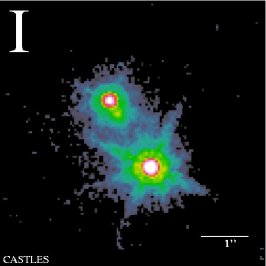
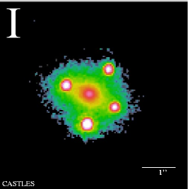
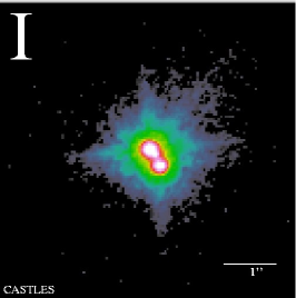
Figure 1: Examples of small-separation lenses with different image multiplicities; double (left), quadruple (center), and naked cusp (right). These Figures are taken from Kochanek et al. (2004b).

In all previous analytic work on the statistics of large-separation lensed quasars, the lens objects were assumed to be spherical. However, in the CDM model dark halos are not spherical at all but triaxial (see Chapter 3). It is already known that triaxiality has a significant effect on the statistics of lensed arcs, from both analytic (see Chapter 4) and numerical (Meneghetti et al. 2003a; Dalal et al. 2004a) points of view. In the statistics of normal lensed quasars, triaxiality (or ellipticity) has been thought to mainly affect the image multiplicities, with only small changes to the total lensing probability (Kochanek 1996; Keeton, Kochanek, & Seljak 1997; Evans & Hunter 2002; Chae 2003; Huterer & Keeton 2004b). However, that conclusion is based on nearly-singular isothermal lens models, and the situation may be quite different for the less concentrated mass distributions of the massive halos that create large-separation lenses. Moreover, only triaxial modeling allows us to study image multiplicities. For the simple mass distribution (i.e., not merging two galaxies, etc.), there are mainly three types of image configurations; double, quadruple, and naked cusp. From the observations of small-separation lensed quasars,it is found that the fraction of double and quadruple lenses is 2:1, and naked cusp lenses are quite rare (see Figure 1). Since image multiplicities depend both on the shape and central concentration of lens objects, and since they are measured easily from observations, they can be a new simple test of the CDM paradigm.

2 Small versus Large Separation Lenses

Before we study large-separation lensed quasars, we review the qualitative differences between small- and large-separation lenses from the theoretical point of view, and see why we concentrate on large-separation lenses.

Figure 2: Comparison of two timescales, $t_{\rm cool}$ (eq. [1]) and $t_{\rm age}$ (eq. [3]), as a function of the virial mass of dark halos $M_{\rm vir}$. Two timescales become equal at $M_{\rm vir}=M_{\rm cool}\sim 10^{13}h^{-1}M_{\odot}$.

First, we see the simple picture of galaxy formation inside dark halos (e.g., Rees & Ostriker 1977; Blumenthal et al. 1986; Kochanek & White 2001). For the gas to collapse and form stars, it must release its internal energy; thus the galaxy formation is governed by the radiative cooling timescale. From the cooling function $\Lambda(T)$ for a plasma (e.g., Sutherland & Dopita 1993), the timescale in the concordance model can be approximated as (Peacock 1999)

$$t_{\rm cool} = \frac{3kT}{2\Lambda(T)n_{b}}$$ (1)

$$\sim 500h^{-2}\left(T_{8}^{-\frac{1}{2}}+0.5T_{8}^{-\frac{3}{2}}\right)^{-1}[{\rm Gyr}],$$

here we assumed the self-similar collapse. The first term ($\Lambda(T)\propto T^{-1/2}$) represents bremsstrahlung, and the second term ($\Lambda(T)\propto T^{-3/2}$) denotes (effectively) atomic line cooling. If we assume that the gas temperature is heated to the virial temperature of dark halos via shocks, $T_{8}\equiv T/(10^{8}K)$ reduces to

$$T_{8}\sim 6\times 10^{-3}\left(\frac{M_{\rm vir}}{10^{12}h^{-1}M_{\odot}}\right)^{2/3}.$$ (2)

Another important timescale is the age of dark halos (i.e., the age of the universe $t_{0}$ minus the formation epoch of dark halos). This can be easily estimated from the formation epoch distribution $dp/dt$ (see, e.g., Lacey & Cole 1993; Kitayama & Suto 1996):

$$t_{\rm age}=t_{0}-\int t\frac{dp}{dt}dt.$$ (3)

Figure 2 shows these timescales, $t_{\rm cool}$ and $t_{\rm age}$, as a function of the virial mass of dark halos $M_{\rm vir}$. It is found that $t_{\rm cool}$ rapidly increases as the virial mass increases. The age $t_{\rm age}$ does not depend on $M_{\rm vir}$ so much, but slightly deceases as the virial mass increases. Thus we can define the characteristic mass $M_{\rm cool}\sim 10^{13}h^{-1}M_{\odot}$, by equating these two time scales, $t_{\rm cool}=t_{\rm age}$: At $M_{\rm vir}<M_{\rm cool}$, baryon cooling takes place efficiently, and galaxies are formed successfully. On the other hand, at $M_{\rm vir}>M_{\rm cool}$ the cooling timescale is so large that baryons are expected to remain mostly in the form of hot gas. This picture naturally explains the qualitative differences between galaxies and clusters. Since the baryon cooling modifies the mass distributions of dark halos significantly and makes them more centrally concentrated (so that it is well approximated by the singular isothermal mass distribution, $\rho(r)\propto r^{-2}$) than original NFW density profile, it does have a great impact also on strong gravitational lensing.

Figure 3: Cumulative distributions of image separation $\theta$, on the basis of the model described by Oguri (2002c). In this model, we adopt the spherical lens objects. For more details of the model, please see the text. All the probabilities are normalized by the CLASS observation at small image separations (Myers et al. 2003; Browne et al. 2003), which is shown by the solid line. The lack of lenses from the explicit search at $6^{\prime\prime}<\theta<15^{\prime\prime}$ in CLASS (Phillips et al. 2001b) is also shown by the horizontal line with an arrow.

Bearing the picture of galaxy formation in mind, one can make a rough prediction for the image separation distributions of strongly lensed quasars (Keeton 1998a; Porciani & Madau 2000; Kochanek & White 2001; Keeton & Madau 2001a; Sarbu, Rusin, & Ma 2001; Li & Ostriker 2002, 2003; Oguri 2002c; Ma 2003). In Figure 3, we plot an example of image separation distributions, calculated from the model described by Oguri (2002c). The model comprises the galaxy formation probability $p_{\rm g}(M)$ (which has a sharp cutoff at $M\sim M_{\rm cool}$) and the ratio of circular velocities of galaxies to virial velocities of dark halos $\gamma\equiv v_{\rm c}/v_{\rm vir}$. In this plot, we choose $\gamma=2$ and adjust $p_{\rm g}(M)$ so as to reproduce the velocity function of galaxies. We simply assume the spherical halos, and adopt the generalized NFW profile with $\alpha=0.5$, $1$, and $1.5$ (see §3). We approximate the mass distribution of galaxies by the singular isothermal sphere:

$$\rho(r)=\frac{\sigma^{2}}{2\pi Gr^{2}},$$ (4)

where one-dimensional velocity dispersion $\sigma$ is related with the circular velocity as $v_{\rm c}=\sqrt{2}\sigma$. All the probabilities are normalized by the CLASS observation at small image separations (Myers et al. 2003; Browne et al. 2003).

It is clear from this Figure that the distributions of image separation $\theta$ have a “break” at around $\theta\sim 7^{\prime\prime}$ which roughly corresponds to $M_{\rm cool}$. The probabilities for large-separation lenses ($\theta\gtrsim 7^{\prime\prime}$) are much smaller than those for small-separation lenses, and depend strongly on the inner slope $\alpha$. Therefore, statistics of large-separation lenses can be a useful tool to probe directly the mass distributions of dark halos, unlike small-separation lenses for which mass distributions of lens objects were significantly modified due to baryon cooling. This argument also justifies lensed arcs in clusters as a direct test of the CDM model.

We note several caveats in calculating image separation distribution from this simple picture of galaxy formation. First of all, the relation between visible galaxies and the hosting dark halos is still uncertain; it has been often assumed that galaxies velocity dispersions are equal to the virial velocities of dark halos (i.e., $\gamma=1$ in the above model), but this is not trivial at all. Actually, some theoretical models, semi-analytic models, and observations do favor $\gamma>1$ (Oguri 2002c, and references therein), and this larger $\gamma$ significantly increases the (relative) probabilities of small-separation lenses. Next, the model of image separation distributions based on dark halos can account for central galaxies (galaxies that lie at the center of dark halos) only; but in reality satellite galaxies (i.e., galaxies in clusters), which are associated with substructures in dark halos, act as lens objects, too. Apparently, these problems come from our poor understanding of galaxy formation, and only affect the relative probabilities of small- and large-separation lenses. Therefore, while full distribution of image separations offer us invaluable information on galaxy formation, theoretical predictions for large separation lenses are robust because abundances and mass distributions of dark halos in the CDM model are accurately known from $N$-body simulations.

3 Modeling Lens Probabilities: Spherical Case

First we briefly review the modeling of lens probabilities with the spherical dark halos which can be done much more easily than the case of the triaxial lens model.

1 Lens Probabilities

Let the physical image position in the lens plane and physical source position in the source plane as $\xi$ and $\eta$, respectively. Consider the probability that a quasar at $z_{\rm S}$ with luminosity $L$ is strongly lensed. The probability of lensing with image separation larger than $\theta$ is given by

$$P(>\!\theta;z_{\rm S},L)=\int_{0}^{z_{\rm S}}dz_{\rm L}\,(1+z_{\rm L})^{3}\,\frac{c\,dt}{dz_{\rm L}}\int_{M(\theta)}^{\infty}dM\,\frac{dn}{dM}\ \sigma_{\rm lens}\ B(z_{\rm S},L)$$ (5)

where

$$\sigma_{\rm lens}=\pi\eta_{\rm r}^{2}\frac{D_{\rm OL}^{2}}{D_{\rm OS}^{2}}$$ (6)

is the cross section for lensing, with $\eta_{\rm r}$ being the physical radius of the radial caustic in the source plane. The lower limit of the mass integral is the mass $M(\theta)$ that corresponds to the image separation $\theta$; this can be computed once the density profile of the lens object is specified. The mass function of dark halos, $dn/dM$, is given in §8.D. The magnification bias $B(z_{\rm S},L)$ is (Turner 1980; Turner et al. 1984)

$$B(z_{\rm S},L)=\frac{2}{\eta_{\rm r}^{2}\,\phi_{L}(z_{\rm S},L)}\int_{0}^{\eta_{\rm r}}d\eta\ \eta\ \phi_{L}(z_{\rm S},L/\mu(\eta))\,\frac{1}{\mu(\eta)},$$ (7)

where $\phi_{L}(z_{\rm S},L)$ is the luminosity function of source quasars. Note that the magnification factor $\mu(\eta)$ may be interpreted as the total magnification or the magnification of the brighter or fainter image, depending on the observational selection criteria (Sasaki & Takahara 1993; Cen et al. 1994). We adopt the magnification of the fainter image, because we concentrate on the large-separation lenses for which the images are completely deblended. Finally, differential distribution can be obtained simply by differentiating equation (5):

$$\frac{dP}{d\theta}(\theta;z_{\rm S},L)=\int_{0}^{z_{\rm S}}dz_{\rm L}\,(1+z_{\rm L})^{3}\,\frac{c\,dt}{dz_{\rm L}}\left[\frac{dM}{d\theta}\frac{dn}{dM}\ \sigma_{\rm lens}\ B(z_{\rm S},L)\right]_{M(\theta)}.$$ (8)

2 Generalized NFW Profile

As discussed, the lensing probability distribution at large-separation reflects the properties of dark halos, rather than galaxies. For the statistics calculation, the debate over the inner slope of the density profile seen in $N$-body simulations leads us to consider the generalized version (Zhao 1996; Jing & Suto 2000a) of the NFW density profile:

$$\rho(r)=\frac{\rho_{\rm crit}(z)\delta_{\rm c}(z)}{\left(r/r_{\rm s}\right)^{\alpha}\left(1+r/r_{\rm s}\right)^{3-\alpha}}.$$ (9)

While the correct value of $\alpha$ is still unclear, the existence of cusps with $1\lesssim\alpha\lesssim 1.5$ has been established in recent $N$-body simulations (Navarro et al. 1996, 1997; Moore et al. 1999b; Ghigna et al. 2000; Jing & Suto 2000a; Klypin et al. 2001; Fukushige & Makino 1997, 2001, 2003; Power et al. 2003; Fukushige et al. 2004; Hayashi et al. 2004). The case $\alpha=1$ corresponds to the original NFW profile, while the case $\alpha=1.5$ resembles the profile proposed by Moore et al. (1999b). The scale radius $r_{\rm s}$ is related to the concentration parameter as

$$c_{\rm vir}=\frac{r_{\rm vir}}{r_{\rm s}}.$$ (10)

Then the characteristic density $\delta_{\rm c}(z)$ is given in terms of the concentration parameter:

$$\delta_{\rm c}(z)=\frac{\Delta_{\rm vir}(z)\Omega(z)}{3}\frac{c_{\rm vir}^{3}}{m(c_{\rm vir})},$$ (11)

where $m(c_{\rm vir})$ is given by equation (12). The mean overdensity $\Delta_{\rm vir}(z)$ can be computed using the nonlinear spherical collapse model (see §8.D).

We define

$$\tilde{\xi} \equiv \xi/r_{\rm s}$$ (12)

$$\tilde{\eta} \equiv \eta D_{\rm OL}/r_{\rm s}D_{\rm OS}.$$ (13)

Then the lensing deflection angle $\alpha(\tilde{\xi})$ is related to the dark halo profile as follows:

$$\alpha(\tilde{\xi})=\frac{b_{\rm NFW}}{\tilde{\xi}}\int_{0}^{\infty}dz\int_{0}^{\tilde{\xi}}dx\frac{x}{\left(\sqrt{x^{2}+z^{2}}\right)^{\alpha}\left(1+\sqrt{x^{2}+z^{2}}\right)^{3-\alpha}}.$$ (14)

The lensing strength parameter $b_{\rm NFW}$ is defined as

$$b_{\rm NFW}\equiv\frac{4\rho_{\rm crit}(z)\delta_{\rm c}(z)r_{\rm s}}{\Sigma_{\rm crit}}.$$ (15)

For sources inside the caustic ($\eta<\eta_{\rm r}$), the lens equation has three solutions $\tilde{\xi}_{1}>\tilde{\xi}_{2}>\tilde{\xi}_{3}$, where image #1 is on the same side of the lens as the source and images #2 and #3 are on the opposite side. The lens image separation is then

$$\theta=\frac{r_{\rm s}(\tilde{\xi}_{1}+\tilde{\xi}_{2})}{D_{\rm OL}}\simeq\frac{2r_{\rm s}\tilde{\xi}_{\rm t}}{D_{\rm OL}},$$ (16)

where $\tilde{\xi}_{\rm t}$ is a radius of the tangential critical curve (Hinshaw & Krauss 1987; Oguri et al. 2002a). The magnification of the fainter image may be approximated by (Oguri et al. 2002a)

$$\mu_{\rm faint}(\eta)\simeq\frac{\tilde{\xi}_{\rm t}}{\tilde{\eta}(1-\alpha^{\prime}(\tilde{\xi}_{\rm t}))}.$$ (17)

These approximations are sufficiently accurate over the range of interest here (see Oguri et al. 2002a). Although it is often adopted in searching for lensed quasars that the flux ratios should be smaller than, e.g., $10:1$, this condition does not affect our theoretical predictions because the flux ratios of strong lensing by NFW halos are typically much smaller than $10:1$ (Oguri et al. 2002a; Rusin 2002).

The concentration parameter $c_{\rm vir}$ depends on a halo’s mass and redshift. Moreover, even halos with the same mass and redshift show significant scatter in the concentration which reflects the difference in formation epoch (Wechsler et al. 2002), and which is well described by a log-normal distribution. For the median of this distribution, we adopt the mass and redshift dependence reported by Bullock et al. (2001) as a canonical model:

$$c_{\rm Bullock}(M,z)=\frac{10}{1+z}\left(\frac{M}{M_{*}(0)}\right)^{-0.13},$$ (18)

where $M_{*}(z)$ is the mass collapsing at redshift $z$ (defined by $\sigma_{M}(z)=\delta_{\rm c}\equiv 1.68$). To study uncertainties related to the concentration distribution we also consider other mass and redshift dependences, e.g.,

$$c_{\rm CHM}(M,z)=10.3(1+z)^{-0.3}\left(\frac{M}{M_{*}(z)}\right)^{-0.24(1+z)^{-0.3}},$$ (19)

from Cooray, Hu, & Miralda-Escudé (2000), and

$$c_{\rm JS}(M,z)=2.44\sqrt{\frac{\Delta_{\rm vir}(z_{c})}{\Delta_{\rm vir}(z)}}\left(\frac{1+z_{c}}{1+z}\right)^{3/2},$$ (20)

from Jing & Suto (2002), with $z_{c}$ being the collapse redshift of the halo of mass $M_{\rm vir}$. Note that these relations were derived under the assumption of $\alpha=1$. We can extend them to $\alpha\neq 1$ by multiplying the concentration by a factor $2-\alpha$ (Keeton & Madau 2001a; Jing & Suto 2002), because it has turned out that dark halos can be fitted reasonably well for $\alpha\neq 1$ only if we apply this translation.

The statistics of large-separation lenses are highly sensitive to the degree of scatter in the concentration (Keeton & Madau 2001a; Wyithe et al. 2001; Kuhlen et al. 2004). Bullock et al. (2001, see also ) found $\sigma_{c}\sim 0.32$ in their simulations. Jing (2000b) found a smaller scatter $\sigma_{c}\sim 0.18$ among well relaxed halos, but Jing & Suto (2002) found $\sigma_{c}\sim 0.3$ if all halos are considered. From these results, it is reasonable to use $\sigma_{c}=0.3$, which is adopted throughout the thesis.

3 Examples

Figure 4: Differential distributions of image separation distributions (eq. [8]). We fix the source at $z=2$ and adopt a power-law luminosity function $\phi_{L}\propto L^{-2.5}$. We use $\alpha=1$ for the fiducial value. Dependences of several parameters are shown; $\Omega_{M}$ (upper left), $\sigma_{8}$ (upper right), and $\alpha$ (lower left). It is also demonstrated how distributions change by adopting different models of concentration parameters (lower right).

Here we show examples of image separation distributions for large-separation lenses, computed from the spherical model described above. In Figure 4, we show image separation distributions and their parameter dependences. We assumed a source at $z=2$ and a power-law luminosity function $\phi_{L}\propto L^{-2.5}$, just for simplicity. As a fiducial model, we consider the spherical halo with $\alpha=1$. Fiducial cosmological parameters are those in Table 1. In each panel, we distribute the parameter we concentrate on, while the other parameters are fixed to fiducial values.

It is found that distributions are sensitive to the inner slope $\alpha$ as well as $\Omega_{M}$ and $\sigma_{8}$. The parameter $\alpha$ determines the cross sections of lensing, while $\Omega_{M}$ and $\sigma_{8}$ changes the abundance of lensing clusters. Probabilities at very large $\theta$ are particularly sensitive to $\sigma_{8}$. We also use three different models of concentration parameters (eqs. [18], [19], and [20]), and show that the uncertainties of concentration parameters result in large differences of lensing probabilities. These are why there have been many attempts to probe the mass distributions and/or abundances of clusters using large-separation lensed quasars.

4 Modeling Lens Probabilities: Triaxial Case

1 Cross sections and image separation distributions

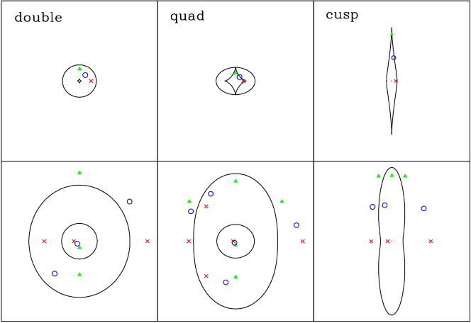
Figure 5: Sample image configurations. The top panels show the source planes, and the bottom panels show the corresponding image planes. The solid lines indicate the caustics and critical curves. We show three sources (denoted by triangles, circles, crosses), and their corresponding images. From left to right, the lenses are doubles, quadruples, and cusps. Specific values of $(b_{\rm TNFW},q)$ for each example are $(2,0.95)$, $(2,0.75)$, and $(0.6,0.25)$ for doubles, quadruples, and cusps, respectively. Doubles and cusps are distinguished by the image parities: doubles have one positive-parity image and one negative-parity image, plus a central double-negative image that is usually too faint to be observed; while cusps have two positive-parity images and one negative parity image, all of comparable brightnesses.

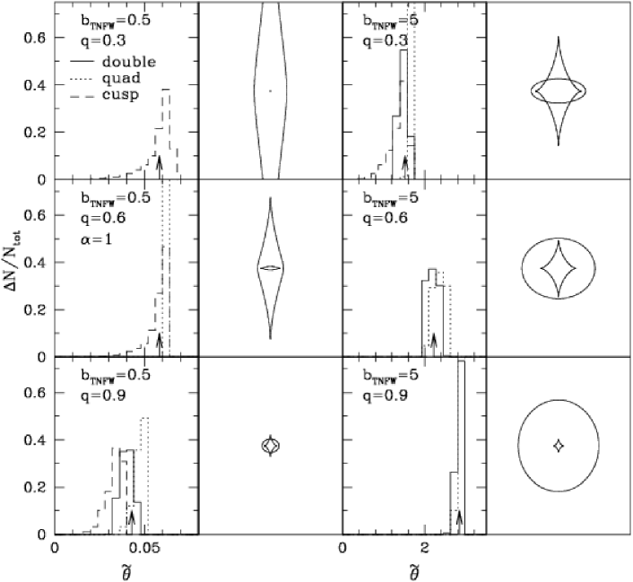
Figure 6: Image separation distributions for sample lenses with $\alpha=1$. Arrows indicate the average separations. The corresponding caustics are shown for reference. For each $b_{\rm TNFW}$, the caustics are all plotted on the same scale.

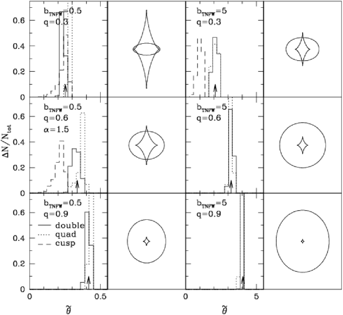
Figure 7: Similar to Figure 6, but for $\alpha=1.5$.

We compute lensing cross sections using Monte Carlo methods. Working in dimensionless coordinates $X\equiv x^{\prime}/L_{0}$ and $Y\equiv y^{\prime}/L_{0}$, we pick random sources and use the gravlens software by Keeton (2001d) to solve the lens equation. Figure 5 shows examples of the three different kinds of image configurations: double, quadruple, and naked cusp lenses. We count the number of sources that produce lenses of different image multiplicities to determine the dimensionless cross sections $\tilde{\sigma}_{2}$, $\tilde{\sigma}_{4}$, and $\tilde{\sigma}_{\rm c}$ for doubles, quadruples, and cusps, respectively. For each set of images, we define the dimensionless image separation $\tilde{\theta}$ to be the maximum separation between any pair of images; this is a convenient definition that depends only on observable quantities and is well defined for all image configurations (no matter how many images there are). We bin the sources by the image separations they produce to derive image separation distributions, as shown in Figures 6 and 7. For a given halo there is a range of separations, but it tends to be fairly narrow ($\lesssim$20%); the main exception is for cusp configurations, which show a tail to small separations that corresponds to sources near the cusp in the caustic. We also plot dimensionless image separations and cross sections in the $b_{\rm TNFW}$-$q$ plane in Figure 8. Hereafter we use the cross sections and image separations tabulated in the range $0.1\leq q\leq 1$ and $10^{-2}\leq b_{\rm TNFW}\leq 10^{2}$.

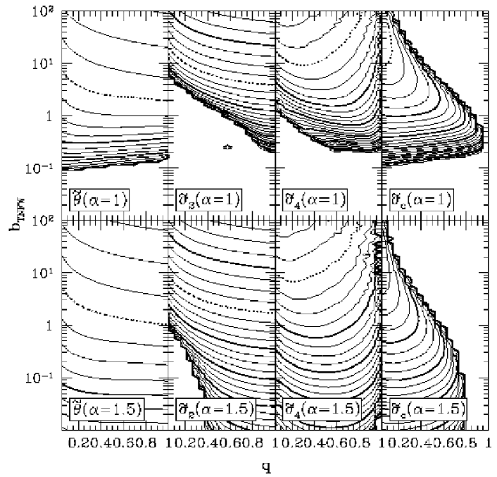
Figure 8: Dimensionless image separations $\tilde{\theta}$ and cross sections $\tilde{\sigma}$ in the $b_{\rm TNFW}$-$q$ plane. The second, third, and fourth panels from left denote cross sections for double lenses, quadruple lenses, and naked cusp lenses, respectively. Dotted lines are contours for $=1$, and thick (thin) solid lines are drawn at $10^{2n}$ ($10^{0.5n}$), where $n$ is integer.

If we not only count the sources but also weight them appropriately, we can compute the magnification bias. Specifically, if the sources have a simple power law luminosity function $\phi_{L}(L)\propto L^{-\beta}$ then the “biased cross section” can be written as

$$B\tilde{\sigma} = \int dXdY\frac{\phi_{L}(L/\mu)/\mu}{\phi_{L}(L)}$$ (21)

$$= \int dXdY\mu^{\beta-1},$$

where the integral is over the multiply-imaged region of the source plane. We can compute the biased cross sections for doubles, quadruples, and cusps similarly. Each source is to be weighted by $\mu^{\beta-1}$, where we take $\mu$ to be the magnification of the second brightest image to reflect the popular method of searching for large-separation lenses in observational data such as the SDSS (see Chapter 6).

An important qualitative result is already apparent from Figure 5. CDM-type dark matter halos are very sensitive to departures from spherical symmetry, in the sense that even small projected ellipticities lead to large tangential caustics and hence large quadruple cross sections. When the ellipticity is large, the tangential caustic is much larger than the radial caustic and nearly all the images correspond to cusp configurations. This situation is notably different from what happens in lensing by galaxies that have concentrated, roughly isothermal mass distributions. In that case, the ellipticity must approach unity before cusp configurations become common (see Keeton et al. 1997; Rusin & Tegmark 2001b). Such large ellipticities are uncommon, and cusp configurations are correspondingly rare among observed galaxy-scale lenses: among $\sim$80 known lenses there is only one candidate (APM 08279+5255; Lewis et al. 2002). The incidence of cusp configurations therefore appears to be a significant distinction between normal and large-separation lenses.

2 Lensing probabilities

The probability that a source at redshift $z_{\rm S}$ is lensed into a system with image separation $\theta$ is computed by summing the biased cross section over an appropriate population of lens halos:

$$\frac{dP}{d\theta}(\theta,z_{\rm S}) = \int dz_{\rm L}\frac{c\,dt}{dz_{\rm L}}(1+z_{\rm L})^{3}\int d(a/c)\int dc_{e}\int d(a/b)\int d\theta\int d\phi$$ (22)

$$\times\left[p(a/c)\,p(c_{e})\,p(a/b|a/c)\,p(\theta)\,p(\phi)\,B\sigma\,\frac{dn}{dM}\right]_{M(\theta)}.$$

The first integral is over the volume between the observer and the source. The next three integrals are over the structural parameters of the lens halos, while the last two integrals cover the different orientations. The mass function of dark halos is represented by $dn/dM$. Finally, $M(\theta)$ is the mass of a halo that produces image separation $\theta$ (for given redshift and other parameters), which is given by the solution of

$$\theta=R_{0}\,q_{x}\,\tilde{\theta}(b_{\rm TNFW},q).$$ (23)

The square brackets in equation (22) indicate that the integrand is to be evaluated only for parameter sets that produce the desired image separation. Equation (22) gives the total lensing probability, but we can simply replace the total biased cross section $B\sigma$ with $B_{2}\sigma_{2}$, $B_{4}\sigma_{4}$, or $B_{c}\sigma_{c}$ to compute the probability for doubles, quadruples, or cusps.

5 Lensing Probabilities and Image Multiplicities in the Triaxial Halo Model

1 Dependence of the triaxiality

Figure 9: Lensing probabilities and image multiplicities as a function of $a/c$. The left panels are for inner slope $\alpha=1$, and the right panels for $\alpha=1.5$. We adopt $\theta=15^{\prime\prime}$, $\beta=2.5$, and $z_{\rm S}=2.0$. We show the total lensing probability (thick solid line), as well as the probabilities for double (dotted), quadruple (dashed), and cusp (dash-dotted) lenses. For comparison, the lensing probability of spherical halos is shown by the thin solid line.

We begin by examining how the lensing probabilities and image multiplicities vary when we change the degree of triaxiality. We remove the integral over $a/c$ in equation (22) to compute the lensing probabilities at fixed triaxiality (we still integrate over the intermediate axis ratio $a/b$ and over random orientations). We can then plot the probabilities as a function of $a/c$, as shown in Figure 9. In this example, we place the source at redshift $z_{\rm S}=2.0$, and we use a source luminosity function with slope $\beta=2.5$. We compute the probabilities for an image separation of $\theta=15^{\prime\prime}$, for concreteness.

For $a/c\to 1$ we recover the spherical case. As $a/c$ decreases (the triaxiality increases), at first the total lensing probability stays roughly constant but the fraction of quadruples rises; this is similar to the effects of ellipticity on isothermal lenses (see Keeton et al. 1997; Rusin & Tegmark 2001b). Then the probability for naked cusp image configurations begins to rise dramatically, and they come to dominate the total probability. Interestingly, the sum of the probabilities for quadruple and double lenses is roughly equal to the probability for spherical halos for most values of $a/c$, at least for this example with image separation $\theta=15^{\prime\prime}$ (also see Figures 10–12 below). This suggests that the enhancement in the total lensing probability is mainly driven by naked cusp configurations. The $\alpha=1$ and 1.5 cases both have these qualitative features, and they differ only in the quantitative details. Since the typical triaxiality in CDM simulations is $a/c\sim 0.5$ (see Figure 4), it appears that triaxiality can have a significant effect on the statistics of large-separation lenses.

2 Full results

Figure 10: Lensing probabilities and image multiplicities with triaxial dark halos as a function of image separation $\theta$. The source is placed at $z_{\rm S}=2.0$, and slope of the source luminosity function is fixed to $\beta=2.5$.

To compute the full impact of triaxiality on lens statistics, we must integrate over an appropriate triaxiality distribution (as in equation 22). Figure 10 shows the resulting lensing probabilities and image multiplicities as a function of the image separation $\theta$. Again, we place the source quasar at $z_{\rm S}=2.0$, and fix the slope of the source luminosity function to $\beta=2.5$. The first important result is that the triaxial model predicts larger lensing probabilities than the spherical model for all image separations. The enhancement is a factor of $\sim$4 for $\alpha=1$, and a factor of $\sim$2 for $\alpha=1.5$, if the image separation is not so large ($\theta\lesssim 30^{\prime\prime}$). At larger separations it seems that the effect of triaxiality is even more significant, especially for $\alpha=1$; we will discuss this issue in §3.

There are several interesting results in the image multiplicities. The $\alpha=1$ and $1.5$ cases have very different multiplicities: with $\alpha=1$ the lensing probability is dominated by cusp configurations; while with $\alpha=1.5$ quadruple lenses are somewhat more common than cusps. Neither result is very sensitive to the image separation. In both cases double lenses are fairly uncommon, which is very different from the situation with normal arcsecond-scale lenses produced by nearly-isothermal galaxies. This result is consistent with previous theoretical conclusions that image multiplicities depend on the central concentration of the lens mass distribution, such that less concentrated profiles tend to produce more quadruple and cusp lenses (Kassiola & Kovner 1993; Kormann, Schneider, & Bartelmann 1994; Rusin & Tegmark 2001b; Evans & Hunter 2002; Dalal et al. 2004a). The important point for observations is that if dark halos have inner profiles with $\alpha\lesssim 1.5$, then many or even most large-separation lenses should be quadruples or cusps rather than doubles. Another point is that the image multiplicities are sensitive to the inner density profile, so they offer a new method for probing dark matter density profiles that is qualitatively different from methods discussed before.

Figure 11: Lensing probabilities and image multiplicities with triaxial dark halos as a function of the slope of the source luminosity function $\beta$. We consider an image separation of $\theta=15^{\prime\prime}$, and we place the source at $z_{\rm S}=2.0$.

Magnification bias is important in lens statistics, particularly in image multiplicities, because it gives more weight to quadruple and cusp configurations (which tend to have large magnifications) than to doubles. We should therefore understand what happens when we modify the magnification bias by varying the slope $\beta$ of the source luminosity function. The results are shown in Figure 11 (for image separation $\theta=15^{\prime\prime}$ and source redshift $z_{\rm S}=2.0$). The lensing probabilities increase as $\beta$ increases, because as the source luminosity function becomes steeper magnification bias becomes stronger. Interestingly, the increase in the total probability due to triaxiality weakens as $\beta$ increases, although the effect is not strong. As for the image multiplicities, $\alpha=1$ halos are always dominated by cusp lenses, although for sufficiently steep luminosity functions quadruples become fairly common. With $\alpha=1.5$ halos, when magnification bias is weak ($\beta\sim 1$) doubles are the most probable, but as magnification bias strengthens ($\beta$ increases) quadruples receive more weight and become the most likely. In practice, the effective values of $\beta$ are larger than $\sim$1.5 for both optical (e.g., Boyle et al. 2000) and radio surveys (e.g., Rusin & Tegmark 2001b), so we expect cusps to dominate for $\alpha=1$ and quadruples to be the most common for $\alpha=1.5$.

Figure 12: Lensing probabilities and image multiplicities as a function of source redshift $z_{\rm S}$. We fix the image separation to $\theta=15^{\prime\prime}$ and the of the source luminosity function to $\beta=2.5$.

Finally, we consider whether the results depend on the source redshift, as shown in Figure 12. The lensing probabilities rise with $z_{\rm S}$, because there is more volume and hence more deflectors between the observer and the source. In addition, geometric effects mean that a given halo can produce a larger image separation when the source is more distant, so the halo mass required to produce a given image separation goes down and the abundance of relevant deflectors goes up. However, the probability increase affects the different image configurations in basically the same way, so the image multiplicities are quite insensitive to the source redshift. Therefore, we conclude that details of the source redshift distribution are not so important for image multiplicities, at least when the source luminosity function has a power law shape.

3 Statistics at larger image separations

In Figure 10, at very large image separations ($\theta\gtrsim 100^{\prime\prime}$) the lensing probabilities in the triaxial halo model are orders of magnitude larger than those in the spherical halo model. In addition, at these very large separations the $\alpha=1$ case produces higher probabilities than the more concentrated $\alpha=1.5$ case. Both features are puzzling and invite careful consideration.

Figure 13: Dependence of the lensing probability on the cutoff in $a/c$. Both $\theta=15^{\prime\prime}$ and $200^{\prime\prime}$ are shown. Filled squares and open circles denote $\alpha=1$ and $1.5$, respectively. The slope of the luminosity function is fixed to $\beta=2.5$.

Figure 13 shows the dependence of total lensing probability on the lower limit of the integral over $a/c$. In the previous calculations, we assumed $(a/c)_{\rm min}=0.1$. This figure shows that for $\theta=15^{\prime\prime}$ the results are quite insensitive to $(a/c)_{\rm min}$, suggesting that the contribution from extremely triaxial halos is negligible. For $\theta=200^{\prime\prime}$, however, the lensing probability rapidly decreases as $(a/c)_{\rm min}$ increases. In other words, the lensing probability at very large image separations seems to be dominated by very small $a/c$, or very large triaxialities.

Results that are dominated by such extreme halos are probably not very reliable. They depend sensitively on both the assumed PDF for the axis ratio $a/c$ (eq. [17]) and the correlation between $a/c$ and the concentration $c_{e}$ (eq. [21]) at very small axis ratios. The fitting forms presented by Jing & Suto (2002) were intended to reproduce the PDF and correlation at $a/c\gtrsim 0.3$ (see Figures 4 and 5), and it is unclear whether they are still accurate at $a/c\sim 0.1$. In addition, even if we know accurate fitting forms, such a situation implies that sample variance (i.e., the effect of the finite number of lensing clusters) may be quite large.

Another ambiguity is the projection effect. Here, we assumed that the density profile (eq. [7]) extends beyond the virial radius, and in projecting along the line of sight we integrated the profile to infinity. Although it is not clear whether we should cut off the profile at the virial radius or not (e.g., Takada & Jain 2003), the effect of the extended profile on the gravitational lensing is not so large for normal dark halos. However, when $a/c$ is small enough, equation (21) indicates that the concentration parameter $c_{e}$ becomes smaller than unity, so the effect of the extended profile outside the virial radius is quite significant. The puzzling feature that the $\alpha=1$ case produces higher probabilities than the $\alpha=1.5$ case at very large separations can be ascribed to the projection effect, because the effect is more significant for shallower density profiles.

Thus, lenses with extremely large image separations are associated with the most extreme dark matter halos, and it may be difficult to make reliable predictions about them. We emphasize, though, that these issues do not apply to lenses with separations $\theta\lesssim 30^{\prime\prime}$, and on these scales we believe our results to be robust.

6 Summary

The dark matter halos predicted by the CDM model are triaxial rather than spherical, which has a significant effect on the statistics of large-separation gravitational lenses. Triaxiality systematically enhances the lensing probability by a factor of $\sim$4 if dark halos have an inner density profile with $\alpha=1$, or a factor of $\sim$2 if $\alpha=1.5$. The effects may be even more dramatic at very large image separations ($\theta\gtrsim 100^{\prime\prime}$), although such lenses are very sensitive to the most triaxial halos and so the predictions are not as reliable. Thus, triaxiality must be added to the list of important systematic effects that need to be included in calculations of large-separation lens statistics. (Some of the other effects are the inner density profile and the shape of the distribution of concentration parameters, as found in §3.)

Triaxial modeling allows us to predict the image multiplicities for large-separation lenses. We found that the multiplicities depend strongly on the density profile: for $\alpha=1$, lenses are dominated by naked cusp image configurations; while for $\alpha=1.5$, quadruple configurations are the most probable. Double lenses, which are dominant among normal arcsecond-scale lenses, are subdominant in both cases. Note that cusp lenses can be distinguished from doubles by the presence of a third image comparable in brightness to the other two, and by the configuration of image positions. The differences can be ascribed to the different mass density profiles, and they indicate that the multiplicities of large-separation lenses will provide a qualitatively new probe of the central density profiles of massive dark matter halos (and hence a new test of CDM).

The prediction that triaxial halos produce significant fractions of quadruple and cusp lenses should be kept in mind when considering samples of candidate large-separation lenses. For example, Miller et al. (2004) found six large-separation double lens candidates in the Two-degree Field (2dF) Quasar Redshift Survey, but no quadruple or cusp lens candidates. Even accounting for small number statistics, our results suggest that such a high fraction of doubles would be inconsistent with CDM at more than 3$\sigma$, and that it would be surprising if many of the six candidates are genuine lens systems.

While our theoretical model is much more realistic than the simple spherical model, we have still made several simplifying assumptions. One is that we have neglected substructure in dark halos. The galaxies in massive cluster halos do not have a large effect on the statistics of lensed arcs (Meneghetti et al. 2000), but it is not obvious whether or not they would affect large-separation lenses. Substructure can affect the image multiplicities for isothermal lenses (Cohn & Kochanek 2004), so it should be considered for CDM halos as well. Another effect we have neglected is the presence of a massive central galaxy in a cluster. Meneghetti et al. (2003b) claim that central galaxies do not have a large effect on arc statistics. However, because our results depend on the inner slope of the density profile, and a central galaxy effectively increases the concentration, this effect should be considered. A third phenomenon we have neglected is cluster merger events. Indeed, mergers can change the shapes of critical curves and caustics substantially, and thus have a great impact on lensing cross sections (Torri et al. 2004). To estimate the effect on large-separation lens statistics, we would need a realistic model of the cluster merger event rate and the physical conditions of merger events. Addressing these various issues to improve the accuracy of the theoretical predictions is beyond the scope of this thesis, but is certainly of interest for future work.

Chapter 6 Discovery of the Large-Separation Lensed Quasar SDSS J1004+4112

1 Introduction

The CDM model naturally predicts the existence of strong gravitational lens systems with image separations of $\sim\!10^{\prime\prime}$ or even larger, as shown in Chapter 5. Observations of massive clusters of galaxies have revealed many systems of “giant arcs” representing lensed images of background galaxies (see Chapter 4). However, until recently all lensed quasars and radio sources had image separations $<\!7^{\prime\prime}$ corresponding to lensing by galaxies, despite some explicit searches for lenses with larger separations.

The fact that clusters have less concentrated mass distributions than galaxies implies that large-separation lensed quasars should be less abundant than small-separation lensed quasars by one or two orders of magnitude (see, e.g., Figure 3). This explains why past surveys have failed to unambiguously identify large-separation lensed quasars (Kochanek, Falco, & Schild 1995a; Maoz et al. 1997; Hewett et al. 1998; Phillips, Browne, & Wilkinson 2001a; Zhdanov & Surdej 2001; Ofek et al. 2001, 2002). For instance, CLASS found 22 small-separation lenses but no large-separation lenses among $\sim$11,000 radio sources (Phillips et al. 2001b). Although several large separation lensed quasar candidates have been found (e.g., Mortlock, Webster, & Francis 1999), they are thought to be physical (unlensed) pairs on the basis of individual observations (e.g., Green et al. 2002) or statistical arguments (Kochanek, Falco, & Muñoz 1999; Rusin 2002). Recently Miller et al. (2004) found 6 candidate lens systems with image separations $\theta>30^{\prime\prime}$ among $\sim$22,000 quasars in the Two-degree Field (2dF) quasar sample. Given the lack of high-resolution spectra and deep imaging for the systems, however, it seems premature to conclude that they are true lens systems. We note that both because the expected number of lenses with such large image separations in the 2dF sample is much less than unity (Oguri 2003c) and because all these candidates are doubles unlike the theoretical prediction (see Chapter 5), these systems would present a severe challenge to standard models if confirmed as lenses. In Figure 1, we show image separation distribution of known lensed quasars so far. There is a cutoff at $\theta\sim 3^{\prime\prime}$, and no lens system has image separation larger than $7^{\prime\prime}$. We summarize the previous large-separation lens searches in Table 1.

To find a first unambiguous large-separation lensed quasar, we started a project to search for large-separation lenses in the quasar sample of the Sloan Digital Sky Survey (SDSS; York et al. 2000). This project complements ongoing searches for small-separation lenses in SDSS (Inada et al. 2003a, 2004a; Inada 2004b; Pindor et al. 2003, 2004; Johnston et al. 2003; Morgan, Snyder, & Reens 2003; Oguri et al. 2004b). The SDSS has completed less than half of its planned observations, but already it contains more than 30,000 quasars and is superior to previous large-separation lens surveys in several ways. The full SDSS sample will comprise $\sim$100,000 quasars, so we ultimately expect to find several large-separation lensed quasars (Keeton & Madau 2001a; Takahashi & Chiba 2001; Li & Ostriker 2002; Kuhlen et al. 2004). One of the most important advantages of the SDSS in searching for large-separation lensed quasars is that imaging in five broad optical bands allows us to select lens candidates quite efficiently (see Appendix 13).

Figure 1: Number distribution of strongly lensed quasars known so far. No confirmed lens system has image separation $\theta>7^{\prime\prime}$. The data are taken from Kochanek et al. (2004b).

Name	Wavelength	$\theta$ Range	# of Quasars	Median $z$	# of Lenses	Ref.
HST Snapshot	optical	$7^{\prime\prime}-50^{\prime\prime}$	$\sim 80$	$\sim 2$	$0$	1
LBQS	optical	$3^{\prime\prime}-10^{\prime\prime}$	$\sim 1,000$	$\sim 1.3$	$0$	2, 3
ARCS	radio	$15^{\prime\prime}-60^{\prime\prime}$	$\sim 1,000$	$\sim 1.3$	$0$	4
CLASS	radio	$6^{\prime\prime}-15^{\prime\prime}$	$\sim 11,000$	$\sim 1.3$	$0$	5
FIRST	radio	$5^{\prime\prime}-30^{\prime\prime}$	$\sim 9,000$	$\sim 1.0$	$0$	6
2dF	optical	$30^{\prime\prime}-200^{\prime\prime}$	$\sim 22,000$	$\sim 1.5$	$>6$ ??	7

Table 1: Surveys for large-separation lensed quasars.                                                             
      Ref. — (1) Maoz et al. 1997; (2) Hewett et al. 1998; (3) Mortlock & Webster 2000; (4) Phillips et al. 2001a; (5) Phillips et al. 2001b; (6) Ofek et al. 2001; (7) Miller et al. 2004

We search for large-separation lensed quasars in a sample of $\sim$30,000 spectroscopically-confirmed SDSS quasars at redshifts $z$ of $0.6-2.3$, a sample larger than those used in any previous searches. Even with this large sample, the expected number of large-separation lensed quasars is of the order of unity. Then we report the discovery of the first large-separation lensed quasar SDSS J1004+4112 at $z=1.73$. The quasar itself turned out to be previously identified in the ROSAT All Sky Survey (Cao, Wei, & Hu 1999) and the Two-Micron All-Sky Survey (Barkhouse & Hall 2001), but was not recognized as a lensed system. In this Chapter, we describe lens search in the SDSS data, and also photometric and spectroscopic follow-up observations of SDSS J1004+4112 in detail. We discuss the spectra of lensed quasar components, including puzzling differences between emission lines seen in the different images. We analyze deep multicolor imaging data to show the existence of a lensing cluster robustly. We also discuss the implications of this system for the statistics of large-separation lenses, using both spherical and triaxial lens models. The mass modeling of this system is of great interest, and we describe it in Appendix 14.

2 Candidate Selection from the SDSS Object Catalog

The SDSS is a survey to image a quarter of the Celestial Sphere at high Galactic latitude and to measure spectra of galaxies and quasars found in the imaging data (Blanton et al. 2003). The dedicated 2.5-meter telescope at Apache Point Observatory (APO) is equipped with a multi-CCD camera (Gunn et al. 1998) with five broad bands centered at $3561$, $4676$, $6176$, $7494$, and $8873$ Å (Fukugita et al. 1996). The imaging data are automatically reduced by a photometric pipeline (Lupton et al. 2001). The astrometric positions are accurate to about $0\farcs 1$ for sources brighter than $r=20.5$ (Pier et al. 2003). The photometric errors are typically less than 0.03 magnitude (Hogg et al. 2001; Smith et al. 2002). The SDSS quasar selection algorithm is presented in Richards et al. (2002). The SDSS spectrographs are used to obtain spectra, covering $3800$–$9200$ Å at a resolution of $1800$–$2100$, for the quasar candidates. The public data releases of the SDSS are described in Stoughton et al. (2002) and Abazajian et al. (2003, 2004). Please refer Appendix 13 for more details.

Figure 2: Redshift distribution of quasars identified by the spectroscopic pipeline in the SDSS. Dashed vertical lines show the redshift cut $0.6<z<2.3$ used for the statistical analysis.

Large-separation lens candidates can be identified from the SDSS data as follows. First, we select objects that were initially identified as quasars by the spectroscopic pipeline. Specifically, among SDSS spectroscopic targets we select all objects that have spectral classification of SPEC_QSO or SPEC_HIZ_QSO with confidence z_conf larger than $0.9$ (see Stoughton et al. 2002, for details of the SDSS spectral codes). Next we check the colors of nearby unresolved sources to see if any of those sources could be an additional quasar image, restricting the lens search to separations $\theta<60^{\prime\prime}$. We define a large-separation lens by $\theta>7^{\prime\prime}$ so that it exceeds the largest image separation lenses found so far: Q0957+561 with $\theta=6\farcs 26$ (Walsh et al. 1979) and RX J0921+4529 with $\theta=6\farcs 97$ (Muñoz et al. 2001), both of which are produced by galaxies in small clusters. We regard the stellar object as a candidate companion image if the following color conditions are satisfied:

$$\left|\Delta(j-k)\right|<3\sigma_{\Delta(j-k)}=3\sqrt{\left(\sigma_{j,{\rm err}}^{2}+\sigma_{k,{\rm err}}^{2}\right)_{\rm quasar}+\left(\sigma_{j,{\rm err}}^{2}+\sigma_{k,{\rm err}}^{2}\right)_{\rm stellar}},$$ (1)

$$\left|\Delta(j-k)\right|<0.1,$$ (2)

$$\left|\Delta i^{*}\right|<2.5,$$ (3)

where $\{j,k\}=\{u^{*},g^{*}\}$, $\{g^{*},r^{*}\}$, $\{r^{*},i^{*}\}$, and $\{i^{*},z^{*}\}$, and $\Delta$ denotes the difference between the spectroscopically identified quasar and the nearby stellar object. Note that this selection criterion is tentative; we still do not know much about large-separation lenses, so selection criteria may evolve as we learn more.

Object	$i^{*}$	$u^{*}-g^{*}$	$g^{*}-r^{*}$	$r^{*}-i^{*}$	$i^{*}-z^{*}$	Redshift
A	$18.46\pm 0.02$	$0.15\pm 0.05$	$-0.03\pm 0.04$	$0.24\pm 0.03$	$0.02\pm 0.05$	$1.7339\pm 0.0001$
B	$18.86\pm 0.06$	$0.18\pm 0.08$	$-0.05\pm 0.08$	$0.23\pm 0.08$	$-0.03\pm 0.09$	$1.7335\pm 0.0001$
C	$19.36\pm 0.03$	$0.03\pm 0.05$	$-0.03\pm 0.04$	$0.38\pm 0.04$	$0.05\pm 0.08$	$1.7341\pm 0.0002$
D	$20.05\pm 0.04$	$0.15\pm 0.09$	$0.15\pm 0.05$	$0.46\pm 0.05$	$0.09\pm 0.13$	$1.7334\pm 0.0003$

Table 2: Magnitudes and colors for the four quasar images, taken from the SDSS photometric data. Redshifts are derived from Ly$\alpha$ lines in the Keck LRIS spectra (see Figure 4).

Object	R.A.(J2000)	Dec.(J2000)	$\Delta$R.A.[arcsec]a	$\Delta$Dec.[arcsec]a
A	10 04 34.794	$+$41 12 39.29	$0.000\pm 0.012$	$0.000\pm 0.012$
B	10 04 34.910	$+$41 12 42.79	$1.301\pm 0.011$	$3.500\pm 0.011$
C	10 04 33.823	$+$41 12 34.82	$-10.961\pm 0.012$	$-4.466\pm 0.012$
D	10 04 34.056	$+$41 12 48.95	$-8.329\pm 0.007$	$9.668\pm 0.007$
G1	10 04 34.170	$+$41 12 43.66	$-7.047\pm 0.053$	$4.374\pm 0.053$

Table 3: Astrometry of SDSS J1004+4112 from the deep imaging data taken with Suprime-Cam (see §2). The absolute coordinates are calibrated using the SDSS data.
      ^a Positions relative to component A.

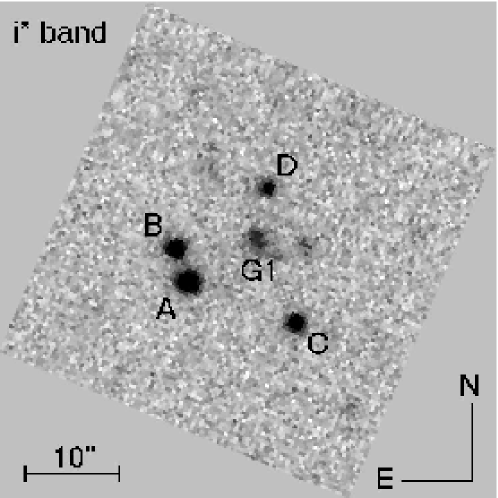
Figure 3: SDSS $i^{*}$-band image of SDSS J1004+4112. Components A, B, C, and D are lensed images while component G1 is the brightest galaxy in the lensing cluster.

Our full sample contains 44,269 quasars with the redshift distribution shown in Figure 2. For the lens search we select the subset of 29,811 quasars with $0.6<z<2.3$, making the redshift cuts for four reasons: (1) at $z<0.6$ quasars are often extended, which can complicated both lens searches and also lens statistics analyses; (2) at $z<0.6$ the sample is contaminated by narrow emission line galaxies; (3) at $z>2.3$ we may miss a number of quasar candidates because of large color errors; and (4) lens statistics calculations for high redshift quasars are not very reliable because of uncertainties in the quasar luminosity function (Wyithe & Loeb 2002a, b). Lens surveys of high-redshift quasars are of course very interesting for insights into the abundance and formation of distant quasars; a search for lenses among high-redshift SDSS quasars is the subject of a separate analysis by Richards et al. (2004a).

SDSS J1004+4112 was first selected as a lens candidate based on a pair of components, A and B (see Figure 3), where B is the SDSS spectroscopic target. Components C and D were identified by visual inspection and found to have colors similar to those of A and B (even though they do not match the above color criteria). Table 2 summarizes the photometry for the four components, and Table 3 gives the astrometry for the four components as well as the galaxy G1 seen in Figure 3. The reason that components C and D have somewhat different colors from B is still unclear, but it must be understood in order to discuss the completeness of the lens survey. The difference might be ascribed to differential absorption or extinction by intervening material (Falco et al. 1999), or to variability in the source on time scales smaller than the time delays between the images (e.g., de Vries, Becker, & White 2003), both of which are effects that become more important as the image separation grows.

3 Data Analysis

1 Spectroscopic Follow-up Observations

Quasar Images

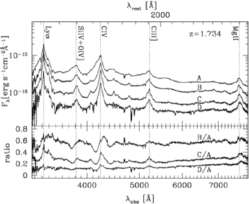
Figure 4: Spectra (top) and flux ratios (bottom) of SDSS J1004+4112 components A, B, C, and D taken with LRIS on Keck I. In the upper panel, we can confirm that all components have Ly$\alpha$, Si 4, C 4, C 3], and Mg 2 emission lines at $z=1.734$. The flux ratios shown in the lower panel are almost constant for a wide range of wavelength. Several absorption lines are also seen in the spectra (see text for details).

Figure 5: Left: The Mg 2 doublet absorption lines (rest frame wavelengths of $2795.5$ Å and $2802.7$ Å, rest frame equivalent width $W_{\rm r}\gtrsim 0.5$ Å) of SDSS J1004+4112 components A, B, C, and D at various wavelengths. The absorption lines are indicated by vertical lines. Right: The C 4 lines of SDSS J1004+4112 components A, B, C, and D taken with LRIS. The associated C 4 doublet absorption lines (rest frame wavelengths $1548.2$ Å and $1550.8$ Å, denoted by dotted lines) are seen in all four components.

Since only component B has a spectrum from SDSS, we obtained spectra of the other components to investigate the lensing hypothesis. The first spectroscopic follow-up observations were done on 2003 May 2 and 5 with the Double Imaging Spectrograph of the Astrophysical Research Consortium (ARC) 3.5-m telescope at APO. All four components have a prominent C 4 emission line ($1549.06$ Å) at $\lambda_{\rm obs}\sim 4230$ Å, indicating that they are quasars with very similar redshifts. Spectra with higher resolution and longer wavelength range were taken on 2003 May 30 with the Low-Resolution Imaging Spectrometer (LRIS; Oke et al. 1995) of the Keck I telescope at the W. M. Keck Observatory on Mauna Kea, Hawaii, USA. The blue grism is 400 line mm^-1, blazed at $3400$ Å, $1.09$ Å pixel^-1, covering $3000$ Å to $5000$ Å. The red grating is 300 line mm^-1, blazed at $5000$ Å, $1.09$ Å pixel^-1, covering $5000$ Å to the red limit of the detector. The spectra were obtained with 900 sec exposures and a $1^{\prime\prime}$ slit in $0\farcs 9$ seeing. The data were reduced in a standard way using IRAF. The Keck/LRIS spectra are shown in Figure 4. All four components show emission lines of Ly$\alpha$, Si 4, C 4, C 3], and Mg 2. They have nearly identical redshifts of $z=1.734$, with velocity differences less than $50\,{\rm km\,s^{-1}}$ (see Table 2). The flux ratios between the images (see Figure 4) are almost constant over the wavelength range 3000–8000 Å, indicating that these are actual lensed images. From the spectra, we conclude that the color differences found in the SDSS images are mainly caused by differences in the emission lines (discussed below) and by slightly different continuum slopes.

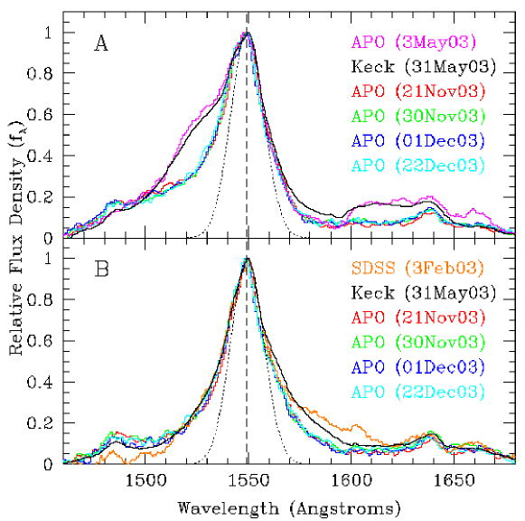
Figure 6: Seven epoch data of C 4 emission lines of components A and B. A power-law continuum is subtracted from each spectrum. The spectra are normalized to the peak of C 4 emission lines. See Richards et al. (2004b) for more details.

Several absorption line systems are seen in the spectra. Components A and D have intervening Mg 2/Fe 2 absorption systems at $z=0.676$; this redshift is similar to that of the foreground galaxies (§1), suggesting that this absorption system is associated with the lensing galaxies. Component D has additional Mg 2 absorption systems at $z=0.726$, $0.749$, $1.083$, $1.226$, and $1.258$. Figure 5 left identifies the various Mg 2 absorbers. We also note that all four components have C 4 absorption lines just blueward of C 4 emission lines (see Figure 5 right). The velocity difference between the emission and absorption lines is $\sim\!500\,{\rm km\,s^{-1}}$, so the absorption system is likely to be associated with the quasar. The fact that all four components have C 4 absorption lines offers further evidence that SDSS J1004+4112 is indeed a gravitational lens.

Figure 5 right shows notable differences in the C 4 emission line profiles in the different components. One possible explanation is the time delay between the lensed images; at any given observed epoch, the images represent different epochs in the source frame. However, the fact that the C 4 emission lines in components A and B differ seems to rule out the time delay explanation: the expected delay is shorter than the month or year time scale on which C 4 emission lines typically vary (e.g., Vanden Berk et al. 2004). Other possible explanations include differences between the viewing angles probed by the images, microlensing amplification of part of the quasar emission region, significant errors in the predicted time delay between A and B, or just that the quasar is extremely unusual.

To resolve this puzzling differences, we obtained additional spectra at different epochs. Figure 6 shows how the strong enhancement in the blue wings of the C 4 emission line was faded. The enhancement lasted at least 28 days, and the predicted time delay between A and B is $\lesssim 30$ days, thus the event is unlikely to be intrinsic to the quasar. The enhancement is seen also in other emission lines, and the amount of the enhancement depends on ionization states so that higher ionization lines tend to be enhanced more. Since the broad emission line region is stratified by ionization and higher ionization lines are found closer to the center (Peterson & Wandel 1999), it is consistent with the interpretation that the enhancement was caused by microlening of part of broad emission line region of the quasar (see Richards et al. 2004b, for more details).

Galaxies

Figure 7: Spectrum of the galaxy G1 taken with LRIS on Keck I. The break, Ca 2 H&K absorption lines, and Mg absorption line are consistent with redshift $z=0.680$ ($z=0.6799\pm 0.0001$ from the Ca 2 H line). The G-band also appears in the spectrum.

Figure 8: Spectra of galaxies G2 and G3 taken with FOCAS on the Subaru 8.2-m telescope. From the absorption lines Ca 2 H&K, H$\delta$, and G-band, we find that the redshifts of both galaxies are $z=0.675$ ($z=0.6751\pm 0.0001$ from the H$\delta$ lines).

The spectrum of the galaxy G1, the brightest object near the center of the quasar configuration (see Figure 3), was acquired on 2003 May 30 with LRIS. The spectrum measured from a 900 sec exposure is shown in Figure 7. We confirm the break and Ca 2 H&K lines at $\lambda_{\rm obs}\sim 6700$ Å. The G-band also appears in the spectrum. From the Ca 2 H&K and Mg lines we derive the redshift of G1 as $z=0.680$.

The spectra of two additional galaxies near G1 (see §2) were taken on 2003 June 20 with the Faint Object Camera and Spectrograph (FOCAS; Kashikawa et al. 2002) on the Subaru 8.2-m telescope of the National Astronomical Observatory of Japan on Mauna Kea, Hawaii, USA. We used the 300B grism together with the SY47 filter, and took optical spectra covering $4100$ Å to $10000$ Å with resolution $2.84$ Å pixel^-1. The seeing was $0\farcs 7$, and the exposure time was 1740 sec for both galaxies. The data were reduced in a standard way using IRAF. The spectra are shown in Figure 8. Both galaxies, denoted as G2 and G3, have $z=0.675$, only $\sim\!700\,{\rm km\,s^{-1}}$ from the redshift of G1.

2 Imaging Follow-up Observations

Observations

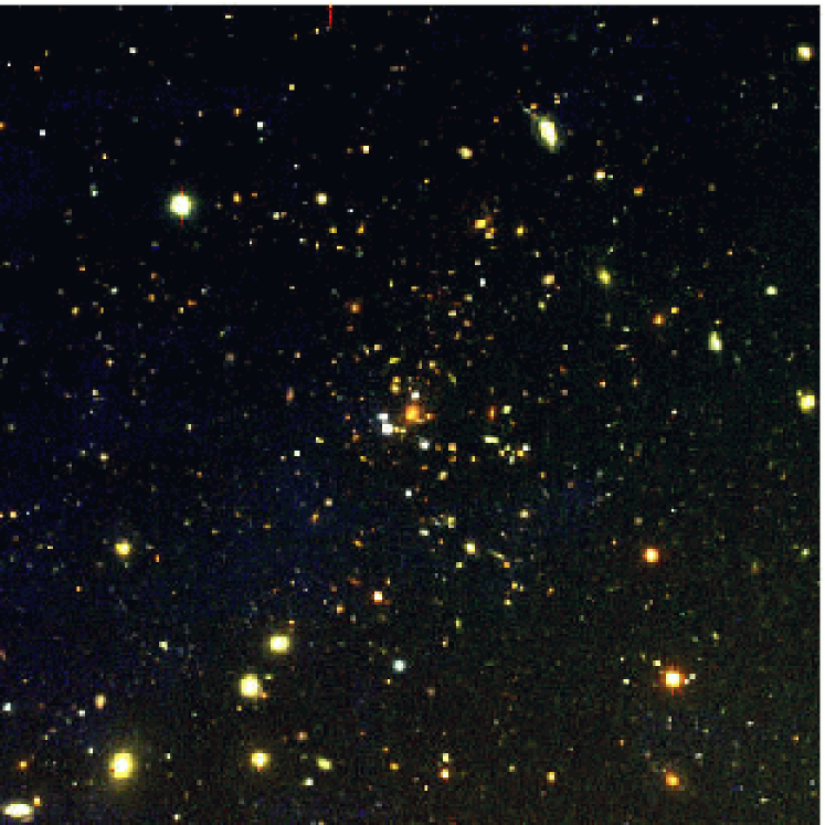
Figure 9: The $gri$ composite Subaru image of the field around SDSS J1004+4112. Many faint galaxies can be seen — their positions and colors are consistent with being members of a cluster ($z=0.68$) centered on component G1.

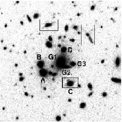
Figure 10: The central region of the Suprime-Cam $i$-band image. The galaxies with measured redshifts (G1 from LRIS and G2 and G3 from FOCAS) as well as the four lensed images are labeled. The possible lensed arclets are marked with rectangles.

Band	Exptime	$m_{\rm lim}$ a
$g$	810	27.0
$r$	1210	26.9
$i$	1340	26.2
$z$	180	24.0

Table 4: Total exposure time in seconds (exptime) and limiting magnitude ($m_{\rm lim}$) for the Subaru deep imaging observations.
      ^a Defined by $S/N>5$ for point sources.                                                                            

A deep $r$-band image of SDSS J1004+4112 was taken on 2003 May 5 with the Seaver Prototype Imaging camera of the ARC 3.5-m telescope at APO. The image shows rich structure, with many galaxies between and around the quasar components suggesting a possible galaxy cluster in the field. For a further check, we obtained deeper multi-color ($griz$) images on 2003 May 28 with the Subaru Prime Focus Camera (Suprime-Cam; Miyazaki et al. 2002b) on the Subaru 8.2-m telescope. The exposure times and limiting magnitudes of the Suprime-Cam images are given in Table 4. Suprime-Cam has a pixel scale of $0\farcs 2\,{\rm pixel^{-1}}$, and the seeing was $0\farcs 5$–$0\farcs 6$. The frames were reduced (bias-subtracted and flat-field corrected) in a standard way. The resulting images are shown in Figure 9. It is clear that there are many red galaxies around the four images. Moreover, we find three possible lensed arclets (distorted images of galaxies behind the cluster), which are shown in Figure 10. The fact that the arclets are relatively blue compared with the brighter galaxies in the field (see Figure 9) suggests that the arclets may be images of distant galaxies (e.g., Colley, Tyson, & Turner 1996). Confirming that they are lensed images will require higher resolution images and measurements of the arclets’ redshifts. If the hypothesis is confirmed, the arclets will provide important additional constraints on the lens mass distribution.

Colors of Nearby Galaxies

The colors of galaxies in the vicinity of SDSS J1004+4112 can help us search for the signature of a cluster. The central regions of clusters are dominated by early-type galaxies (e.g., Dressler 1980) that show tight correlations among their photometric properties (Bower, Lucey, & Ellis 1992). These correlations make it possible to search for clusters using color-magnitude and/or color-color diagrams (Dressler & Gunn 1992; Gladders & Yee 2000; Goto et al. 2002).

We measure the colors of galaxies using the deep Suprime-Cam $griz$ images. Object identifications are performed using the Source Extractor algorithm (SExtractor; Bertin & Arnouts 1996); we identify objects with SExtractor parameter CLASS_STAR smaller than 0.6 in the $i$ band image as galaxies. Note that this star/galaxy separation criterion is successful only for objects with $i\lesssim 24$. The magnitudes in the images are calibrated using nearby stars whose magnitudes are taken from the SDSS photometric data.

Figure 11: Color-magnitude diagrams for the SDSS J1004+4112 field taken with Suprime-Cam. We divide the galaxies into three categories according to their positions: filled circles denote galaxies inside a $40^{\prime\prime}\times 40^{\prime\prime}$ box centered on G1, open triangles denote galaxies inside a $100^{\prime\prime}\times 100^{\prime\prime}$ box, and crosses denote galaxies inside a $200^{\prime\prime}\times 200^{\prime\prime}$ box. These box sizes correspond to $0.2h^{-1}\,{\rm Mpc}\times 0.2h^{-1}{\rm Mpc}$, $0.5h^{-1}{\rm Mpc}\times 0.5h^{-1}{\rm Mpc}$, and $1.0h^{-1}{\rm Mpc}\times 1.0h^{-1}{\rm Mpc}$ at $z=0.68$, respectively. Three spectroscopically confirmed member galaxies are marked with open circles. The corresponding $r$-band absolute magnitudes at $z=0.68$ (without K-correction) are given at the top of the frame.

Figure 12: The $g-r-i$ and $r-i-z$ color-color diagrams of galaxies brighter than $i=24$. Symbols are the same as in Figure 11. Dotted lines indicate color cuts to find cluster members.

Since the red galaxies in clusters are dominant in the central regions, and the center of the cluster is thought to be near G1, we divide the galaxies in the field into three categories: galaxies inside a $40^{\prime\prime}\times 40^{\prime\prime}$ (corresponding to $0.2h^{-1}{\rm Mpc}\times 0.2h^{-1}{\rm Mpc}$ at $z=0.68$) box centered on G1; galaxies inside a $100^{\prime\prime}\times 100^{\prime\prime}$ ($0.5h^{-1}{\rm Mpc}\times 0.5h^{-1}{\rm Mpc}$) box (except for those in the first category); and galaxies inside a $200^{\prime\prime}\times 200^{\prime\prime}$ ($1.0h^{-1}{\rm Mpc}\times 1.0h^{-1}{\rm Mpc}$) box (except for those in the first two categories). Figure 11 shows color-magnitude diagrams for the three categories. It is clear that the color-magnitude relations, particularly $r-i$ and $i-z$, show tight correlations for galaxies inside the $40^{\prime\prime}\times 40^{\prime\prime}$ box. Ridge lines at $r-i\sim 1.1$ and $i-z\sim 0.5$ strongly suggest a cluster of galaxies at $z\sim 0.6$ (Goto et al. 2002). The result is consistent with the Keck and Subaru spectroscopic results showing that the redshifts of galaxies G1, G2, and G3 are all $z\sim 0.68$.

Figure 13: Distributions of galaxies brighter than $i=24$ with (right) and without (left) the color cut. The origin $(0,0)$ is set to the position of the central galaxy G1. Filled squares denote the four lensed images.

We identify cluster members by their location in color-color space (Dressler & Gunn 1992; Goto et al. 2002). We show $g-r-i$ and $r-i-z$ color-color diagrams in Figure 12. We restrict the plots to galaxies brighter than $i=24$ because of the limitation of the star/galaxy separation. We make color-color cuts based on the colors expected of elliptical galaxies (Fukugita et al. 1995): $g-r>1.5$, $r-i>0.7$, and $i-z>0.2$ for elliptical galaxies at $z\gtrsim 0.5$. The galaxy distributions with and without the color cuts are shown in Figure 13. The galaxies that survive the color cuts are concentrated around G1, so we conclude that they are candidate members of a cluster of galaxies at $z=0.68$ whose center is near G1. We note that the distribution of candidate cluster members is not spherical and appears to be elongated North–South.

4 Lens Statistics with Spherical Dark Halos

In this section, we calculate the expected rate of large-separation lensing in the SDSS quasar sample. The discovery of SDSS J1004+4112 allows us to move past the upper limits obtained from previous large-separation lens searches, although at present we focus on testing whether the detection of one large-separation lens in the current sample is consistent with standard theoretical models in the CDM scenario. In this section, we perform a traditional analysis with the spherical lens model.

1 Number of Lensed Quasars in the SDSS

Because the lensing probability depends on the source redshift and luminosity, we compute the predicted number of lenses in redshift and luminosity bins and then sum the bins. Specifically, let $N(z_{j},i^{*}_{k})$ by the number of quasars in a redshift range $z_{j}-\Delta z/2<z<z_{j}+\Delta z/2$ that have a magnitude in the range $i^{*}_{k}-\Delta i^{*}/2<i^{*}<i^{*}_{k}+\Delta i^{*}/2$. Then the predicted total number of lensed quasars is

$$N_{\rm lens}(>\!\theta)=\sum_{z_{j}}\sum_{i^{*}_{k}}N(z_{j},i^{*}_{k})\,P(>\!\theta;z_{j},L(i^{*}_{k})).$$ (4)

We adopt bins of width $\Delta z=0.1$ and $\Delta i^{*}=0.2$. The quasar sample we used comprises 29,811 quasars with mean redshift $\langle z\rangle=1.45$ (see Figure 2).

Figure 14: The cross-filter K-correction, computed from the SDSS composite quasar spectrum created by Vanden Berk et al. (2001). Dotted line indicate the approximation (eq. [5]) with $\alpha_{\rm s}=0.5$.

To calculate the $B$-band absolute luminosity $L(i^{*})$ corresponding to observed magnitude $i^{*}$, we must estimate the cross-filter K-correction $K_{Bi}(z)$. The K-correction calculated from the composite quasar spectrum created from the SDSS sample by Vanden Berk et al. (2001) is shown in Figure 14. As a simplification, one might use the following approximation:

$$K_{Bi}(z)=-2.5(1-\alpha_{\rm s})\log(1+z)-2.5\alpha_{\rm s}\log\left(\frac{7500}{4400}\right)-0.12,$$ (5)

where the offset 0.12 mainly arises from the difference between $AB(4400)$ and $B$ magnitudes (calculated assuming $\alpha_{\rm s}=0.5$; Schmidt, Schneider, & Gunn 1995). Here we use the K-correction directly calculated from composite quasar spectrum.

The luminosity function of quasars is needed to compute magnification bias. We adopt the standard double power law $B$-band luminosity function (Boyle, Shanks, & Peterson 1988)

$$\phi_{L}(z_{\rm S},L)dL=\frac{\phi_{*}}{[L/L_{*}(z_{\rm S})]^{\beta_{l}}+[L/L_{*}(z_{\rm S})]^{\beta_{h}}}\frac{dL}{L_{*}(z_{\rm S})}.$$ (6)

As a fiducial model of the evolution of the break luminosity, we assume the form proposed by Madau, Haardt, & Rees (1999),

$$L_{*}(z_{\rm S})=L_{*}(0)(1+z_{\rm S})^{\alpha_{\rm s}-1}\frac{e^{\zeta z_{\rm S}}(1+e^{\xi z_{*}})}{e^{\xi z_{\rm S}}+e^{\xi z_{*}}},$$ (7)

where a power-law spectral distribution for quasar spectrum has been assumed, $f_{\nu}\propto\nu^{-\alpha_{\rm s}}$. Wyithe & Loeb (2002b) determined the parameters so as to reproduce the low-redshift luminosity function as well as the space density of high-redshift quasars for a model with $\beta_{h}=3.43$ below $z_{\rm S}=3$, $\beta_{h}=2.58$ above $z_{\rm S}=3$, and $\beta_{l}=1.64$. The resulting parameters are $\phi_{*}=624\,{\rm Gpc^{-3}}$, $L_{*}(0)=1.50\times 10^{11}~{}L_{\odot}$, $z_{*}=1.60$, $\zeta=2.65$, and $\xi=3.30$. We call this model LF1. To estimate the systematic effect, we also use another quasar luminosity function (LF2) derived by Boyle et al. (2000): $\beta_{h}=3.41$, $\beta_{l}=1.58$ and an evolution of the break luminosity $L_{*}(z_{\rm S})=L_{*}(0)10^{k_{1}z_{\rm S}+k_{2}z_{\rm S}^{2}}$ with $k_{1}=1.36$, $k_{2}=-0.27$, and $M_{*}=-21.15+5\log h$.

2 Results

Figure 15: Conditional probability distributions for the lens redshift and mass in SDSS J1004+4112, given the image separation $\sim 14^{\prime\prime}$, source redshift $z_{\rm S}=1.739$, and apparent magnitude $i^{*}=18.86$. Solid and dashed lines show the probability distributions with $\alpha=1.5$ and $1.0$, respectively. The arrow shows the measured redshift of the lensing cluster.

First we show the conditional probability distributions

$$\frac{dP}{dz_{\rm L}}(z_{\rm L}|\theta,z_{\rm S},L)\equiv\left|\frac{d^{2}P/dz_{\rm L}d\theta}{dP/d\theta}\right|,$$ (8)

$$\frac{dP}{d\ln M}(M|\theta,z_{\rm S},L)\equiv\left|\frac{d^{2}P/d\ln Md\theta}{dP/d\theta}\right|,$$ (9)

in order to identify the statistically reasonable ranges of redshift and mass for the lensing cluster. Figure 15 shows the conditional probability distributions for the lens redshift and lens mass, given that the gravitational lens system SDSS J1004+4112 has image separation $\sim\!14^{\prime\prime}$, source redshift $z_{\rm S}=1.734$, and apparent magnitude $i^{*}=18.86$. We find the most probable lens redshift to be $z_{\rm L}\sim 0.5$, but the distribution is broad and the measured redshift $z_{\rm L}=0.68$ is fully consistent with the distribution. We also find a cluster mass $M\sim 2$–$3\times 10^{14}\,h^{-1}\,M_{\odot}$ to be most probable for this system. Note that we do not include information on the measured redshift $z_{\rm L}=0.68$ in the conditional probability distributions for the lens mass in Figure 15, which might cause a slight underestimate of the lens mass.

Next we consider the statistical implications of SDSS J1004+4112. Although our large-separation lens search is still preliminary, and we have several other candidates from the current SDSS sample that still need follow-up observations, we can say that the current sample contains at least one large-separation lens system. This is enough for useful constraints because of the complementary constraints available from the lack of large-separation lenses in previous lens surveys. Among the previous large-separation lens surveys, we adopt the CLASS $6^{\prime\prime}<\theta<15^{\prime\prime}$ survey comprising a statistically complete sample of 9,284 flat-spectrum radio sources (Phillips et al. 2001b). For the CLASS sample, we use a source redshift $z_{\rm S}=1.3$ (Marlow et al. 2000) and a flux distribution $N(S)dS\propto S^{-2.1}dS$ (Phillips et al. 2001b) to compute the expected number of large-separation lenses.

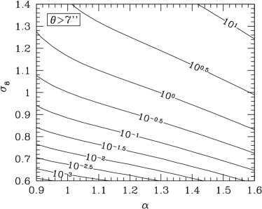
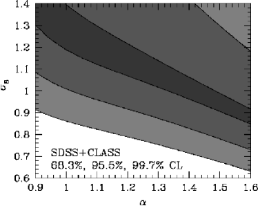
Figure 16: Left: Contours of the predicted number of large-separation ($\theta>7^{\prime\prime}$) lenses in the current SDSS sample in the $(\alpha,\sigma_{8})$ plane. Right: Constraints from both SDSS and CLASS in the $(\alpha,\sigma_{8})$ plane. The discovery of one large-separation ($\theta>7^{\prime\prime}$) lens in SDSS provides lower limits on $\alpha$ and $\sigma_{8}$, while the lack of large-separation lenses ($6^{\prime\prime}<\theta<15^{\prime\prime}$) in CLASS yields the upper limit. The regions in which both SDSS and CLASS limits are satisfied are shown by the shadings. The confidence levels are $68.3\%$, $95.5\%$, and $99.7\%$ in the dark, medium, and light shaded regions, respectively. Both plots are based on the spherical lens model.

Figure 16 shows contours of the predicted number of large-separation lenses with $\theta>7^{\prime\prime}$ in the SDSS quasar sample. Since the number of lenses is very sensitive to both the inner slope of the density profile $\alpha$ and the mass fluctuation normalization $\sigma_{8}$ (e.g., Oguri 2003c), we draw contours in the $(\alpha,\sigma_{8})$ plane. Constraints from the existence of SDSS J1004+4112 together with the lack of large-separation lenses in the CLASS sample are also shown in Figure 16. To explain both observations, we need a relatively large $\alpha$ or $\sigma_{8}$, such as $\sigma_{8}=0.95^{+0.35}_{-0.2}$ (95% confidence) for $\alpha=1.5$. This value is fully consistent with other observations (see Table 6). By contrast, if we adopt $\alpha=1$ then the required value of $\sigma_{8}$ is quite large, $\sigma_{8}\gtrsim 1.2$. Thus, our result might be interpreted as implying that dark matter halos have cusps steeper than $\alpha=1$. Alternatives to collisionless CDM, such as self-interacting dark matter (Spergel & Steinhardt 2000) or warm dark matter (Colín, Avila-Reese, & Valenzuela 2000; Bode, Ostriker, & Turok 2001), tend to produce less concentrated mass distributions which are effectively expressed by low $\alpha$; such models would fail to explain the discovery of SDSS J1004+4112 unless $\sigma_{8}$ is unexpectedly large. This result is consistent with results from strong lensing of galaxies by clusters (i.e., giant arcs), which also favors the collisionless CDM model (see Chapter 4). We note that the abundance of large-separation lenses produces a degeneracy between $\alpha$ and $\sigma_{8}$ seen in Figure 16, but additional statistics such as the distribution of time delays can break the degeneracy (Oguri et al. 2002a).

Models	$N_{\rm lens}(>7^{\prime\prime})$ for $(\alpha,\sigma_{8})$ $(1.0,0.7)$ $(1.5,0.7)$ $(1.0,1.1)$ $(1.5,1.1)$
fiducial model	$0.0055$        $0.114$         $0.66$          $3.9$
$c_{\rm Bullock}\rightarrow c_{\rm CHM}$	$0.0001$        $0.019$         $0.27$          $2.5$
$c_{\rm Bullock}\rightarrow c_{\rm JS}$	$0.0008$        $0.094$         $0.23$          $3.1$
$dn_{\rm Jenkins}/dM\rightarrow dn_{\rm Evrard}/dM$	$0.0012$        $0.033$         $0.27$ $\hskip 22.76219pt1.9$
$dn_{\rm Jenkins}/dM\rightarrow dn_{\rm STW}/dM$	$0.0083$        $0.163$         $0.72$          $4.1$
LF1$\rightarrow$LF2	$0.0048$        $0.106$         $0.59$          $3.7$
$\Omega_{M}=0.3\rightarrow 0.25$	$0.0016$        $0.050$         $0.37$          $2.5$
$\Omega_{M}=0.3\rightarrow 0.35$	$0.0144$        $0.227$         $1.06$          $5.7$

Table 5: Sensitivity of the predicted number of large-separation lensed quasars in the SDSS quasar sample to various changes in the statistics calculations. The numbers are computed with the spherical lens model.

Table 5 summarizes the sensitivity of our predictions to various model parameters. The uncertainties in our predictions are no more than a factor of 2–3, dominated by uncertainties in the concentration parameter and the matter density $\Omega_{M}$. This error roughly corresponds to $\Delta\sigma_{8}\sim 0.1$, and so does not significantly change our main results.

5 Lens Statistics with Triaxial Dark Halos

Next we move on to the triaxial lens model and see whether the discovery is still consistent with more accurate predictions based on the triaxial lens model. We also consider whether it is statistically natural that the first discovered large-separation lens is a quadruple.

We adopt LF1 for the luminosity function of source quasars. In practice we actually use the cumulative luminosity function

$$\Phi_{L}(z_{\rm S},L)=\int^{\infty}_{L}\phi_{L}(z_{\rm S},L)dL,$$ (10)

to calculate the biased cross section (see §1)

$$B\tilde{\sigma}=\int dXdY\frac{\Phi_{L}(L/\mu)}{\Phi_{L}(L)}.$$ (11)

We approximate that the SDSS quasar sample is a sample with a flux limit of $i^{*}=19.7$. One needs a cross-filter K-correction to convert observed $i^{*}$ magnitudes to absolute $B$-band luminosity. Here we adopt the approximation (5) with $\alpha_{\rm s}=0.5$. Finally, we approximate the redshift distribution (see Figure 2) with the following Gaussian distribution:

$$p(z_{\rm S})dz_{\rm S}=\frac{1}{1.21}\exp\left\{-\frac{(z-1.45)^{2}}{2(0.55)^{2}}\right\}dz_{\rm S}\;\;\;\mbox{($0.6<z_{\rm S}<2.3$)},$$ (12)

to reduce computational efforts. We have confirmed that the results using these approximations agree well with those obtained by fully taking account of the observed redshift and magnitude distributions.

Figure 17: Lensing probabilities and image multiplicities for SDSS quasars at redshifts $0.6<z_{\rm S}<2.3$. We adopted the triaxial lens model to compute the probabilities, which was described in Chapter 5.

Figure 17 shows the lensing probabilities and image multiplicities as a function of image separation $\theta$ for the SDSS quasar sample. Again large-separation lenses are dominated by cusp configurations for $\alpha=1$, but all three configurations are almost equally likely for $\alpha=1.5$. Therefore, we confirm that the image multiplicities in SDSS large-separation lenses will offer interesting information on the density profile of dark halos. We can now consider whether it is statistically natural that the first large-separation lens in the SDSS is a quadruple lens. We find that for an image separation $\theta=15^{\prime\prime}$ the fractions of quadruple lenses are $\sim$0.2 and $\sim$0.4 for $\alpha=1$ and $1.5$, respectively. Thus $\alpha=1.5$ could explain the discovery of the quadruple lens somewhat better, but $\alpha=1$ is also not unnatural.

Finally, we can use the discovery of SDSS J1004+4112, together with the lack of large-separation lenses in the CLASS, to constrain the cosmological parameter $\sigma_{8}$ describing the normalization of the density fluctuation power spectrum. In the previous section, we found that the discovery of SDSS J1004+4112 required rather large values of either $\alpha$ or $\sigma_{8}$, but given the importance of triaxiality we should revisit this question. For the SDSS, we compute the expected number of large-separation lenses with $7^{\prime\prime}<\theta<60^{\prime\prime}$ among the 29,811 SDSS quasars. For CLASS, we adopt a power law source luminosity function with $\beta=2.1$ (see Rusin & Tegmark 2001b), fix the source redshift to $z_{\rm S}=1.3$ (see Marlow et al. 2000), and again calculate the expected number of lenses with $6^{\prime\prime}<\theta<15^{\prime\prime}$ among 9,284 flat-spectrum radio sources (Phillips et al. 2001b). We then compute the likelihood

$$\mathcal{L}\propto\left(1-e^{-N_{\rm SDSS}}\right)e^{-N_{\rm CLASS}},$$ (13)

which represents the Poisson probability of observing no large-separation lenses in CLASS when $N_{\rm CLASS}$ are expected, and at least one large-separation lens in SDSS when $N_{\rm SDSS}$ are expected. (There may be other large-separation lenses in the SDSS sample that have not yet been identified.) We consider two possibilities for the expected number of lenses in the SDSS: (1) the total number of lenses $N_{\rm tot}$ is used as $N_{\rm SDSS}$; (2) only the number of quadruple lenses $N_{\rm quad}$ is because the discovered lens is quadruple.

Figure 18: Maximum likelihood estimates for $\sigma_{8}$ with the triaxial model, obtained by combining the discovery of SDSS J1004+4112 in SDSS with the lack of large-separation lenses in CLASS. In making predictions for SDSS, we consider two cases: the appropriate prediction could be the total number of lenses (solid); or since SDSS J1004+4112 is a quad the appropriate quantity could be the number of quadruples (dashed). The likelihoods for $\alpha=1$ and $1.5$ are shown by thick and thin lines, respectively. Results for spherical halos are also shown by dash-dotted lines for reference. We note that this time we used $c_{\rm JS}$ as a model for the concentration parameter, and we adopt several approximations, thus the result with the spherical model is slightly different from the result in §4.

Figure 18 shows the resulting maximum likelihood constraints on $\sigma_{8}$. We find that $\sigma_{8}\sim 1$ explains the data well, although the details depend on the value of $\alpha$ and the choice of $N_{\rm SDSS}$. Only the case with $\alpha=1$ and $N_{\rm SDSS}=N_{\rm quad}$ prefers relatively large $\sigma_{8}$, but $\sigma_{8}=1$ is still allowed at the 2$\sigma$ level. At present the data do not allow particularly strong constraints on $\sigma_{8}$. Nevertheless, we can conclude that the status large-separation lenses is quite consistent with the predictions of CDM given $\sigma_{8}\sim 1$.

For comparison, Figure 18 also shows results for spherical halos. It turns out that the spherical model overestimates the value of $\sigma_{8}$ by $\sim$0.1 for $\alpha=1$ and $\sim$0.2 for $\alpha=1.5$, compared with cases where we take $N_{\rm SDSS}=N_{\rm tot}$. Triaxiality is therefore an important systematic effect in these cases. Interestingly, the best-fit values of $\sigma_{8}$ from spherical models are quite similar to those from triaxial models with $N_{\rm SDSS}=N_{\rm quad}$. In both cases, the likelihood function for the spherical model is narrower than for the triaxial model, indicating that the spherical model would underestimate the statistical uncertainties in $\sigma_{8}$.

6 Summary

We have searched for large-separation lensed quasars in a sample of $\sim$30,000 spectroscopically-confirmed SDSS quasars. From the quasar catalog, we have discovered an excellent quadruple lens candidates SDSS J1004+4112. The system consists of four components with image separation $\theta\sim 14^{\prime\prime}$. The spectroscopic and photometric follow-up observations confirm SDSS J1004+4112 to be a lens system; spectroscopic observations of four components showed that they have nearly identical spectra with $z=1.734$. Deep images and spectroscopy of nearby galaxies indicate that there is a cluster of galaxies with $z=0.68$, whose center is likely to be among the four components. We conclude that the cluster is responsible for this large-separation lens. Puzzling differences between the C 4 emission line profiles in the four images are likely to be due to microlensing of part of broad emission line region, concluded from 7 epoch spectroscopic observations.

Although the large-separation lens search in the SDSS is still underway, we can already constrain model parameters from the discovery of SDSS J1004+4112. The existence of at least one large separation lens in SDSS places a lower limit on the lensing probability that complements the upper limits from previous surveys. Both results can be explained if clusters have the density profiles predicted in the CDM scenario and moderate values of the mass fluctuation parameter, $\sigma_{8}\sim 1$. Various systematic errors are estimated to be $\Delta\sigma_{8}\sim 0.1$, dominated by uncertainties in the distribution of the concentration parameter $c_{\rm vir}$ and in the matter density parameter $\Omega_{M}$. Still, our overall conclusion is that the discovery of SDSS J1004+4112 is fully consistent with the standard model of structure formation.

We have computed image multiplicities for the SDSS quasar sample from the triaxial lens model developed in Chapter 5. We predict that for both $\alpha=1$ and $1.5$ most of the large-separation lenses should be quadruples or cusps. The fractions of quadruple lenses at separations of $\theta=15^{\prime\prime}$ are $\sim$0.2 and $\sim$0.4 for $\alpha=1$ and $1.5$, respectively. This means that it is not surprising that the first large-separation lens discovered is a quadruple. Thus, the discovery of SDSS J1004+4112 can be interpreted as additional support for CDM on non-linear cluster scales also from this point of view.

In summary, SDSS J1004+4112 is a fascinating new lens system that illustrates how large-separation lenses can be used to probe the properties of clusters and test models of structure formation. The full SDSS sample is expected to contain several more large-separation lenses. The complete sample of lenses, and the distribution of their image separations, will be extremely useful for understanding the assembly of structures from galaxies to clusters. More immediately, the discovery of a quasar lensed by a cluster of galaxies fulfills long-established theoretical predictions and resolves uncertainties left by previously unsuccessful searches.

Chapter 7 Conclusion

In this thesis, we have studied the statistics of strong gravitational lenses, as a test of the CDM model on non-linear scales. Specifically, we used two complementary statistics, strongly lensed arcs and quasars, to probe the mass distributions of dark halos.

Although there have been many analytic studies on cluster-scale lens statistics, all they adopted the spherical lens model. However, lensing cross sections are quite sensitive to the deviation from the spherical symmetry. Since dark halos in the CDM universe are not spherical at all, it is required to include the non-sphericity of dark halos statistically and systematically. In addition, the non-spherical modeling enables us to apply new statistics – image multiplicities. Image multiplicities are significantly affected by both the central concentration and non-sphericity of dark halos, thus they can be a new powerful test of the CDM model.

In order to include the non-sphericity in a systematic manner, we have adopted the triaxial dark halo model presented by Jing & Suto (2002), and studied its lensing properties in detail. We have shown that the triaxiality has a great impact on cross sections for strong lensing, and also on lensing probabilities.

First, we studied arc statistics. We have developed a semi-analytic method to predict the number of lensed arcs, for the first time taking proper account of the triaxiality of lensing halos. We have found that triaxial dark matter halos significantly increase the number of arcs relative to spherical models; the difference amounts to more than one order of magnitude while the value of enhancement depends on the specific properties of density profiles. Then we have compared our theoretical predictions with the observed number of arcs from $38$ X-ray selected clusters. In contrast to the previous claims, our triaxial dark matter halos with inner density profile $\alpha=1.5$ in a Lambda-dominated CDM universe reproduces well the observation. Since both the central concentration and large triaxiality of dark halos are required to account for the observation, our result may be interpreted to lend strong support for the CDM paradigm.

Next we developed a model to predict probabilities and image multiplicities of large-separation lensed quasars with the triaxial lens model. We have found that the triaxiality significantly enhances lensing probabilities by a factor of $\sim$2–4, so it cannot be ignored. We have pointed out that a significant fraction ($\gtrsim$20%) of large-separation lenses should have naked cusp image configurations, if CDM halos have central density slopes $\alpha\lesssim 1.5$; this contrasts with lensing by isothermal ($\alpha\approx 2$) galaxies where naked cusp configurations are rare. The image multiplicities depend strongly on the inner density slope $\alpha$: for $\alpha=1$, the naked cusp fraction is $\gtrsim$60%; while for $\alpha=1.5$, quadruple lenses are actually the most probable. Thus, the image multiplicities in large-separation lenses offer a simple new probe of the mass distributions of dark matter halos.

The main disadvantage of large-separation lensed quasars is that such lenses have not been discovered so far, despite several explicit searches. To find first large-separation lens, we searched from the imaging and spectroscopic data of the SDSS. The imaging data around $\sim 30,000$ quasars, which are more than those used in any previous surveys, are used to find large separation lenses. From the quasar sample, we have found the first large-separation lensed quasar SDSS J1004+4112; the system consists of four components with image separation $\theta\sim 14^{\prime\prime}$. The extensive spectroscopic and photometric follow-up observations unambiguously confirmed that SDSS J1004+4112 is a true lens system; spectroscopic observations of four components have showed that they have nearly identical spectra with $z=1.734$. Deep images and spectroscopy of nearby galaxies have succeeded in detecting a lensing cluster at $z=0.68$, which is responsible for this large-separation lens. We have also computed the expected probabilities and image multiplicities for lensed quasars in the SDSS, and argued that the discovery of the large-separation quadruple lens SDSS J1004+4112 is consistent with expectations for the CDM model.

Our results both indicate that strong gravitational lenses represent strong support for the CDM model at small non-linear scales. It is surprising that the CDM model, which is based on the simple assumption, works very well at such non-linear regimes as well as at large scales where linear theory is applicable. However, we still believe it is quite important to do as many tests on the CDM model as possible in order to really understand what the dark matter is; this will lead us to better understandings of the universe, and if we come to find phenomena which cannot be explained by the CDM model unambiguously, they will offer a clue to unveil the dark side of the universe. Although the concordance model plus the collisionless CDM paradigm seems to be good enough to explain the evolution and contents of the universe both at large and small scales, we are just at the end of the beginning of our journey to understand the universe.

Chapter 8 Cosmology Fundamentals

Appendix 8.A The Dynamics of the Universe

We adopt the hypothesis that all positions and directions in the universe is equivalent. This is sometimes called cosmological principle. Then dynamics of the universe is described by the following Robertson-Walker metric:

$$ds^{2}=-dt^{2}+a^{2}(t)\left\{\frac{dr^{2}}{1-kr^{2}}+r^{2}\left(d\theta^{2}+\sin^{2}\theta\,d\varphi^{2}\right)\right\},$$ (1)

where $a(t)$ is the scale factor and $k$ is the spatial curvature. The scale factor $a(t)$ is normalized to unity at the present:

$$a_{0}=1,$$ (2)

where the subscript $0$ means the present value. The scale factor is also related to the redshift $z=(\lambda_{0}-\lambda_{\rm s})/\lambda_{\rm s}$ due to the expansion of the universe, where $\lambda_{\rm s}$ is the wavelength of a particular emission line at the source and $\lambda_{0}$ at the observer, as follows

$$1+z=\frac{1}{a}.$$ (3)

If we transform the radial coordinate $r$ to $\chi$:

$$d\chi=\frac{dr}{\sqrt{1-kr^{2}}},$$ (4)

then Robertson-Walker metric (1) is rewritten as

$$ds^{2}=-dt^{2}+a^{2}(t)\left\{d\chi^{2}+f^{2}(\chi)\left(d\theta^{2}+\sin^{2}\theta d\varphi^{2}\right)\right\},$$ (5)

where

$$f(\chi)=\begin{cases}{\displaystyle\frac{1}{\sqrt{k}}\sin\left(\sqrt{k}\chi\right)}&(k>0)\\ \chi&(k=0)\\ {\displaystyle\frac{1}{\sqrt{-k}}\sinh\left(\sqrt{-k}\chi\right)}&(k<0).\end{cases}$$ (6)

Spaces with $k>0$, $k=0$, and $k<0$ are called closed, flat, and open, respectively. One may also define a conformal time:

$$d\eta=\frac{dt}{a(t)}.$$ (7)

In terms of $\eta$, the metric reduces to

$$ds^{2}=a^{2}(\eta)d\tilde{s}^{2}=a^{2}(\eta)\tilde{g}_{\mu\nu}dx^{\mu}dx^{\nu},$$ (8)

$$d\tilde{s}^{2}=-d\eta^{2}+d\chi^{2}+f^{2}(\chi)\left(d\theta^{2}+\sin^{2}\theta d\varphi^{2}\right).$$ (9)

That is, $g_{\mu\nu}$ and $\tilde{g}_{\mu\nu}$ are conformally related.

The energy-momentum tensor $T_{\mu\nu}$ in this spacetime takes the same form as the perfect fluid:

$$T_{\mu\nu}=(\rho+p)u_{\mu}u_{\nu}+pg_{\mu\nu},$$ (10)

where $u_{\mu}$ denotes the 4-velocity in units of $c$ and $\rho$ and $p$ are the density and the pressure of the universe, respectively. From equations (1) and (10), the Einstein equation reduces to the following two independent equations:

$$\left(\frac{\dot{a}}{a}\right)^{2}+\frac{k}{a^{2}}-\frac{\Lambda}{3}=\frac{8\pi G}{3}\rho,$$ (11)

$$\frac{\ddot{a}}{a}-\frac{\Lambda}{3}=-\frac{4\pi G}{3}\left(\rho+3p\right),$$ (12)

where a dot denotes the time derivative. To close the equations, one needs equation of state which is often assumed to be described by the following form:

$$p=w\rho,$$ (13)

with $w$ being a dimensionless constant. For instance, relativistic particles have $w=1/3$ while non-relativistic particles have $w=0$. This expression, with equations (11) and (12), allows us to describe the density $\rho$ as a function of scale factor,

$$\rho=\rho_{0}a^{-3(1+w)}.$$ (14)

Here we define the following cosmological parameters:

$$H(a) \equiv\frac{\dot{a}}{a} :\mbox{Hubble parameter,}$$ (15)

$$\Omega(a) \equiv\frac{\rho}{\rho_{\rm crit}}\equiv\frac{8\pi G\rho}{3H^{2}} :\mbox{density parameter,}$$ (16)

$$\Omega_{\Lambda}(a) \equiv\frac{\Lambda}{3H^{2}} :\mbox{dimensionless cosmological constant,}$$ (17)

$$\Omega_{K}(a) \equiv\frac{k}{a^{2}H^{2}} :\mbox{curvature parameter,}$$ (18)

$$q(a) \equiv-\frac{\ddot{a}a}{\dot{a}^{2}} :\mbox{deceleration parameter.}$$ (19)

With these parameters, equations (11) and (12) reduce to

$$\Omega(a)+\Omega_{\Lambda}(a)-\Omega_{K}(a)=1,$$ (20)

$$q(a)=\frac{1}{2}\left(1+3w\right)\Omega(a)-\Omega_{\Lambda}(a).$$ (21)

In particular, equation (11) can be rewritten in terms of the above cosmological parameters at present and the scale factor:

$$H^{2}(a)=H_{0}^{2}\left[\Omega_{M}a^{-3}-\Omega_{K}a^{-2}+\Omega_{\Lambda}\right],$$ (22)

where we wrote $H(a=1)=H_{0}$ and $\Omega_{M}(a=1)=\Omega_{M}$, etc. The present value of the Hubble parameter $H_{0}$ is sometimes expressed as

$$h=\frac{H_{0}}{100{\rm km\,s^{-1}\,Mpc^{-1}}}.$$ (23)

This is the dimensionless Hubble parameter and observationally turns out to be of order unity.

By solving equation (22), we obtain the time-dependence of scale factor, $a(t)$. Below we show the results for three representative cases:

• $\Omega_{M}=1$, $\Omega_{\Lambda}=0$

  $$a(t)=\left(\frac{3}{2}H_{0}t\right)^{2/3}.$$ (24)

• $\Omega_{M}<1$, $\Omega_{\Lambda}=0$

  $$a(\theta)=\frac{\Omega_{M}}{2(1-\Omega_{M})}(\cosh\theta-\theta),\;\;\;\;H_{0}t(\theta)=\frac{\Omega_{M}}{2(1-\Omega_{M})^{3/2}}(\sinh\theta-\theta).$$ (25)

• $\Omega_{M}<1$, $\Omega_{\Lambda}=1-\Omega_{0}$

  $$a(t)=\left(\frac{\Omega_{M}}{1-\Omega_{M}}\right)^{1/3}\left[\sinh\left(\frac{3\sqrt{1-\Omega_{M}}}{2}H_{0}t\right)\right]^{2/3}.$$ (26)

Appendix 8.B Structure Formation: Linear Perturbation Theory

Consider next the evolution of mass fluctuations in the universe. The evolution of cosmological perturbations should be described in the framework of general relativity. We, however, focus on the fluctuations of sub-horizon scale where the Newtonian approach is applicable. In this scale, the fluid dynamics is governed by the following three equations:

Continuity equation: $$\displaystyle{\frac{\partial\rho}{\partial t}+\vec{\nabla}\cdot(\rho\vec{u})=0,}$$ (27)

Poisson’s equation: $$\displaystyle{\triangle\Phi=4\pi G\rho,}$$ (28)

Euler’s equation: $$\displaystyle{\frac{\partial\vec{u}}{\partial t}+(\vec{u}\cdot\vec{\nabla})\vec{u}=-\frac{1}{\rho}\vec{\nabla}p-\vec{\nabla}\Phi,}$$ (29)

where symbols have their usual meanings. In the cosmological situations, it is useful to rewrite the above in terms of the comoving quantities:

$$\vec{x} \equiv \frac{\vec{r}}{a(t)},$$ (30)

$$\vec{v} \equiv a(t)\dot{\vec{x}},$$ (31)

$$\delta(\vec{x},t) \equiv \frac{\rho(\vec{x},t)}{\bar{\rho}(t)}-1,$$ (32)

$$\phi(\vec{x},t) \equiv \Phi(\vec{x},t)+\frac{1}{2}a(t)\ddot{a}(t)x^{2}.$$ (33)

Then equations (27)-(29) reduce to

Continuity equation: $$\frac{\partial\delta}{\partial t}+\frac{1}{a}\vec{\nabla}\cdot\left[(1+\delta)\vec{v}\right]=0,$$ (34)

Poisson’s equation: $$\triangle\phi=4\pi G\bar{\rho}\delta a^{2},$$ (35)

Euler’s equation: $$\frac{\partial\vec{v}}{\partial t}+\frac{1}{a}(\vec{v}\cdot\vec{\nabla})\vec{v}+\frac{\dot{a}}{a}\vec{v}=-\frac{1}{\rho a}\vec{\nabla}p-\frac{1}{a}\vec{\nabla}\phi,$$ (36)

Now we explore “linear” fluctuations, where the amplitude is sufficiently small ($\delta\ll 1$). In practice, this is a good approximation for fluctuations at scales larger than a few Mpc. In this case, the first order terms of above equations yield

Continuity equation: $$\frac{\partial\delta}{\partial t}+\frac{1}{a}\vec{\nabla}\cdot\vec{v}=0,$$ (37)

Poisson’s equation: $$\triangle\phi=4\pi G\bar{\rho}\delta a^{2},$$ (38)

Euler’s equation: $$\frac{\partial\vec{v}}{\partial t}+\frac{\dot{a}}{a}\vec{v}=-\frac{c_{\rm s}^{2}}{a}\vec{\nabla}\delta-\frac{1}{a}\vec{\nabla}\phi.$$ (39)

In equation (39), $c_{\rm s}$ is the sound velocity $c_{\rm s}\equiv\sqrt{\partial p/\partial\rho}$. Eliminating $\vec{v}$ and $\phi$ from the above equations, one obtains the evolution equation of density fluctuations in linear theory:

$$\ddot{\delta}+2\frac{\dot{a}}{a}\dot{\delta}-\left(\frac{c_{\rm s}^{2}}{a^{2}}\triangle\delta+4\pi G\bar{\rho}\delta\right)=0.$$ (40)

To solve this equation, it is convenient to consider the Fourier decomposition of $\delta$:

$$\delta_{k}(t)=\int\delta(\vec{x},t)e^{-i\vec{k}\cdot\vec{x}}d^{3}x.$$ (41)

Then equation (40) becomes

$$\ddot{\delta_{k}}+2\frac{\dot{a}}{a}\dot{\delta_{k}}+\left(\frac{c_{\rm s}^{2}k^{2}}{a^{2}}-4\pi G\bar{\rho}\right)\delta_{k}=0.$$ (42)

This is the equation governing the time evolution of linear density fluctuations. As easily seen from the above equation, $\delta_{k}$ can have the growing solution if the wavelength $\lambda$ is longer than some critical value $\lambda_{\rm J}$, the Jeans length:

$$\lambda=\frac{2\pi a}{k}>\lambda_{\rm J}\equiv c_{\rm s}\sqrt{\frac{\pi}{G\bar{\rho}}}.$$ (43)

Equation (42) indicates that fluctuations with the wavelength smaller than the Jeans length oscillate because the pressure gradient balances the gravitational infall.

Actually we are mainly interested in the matter dominated universe when the pressure is negligible, then equation (42) reduces to

$$\ddot{\delta_{k}}+2\frac{\dot{a}}{a}\dot{\delta_{k}}-4\pi G\bar{\rho}\delta_{k}=0.$$ (44)

This differential equation has two independent solutions, a growing solution denoted by $D_{+}(t)$ and a decaying solution denoted by $D_{-}(t)$. The general solution is expressed as their combination:

$$\delta_{k}(t)=C_{+}(\vec{k})D_{+}(t)+C_{-}(\vec{k})D_{-}(t),$$ (45)

where $C_{+}(\vec{k})$ and $C_{-}(\vec{k})$ are arbitrary time-independent functions. It is known that $D_{+}$ and $D_{-}$ satisfy the following relations (e.g., Peebles 1980):

$$D_{+}(a) = H(a)\int_{0}^{a}\frac{da}{\left[aH(a)\right]^{3}},$$ (46)

$$D_{-}(a) = H(a),$$ (47)

in terms of the Hubble parameter $H(a)$.

Below we summarize the growing solution $D_{+}$ for the previous three representative models.

• $\Omega_{M}=1$, $\Omega_{\Lambda}=0$

  $$D_{+}(z)=\frac{1}{1+z}.$$ (48)

• $\Omega_{M}<1$, $\Omega_{\Lambda}=0$

  $$D_{+}(z) = \frac{1}{1+z}{}_{2}F_{1}(1,2;7/2;1-\Omega_{M}^{-1}(z))$$ (49)

  $$= 1+\frac{3}{x}+3\sqrt{\frac{1+x}{x^{3}}}\ln\left(\sqrt{1+x}-\sqrt{x}\right),\;\;\;\;x\equiv\frac{1-\Omega_{M}}{\Omega_{M}(1+z)},$$

  where ${}_{2}F_{1}(a,b;c;x)$ is the hypergeometric function.

• $\Omega_{M}<1$, $\Omega_{\Lambda}=1-\Omega_{M}$

  $$D_{+}(z) = \frac{1}{1+z}{}_{2}F_{1}(1/3,1;11/6;1-\Omega_{M}^{-1}(z))$$ (50)

  $$= \sqrt{1+\frac{2}{x^{3}}}\int_{0}^{x}\left(\frac{y}{2+y^{3}}\right)^{3/2}dy,\;\;\;\;x\equiv\frac{\left\{2\left(\Omega_{M}^{-1}-1\right)\right\}^{1/3}}{1+z}.$$

  Incidentally $D_{+}$ is well approximated by the following empirical fitting function (Carroll, Press, & Turner 1992):

  $$D_{+}(z) = \frac{g(z)}{1+z},$$ (51)

  $$g(z) = \frac{5\Omega_{M}(z)}{2}\left[\Omega_{M}^{\frac{7}{4}}(z)-\Omega_{\Lambda}(z)+\left\{1+\frac{\Omega_{M}(z)}{2}\right\}\left\{1+\frac{\Omega_{\Lambda}(z)}{70}\right\}\right]^{-1}.$$ (52)

Appendix 8.C Cosmological Distances

The meaning of distance is no longer unique in the dynamical universe. Therefore we must define the distances according to the situations we consider.

Comoving Distance

The comoving distance $D_{\rm c}(z)$ is defined by the distance for which light propagates from $z$ to present in the comoving coordinate. Since light run along with the light cone (considering the radial propagation, $d\theta=d\varphi=0$),

$$ds^{2}=-dt^{2}+a^{2}(t)\frac{dr^{2}}{1-kr^{2}}=0,$$ (53)

which reduces to

$$\int_{0}^{D_{\rm c}(z)}\frac{dr}{\sqrt{1-kr^{2}}}=\frac{1}{H_{0}}\int_{0}^{z}\frac{dz}{\sqrt{\Omega_{M}(1+z)^{3}+(1-\Omega_{M}-\Omega_{\Lambda})(1+z)^{2}+\Omega_{\Lambda}}}.$$ (54)

For the special case, $\Omega_{M}<1$ and $\Omega_{\Lambda}=0$, this can be calculated analytically (Matting 1958):

$$D_{\rm c}(z)=\frac{2}{H_{0}\Omega_{M}^{2}(1+z)}\left[2-\Omega_{M}+\Omega_{M}z-\left(2-\Omega_{M}\right)\sqrt{1+\Omega_{M}z}\right].$$ (55)

Proper Distance

The light traveling distance is called the proper distance $D_{\rm prop}(z)$,

$$D_{\rm prop}(z)\equiv\int^{t_{0}}_{t(z)}dt.$$ (56)

This becomes

$$D_{\rm prop}(z)=\frac{1}{H_{0}}\int_{0}^{z}\frac{dz}{(1+z)\sqrt{\Omega_{M}(1+z)^{3}+(1-\Omega_{M}-\Omega_{\Lambda})(1+z)^{2}+\Omega_{\Lambda}}}.$$ (57)

Although this definition of the distance may seem to be the most straightforward and reasonable, the proper distance is hardly used in the study of cosmology, because it is not related directly with the observable quantities.

Luminosity Distance

The luminosity distance $D_{\rm L}(z)$ is defined so as to reproduce the relation between the source luminosity $L$ and the observed flux $S$:

$$S\equiv\frac{L}{4\pi D_{\rm L}^{2}}.$$ (58)

From this definition, the luminosity distance can be calculated. Firstly, the source luminosity $L$ is written in terms of the energy $\delta E$ emitted in the time interval $\delta t$,

$$L=\frac{\delta E_{\rm S}}{\delta t_{\rm S}}=(1+z)^{2}\frac{\delta E_{\rm O}}{\delta t_{\rm O}},$$ (59)

where subscripts S and O denote the quantities at the source and the observer, respectively. On the other hand, the observed flux $S$ becomes

$$S=\frac{\delta E_{\rm O}}{4\pi[D_{\rm c}(z)]^{2}\delta t_{\rm O}},$$ (60)

since at present the physical distance from the observer to the source is given by $D_{\rm c}(z)$. Combining these equations, the luminosity distance is written as

$$D_{\rm L}(z)=(1+z)D_{\rm c}(z).$$ (61)

Angular Diameter Distance

The distance most used in the study of the gravitational lensing is the angular diameter distance $D_{\rm A}(z)$ which is defined by

$$D_{\rm A}(z)\equiv\frac{\delta\ell}{\delta\theta},$$ (62)

where $\delta\ell$ is the proper length of some distant object and $\delta\theta$ is the angle subtended by that object. From the Robertson-Walker metric (1), $\delta\ell$ is written as

$$(\delta\ell)^{2}=a^{2}(z)[D_{\rm c}(z)]^{2}(\delta\theta)^{2}.$$ (63)

Therefore the angular diameter distance becomes

$$D_{\rm A}(z)=\frac{D_{\rm c}(z)}{1+z}.$$ (64)

Comparison of the Distances

Figure 1: Distances used in cosmology. The dimensionless distances (eq. [65]) are shown.

We compare these distances in Figure 1. We use the dimensionless distances $d(z)$ defined by

$$D(z)\equiv\frac{1}{H_{0}}d(z)=(2997.9h^{-1}{\rm Mpc})d(z),$$ (65)

instead of dimensional distances $D(z)$. The difference of distances in Figure 1 is also seen by expanding $d(z)$ in $z$ assuming $z\ll 1$:

$$d_{\rm c}(z) \sim z-(q_{0}+1)\frac{z^{2}}{2},$$ (66)

$$d_{\rm prop}(z) \sim z-(q_{0}+2)\frac{z^{2}}{2},$$ (67)

$$d_{\rm L}(z) \sim z-(q_{0}-1)\frac{z^{2}}{2},$$ (68)

$$d_{\rm A}(z) \sim z-(q_{0}+3)\frac{z^{2}}{2},$$ (69)

where $q_{0}\equiv q(a=1)$ denotes the deceleration parameter at present. From the above equations, one obtains $d_{\rm L}(z)>d_{\rm c}(z)>d_{\rm prop}(z)>d_{\rm A}(z)$. One also finds from this expansion that the observation of the distance-redshift relation at $z\lesssim 1$ well constrains the deceleration parameter $q_{0}=\Omega_{M}/2-\Omega_{\Lambda}$.

Appendix 8.D Mass Functions of Dark Halos

1 Spherical Collapse Model

Consider a local spherical region of radius $r$ and mass $M$. Then its equation of motion is

$$\frac{d^{2}r}{dt^{2}}=-\frac{GM}{r^{2}}.$$ (70)

The solution of this equation is described in a parametric form:

$$r=\frac{GM}{C}(1-\cos\theta),\;\;\;\;\;t=\frac{GM}{C^{3/2}}(\theta-\sin\theta),$$ (71)

where $C$ is some positive constant. At $\theta\ll 1$, a mean density of this region becomes

$$\bar{\rho}(<r;t)=\frac{1}{6\pi Gt^{2}}\left[1+\frac{3C}{20}\left(\frac{6t}{GM}\right)^{2/3}+\cdots\right],$$ (72)

which reproduces the behavior of the mean density and the linear perturbation in the EdS (Einstein de-Sitter; $\Omega_{M}=1$, $\Omega_{\Lambda}=0$) universe. As $\theta$ approaches unity, it starts to deviate from the linear theory prediction. There are two interesting phases characterizing the above solution.

1. Turn-around.
   The spherical region reaches the maximum radius at $\theta=\pi$. At this point, $r$ and $t$ are

   $$r_{\rm ta}=\frac{2GM}{C},$$ (73)

   $$t_{\rm ta}=\frac{\pi GM}{C^{3/2}}.$$ (74)

   Thus the mean overdensity of this region, $\bar{\rho}(<r_{\rm ta};t_{\rm ta})/\bar{\rho}(t_{\rm ta})$ and the extrapolation of linear density fluctuation $\delta_{\rm linear}(<r_{\rm ta};t_{\rm ta})$ are written as

   $$\frac{\bar{\rho}(<r_{\rm ta};t_{\rm ta})}{\bar{\rho}(t_{\rm ta})}=\frac{9\pi^{2}}{16}\sim 5.55,$$ (75)

   $$\delta_{\rm linear}(<r_{\rm ta};t_{\rm ta})=\frac{3\left(6\pi\right)^{2/3}}{20}\sim 1.06.$$ (76)

   It should be noted that they do not depend on either $M$ or $C$.

2. Virialization.
   At $\theta=2\pi$, the spherical region “collapses” to a point and produces a singularity formally. But in practice the collapse to a point never occurs, and after a while the region is supposed to be in a virial equilibrium. In this case, $r$ and $t$ are

   $$r_{\rm vir}=\frac{r_{\rm ta}}{2}=\frac{GM}{C},$$ (77)

   $$t_{\rm vir}=2t_{\rm ta}=\frac{2\pi GM}{C^{3/2}},$$ (78)

   using the virial theorem. The mean density and the linear fluctuation are also given as

   $$\frac{\bar{\rho}(<r_{\rm vir};t_{\rm vir})}{\bar{\rho}(t_{\rm vir})}\equiv\Delta_{\rm c}=18\pi^{2}\sim 177.7,$$ (79)

   $$\delta_{\rm linear}(<r_{\rm vir};t_{\rm vir})\equiv\delta_{\rm c}=\frac{3\left(12\pi\right)^{2/3}}{20}\sim 1.69.$$ (80)

   Again these do not depend on $M$ or $C$.

Although the above discussion assures the EdS model, one can generalize this result to other models (e.g., Kitayama & Suto 1996).

• $\Omega_{M}=1$, $\Omega_{\Lambda}=0$

  $$\Delta_{\rm c}=18\pi^{2}\sim 177.7,$$ (81)

  $$\delta_{\rm c}=\frac{3\left(12\pi\right)^{2/3}}{20}\sim 1.69.$$ (82)

• $\Omega_{M}<1$, $\Omega_{\Lambda}=0$

  $$\Delta_{\rm c}=4\pi^{2}\frac{\left(\cosh\eta_{\rm vir}-\eta_{\rm vir}\right)^{3}}{\left(\sinh\eta_{\rm vir}-\eta_{\rm vir}\right)^{2}},$$ (83)

  $$\delta_{\rm c}=\frac{3}{2}\left[\frac{3\sinh\eta_{\rm vir}\left(\sinh\eta_{\rm vir}-\eta_{\rm vir}\right)}{\left(\cosh\eta_{\rm vir}-1\right)^{2}}-2\right]\left[1+\left(\frac{2\pi}{\sinh\eta_{\rm vir}-\eta_{\rm vir}}\right)^{2/3}\right],$$ (84)

  where $\eta_{\rm vir}\equiv\cosh^{-1}\left(2/\Omega_{M}(z_{\rm vir})-1\right)$.

• $\Omega_{M}<1$, $\Omega_{\Lambda}=1-\Omega_{M}$

  $$\Delta_{\rm c}\simeq 18\pi^{2}\left(1+0.40929w_{\rm vir}^{0.90524}\right),$$ (85)

  $$\delta_{\rm c}\simeq\frac{3\left(12\pi\right)^{2/3}}{20}\left(1+0.012299\log_{10}\Omega_{M}(z_{\rm vir})\right),$$ (86)

  where $w_{\rm vir}\equiv 1/\Omega_{M}(z_{\rm vir})-1$. These approximations were given by Nakamura & Suto (1997).

2 Press-Schechter Theory

The Press-Schechter theory (Press & Schechter 1974) predicts the abundance of dark halos in the universe. It is based on simple assumptions, linear perturbation theory (§8.B) and the spherical collapse model (§1), but agrees well with numerical simulations.

Consider an initial density field $\delta(\vec{x},M,z_{i})$ smoothed over the region containing mass $M$. If the initial density field is random Gaussian, the PDF of $\delta$ at any point is given by

$$P\left[\delta(M,z_{i})\right]=\frac{1}{\left(2\pi\right)^{1/2}\sigma_{M}(z_{i})}\exp\left[-\frac{\delta^{2}(M,z_{i})}{2\sigma^{2}_{M}(z_{i})}\right],$$ (87)

where $\sigma_{M}(z_{i})=\sigma(R_{M},z_{i})$ is the mass variance. From the discussion of §1, we know that the region is already virialized at $z$ if the linearly extrapolated density contrast $\delta_{\rm linear}(M,z)$ exceeds the critical value $\delta_{\rm c}$ (eq. [80]):

$$\delta_{\rm linear}(M,z)=\delta(M,z_{i})\frac{D_{+}(z)}{D_{+}(z_{i})}>\delta_{\rm c},$$ (88)

which reduces to

$$\delta(M,z_{i})>\delta_{\rm c}\frac{D_{+}(z_{i})}{D_{+}(z)}\equiv\delta_{\rm c}(z,z_{i}).$$ (89)

Therefore the probability that the region with mass $M$ is already virialized is given by

$$f(M,t) = \int^{\infty}_{\delta_{\rm c}(z,z_{i})}P\left[\delta(M,z_{i})\right]d\delta$$ (90)

$$= \frac{1}{2}{\rm erfc}\left(\frac{\delta_{\rm c}(z,z_{i})}{\sqrt{2}\sigma_{M}(z_{i})}\right)$$

$$= \frac{1}{2}{\rm erfc}\left(\frac{\delta_{\rm c}(z)}{\sqrt{2}\sigma_{M}}\right),$$

where ${\rm erfc}(x)$ is the complementary error function:

$${\rm erfc}(x)\equiv\frac{2}{\sqrt{\pi}}\int_{x}^{\infty}e^{-y^{2}}dy,$$ (91)

$\delta_{\rm c}(z)\equiv\delta_{\rm c}D_{+}(z=0)/D_{+}(z)$, and $\sigma_{M}\equiv\sigma_{M}(z=0)$. This result indicates that the mass function does not depend on our choice of $z_{i}$.

From equation (90), we finally obtain the comoving number density of halos of mass $M$ at time $z$, the mass function:

$$\frac{dn_{\rm PS}}{dM}(M,z) = 2\frac{\Omega_{M}\rho_{\rm crit}(0)}{M}\left|\frac{\partial f}{\partial M}\right|$$ (92)

$$= \sqrt{\frac{2}{\pi}}\frac{\Omega_{M}\rho_{\rm crit}(0)}{M}\frac{\delta_{\rm c}(z)}{\sigma_{M}^{2}}\left|\frac{d\sigma_{M}}{dM}\right|\exp\left[-\frac{\delta_{\rm c}^{2}(z)}{2\sigma_{M}^{2}}\right].$$

The above expression is called the Press-Schechter mass function (Press & Schechter 1974). The extra factor 2 is introduced to match the normalization:

$$\int_{0}^{\infty}M\,\frac{dn_{\rm PS}}{dM}(M,z)dM=\rho_{0}.$$ (93)

Although the meaning of the factor 2 had been unclear for a long time, this problem was partially solved by taking account of the region $\delta>\delta_{c}$ for some mass but $\delta<\delta_{c}$ for smaller mass (Peacock & Heavens 1990; Bower 1991; Bond et al. 1991; Lacey & Cole 1993).

Figure 2: The Press-Schechter mass function (eq. [92]) for different redshifts.

We plotted the mass function in Figure 2. The number of massive objects monotonically increases as $z$ decreases. This means that structure formation in the CDM model is hierarchical, i.e., massive halos are formed through merging of small halos.

3 Accurate Mass Functions

Although the Press-Schechter mass function has been tested against several N-body simulation and shown to be in reasonable agreement (e.g., Efstathiou et al. 1988; Lacey & Cole 1994), Jenkins et al. (2001) reported the small disagreement against N-body simulation, underpredictions for the massive halos and overpredictions for the less massive halos. Instead they derived more accurate fitting formula. Unless otherwise specified, we adopt equation (B3) of Jenkins et al. (2001):

$$\frac{dn_{\rm Jenkins}}{dM}=A\frac{\Omega_{M}\rho_{\rm crit}(0)}{M}\frac{d\ln\sigma_{M}^{-1}}{dM}\exp\left(-|\ln\sigma_{M}^{-1}(z)+B|^{\epsilon}\right),$$ (94)

where $A=0.301$, $B=0.64$, and $\epsilon=3.82$. We use the approximation of $\sigma_{M}$ given by Kitayama & Suto (1996), and the shape parameter presented by Sugiyama (1995). Note that this mass function is given in terms of the mean overdensity $\Delta_{\rm c}=180$ instead of $\Delta_{\rm vir}(z)$. Therefore, the mass function should be converted correctly (e.g., Komatsu & Seljak 2002), when one needs mass functions in terms of $M_{\rm vir}$. To study uncertainties related to the mass function we also consider two other possibilities: the mass function derived in the Hubble volume simulations, $dn_{\rm Evrard}/dM$, which is given by equation (94) with $A=0.22$, $B=0.73$, $\epsilon=3.86$ in terms of the mean overdensity $\Delta_{\rm c}=200/\Omega(z)$ (Evrard et al. 2002); and the mass function given by Sheth & Tormen (1999)

$$\frac{dn_{\rm STW}}{dM}=A\frac{\Omega_{M}\rho_{\rm crit}(0)}{M}\left[1+\left(\frac{\sigma_{M}^{2}(z)}{a\delta_{\rm c}^{2}}\right)^{p}\right]\sqrt{\frac{2a}{\pi}}\frac{\delta_{\rm c}}{\sigma_{M}(z)}\frac{d\ln\sigma_{M}^{-1}}{dM}\exp\left(-\frac{a\delta_{\rm c}^{2}}{2\sigma_{M}^{2}(z)}\right),$$ (95)

with $A=0.29$, $a=0.66$, $p=0.33$ in terms of the mean overdensity $\Delta_{\rm c}=180$ (White 2002).

Chapter 9 Power Spectrum

Appendix 9.A Power Spectra in Various Dark Matter Models

The power spectrum of density fluctuations is defined by

$$P(k)\equiv\langle\left|\delta_{k}^{2}\right|\rangle.$$ (1)

If the density field is random-Gaussian, its statistical properties are completely specified by the power spectrum. In a homogeneous and isotropic universe, the power spectrum does not depend on the direction of $\vec{k}$.

The primordial power spectrum is often assumed to have the scale-free form:

$$P_{i}(k)\propto k^{n_{s}}.$$ (2)

The power spectrum with $n_{s}=1$ is sometimes called the Harrison-Zel’dovich spectrum (Harrison 1970; Zel’dovich 1972) which has an interesting feature that fluctuations for all wavelengths come into horizon with the same amplitude. Furthermore, inflationary scenarios also predict the power spectrum with $n_{s}\sim 1$.

The power spectrum at the present epoch differs from the simple power-law due to many physical processes. Such a modification is encapsulated in the transfer function defined by

$$T^{2}(k,z)\equiv\frac{|\delta_{k}|^{2}(z=0)}{|\delta_{k}|^{2}(z)D_{+}^{2}(z)},$$ (3)

where $D_{+}(z)$ is the linear growth rate (see §8.B). With this definition, present power spectrum is written as

$$P(k)=A\left\{D_{+}(z_{i})\right\}^{2}T^{2}(k,z_{i})P_{i}(k),$$ (4)

where $A$ is the normalization constant and should be determined from observations. Below we give results for transfer functions of three non-baryonic dark matter model, obtained by assuming $\Omega_{b}\ll\Omega_{M}$ and considering linear perturbations (Bardeen et al. 1986).

• Hot Dark Matter (HDM)

  $$T_{{\rm HDM}}(k)=\exp\left(-3.9q-2.1q^{2}\right),$$ (5)

  $$q\equiv\frac{k/\left(h{\rm Mpc^{-1}}\right)}{\Omega_{\nu 0}h},$$ (6)

• Warm Dark Matter (WDM)

  $$T_{{\rm WDM}}(k)=\exp\left\{-\frac{kR_{\rm fw}}{2}-\frac{\left(kR_{\rm fw}\right)^{2}}{2}\right\}\left[1+1.7q+\left(4.3q\right)^{3/2}+q^{2}\right]^{-1},$$ (7)

  $$q\equiv\frac{k/\left(h{\rm Mpc^{-1}}\right)}{\Omega_{M}h},$$ (8)

  $$R_{\rm fw}=0.2\left(\frac{g_{\rm dec}}{100}\right)^{-4/3}\left(\Omega_{M}h^{2}\right)^{-1}{\rm Mpc},$$ (9)

  where $g_{\rm dec}$ is the effective number of degrees of freedom for dark matter particles decoupling, typically $g_{\rm dec}={\cal O}(100)$.

• Cold Dark Matter (CDM)

  $$T_{{\rm CDM}}(k)=\frac{\ln(1+2.34q)}{2.34q}\left[1+3.89q+\left(16.1q\right)^{2}+\left(5.46q\right)^{3}+\left(6.71q\right)^{4}\right]^{-1/4},$$ (10)

  $$q\equiv\frac{k/\left(h{\rm Mpc^{-1}}\right)}{\Gamma},$$ (11)

  where $\Gamma$ is called a shape parameter. A general form for the shape parameter was obtained by Sugiyama (1995) as

  $$\Gamma=\Omega_{M}h\exp\left[-\Omega_{b}\left(1+\frac{\sqrt{2h}}{\Omega_{M}}\right)\right].$$ (12)

Figure 1: Power spectra for three dark matter models; CDM, WDM, and HDM.

Power spectra for three dark matter models are plotted in Figure 1. As clearly exhibited in these plots, there is a strong cut-off at large $k$ (small scale) in WDM and HDM models. That wavenumber corresponds to their free streaming scale. In CDM model, there is a characteristic scale at $\sim 10h^{-1}$Mpc which is the horizon size at matter-radiation equality, $\lambda_{\rm eq}$. This is understood as follows. Fluctuations with scales larger than $\lambda_{\rm eq}$ enter the horizon when the universe is matter dominant. Such fluctuations grow as soon as they enter the horizon. Therefore the power spectrum at those scales does not change the shape; $P(k)\sim k^{n_{s}}$. On the other hand, fluctuations with scales less than $\lambda_{\rm eq}$ enter the horizon when the universe is still radiation dominant. Fluctuations in that epoch do not grow in practice because the Jeans length of the radiation is very large (almost same as the horizon size) and this suppresses fluctuations of dark matter (sometimes called “stagspansion”). Smaller fluctuations suffer from the longer period of the stagspansion, and result in the modification of spectrum as $P(k)\sim k^{n_{s}-4}$. Therefore the power spectrum becomes

$$P(k)=\begin{cases}k^{n_{s}}&(k\ll k_{\rm eq})\\ k^{n_{s}-4}&(k\gg k_{\rm eq}),\end{cases}$$ (13)

where $k_{\rm eq}=2\pi/\lambda_{\rm eq}$. This explains the asymptotic behavior of the fitting formula (10).

Appendix 9.B Effects of Baryon

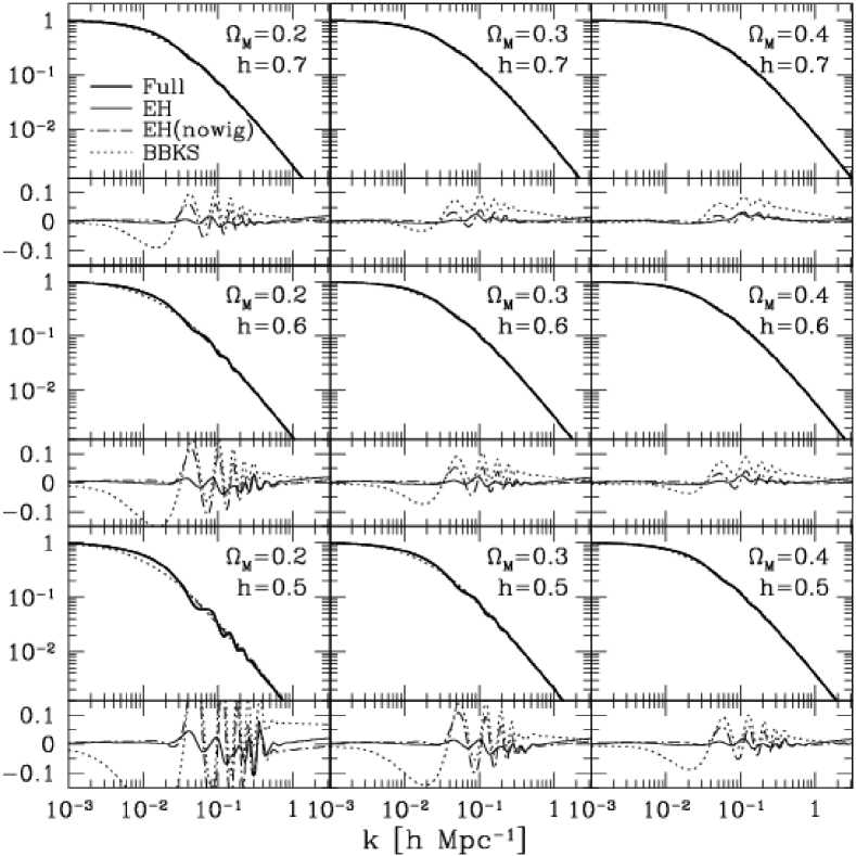
Figure 2: Comparison of transfer functions (eq. [3]) for different values of $\Omega_{M}$ and $h$ (we fix $\Omega_{b}h^{2}=0.022$). We compare transfer functions obtained from the Boltzmann equation (Full), fitting formula of Eisenstein & Hu (1998) including baryon wiggle (EH), fitting formula of Eisenstein & Hu (1998) without baryon wiggle (EH(nowig)), and fitting formula of Bardeen et al. (1986) with a shape parameter of equation (12) (BBKS). For each set of cosmological parameters, we show transfer functions (upper) and the fractional deviations from the “Full” transfer function (lower).

Although the effect of baryon can be included as a simple modification of the shape parameter, (eq. [12]), in reality including baryon yields rather complicated features in the power spectrum, such as oscillations and a sharp suppression in the transfer function below sound horizon. The fitting formula including these effects was obtained by Eisenstein & Hu (1998). In Figure 2, we compare several fitting formulae of transfer functions with direct integrals of the Boltzmann equations with CMBEASY (Doran 2003), in order to see how accurate these fitting formulae are. The amount of errors depends on adopted cosmological parameters, but around the concordance model the accuracy of the transfer function of Bardeen et al. (1986) plus equation (12) is not so good, $\lesssim 10\%$. Fitting formulae of Eisenstein & Hu (1998) are much accurate, but still contains errors of a few %. In using power spectra in research, it should be kept in mind that the approximations sometimes contain larger errors than accuracies of results.

Appendix 9.C Mass Variance

The amplitude of density fluctuations is characterized by the mass variance, $\sigma^{2}$. First we consider a density fluctuation averaged over volume $V=3M/4\pi\bar{\rho}=R_{M}^{3}$:

$$\delta\left(\vec{x},R_{M},z\right) = \int\delta\left(\vec{y},z\right)W_{M}\left(\left|\vec{x}-\vec{y}\right|;R_{M}\right)d^{3}y,$$ (14)

$$= \frac{1}{\left(2\pi\right)^{3}}\int\delta_{k}\left(z\right)\tilde{W}_{M}\left(kR_{M}\right)e^{i\vec{k}\cdot\vec{x}}d^{3}k,$$ (15)

where $W_{M}(r;R_{M})$ and $\tilde{W}_{M}(kR_{M})$ are the spatial window function and its Fourier transform, respectively. Typical choices for the window functions include

1. Top-hat:

   $$W_{M}(r;R_{M}) = \frac{3}{4\pi R_{M}^{3}}\Theta(R_{M}-r),$$ (16)

   $$\tilde{W}_{M}(kR_{M}) = \frac{3}{\left(kR_{M}\right)^{3}}\left[\sin\left(kR_{M}\right)-kR_{M}\cos\left(kR_{M}\right)\right],$$ (17)

   with $\Theta(r)$ being the Heaviside step function.

2. Gaussian:

   $$W_{M}(r;R_{M}) = \frac{1}{\left(2\pi\right)^{3/2}R_{M}^{3}}\exp\left(-\frac{r^{2}}{2R_{M}^{2}}\right),$$ (18)

   $$\tilde{W}_{M}(kR_{M}) = \exp\left(-\frac{\left(kR_{M}\right)^{2}}{2}\right).$$ (19)

Then mass variance is given by

$$\sigma_{M}(z)\equiv\sigma^{2}(R_{M},z)\equiv\langle\left|\delta\left(\vec{x},R_{M},z\right)\right|^{2}\rangle=\frac{1}{\left(2\pi\right)^{3}}\int P(k,t)\tilde{W}_{M}^{2}(kR_{M})d^{3}k.$$ (20)

In the CDM cosmology with $n_{s}=1$, its useful fitting formula is (Kitayama & Suto 1996)

$$\sigma_{M}\propto\left[1+2.208m^{p}-0.7668m^{2p}+0.7949m^{3p}\right]^{-2/9p},$$ (21)

where $p=0.0873$ and $m\equiv M(\Gamma h)^{3}/\left(\Omega_{M}h^{2}\right)/10^{12}M_{\odot}$. The above approximation and its derivative give accurate fits in the range $10^{-7}\lesssim m\lesssim 10^{5}$.

It is conventional to use $\sigma_{8}$:

$$\sigma_{8}\equiv\sigma(R_{M}=8h^{-1}{\rm Mpc},z=0),$$ (22)

as the parameter characterizing the normalization of the power spectrum. The reason for using the mass variance of $R_{M}=8h^{-1}{\rm Mpc}$ is that the observed two-point correlation function of galaxies translates to $\sigma_{8}=1$ if galaxies perfectly trace mass.

Chapter 10 Models for Dark Matter

Appendix 10.A Candidates of Cold Dark Matter

In this section, we review several specific candidates of cold dark matter.

Axion

Axions were proposed to solve the strong CP problem, i.e., large CP-violation due to degenerate vacua of $SU(3)_{\rm color}$ gauge group (Peccei & Quinn 1977). Although the mass of axions is very small, axions can be cold dark matter because they are generated non-thermally (they form a Bose-Einstein condensate) with small momentum, $\ll{\rm keV}$. The mass of axions has been constrained by making use of the coupling with photon-photon, but still axions with mass $\mu{\rm eV}\lesssim m\lesssim 1{\rm meV}$ are good candidate of cold dark matter.

Neutralino

Neutralinos are particles predicted in the framework of supersymmetry (SUSY); the SUSY scenario solves the hierarchy problem by assuming a boson partner for each fermion (and vise versa). Now it is assumed that the SUSY is broken, thus SUSY partners are much heavier than standard particles. Although “massive” sometimes means unstable, the lightest superpartners are stable because of the $R$-parity conservation which require that superpartners are produced/destroyed only in pairs. Thus the (lightest) neutralinos, which are the superpartner of neutrinos, are ideal candidate of cold dark matter.

An important implication of neutralino dark matter is that it annihilates, though the cross section is thought to be very small, $\sigma\lesssim 10^{-35}{\rm cm^{2}}$. Therefore, neutralino dark matter predicts several astrophysically interesting phenomena such as high-energy neutrinos from the Sun/Earth (e.g., Kamionkowski et al. 1995) and gamma-rays from the galactic centers (e.g., Gondolo & Silk 1999; Boehm et al. 2004).

WIMPZILLA

WIMPZILLAs are very massive relic particles produced gravitationally at the end of inflation (e.g., Chung, Kolb, & Riotto 1998). Gravitational production of particles is caused by the change of vacuum states from the inflationary (de-Sitter) phase to the matter-dominant phase. They can be cold dark matter if their mass is $\sim 10^{13}{\rm GeV}$.

Soliton

The SUSY model permits non-topological solitions, ($Q$-balls), which is stable and carry a large number of $U(1)$ charge. $Q$-balls may be stable or unstable depending on the situation, and stable $Q$-balls can be cold dark matter (Kusenko & Shaposhnikov 1998).

Appendix 10.B Alternatives to Cold Dark Matter

In this section, we review alternatives to the CDM model, which are (mainly) aimed to solve the possible problems in the CDM model at small scales (see §2). This section is partly based on the review of Ostriker & Steinhardt (2003).

Self-Interacting Dark Matter

In this model, dark matter particles have a significant self-scattering cross section comparable to the nucleon-nucleon cross section, $\sigma_{XX}/m_{X}\sim 10^{-24}{\rm cm^{2}GeV^{-1}}$ (Spergel & Steinhardt 2000). Therefore at the high-density regions (e.g., cores of dark halos), collisions between dark matter particles significantly modify the structure. Basically, collisions make the dark halos much less centrally concentrated and much rounder. In addition, collisions help to reduce the number of substructures in dark halos.

Warm Dark Matter

As shown in §9.A, warm dark matter has a larger velocity dispersion, and hence induces a cutoff in the power spectrum. Thus, while the cluster scale objects are not affected so much, it has a significant effect on small-scale structure; it lowers the number of small halos, and also makes small halos less centrally concentrated (Colín et al. 2000; Bode et al. 2001). Examples of warm dark matter are gravitinos and keV-scale sterile neutrinos.

Repulsive Dark Matter

If we consider a condensate of massive bosons interacting via a repulsive interacting potential, this results in a minimum length-scale for bound objects, and to super-fluidity. From these properties, both less central concentration and smaller substructures of galactic dark halos can be achieved (Goodman 2000).

Fuzzy Dark Matter

This model assumes that dark matter takes the form of ultra-light scalar particles ($m\sim 10^{-22}{\rm eV}$). The Compton wavelength becomes so large ($\sim$ the size of the galaxy core) that it provides soft cores and suppressed small-scale structures (Hu, Barkana, & Gruzinov 2000).

Self-Annihilating Dark Matter

Instead of self-scattering, this model considers the significant self-annihilating cross section, $\sigma/m\sim 10^{-29}{\rm cm^{2}}{\rm GeV^{-1}}$ (Kaplinghat, Knox, & Turner 2000). This annihilation removes central cusps of halos nearly independently with their mass. As an example of such model, Riotto & Tkachev (2000) considered a self-interacting Bose-field.

Fluid Dark Matter

In this mode, dark matter is regarded as a classical scalar field that interacts only with gravity and with itself. The dark matter behaves like an ideal fluid with pressure that is a function only of the mass density. This model could have effects on the core radii and on the abundance of low-mass objects (Peebles 2000).

Decaying Dark Matter

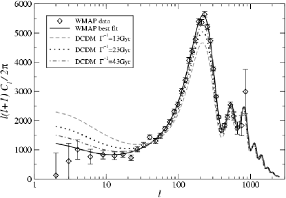
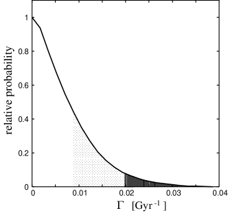
Figure 1: Left: The CMB angular power spectrum with and without decays of CDM particles. The decays basically enhance $C_{l}$ at low-$l$ through late ISW effect, and also lower first peak because of larger $\Omega_{M}h^{2}$ at early epochs. Right: The constraint on the decay rate $\Gamma$, marginalized over the other parameters. Confidence limits of 68% and 95.4% are shown by shaded regions. These Figures are taken from Ichiki, Oguri, & Takahashi (2004).

Cen (2001) proposed decaying dark matter as a solution to the possible CDM problems; if dark matter particles in dark halos decay into relativistic particles, then the central densities are lowered due to the re-expansion of halos. In addition, Ichiki et al. (2003) and Oguri et al. (2003d) showed that introducing decays of dark matter can improve the fits of observational data sets of type-Ia supernovae, mass-to-light ratios and X-ray gas fraction of clusters, and the evolution of the cluster abundance (see also Takahashi, Oguri, & Ichiki 2004a). However, it turned out that the large amount of late-time decays of dark matter is not allowed by the WMAP data; the lifetime should be $>123{\rm Gyr}$ (68% C.L.) if cold dark matter consists only of such decaying particles (Ichiki, Oguri, & Takahashi 2004, see Figure 1).

Massive Black Holes

It is possible to consider massive black holes as dark matter. Indeed, black hole dark matter may explain several observations better, such as dynamics in our galaxy (Lacey & Ostriker 1985) and anomalous flux ratios in lensed quasar systems (Mao et al. 2004). One of the powerful methods to detect such compact dark matter is gravitational lensing (e.g., Inoue & Chiba 2003). However, the observations of wide binaries seem to be inconsistent with the dark matter model consists of $M\gtrsim 50M_{\odot}$ compact objects (Yoo, Chanamé, & Gould 2004).

Chapter 11 Gravitational Lens Theory

Appendix 11.A The Lens Equation

In this section we derive the lens equation which is the fundamental equation in studying the gravitational lensing. There are many novel approaches to derive the lens equation (e.g., Schneider 1985; Schneider, Ehlers, & Falco 1992; Sasaki 1993; Seitz, Schneider, & Ehlers 1994; Futamase 1995; Surpi, Harari, & Frieman 1996). In this Appendix, we take more “intuitive” approach to derive the lens equation.

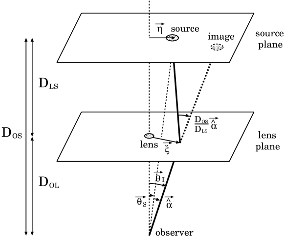
Figure 1: A schematic diagram of the lensing system. The image and source positions in each plane are denoted by $\vec{\xi}$ and $\vec{\eta}$. Angular diameter distances should be used for the distances shown in this Figure.

In most cases of strong gravitational lens studies, we can apply an approximation called thin lens approximation; that is, the light deflection takes place suddenly within a small distance. In this approximation, the deflection geometry is described in Figure 1. From the geometrical consideration, one can write down the lens equation as

$$\vec{\theta}_{\rm S}=\vec{\theta}_{\rm I}-\vec{\hat{\alpha}},$$ (1)

or equivalently

$$\frac{D_{\rm OL}}{D_{\rm OS}}\vec{\eta}=\vec{\xi}-D_{\rm OL}\vec{\hat{\alpha}}.$$ (2)

The deflection angle $\vec{\hat{\alpha}}$ can be computed as

$$\vec{\hat{\alpha}} = \frac{4G}{c^{2}}\frac{D_{\rm LS}}{D_{\rm OS}}\int d\chi\vec{\nabla}_{\perp}\phi_{\rm G}(\chi)$$ (3)

$$= \frac{1}{\pi}\int d^{2}\theta\frac{\vec{\theta}_{\rm I}-\vec{\theta}}{|\vec{\theta}_{\rm I}-\vec{\theta}|^{2}}\hat{\kappa}(D_{\rm OL}\vec{\theta}).$$

where $\phi_{\rm G}$ is the gravitational potential and $d\chi$ denotes the integral along the line of sight. We defined the dimensionless surface density as

$$\hat{\kappa}(D_{\rm OL}\vec{\theta})=\frac{\Sigma(D_{\rm OL}\vec{\theta})}{\Sigma_{\rm crit}},$$ (4)

$$\Sigma_{\rm crit}\equiv\frac{c^{2}}{4\pi G}\frac{D_{\rm OS}}{D_{\rm OL}D_{\rm LS}}.$$ (5)

Here we defined the critical surface mass density $\Sigma_{\rm crit}$.

It is useful to rewrite the above equations in a dimensionless form. We define a characteristic length $\xi_{0}$ in the lens plane and a corresponding length $\eta_{0}=\xi_{0}D_{\rm OS}/D_{\rm OL}$ in the source plane. Then we introduce the dimensionless vectors:

$$\vec{x} = \frac{\vec{\xi}}{\xi_{0}},$$ (6)

$$\vec{y} = \frac{\vec{\eta}}{\eta_{0}},$$ (7)

in each plane. With this definitions, the dimensionless lens equation becomes

$$\vec{y}=\vec{x}-\vec{\alpha}(\vec{x}),$$ (8)

$$\vec{\alpha}(\vec{x})\equiv\frac{D_{\rm OL}}{\xi_{0}}\vec{\hat{\alpha}}=\frac{1}{\pi}\int d^{2}x^{\prime}\,\kappa(\vec{x^{\prime}})\frac{\vec{x}-\vec{x^{\prime}}}{|\vec{x}-\vec{x^{\prime}}|^{2}},$$ (9)

$$\kappa(\vec{x})\equiv\hat{\kappa}(\vec{\xi})=\frac{\Sigma(\xi_{0}\vec{x})}{\Sigma_{\rm crit}}=\frac{1}{\Sigma_{\rm crit}}\int_{-\infty}^{\infty}\rho(\vec{r})\,dz.$$ (10)

In the following discussion, we mainly adopt this dimensionless lens equation (eqs. [8], [9], and [10]). If the lens object is axially symmetric, $\kappa(\vec{x})=\kappa(|\vec{x}|)$, then the lens equation reduces to the scalar equation:

$$y=x-\alpha(x),$$ (11)

$$\alpha(x)=\frac{2}{x}\int_{0}^{x}x^{\prime}\kappa(x^{\prime})dx^{\prime},$$ (12)

because $\vec{\alpha}(\vec{x})\parallel\vec{x}$.

The expression of the scaled deflection angle $\vec{\alpha}$ (eq. [9]) shows that the scaled deflection angle is a gradient of some scalar function $\psi$:

$$\vec{\alpha}(\vec{x})=\vec{\nabla}\psi(\vec{x}),$$ (13)

where

$$\psi(\vec{x})\equiv\frac{1}{\pi}\int d^{2}x^{\prime}\kappa(\vec{x}^{\prime})\ln\left|\vec{x}-\vec{x}^{\prime}\right|.$$ (14)

This is called the lens potential. From the definition (14), it is easily seen that the Laplacian of $\psi$ reduces to $2\kappa$:

$$\triangle\psi(\vec{x})=2\kappa(\vec{x}).$$ (15)

Appendix 11.B Magnification and Image Distortion

1 Magnification

Gravitational lensing changes not only the light path but also the area and shape of a light bundle. This leads to the amplification and distortion of images. Since the surface brightness $I_{\nu}$ is invariant under the gravitational deflection of light (e.g., Schneider et al. 1992), the change of flux is determined only by the change of the area of a light bundle. Thus magnification $\mu$, the ratio of flux $S_{\nu}$ with and without gravitational lensing, is simply given by

$$\mu=\frac{S_{\nu}}{S_{\nu 0}}=\frac{I_{\nu}\Delta\Omega}{I_{\nu}\Delta\Omega_{0}}=\frac{\Delta\Omega}{\Delta\Omega_{0}},$$ (16)

where the subscript $0$ means the quantities in the absence of lensing, and $\Delta\Omega$ is the solid angle of the image. Note that the magnification is independent of the frequency.

Therefore, if we define the Jacobi matrix from the lens equation,

$$A_{ij}(\vec{x})\equiv\frac{\partial y_{i}}{\partial x_{j}}=\delta_{ij}-\psi_{,x_{i}x_{j}},$$ (17)

where $\delta_{ij}$ is the Kronecker delta, $\vec{y}=(y_{1},y_{2})$, $\vec{x}=(x_{1},x_{2})$, and $\psi_{,x_{i}x_{j}}\equiv\partial^{2}\psi/\partial x_{i}\partial x_{j}$, then magnification of the image is

$$\mu(\vec{x})=\frac{1}{\det A(\vec{x})}.$$ (18)

That is, an image at $\vec{x}$ is magnified by a factor $|\mu(\vec{x})|$. The magnification factor $\mu(\vec{x})$ can take either positive or negative value, corresponding to the image with positive or negative parity (see also §11.D). The magnification factor formally diverges when $\det A(\vec{x})=0$; this point is called critical point. In many cases, a set of critical points makes one closed curve; this curve is called critical curve.

2 Convergence and Shear

Using the identity (15), we can write down the Jacobi matrix (17) as

$$A(\vec{x})=\left(\begin{array}[]{cc}1-\kappa-\gamma_{1}&-\gamma_{2}\\ -\gamma_{2}&1-\kappa+\gamma_{1}\end{array}\right),$$ (19)

where $\kappa$ is defined by equation (10), and $\gamma$ is

$$\gamma_{1} = \frac{1}{2}\left(\psi_{,x_{1}x_{1}}-\psi_{,x_{2}x_{2}}\right)$$ (20)

$$\gamma_{2} = \psi_{,x_{1}x_{2}}.$$ (21)

We note that the Jacobi matrix is the mapping which transforms the shape of the image to that of the source. This can be easily seen from

$$\delta\vec{y}=A(\vec{x})\delta\vec{x},$$ (22)

which is obtained from the perturbation of the lens equation (8).

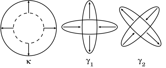
Figure 2: The schematic meaning of $\kappa$, $\gamma_{1}$, and $\gamma_{2}$ in the Jacobi matrix (19). The convergence $\kappa$ expands a light bundle, while the shear $\gamma$ changes the shape.

Figure 2 shows the meaning of each quantity in the Jacobi matrix (19). The trace part of the Jacobi matrix, $\kappa$, is called convergence. On the other hand, the traceless part, $\gamma_{1}$ and $\gamma_{2}$, is called shear.

3 Critical Curves and Caustics

The determinant of the Jacobi matrix can be calculated from equation (19) as

$$\det A=\left(1-\kappa\right)^{2}-\gamma^{2},$$ (23)

where $\gamma$ is defined by

$$\gamma=\sqrt{\gamma_{1}^{2}+\gamma_{2}^{2}}.$$ (24)

The eigenvalues of the Jacobi matrix are

$$\lambda_{\pm}=1-\kappa\pm\gamma.$$ (25)

Curves defined by $\lambda_{\pm}(\vec{x})=0$ are called the critical curves. Corresponding curves in the source plane are called caustics. As the source approaches caustics, images are highly magnified. Moreover it has been shown that the number of images changes by two if, and only if, the source crosses a caustic (e.g., Schneider et al. 1992). Therefore the caustics play a central role in the study of strong gravitational lensing. This also suggests that the multiple images must occur if $\kappa(\vec{x})>1$, or equivalently $\Sigma(\vec{\xi})>\Sigma_{\rm crit}$, for some point $\vec{x}$, because in this case the curve defined by $\lambda_{-}=0$ should exist at the outside of the point $\vec{x}$ (i.e., $\kappa(\vec{x})>1$ is a sufficient condition for multiple images).

In the case of axially symmetric lenses, eigenvectors of the Jacobi matrix point to the tangential and radial directions of the lens object. Then corresponding eigenvalues are

$$\lambda_{\rm t}(x) = 1-\kappa(x)-\gamma(x)\;\;=\;\;1-\frac{\alpha(x)}{x},$$ (26)

$$\lambda_{\rm r}(x) = 1-\kappa(x)+\gamma(x)\;\;=\;\;1-\frac{d}{dx}\alpha(x),$$ (27)

where the subscripts t and r mean tangential and radial, respectively. We also define the magnification for each direction by

$$\mu_{\rm t}(x) = \frac{1}{\lambda_{\rm t}(x)},$$ (28)

$$\mu_{\rm r}(x) = \frac{1}{\lambda_{\rm r}(x)}.$$ (29)

The magnification factor then becomes

$$\mu(x)=\mu_{\rm t}(x)\mu_{\rm r}(x).$$ (30)

The above expressions also indicate that the image near the curve $\lambda_{\rm t}=0$ ($\lambda_{\rm r}=0$) is highly elongated in the tangential (radial) direction. Thus tangential (radial) arcs are understood as the images near the critical line defined by $\lambda_{\rm t}=0$ ($\lambda_{\rm r}=0$).

Appendix 11.C Differential Time Delays

When multiple images of a single source are formed by the lens, the traveling time along the each path will, in general, be different. This fact is known as time delay (Refsdal 1964a, b, 1966), which may be ascribed to the following two effects (Cooke & Kantowski 1975). First, the curved rays are geometrically longer than straight rays, which results in a geometrical time delay $\Delta t_{\rm geom}$. Second, when the light rays travel in the gravitational field, they experience the relativistic time dilation, which results in a potential time delay $\Delta t_{\rm pot}$. Although there are many ways to derive the time delay effect (Refsdal 1966; Cooke & Kantowski 1975; Borgeest 1983; Kayser & Refsdal 1983; Schneider 1985; Schneider et al. 1992), we calculate both geometrical and potential contribution separately in order to clarify the physical meaning. Again we adopt a simple argument to derive gravitational lens time delay.

The time delay of a deflected light ray relative to an unlensed light ray is

$$c\Delta t \simeq \Delta\chi-\frac{2}{c^{2}}\int\phi_{\rm G}d\chi$$ (31)

$$\simeq (1+z_{\rm L})\Delta\ell-\frac{2(1+z_{\rm L})}{c^{2}}\int\phi d\ell$$

$$\equiv c\Delta t_{\rm geom}+c\Delta t_{\rm pot},$$

where $z_{\rm L}$ means the redshift at the lens and $\ell=\chi/(1+z_{\rm L})$ is the physical length at the lens. The above substitution holds because the deviation from the unlensed rays occurs only near the lens. Below we calculate each term in turn.

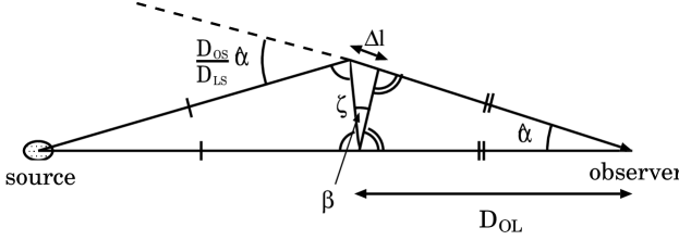
Figure 3: Calculation of the geometrical time delay. We consider the plane on which the source, observer, and deflection point (image) exist. From the purely geometrical consideration, one finds $\Delta\ell\simeq\beta\zeta$ and $\beta=D_{\rm OS}\hat{\alpha}/2D_{\rm LS}$.

• Geometrical time delay $\Delta t_{\rm geom}$
  From Figure 3, it is found

  $$\Delta\ell\simeq\beta\zeta\simeq\left(\frac{D_{\rm OS}\hat{\alpha}}{2D_{\rm LS}}\right)(D_{\rm OL}\hat{\alpha})=\frac{D_{\rm OL}D_{\rm OS}}{D_{\rm LS}}\frac{\hat{\alpha}^{2}}{2}.$$ (32)

  From the lens equation (8), $\hat{\alpha}$ is written as

  $$\hat{\alpha}^{2}=\frac{\xi_{0}^{2}}{D_{\rm OL}^{2}}(\vec{x}-\vec{y})^{2}.$$ (33)

  Then the geometrical time delay $\Delta t_{\rm geom}$ becomes

  $$c\Delta t_{\rm geom}=\frac{\xi_{0}^{2}D_{\rm OS}}{D_{\rm OL}D_{\rm LS}}(1+z_{\rm L})\frac{(\vec{x}-\vec{y})^{2}}{2}.$$ (34)

• Potential time delay $\Delta t_{\rm pot}$
  The potential time delay is obtained by performing the integral:

  $$c\Delta t_{\rm pot} = -\frac{2(1+z_{\rm L})}{c^{2}}\int\phi_{\rm G}d\ell$$ (35)

  $$\simeq -\frac{4G(1+z_{\rm L})}{c^{2}}\int d^{2}\xi^{\prime}\Sigma(\vec{\xi^{\prime}})\ln\frac{|\vec{\xi}-\vec{\xi}^{\prime}|}{\xi_{0}}$$

  $$= -\frac{\xi_{0}^{2}D_{\rm OS}}{D_{\rm OL}D_{\rm LS}}(1+z_{\rm L})\psi(\vec{x}).$$

What we observe is the total time delay, not individual terms. The total time delay of a deflected light ray $\Delta t$ is derived simply by summing up these two effects:

$$c\Delta t = c\Delta t_{\rm geom}+c\Delta t_{\rm pot}$$ (36)

$$= \frac{\xi_{0}^{2}D_{\rm OS}}{D_{\rm OL}D_{\rm LS}}(1+z_{\rm L})\phi(\vec{x},\vec{y}),$$

where we defined the Fermat potential:

$$\phi(\vec{x},\vec{y})\equiv\frac{(\vec{x}-\vec{y})^{2}}{2}-\psi(\vec{x}).$$ (37)

The Fermat potential has several interesting properties. For example, the lens equation (8) is rewritten in terms of the Fermat potential:

$$\vec{\nabla}\phi(\vec{x},\vec{y})=0.$$ (38)

This means that the lensed images are formed at the points where the Fermat potential is stationary. This is certainly Fermat’s principle in geometrical optics, which says that the actual light trajectory is such that the light-travel time is stationary on it under the first order variations.

Since the time delay is, in practice, observed between two images produced from one source, we write this as

$$c\Delta t(\vec{y})=\frac{\xi_{0}^{2}D_{\rm OS}}{D_{\rm OL}D_{\rm LS}}(1+z_{\rm L})\left[\phi(\vec{x}^{(1)},\vec{y})-\phi(\vec{x}^{(2)},\vec{y})\right],$$ (39)

where $\vec{x}^{(i)}$, $i=1,2$, are two image positions, produced by a source at $\vec{y}$.

Appendix 11.D Mathematical Aspects

In this section, we briefly review some mathematical aspects of strong gravitational lensing, which may be useful to understand image position/magnification patterns in strong lens systems. Basically we follow the discussion of Schneider et al. (1992); please refer it for more comprehensive discussions.

1 Classification of Images

It has been shown in the previous section that lensed images are formed at the points where the derivative of the Fermat potential $\phi$ (eq. [37]) vanishes. Thus images are located at local minima and saddle points of the constant Fermat potential surface (i.e., the arrival time surface). The properties of such stationary point is characterized by the second derivative of the Fermat potential, i.e., the Jacobi matrix (eq. [17]). Specifically, images are classified into the following three types:

• Type I: Minimum of $\phi$, defined by ${\rm det}A>0$ and ${\rm tr}A>0$.

• Type II: Saddle point of $\phi$, defined by ${\rm det}A<0$.

• Type III: Maximum of $\phi$, defined by ${\rm det}A>0$ and ${\rm tr}A<0$.

Since the magnification factor is $\mu=({\rm det}A)^{-1}$, it is said that images of types I and III have positive parities, while images of type II have negative parity.

We denote the number of images of each type as $n_{\rm I}$, etc. The total number of images is denoted by $n=n_{\rm I}+n_{\rm II}+n_{\rm III}$. We consider a single, thin lens system whose surface mass density $\kappa(\vec{x})$ is smooth and decrease faster than $|\vec{x}|^{-2}$ at $|\vec{x}|\rightarrow\infty$. The deflection angle $\vec{\alpha}(\vec{x})$ is continuous, bounded ($|\vec{\alpha}(\vec{x})|\leq a$), and $|\vec{\alpha}(\vec{x})|\rightarrow 0$ for both $|\vec{x}|\rightarrow 0$ and $\infty$. Then, the following theorems are proven:

Theorem 1

The numbers of lenses satisfy the following relations: (a) $n_{\rm I}\geq 1$, (b) $n<\infty$, (c) $n=n_{\rm I}=1$ for sufficiently large $\vec{y}$.

Sketch of proof. (a) The Fermat potential $\phi$ must have the global minimum, which corresponds to an image of type I. (b) The boundness implies the images must be contained in the disc $|\vec{x}|\leq|\vec{y}|+a$, for a fixed $\vec{y}$. Since images are isolated by assumption, $n<\infty$. (c) For $|\vec{x}|\rightarrow\infty$, $A\rightarrow I$, and thus a circle of radius $R$, outside of which there is only one image of type I, exists. Again, the boundness implies $|\vec{x}|\geq|\vec{y}|-a>R$ if we choose $|\vec{y}|>a+R$. Combining these results yields $n=n_{\rm I}=1$. $\blacksquare$

To prove another theorem on the number of lenses, we need the index theorem. First, we need to define the index.

Definition. Let $S$ be a surface $S$, and let $\vec{V}$ be a tangent vector field on $S$. For each point $p$ of $S$, the index, denoted as $I(p)$, is defined by

$$I(p)=\frac{1}{2\pi}\oint_{c_{\epsilon}}d\varphi,$$ (40)

where $\vec{V}=|\vec{V}|(\cos\varphi,\sin\varphi)$, and $c_{\epsilon}$ is an oriented, closed curve enclosing the point $p$

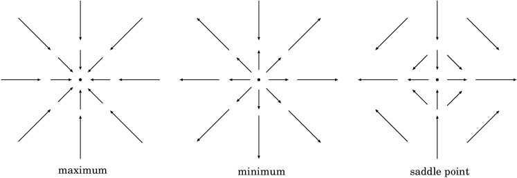
Figure 4: Vector fields around three stationary point of $\phi$.

Note that the index of a non-critical point $\vec{V}(p)\neq 0$ is $0$, and only critical points have non-vanishing index. In our specific example, these points correspond to maxima, minima, and saddle points of the Fermat potential $\phi$. Figure 4 shows the vector fields $\vec{\nabla}\phi$ around these critical points; by inspection, we find that the index of an extremum (i.e., maximum or minimum) is $+1$, and that of a saddle point is $-1$.

Theorem 2 (Poincaré-Hopf index theorem)

Let $\vec{V}$ be a continuous tangent vector filed with isolated singularities on the compact, connected, orientable 2-dimensional surface $S$. If we denote critical points by $p_{i}$,

$$\sum I(p_{i})=\chi(S),$$ (41)

where $\chi(S)$ is the Euler characteristic of $S$.

The Euler characteristic is a topological invariant, and for polyhedron it is defined by $V-E+F$, where $V$, $E$, and $F$ are the numbers of vertices, edges, and faces, respectively. For instance, the Euler characteristic of $S^{2}$ is 2. Then we obtain the following theorem:

Theorem 3

The numbers of images satisfy the following relation: $n_{\rm I}+n_{\rm III}=1+n_{\rm II}$.

Sketch of proof. By considering the standard stereographic projection, we obtain $\mathbb{R}^{2}\approx S^{2}-\{\rm N\}$, where N is the sphere’s north pole. The north pole corresponds to the infinity, and the index of the point is $+1$ because the vector filed $\vec{\nabla}\phi$ is asymptotically radial. Then, the index theorem gives $n_{\rm I}-n_{\rm II}+n_{\rm III}=1$. $\blacksquare$

The above theorem implies the number of images is odd, the number of even-parity images exceeds that of odd parity images by one (Burke 1981), $n_{\rm II}\geq n_{\rm III}$, and $n>1$ if and only if $n_{\rm II}\geq 1$.

Theorem 4

The image of a source that arrives first at the observer is of type I and appears brighter than the source would appear in the absence of the lens.

Sketch of proof. The global minimum of the Fermat potential $\phi$ corresponds to an image of type I, and by definition, it arrives first. The condition of type I is ${\rm tr}A>0$, i.e., $\kappa<1$. This implies

$$\mu^{-1}=(1-\kappa)^{2}-\gamma^{2}<1-\gamma^{2}\leq 1,$$ (42)

therefore we obtain $\mu>1$ (Schneider 1984). $\blacksquare$

Finally, we comment on the odd-number theorem. In most lensed quasar systems, the number of images are even (mostly 2 or 4; see Kochanek et al. 2004b). This implies either the central mass distribution is so cuspy that the assumption of $|\vec{\alpha}(\vec{x})|\rightarrow 0$ for $|\vec{x}|\rightarrow 0$ becomes wrong (i.e., steeper than $\rho(r)\propto r^{-2}$) or the central image is demagnified enough not to be observed. Since the amount of demagnification depends on the central mass distribution of the lens so that the steeper density profile tends to demagnify the central image more, the absence/detection of the central image is used to constrain the mass distribution in the innermost region of the lens (e.g., Rusin & Ma 2001a; Keeton 2003a; Winn, Rusin, & Kochanek 2004).

2 Fold and Cusp Caustics

Hereafter we denote $\phi_{i}\equiv(\vec{\nabla}\phi)_{i}$, etc. In this notation, the lens equation is

$$\phi_{i}=0.$$ (43)

As discussed in §3, critical curves and caustics are defined by

$$D\equiv{\rm det}\,\phi_{ij}=0.$$ (44)

We consider images around a critical point $\vec{x}^{(0)}$. Suppose that $A^{(0)}$ has rank 1 and $\vec{\nabla}D\neq 0$. Then we can introduce the coordinate system around $\vec{x}^{(0)}$ so that $A^{(0)}$ is diagonal with $A_{11}^{(0)}\neq 0$ and $A_{22}^{(0)}$. Since

$$D=\phi_{11}\phi_{22}-\phi_{12}^{2},$$ (45)

the normal vector and tangential vector at $\vec{x}^{(0)}$ become

$$\vec{N}^{(0)}=\vec{\nabla}D=\phi_{11}^{(0)}(\phi^{(0)}_{221},\phi^{(0)}_{222}),$$ (46)

$$\vec{T}^{(0)}=R(\pi/2)\vec{\nabla}D=\phi_{11}^{(0)}(-\phi^{(0)}_{222},\phi^{(0)}_{221}).$$ (47)

Thus we consider the following two cases:

• Fold: $A^{(0)}\cdot\vec{T}^{(0)}\neq 0$
  In this case, the Taylor expansion of the Fermat potential $\phi$ becomes

  $$\phi=\phi^{(0)}+\frac{1}{2}y^{2}-\vec{x}\cdot\vec{y}+\frac{1}{2}\phi_{11}^{(0)}x_{1}^{2}+\frac{1}{2}\phi_{112}^{(0)}x_{1}^{2}x_{2}+\frac{1}{2}\phi_{122}^{(0)}x_{1}x_{2}^{2}+\frac{1}{6}\phi_{222}^{(0)}x_{2}^{3}.$$ (48)

  Then the lens equation is

  $$y_{1} = \phi_{11}^{(0)}x_{1}+\phi_{112}^{(0)}x_{1}x_{2}+\frac{1}{2}\phi_{122}^{(0)}x_{2}^{2},$$ (49)

  $$y_{2} = \frac{1}{2}\phi_{112}^{(0)}x_{1}^{2}+\phi_{122}^{(0)}x_{1}x_{2}+\frac{1}{2}\phi_{222}^{(0)}x_{2}^{2}.$$ (50)

  Then it is straightforward to compute the critical curve and caustic:

  Critical curve: $$\displaystyle{\phi_{122}^{(0)}x_{1}+\phi_{222}^{(0)}x_{2}=0,}$$ (51)

  Caustic: $$\displaystyle{Q\equiv 2\left(\phi_{11}^{(0)}\right)^{2}\phi_{222}^{(0)}y_{2}-\left[\phi_{112}^{(0)}\phi_{222}^{(0)}-\left(\phi_{122}^{(0)}\right)^{2}\right]y_{1}^{2}=0.}$$ (52)

  From this, images near the critical curve are derived as

  $$x_{1} = \frac{\phi_{222}^{(0)}y_{1}-\phi_{122}^{(0)}y_{2}}{\phi_{11}^{(0)}\phi_{222}^{(0)}},$$ (53)

  $$x_{2} = \frac{-\phi_{122}^{(0)}y_{1}\pm\sqrt{Q}}{\phi_{11}^{(0)}\phi_{222}^{(0)}}.$$ (54)

  Thus we have two images around a fold caustic.

• Cusp: $A^{(0)}\cdot\vec{T}^{(0)}=0$
  As in the case of fold caustic, the Taylor expansion of the Fermat potential $\phi$ becomes

  $$\phi=\phi^{(0)}+\frac{1}{2}y^{2}-\vec{x}\cdot\vec{y}+\frac{1}{2}\phi_{11}^{(0)}x_{1}^{2}+\frac{1}{2}\phi_{112}^{(0)}x_{1}^{2}x_{2}+\frac{1}{2}\phi_{122}^{(0)}x_{1}x_{2}^{2}+\frac{1}{24}\phi_{2222}^{(0)}x_{2}^{4}.$$ (55)

  Then the lens equation is

  $$y_{1} = \phi_{11}^{(0)}x_{1}+\phi_{112}^{(0)}x_{1}x_{2}+\frac{1}{2}\phi_{122}^{(0)}x_{2}^{2},$$ (56)

  $$y_{2} = \frac{1}{2}\phi_{112}^{(0)}x_{1}^{2}+\phi_{122}^{(0)}x_{1}x_{2}+\frac{1}{6}\phi_{2222}^{(0)}x_{2}^{3}.$$ (57)

  Again it is straightforward to compute the critical curve and caustic:

  Critical curve: $$\displaystyle{2\phi_{122}^{(0)}\phi_{11}^{(0)}x_{1}+\left[\phi_{2222}^{(0)}\phi_{11}^{(0)}-2\left(\phi_{122}^{(0)}\right)^{2}\right]x_{2}^{2}=0,}$$ (58)

  Caustic: $$\displaystyle{8\left(\phi_{122}^{(0)}\right)^{3}y_{1}^{3}+9\left(\phi_{11}^{(0)}\right)^{2}\left[\phi_{2222}^{(0)}\phi_{11}^{(0)}-3\left(\phi_{122}^{(0)}\right)^{2}\right]y_{2}^{2}=0.}$$ (59)

  That is, the caustic is a semicubic parabora. From this, it is found that the images near the critical curve are given by the solution of the following equations:

  $$x_{1}-\frac{y_{1}}{\phi_{11}^{(0)}}+\frac{\phi_{122}^{(0)}}{2\phi_{11}^{(0)}}x_{2}^{2}=0,$$ (60)

  $$x_{2}^{3}+\frac{6\phi_{122}^{(0)}y_{1}}{\phi_{2222}^{(0)}\phi_{11}^{(0)}-3\left(\phi_{122}^{(0)}\right)^{2}}x_{2}-\frac{6\phi_{11}^{(0)}y_{2}}{\phi_{2222}^{(0)}\phi_{11}^{(0)}-3\left(\phi_{122}^{(0)}\right)^{2}}=0.$$ (61)

  Thus we have three images around a cusp caustic.

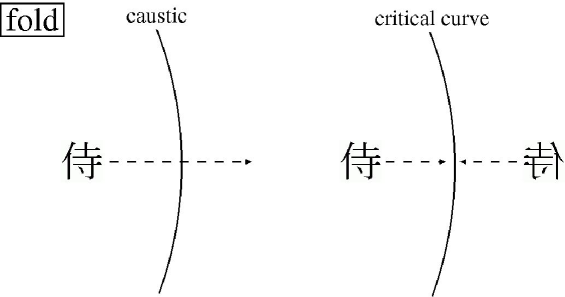
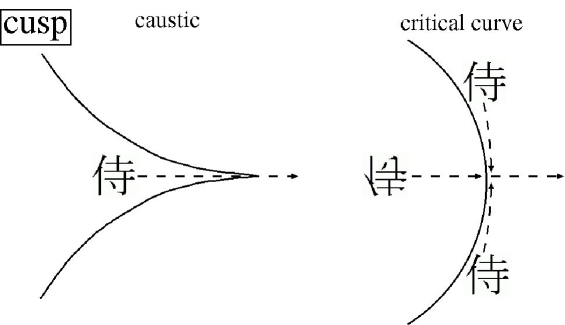
Figure 5: Images around fold (upper) and cusp (lower) caustics. As a source moves from inside to outside the fold caustics, two images merge and vanish. On the other hand, at the cusp caustic three images merge and one image remains. In this Figure, the left hand side corresponds to the center of mass distribution. We choose a complicated character (samurai in Japanese) as a source, in order to explicitly show parities of images.

Figure 5 shows images around fold and cusp caustics. As crossing fold caustics, two images with different parities are newly created/destroyed. On the other hand, as crossing from outside to inside cusp caustics, one image is split into three images.

Chapter 12 Simulations for Arcs

Most of this method presented in this Appendix follows the work by Miralda-Escudé (1993b), Bartelmann & Weiss (1994), and Oguri (2002b).

Appendix 12.A Lens Mapping

To begin with, we choose a sufficiently large region in the lens plane in which all the arcs are exist. In this region we prepare regular grids. Each grid point is denoted by $(x_{1i},x_{2j})$, where integers $i$ and $j$ are restricted in $1\leq i,j\leq N_{\rm grid}$. In the practical calculations, we adopt $N_{\rm grid}=2048$ throughout the thesis. Given the deflection angle $\vec{\alpha}$, we can calculate the source point $(y_{1}(i,j),y_{2}(i,j))$ which corresponds to $(x_{1i},x_{2j})$ by using the lens equation. We calculate this for all grid points and this yields “mapping table”.

Next we consider the source with center $(y_{\rm 1c},y_{\rm 2c})$ and (dimensionless) radius $r_{\rm S}$ and ellipticity $e_{\rm S}$. We regard the grid point $(x_{1i},x_{2j})$ is a part of lensed images if the following condition is satisfied:

$$\frac{\left[y_{1}(i,j)-y_{\rm 1c}\right]^{2}}{r_{\rm S}^{2}/(1-e_{\rm S})}+\frac{\left[y_{2}(i,j)-y_{\rm 2c}\right]^{2}}{r_{\rm S}^{2}(1-e_{\rm S})}\leq 1.$$ (1)

For all the grids we check this condition and obtain the pattern of lensed images. In general, multiple images can be generated by gravitational lensing. Thus we search each “image” grid and recognize neighboring “image” grids as the same image. The magnification of the image is then proportional to the number of grid points it contains. We show a schematic diagram of the method in Figure 1.

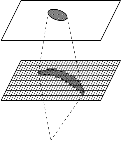
Figure 1: Schematic diagram of the lens mapping algorithm. We prepare the regular grid in the lens (image) plane, and each grid is checked whether it belongs to the source when mapped into the source plane.

Appendix 12.B Recognition of Arcs

To analyze the lens properties, we calculate the magnification $\mu$, length $l$, and width $w$ of the image. For the multiply lensed system, we calculate above quantities for each image.

• Magnification $\mu$
  Magnification $\mu$ is easily calculated from the number of grid points $N_{\rm image}$ which are recognized as the image:

  $$\mu=\frac{N_{\rm image}(\Delta x)^{2}}{\pi r_{\rm S}^{2}},$$ (2)

  where $\Delta x$ is the size of the grid. This gives fairly accurate values because images contains many grid points in our calculations; typically $N_{\rm image}\gtrsim 50$.

• Length $l$
  First we search the center of the image (point C) as the point at which the value of the left hand side in equation (1) becomes the smallest. Then we find the point A in the image which is the farthest away from the center. Then we find the point B, also along the image, which is the farthest away from the point A. We calculate the length of the image by $l={\rm\overline{AC}+\overline{BC}}$.

• Width $w$
  The width is taken such that $\pi lw=\mu\pi r_{\rm S}^{2}$.

Then, the axis ratio of the arc is defined by

$$\epsilon=\frac{l}{w},$$ (3)

and this quantity plays a central role in arc statistics (see Chapter 4).

Chapter 13 The Sloan Digital Sky Survey

Appendix 13.A Introduction

The Sloan Digital Sky Survey (SDSS) is the most ambitious astronomical survey project ever undertaken. The survey will conduct in both photometric and spectroscopic surveys of $\sim 10,000{\rm deg^{2}}$ ($1/4$) of the entire sky, using a dedicated wide-field 2.5-meter telescope at Apache Point Observatory (APO), New Mexico, USA. The SDSS will determine the positions, redshifts, and absolute magnitudes of $\sim 10^{6}$ galaxies and $\sim 10^{5}$ quasars. The main purpose of the SDSS is to map the 3-dimensional large-scale structure in the universe.

The striking advantage of the SDSS is the homogeneity of the survey, despite it covers very large area of the sky. The SDSS will have a significant impact on astronomical studies as diverse as the large-scale structure of the universe, the origin and evolution of galaxies, the relation between dark and luminous matter, the structure of our own Milky Way, and the properties and distribution of the dust from which stars like our sun were created.

The SDSS started the survey in 2000, and is now ongoing; the SDSS will be completed in 2005. So far the SDSS data release have been done three times (Stoughton et al. 2002; Abazajian et al. 2003, 2004), and all the data will be publicly available till the middle of 2006 (see Table 1 and Figure 1). Once completed, the SDSS will become one of the most fundamental archives for optical astronomy for next decades.

Data Release	Baseline Schedulea	Actual/Forecastb	Photometry[deg2]c	Spectroscopy[deg2]c
EDR	July 2001	5-Jun-2001	462	386
DR1	Jan 2003	4-Apr-2003	2,099	1,360
DR2	Jan 2004	15-Mar-2004	3,324	2,627
DR3	Oct 2004	Oct 2004	5,300	4,600
DR4	July 2005	July 2005	6,500	5,800
Finald	July 2006	July 2006	7,700	7,000

Table 1: The SDSS data release schedule for the 5-year baseline survey. This Table is taken from a webpage at http://www.sdss.org/science/DRschedule.html.
      ^a Baseline schedule as presented in: Data Distribution to the Astronomy Community, Revision 1, September 8, 2000.            
      ^b Dates for the EDR, DR1, and DR2 are actual release dates; dates for releases after April 2004 are current forecasts.                                                                            
      ^c The data volumes shown for EDR, DR1, and DR2 are the actual volumes released; data volumes for DR3, DR4 and the final release are estimates based on current forecasts.                                                                            
      ^d The final data release corresponds to the release of the last increment of processed data.

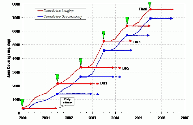
Figure 1: The SDSS data release schedule for the 5-year baseline survey. The green markers correspond to the date of acquiring the last imaging data that will be included in a particular release. Spectroscopic data is based on imaging data in the data set and may have been obtained at a later date. Observations that are part of the five-year baseline survey are scheduled to end in July 2005. This Figure is taken from a webpage at http://www.sdss.org/science/DRschedule.html.

Appendix 13.B Telescope, Camera, and Spectrograph

The SDSS observing site is at APO in New Mexico, USA. The site is about 2,840-meter above sea level. The SDSS has two telescope; the SDSS main telescope and the photometric telescope.

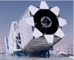
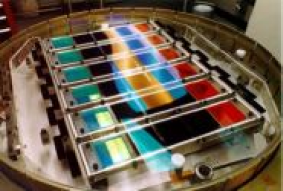
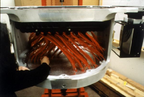
Figure 2: Left: The SDSS 2.5-meter main telescope at Apache Point Observatory. Center: The SDSS camera assembly. There are 20 photometric and 24 astrometric/focus CCDs. Right: A plug plate that has been drilled, fitted with optical fibers, and mounted on the spectrograph assembly. These Figure are taken from a webpage at http://www.sdss.org/.

The SDSS main telescope has a primary mirror with a diameter of 2.5-meter, and has a $3^{\circ}$ diameter field of view (Figure 2 Left). The remarkably wide-angle view is to create a map of the sky, and is realized by the improved Ritchey-Chrétien design. The imaging camera (Figure 2 Center) is set on the focal plane; it consists of a $5\times 6$ (i.e., 6 chips for each broad band) large CCD chips ($2048\times 2048$ pixels) for the photometric observations and 24 CCDs ($2048\times 400$ pixels) for the astrometry/focusing (Gunn et al. 1998). The scale of the pixel is $0\farcs 4{\rm pisel^{-1}}$, about $1/4$ of the typical seeing size in observations at APO. The SDSS photometric system uses five broad band, $ugriz$ (Fukugita et al. 1996); the SDSS filter response curves are shown in Figure 3.

The photometric telescope has a primary mirror with a diameter of 0.5-meter, is outfitted with a CCD ($2048\times 2048$ pixels), and has a $1,600{\rm arcmin}^{2}$ field of view. The photometric telescope is aimed to observe the secondary standard stars for the photometric calibration. The secondary standard star network used here (Smith et al. 2002) covers the whole area of the region the SDSS observes.

The spectroscopic observations are conducted by the double spectrograph with a dichroic splitter and $2048\times 2048$ CCD chips, by setting a plate fitted with 320 fibers on the focal plane (Figure 2 Right). In reality, two identical instruments fed by a single plug-plate are used to obtain 640 spectra per exposure. The photons come from a fiber are divided into blue (3800Å–6100Å) and red (5900Å–9200Å) by dichronic splitter. They are sent to the grisms; each grating is 640 line mm^-1 (blue) and 440 line mm^-1 (red). The spectral resolution is $\lambda/\Delta\lambda=1800$. Since each fiber has a diameter of 3-mm on the plate, it is impossible to observed a pair of objects whose separation is $\leq 55^{\prime\prime}$ in a single plate. Thus the SDSS adopts the adaptive tiling method to allocate fibers to spectroscopic targets, and achieves a sampling rate of $\geq 92\%$ for all targets (Blanton et al. 2003).

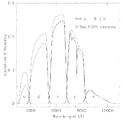
Figure 3: The SDSS filter response curves for $u^{\prime}$, $g^{\prime}$, $r^{\prime}$, $i^{\prime}$, and $z^{\prime}$, without (upper curves) and with (lower curves) the atmospheric extinction. This Figure is taken from Stoughton et al. (2002).

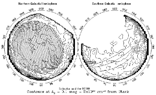
Figure 4: The footprints of the Northern and Southern SDSS surveys. The tracks for the photometric survey are shown by heavy lines. The contours show the extinction measured from the HI column density. This Figure is take from a webpage at http://archive.stsci.edu/sdss/index.html.

Appendix 13.C Observations and Data Reductions

Since the SDSS needs to observe the enormous sky area, it adopts the time delay and integrated mode (or scanning mode); the telescope is fixed during the observations, and the observing fields are changing as the earth rotate. In this case, the size of a CCD chip ($13\farcm 52$) determines the exposure time, $55$ sec. The advantages of this mode include (i) it results in almost 100% observing efficiency because we can save the readout time. (ii) it reduces the flat-fielding problem from 2-dimension to 1-dimension. At the same time, the astrometric CCDs and photometric telescope observe the standard stars for calibrations. The astrometric CCDs allow us to determine positions of sources brighter than $r=20.5$ with accuracy better than $0\farcs 1$ (Pier et al. 2003).

Because of gaps between CCD cameras, one needs a slightly shifted drift scan observations to fill the gaps. Thus a “stripe” consists of two runs. Although the SDSS mainly observes the north galactic hemisphere, in addition it observes a small region on the south galactic hemisphere. The survey region is determined so that the region has minimum galactic extinction and minimum atmospheric extinction. Figure 4 shows the survey regions and the extinction.

Targets of spectroscopic observations are chosen according to target selection algorithms (see below). As seen in Figure 2 Right, 640 fibers are plugged for positions of targeted objects on each plate . Spectra are usually obtained with $3\times 15$ minutes exposures, but it may be changed according to the observing conditions.

The SDSS automated data processing, called pipeline, is used to reduce the data, to select spectroscopic targets, and to make a object catalog. There are three main pipelines; photometric pipeline, target selection pipeline, and spectroscopic pipeline.

The photometric pipeline reduces the photometric data and make a object catalog. It carries out bias subtraction, flat-fielding, and fixing bad pixels/columns. The data of the photometric telescope are also reduced automatically; the pipeline measures the extinction coefficients and photometric parameters in real time (Hogg et al. 2001). Then it searches objects in the data with templates of stars and galaxies, and calculates several values such as magnitudes, colors, object-types, etc. The data are put into a catalog named “tsObj”.

After making the object catalog, the target selection pipelines select the object for the spectroscopic observations. The target selection algorithms have been developed for galaxies (Strauss et al. 2002), luminous red galaxies (Eisenstein et al. 2001), quasars (Richards et al. 2002), etc. These target selection algorithms are determined so that the resulting spectroscopic samples become approximately homogeneous.

Finally, the spectroscopic pipeline reduces the data and obtains 1-dimensional spectra. It also identifies emission/absorption lines, obtains accurate radial velocities, and classifies the spectra.

Chapter 14 Mass Modeling of SDSS J1004+4112

Appendix 14.A One-component Models

To search for mass models that can explain the image configuration of the large-separation lensed quasar SDSS J1004+4112 (Chapter 6), we use standard lens modeling techniques as implemented in the software of Keeton (2001d). The main constraints come from the image positions. We also use the flux ratios as constraints, although we broaden the errorbars to 20% to account for possible systematic effects due to source variability and time delays, micro- or milli-lensing, or differential extinction (See Table 1 for the full set of constraint data). In particular, the different colors of the images and the different absorption features seen in Figure 4 suggest that differential extinction may be a significant effect. Here we do not use the position of the main galaxy as a constraint, because we want to understand what constraints can be placed on the center of the lens potential from the lens data alone.

We first consider the simplest possible models for a 4-image lens: an isothermal lens galaxy with a quadrapole produced either by ellipticity in the galaxy or by an external shear. A spherical isothermal lens galaxy has surface mass density

$$\kappa(r)=\frac{\Sigma(r)}{\Sigma_{\rm crit}}=\frac{r_{\rm ein}}{2r}\ ,$$ (1)

where $r_{\rm ein}$ is the Einstein radius of the lens, and $\Sigma_{\rm crit}$ is the critical surface mass density (eq. [5]). The Einstein radius is related to the velocity dispersion $\sigma$ of the galaxy by

$$r_{\rm ein}=4\pi\,\left(\frac{\sigma}{c}\right)^{2}\,\frac{D_{\rm LS}}{D_{\rm OS}}\ .$$ (2)

For an elliptical model we replace $r$ with $r[1+((1-q^{2})/(1+q^{2}))\cos 2(\theta-\theta_{e})]^{1/2}$ in the surface density, where $q$ and $\theta_{e}$ are the axis ratio and position angle of the ellipse.

Simple models using either pure ellipticity or pure shear fail miserably, yielding $\chi^{2}$ values no better than $2\times 10^{4}$ for $N_{\rm dof}=4$ degrees of freedom. This failure is not surprising: most 4-image lenses require both ellipticity and external shear (e.g., Keeton, Kochanek, & Seljak 1997), and such a situation is likely in SDSS J1004+4112 since the main galaxy is observed to be elongated and the surrounding cluster surely contributes a shear.

Object	$x$[arcsec]a	$y$[arcsec]a	Flux[arbitrary]b	PA[deg]c
A	$0.000\pm 0.012$	$0.000\pm 0.012$	$1.0\pm 0.2$	$\cdots$
B	$-1.301\pm 0.011$	$3.500\pm 0.011$	$0.682\pm 0.136$	$\cdots$
C	$10.961\pm 0.012$	$-4.466\pm 0.012$	$0.416\pm 0.083$	$\cdots$
D	$8.329\pm 0.007$	$9.668\pm 0.007$	$0.195\pm 0.039$	$\cdots$
G1	$7.047\pm 0.053$	$4.374\pm 0.053$	$\cdots$	$-19.9$

Table 1: Summary of positions, flux ratios, and position angles (PA) of SDSS J1004+4112 used in the mass modeling.                                                            
      ^a The positive directions of $x$ and $y$ are defined by West and North, respectively.                                                                           
      ^b Errors are broadened to 20% to account for possible systematic effects.                                                                           
      ^c Degrees measured East of North.

Figure 1: Critical curve (left) and caustic (right) for the best-fit SIE+shear lens model of SDSS J1004+4112. In the left panel, the filled circles mark the image positions, the open circle indicates the observed position of the brightest cluster galaxy G1, and the cross marks the best-fit deflector position. In the right panel the filled circle marks the inferred source position.

Figure 2: Likelihood contours drawn at 1$\sigma$, 2$\sigma$, and 3$\sigma$ for various parameter combinations in SIE+shear lens models. The left panel shows constraints on the position of the deflector; the circle marks the observed position of the main galaxy. The right panel shows contours in the ellipticity–external shear plane.

We therefore try models consisting of a singular isothermal ellipsoid (SIE) plus an external shear $\gamma$. Even though such models are still comparatively simple, they can fit the data very well with a best-fit value of $\chi^{2}=0.33$ for $N_{\rm dof}=2$. The best-fit model has an Einstein radius $r_{\rm ein}=6\farcs 9=35\,h^{-1}$ kpc corresponding to a velocity dispersion of 700 km s^-1, an ellipticity $e=0.50$ at position angle $\theta_{e}=21\fdg 4$, and an external shear $\gamma=0.25$ at position angle $\theta_{\gamma}=-60\fdg 9$. Among other known lenses, such a large shear is found only in lenses lying in cluster environments (Burud et al. 1998; Barkana et al. 1999). Figure 1 shows the critical curves and caustics for the best-fit model. The inferred source position lies very close to the caustic and fairly near a cusp, implying that the total magnification is $\sim$57. Figure 2 shows the allowed ranges for the position of the deflector and the ellipticity and external shear in the model. The models indicate a small but significant offset of $1\farcs 6=7.9\,h^{-1}$ kpc between the center of the lens potential and the main galaxy, although it remains to be seen whether that offset is real or an artifact of these still simple lens models.

Appendix 14.B Two-component Models

Even though the simple SIE+shear model provides a good fit to the data, we believe that it is not physically plausible because the system clearly has multiple mass components and it seems unlikely that all of the mass is associated with a single $\sim$700 km s^-1 isothermal component. The next level of complication is to add a mass component representing the cluster halo. We still model the galaxy G1 explicitly, treating it as an isothermal ellipsoid constrained by its observed position. At this point we do not further complicate the model by attempting to treat the other galaxies within the lens explicitly.

1 Methods

We model the cluster component with an NFW profile which has been predicted in cosmological $N$-body simulations:

$$\rho(r)=\frac{\rho_{\rm crit}(z)\delta_{\rm c}(z)}{\left(r/r_{\rm s}\right)\left(1+r/r_{\rm s}\right)^{2}},$$ (3)

where $r_{\rm s}$ is a scale radius, $\delta_{\rm c}$ is a characteristic overdensity (which depends on redshift), and $\rho_{\rm crit}(z)$ is the critical density of the universe. Although the NFW density profile appears to deviate from the results of more recent $N$-body simulations in the innermost region, we adopt this form for simplicity. The lensing properties of a spherical NFW halo are described by the lens potential (Bartelmann 1996; Golse et al. 2002; Meneghetti et al. 2003a)

$$\psi(r)=2\kappa_{\rm s}\,r_{\rm s}^{2}\left[\ln^{2}\frac{r}{2r_{\rm s}}-\mbox{arctanh}^{2}\sqrt{1-(r/r_{\rm s})^{2}}\right],$$ (4)

where the lensing strength is specified by the parameter $\kappa_{\rm s}=b_{\rm NFW}/4$ (see eq. [15]). Since asphericity in the cluster potential is important in modeling this system, we generalize the spherical model by adopting elliptical symmetry in the potential. Making the potential (rather than the density) elliptical makes it possible to compute the lensing properties of an NFW halo analytically (Golse et al. 2002; Meneghetti et al. 2003a). We may still be over-simplifying the mass model, because the cluster profile may have been modified from the NFW form by baryonic processes such as gas cooling (Rees & Ostriker 1977; Blumenthal et al. 1986), and the cluster may have a complex angular structure if it is not relaxed (e.g., Meneghetti et al. 2003a). To allow for the latter possibility, we still include a tidal shear in the lens model that can approximate the effects of complex structure in the outer parts of the cluster. Overall, our goal is not to model all of the complexities of the lens potential, but to make the minimal realistic model and see what we can learn.

Even with our simplifying assumptions, we still have a complex parameter space with 11 parameters defining the lens potential: the mass, ellipticity, and position angle for the galaxy G1; the position, mass, scale radius, ellipticity, and position angle for the cluster; and the amplitude and position angle of the shear. There are also three parameters for the source (position and flux). With just 12 constraints (position and flux for each of four images), the models are under-constrained. We therefore expect that there may be a range of lens models that can fit the data. To search the parameter space and identify the range of models, we follow the technique introduced by Keeton & Winn (2003b) for many-parameter lens modeling. Specifically, we pick random starting points in the parameter space and then run an optimization routine to find a (local) minimum in the $\chi^{2}$ surface. Repeating that process numerous times should reveal different minima and thereby sample the full range of models. Many of the recovered models actually lie in local minima that do not represent good fits to the data, so we only keep recovered models with $\chi^{2}<11.8$ (which represents the 3$\sigma$ limit relative to a perfect fit when examining two-dimensional slices of the allowed parameter range; see Press et al. 1992).

We make one further cut on the models. From the previous section, we know that an SIE+shear lens model can give a good fit to the data. Thus, there are acceptable two-component models where most or all of the mass is in the galaxy component and the cluster contribution is negligible. To exclude such models as physically implausible, we impose an upper limit on the velocity dispersion of the model galaxy. Specifically, we only keep models with $\sigma_{\rm gal}<400$ km s^-1, because there are essentially no galaxies in the observed universe with larger velocity dispersions, even in rich clusters (e.g., Kelson et al. 2002; Bernardi et al. 2003; Sheth et al. 2003). Formally, we impose this cut as an upper limit $r_{\rm ein}<2\farcs 25$ on the Einstein radius of the galaxy G1.

2 Results

We first consider models where the scale radius of the cluster is fixed as $r_{\rm s}=40^{\prime\prime}$ (we shall justify this choice below). Figure 3 shows the allowed parameter ranges for acceptable models. First, panel (a) shows that the cluster component is restricted to a fairly small (but not excessively narrow) range of positions near the center of the image configuration. This is mainly a result of our upper limit on the mass of the galaxy component; there is a certain enclosed mass implied by the image separation, and if the galaxy cannot contain all of that mass then the cluster component must lie within the image configuration to make up the difference. It is interesting to note that even in these more complicated models there still seems to be a small offset between the center of the cluster component and the brightest cluster galaxy G1, although the lower limit implied by our models is just $0\farcs 71=3.6h^{-1}$kpc.

Figure 3: Allowed parameter ranges for galaxy+cluster lens models with a cluster scale radius $r_{\rm s}=40^{\prime\prime}$. (a) The position of the cluster component. The filled circles mark the image positions, and the open circle marks the observed brightest cluster galaxy G1. (b) The ellipticity and position angle of the galaxy component. (c) The ellipticity and position angle of the cluster component. (d) The amplitude and position angle of the external shear. Small points show all models, while boxes mark models where the model galaxy is roughly aligned with the observed galaxy ($\theta_{e}=-19\fdg 9\pm 20\fdg 0$).

Figure 3b shows that the allowed values for the ellipticity and position angle of the galaxy G1 basically fill the parameter space, so these parameters are not constrained by the lens data. We might want to impose an external constraint, however. Analyses of other lens systems show that the lensing mass is typically aligned with the projected light distribution (Keeton, Kochanek, & Falco 1998b; Kochanek 2002b). We may therefore prefer lens models where the model galaxy is at least roughly aligned with the observed galaxy, which has a position angle of $-19\fdg 9$. To illustrate this possible selection, we show all models but highlight those where the position angle of the model galaxy is in the range $\theta_{e}=-19\fdg 9\pm 20\fdg 0$. The broad $20\arcdeg$ uncertainties prevent this constraint from being too strong.

Figure 3c shows that there are some acceptable models where the cluster potential is round, but most models have some ellipticity that is aligned roughly North–South. This is in good agreement with the distribution of member galaxies which is also aligned roughly North–South (see Figure 13). The ellipticity $e\sim 0.2$–0.4 is actually quite large, considering that this parameter describes the ellipticity of the potential, not that of the density. Figure 3d shows that all of the acceptable models require a fairly large tidal shear $\gamma\gtrsim 0.10$, and models where the galaxy is aligned with the observed galaxy have a strong shear $\gamma\gtrsim 0.23$. The shear tends to be aligned East–West. The fact that the models want both a large cluster ellipticity and a large tidal shear strongly suggest that there is complex structure in the cluster potential outside of the image configuration. It would be interesting to see whether there is any evidence for such structure in, for example, X-rays from the cluster.

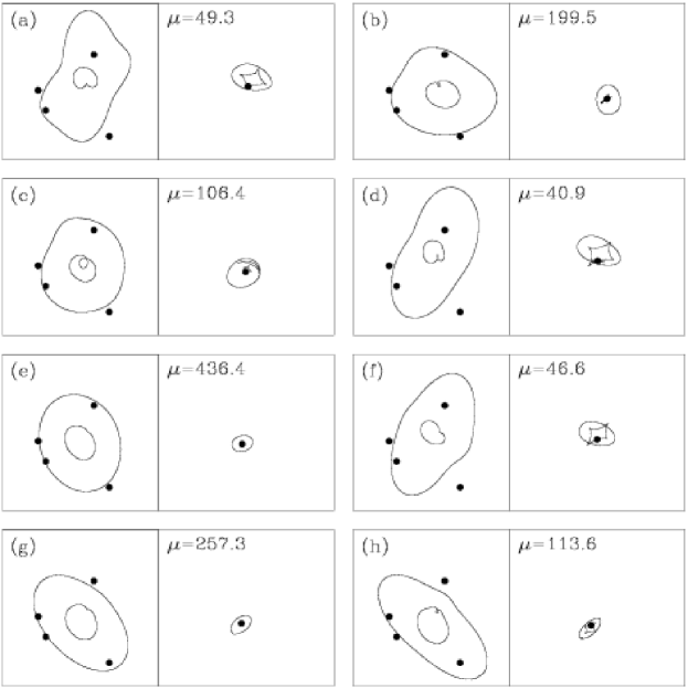
Figure 4: Critical curves and caustics for sample galaxy+cluster lens models with a cluster scale radius $r_{\rm s}=40\arcsec$. In each panel, the left-hand side shows the critical curves in the image plane, and the right-hand side shows the caustics in the source plane on the same scale. The points in the image plane show the observed image positions, and the point in the source plane shows the inferred source position. The value of $\mu$ gives the total magnification in each model.

Figure 4 shows critical curves and caustics for sample lens models. The critical curves are not well determined. The outer, tangential critical curve can point either northeast (panel e) or northwest (panel d), or it can have a complex shape (panel a). Sometimes there is just one inner, radial critical curve (panel e), but often there are two (panel c). The distance of the source from the caustic (and of the images from the critical curve) varies from model to model, so the total magnification can range from $\sim$50 to several hundred or even more. Finally, perhaps the most interesting qualitative result is that even the image parities are not uniquely determined. In most models (e.g., panels a–f) images A and D lie inside the critical curve and have negative parity while B and C lie outside the critical curve and have positive parity. However, in some models (e.g., panels g–h) the situation is reversed. Having ambiguous image parities is very rare in lens modeling.

Figure 5: Relation between the cluster scale radius $r_{\rm s}$ and lensing strength $\kappa_{\rm s}$. The solid line shows the predicted relation for clusters with the canonical median concentration, and the dotted lines show the 1$\sigma$ range due to the scatter in concentration. The labeled points show the value of $\log(M)$ (in units of $h^{-1}M_{\odot}$) at various points along the curve. The points show fitted values of $\kappa_{\rm s}$ for lens models with $r_{\rm s}=(10,20,30,40,50,60)$ arcsec. As in Figure 3, small points show all models, while boxes mark models where the model galaxy is roughly aligned with the observed galaxy.

So far we have only discussed models where the cluster has a scale radius $r_{\rm s}=40^{\prime\prime}$. We have also computed models with $r_{\rm s}=(10,20,30,50,60)$ arcsec and we find that all of the results are quite similar. To understand what value of the scale radius is reasonable, we must consider which (if any) of the models have physically plausible cluster parameters. Even though NFW models are formally specified by two parameters $r_{\rm s}$ and $\kappa_{\rm s}$, $N$-body simulations reveal that the two parameters are actually correlated. NFW models therefore appear to form a one-parameter family of models, although with some scatter which reflects the scatter of the concentration parameter $c_{\rm vir}=r_{\rm vir}/r_{\rm s}$ ($r_{\rm vir}$ is a virial radius of the cluster). Figure 5 shows the predicted relation between $r_{\rm s}$ and $\kappa_{\rm s}$, including the scatter. For comparison, it also shows the fitted values of $\kappa_{\rm s}$ in lens models with different scale radii. Models with $r_{\rm s}=10^{\prime\prime}$ or $20^{\prime\prime}$ require $\kappa_{\rm s}$ much larger than expected, corresponding to a halo that is too concentrated. Models with $r_{\rm s}\geq 30^{\prime\prime}$, by contrast, overlap with the predictions and thus are physically plausible. We can therefore conclude very roughly that the cluster component must have $r_{\rm s}\gtrsim 30^{\prime\prime}$ and a total virial mass $M\gtrsim 10^{14}\,h^{-1}\,M_{\odot}$.

Finally, we can use the models to predict the time delays between the images. The models always predict that the time delay between images C and D is the longest and the delay between A and B is the shortest. However, there is no robust prediction of the temporal ordering: most models predict that the sequence should be C–B–A–D, but a few models predict the reverse ordering D–A–B–C. This is a direct result of the ambiguity in the image parities, because the leading image is always a positive-parity image (e.g., Schneider et al. 1992). We note, however, that all of the models where the model galaxy is roughly aligned with the observed galaxy have the C–B–A–D ordering.

Figure 6: Predictions for the longest ($\Delta t_{CD}$) and shortest ($\Delta t_{BA}$) time delays, where $\Delta t_{ij}>0$ means image $i$ leads image $j$, and vice versa. Results are shown for models where the cluster has scale length $r_{\rm s}=(30,40,50,60)$ arcsec. As in Figure 3, small points show all models, while boxes mark models where the model galaxy is roughly aligned with the observed galaxy.

Figure 6 shows the predictions for the long and short time delays. The long delay between C and D can be anything up to $\sim\!3000\,h^{-1}$ days, while the short delay between A and B can be up to $\sim\!37\,h^{-1}$ days. For the models where the galaxy is roughly aligned with the observed galaxy, the two delays are approximately proportional to each other with $\Delta t_{CD}/\Delta t_{BA}=143\pm 16$. These results have several important implications. First, the A–B time delay should be on the order of weeks or months, so it should be very feasible to measure it, provided that the source has detectable variations. Measuring the A–B delay would be very useful because it would determine the temporal ordering, and thereby robustly determine the image parities. In addition, it would allow a good estimate of the long C–D delay and indicate whether attempting to measure that delay would be worthwhile. Second, the enormous range of predicted time delays means that constraining the Hubble constant with this system (Refsdal 1964a, b) will be difficult because of large systematic uncertainties in the lens models. Although Koopmans et al. (2003) recently showed that it is possible to obtain useful constraints on the Hubble constant even in a complex system with two mass components, the analysis is very complex and requires extensive data including not just the image positions and all of the time delays, but also an Einstein ring image and the velocity dispersion of one of the mass components. Even if we obtain such data for SDSS J1004+4112 in the near future, it seems likely that it will be difficult to obtain reliable constraints on the Hubble constant given the complexity of the lens potential in SDSS J1004+4112. The time delays, however, would still be extremely useful, because they would determine the temporal ordering and hence the image parities, and they would provide constraints that can rule out many of the models that are currently acceptable.

Appendix 14.C Summary

We have shown that reasonable mass models can successfully reproduce the observed properties of the lens. When we consider models that include both the cluster potential and the brightest cluster galaxy, we find a broad range of acceptable models. Despite the diversity in the models, we find several general and interesting conclusions. First, there appears to be a small ($\gtrsim\!4\,h^{-1}$ kpc) offset between the brightest cluster galaxy and the center of the cluster potential. Such an offset is fairly common in clusters (e.g., Postman & Lauer 1995). Second, the cluster potential is inferred to be elongated roughly North–South, which is consistent with the observed distribution of apparent member galaxies. Third, we found that a significant external shear $\gamma\sim 0.2$ is needed to fit the data, even when we allow the cluster potential to be elliptical. This may imply that the structure of the cluster potential outside of the images is more complicated than simple elliptical symmetry. Fourth, given the broad range of acceptable models, we cannot determine even the parities and temporal ordering of the images, much less the amplitudes of the time delays between the images. Measurements of any of the time delays would therefore provide powerful new constraints on the models. We note that the complexity of the lens potential means that the time delays will be more useful for constraining the mass model than for trying to measure the Hubble constant.

Our modeling results suggest that further progress will require new data (rather than refinements of current data). The interesting possibilities include catalogs of confirmed cluster members, X-ray observations, and weak lensing maps, not to mention measurement of time delays and confirmation of lensed arcs (either the possible arclets we have identified, or others). For instance, with an estimated cluster mass of $M\sim 3\times 10^{14}\,h^{-1}\,M_{\odot}$, the estimated X-ray bolometric flux is $S_{X}\sim 10^{-13}\,{\rm erg\,s^{-1}cm^{-2}}$, which means that the cluster should be accessible with the Chandra and XMM-Newton X-ray observatories; the excellent spatial of Chandra may be particularly useful for separating the diffuse cluster component from the bright quasar images (which have a total X-ray flux $S_{X}\sim 2\times 10^{-12}{\rm erg\,s^{-1}cm^{-2}}$ in the ROSAT All Sky Survey). The confirmation of lensed arclets would be very valuable, as they would provide many more pixels’ worth of constraints on the complicated lens potential. In principle, mapping radio jets in the quasar images could unambiguously reveal the image parities (e.g., Gorenstein et al. 1988; Garrett et al. 1994), but unfortunately the quasar appears to be radio quiet as it is not detected in radio sky surveys such as the FIRST survey (Becker, White, & Helfand 1995).

References

- Aaronson et al. (1986) Aaronson, M., Bothun, G., Mould, J., Huchra, J., Schommer, R. A., & Cornell, M. E. 1986, ApJ, 302, 536
- Abazajian et al. (2003) Abazajian, K., et al. 2003, AJ, 126, 2081
- Abazajian et al. (2004) Abazajian, K., et al. 2004, AJ, 128, 502
- Afshordi et al. (2004) Afshordi, N., Loh, Y., & Strauss, M. A. 2004, Phys. Rev. D, 69, 083524
- Allen & Fabian (1998) Allen, S. W. & Fabian, A. C. 1998, MNRAS, 297, L57
- Allen et al. (2002) Allen, S. W., Schmidt, R. W., & Fabian, A. C. 2002, MNRAS, 334, L11
- Allen et al. (2003) Allen, S. W., Schmidt, R. W., Fabian, A. C., & Ebeling, H. 2003, MNRAS, 342, 287
- Bacon et al. (2000) Bacon, D. J., Refregier, A. R., & Ellis, R. S. 2000, MNRAS, 318, 625
- Bacon et al. (2003) Bacon, D. J., Massey, R. J., Refregier, A. R., & Ellis, R. S. 2003, MNRAS, 344, 673
- Bahcall et al. (1992) Bahcall, J. N., Maoz, D., Doxsey, R., Schneider, D. P., Bahcall, N. A., Lahav, O., & Yanny, B. 1992, ApJ, 387, 56
- Bahcall et al. (2003a) Bahcall, N. A., et al. 2003a, ApJ, 585, 182
- Bahcall & Bode (2003b) Bahcall, N. A., & Bode, P. 2003b, ApJ, 588, L1
- Bardeen et al. (1986) Bardeen, J. M., Bond, J. R., Kaiser, N., & Szalay, A. S. 1986, ApJ, 304, 15
- Barkana et al. (1999) Barkana, R., Lehár, J., Falco, E. E., Grogin, N. A., Keeton, C. R., & Shapiro, I. I. 1999, ApJ, 520, 479
- Barkhouse & Hall (2001) Barkhouse, W. A., & Hall, P. B. 2001, AJ, 121, 2843
- Bartelmann & Weiss (1994) Bartelmann, M., & Weiss, A. 1994, A&A, 287, 1
- Bartelmann, Steinmetz, & Weiss (1995a) Bartelmann, M., Steinmetz, M., & Weiss, A. 1995a, A&A, 297, 1
- Bartelmann (1995b) Bartelmann, M. 1995b, A&A, 299, 11
- Bartelmann (1996) Bartelmann, M. 1996, A&A, 313, 697
- Bartelmann et al. (1998) Bartelmann, M., Huss, A., Colberg, J. M., Jenkins, A., & Pearce, F. R. 1998, A&A, 330, 1
- Bartelmann et al. (2003) Bartelmann, M., Meneghetti, M., Perrotta, F., Baccigalupi, C., & Moscardini, L. 2003, A&A, 409, 449
- Bartelmann & Meneghetti (2004) Bartelmann, M., & Meneghetti, M. 2004, A&A, 418, 413
- Becker et al. (1995) Becker, R. H., White, R. L., & Helfand, D. J. 1995, ApJ, 450, 559
- Bennett et al. (2003) Bennett, C. L., et al. 2003, ApJS, 148, 1
- Bernardi et al. (2003) Bernardi, M., et al. 2003, AJ, 125, 1817
- Bertin & Arnouts (1996) Bertin, E., & Arnouts, S. 1996, A&AS, 117, 393
- Binney (1985) Binney, J. 1985, MNRAS, 212, 767
- Blake & Glazebrook (2003) Blake, C., & Glazebrook, K. 2003, ApJ, 594, 665
- Blanton et al. (2003) Blanton, M. R., Lin, H., Lupton, R. H., Maley, F. M., Young, N., Zehavi, I., & Loveday, J. 2003, AJ, 125, 2276
- Blumenthal et al. (1986) Blumenthal, G. R., Faber, S. M., Flores, R., & Primack, J. R. 1986, ApJ, 301, 27
- Bode et al. (2001) Bode, P., Ostriker, J. P., & Turok, N. 2001, ApJ, 556, 93
- Boehm et al. (2004) Boehm, C., Hooper, D., Silk, J., Casse, M., & Paul, J. 2004, Phys. Rev. Lett., 92, 101301
- Bond et al. (1991) Bond, J. R., Cole, S., Efstathiou, G., & Kaiser, N. 1991, ApJ, 379, 440
- Borgani et al. (2001) Borgani, S., et al. 2001, ApJ, 561, 13
- Borgeest (1983) Borgeest, U. 1983, A&A, 128, 162
- Boughn & Crittenden (2004) Boughn, S., & Crittenden, R. 2004, Nature, 427, 45
- Bower (1991) Bower, R. G. 1991, MNRAS, 248, 332
- Bower et al. (1992) Bower, R. G., Lucey, J. R., & Ellis, R. S. 1992, MNRAS, 254, 601
- Boyle et al. (1988) Boyle, B. J., Shanks, T., & Peterson, B. A. 1988, MNRAS, 235, 935
- Boyle et al. (2000) Boyle, B. J., Shanks, T., Croom, S. M., Smith, R. J., Miller, L., Loaring, N., & Heymans, C. 2000, MNRAS, 317, 1014
- Bradač et al. (2002) Bradač, M., Schneider, P., Steinmetz, M., Lombardi, M., King, L. J., & Porcas, R. 2002, A&A, 388, 373
- Broadhurst et al. (2000) Broadhurst, T., Huang, X., Frye, B., & Ellis, R. 2000, ApJ, 534, L15
- Brown et al. (2003) Brown, M. L., Taylor, A. N., Bacon, D. J., Gray, M. E., Dye, S., Meisenheimer, K., & Wolf, C. 2003, MNRAS, 341, 100
- Browne et al. (2003) Browne, I. W. A., et al. 2003, MNRAS, 341, 13
- Bullock et al. (2001) Bullock, J. S., Kolatt, T. S., Sigad, Y., Somerville, R. S., Kravtsov, A. V., Klypin, A. A., Primack, J. R., & Dekel, A. 2001, MNRAS, 321, 559
- Buote et al. (2002) Buote, D. A., Jeltema, T. E., Canizares, C. R., & Garmire, G. P. 2002, ApJ, 577, 183
- Buote & Lewis (2004) Buote, D. A., & Lewis, A. D. 2004, ApJ, 604, 116
- Burke (1981) Burke, W. L. 1981, ApJ, 244, L1
- Burud et al. (1998) Burud, I., et al. 1998, ApJ, 501, L5
- Caldwell et al. (1998) Caldwell, R. R., Dave, R., & Steinhardt, P. J. 1998, Phys. Rev. Lett., 80, 1582
- Cao et al. (1999) Cao, L., Wei, J.-Y., & Hu, J.-Y. 1999, A&AS, 135, 243
- Carroll et al. (1992) Carroll, S. M., Press, W. H., & Turner, E. L. 1992, ARA&A, 30, 499
- Cen et al. (1994) Cen, R., Gott, J. R., Ostriker, J. P., & Turner, E. L. 1994, ApJ, 423, 1
- Cen (2001) Cen, R. 2001, ApJ, 546, L77
- Chae et al. (2002) Chae, K.-H., et al. 2002, Phys. Rev. Lett., 89, 151301
- Chae (2003) Chae, K.-H. 2003, MNRAS, 346, 746
- Chen (2003) Chen, D. 2003, ApJ, 587, L55
- Chen (2004) Chen, D. 2004, A&A, 418, 387
- Chen et al. (2003) Chen, J., Kravtsov, A. V., & Keeton, C. R. 2003, ApJ, 592, 24
- Chiba & Yoshii (1999) Chiba, M., & Yoshii, Y. 1999, ApJ, 510, 42
- Chiba (2002) Chiba, M. 2002, ApJ, 565, 17
- Chung et al. (1998) Chung, D. J. H., Kolb, E. W., & Riotto, A. 1998, Phys. Rev. Lett., 81, 4048
- Clowe & Schneider (2001) Clowe, D., & Schneider, P. 2001, A&A, 379, 384
- Clowe & Schneider (2002) Clowe, D., & Schneider, P. 2002, A&A, 395, 385
- Coc et al. (2002) Coc, A., Vangioni-Flam, E., Cassé, M., & Rabiet, M. 2002, Phys. Rev. D, 65, 043510
- Coc et al. (2004) Coc, A., Vangioni-Flam, E., Descouvemont, P., Adahchour, A., & Angulo, C. 2004, ApJ, 600, 544
- Cohn & Kochanek (2004) Cohn, J. D., & Kochanek, C. S. 2004, ApJ, 608, 25
- Colín et al. (2000) Colín, P., Avila-Reese, V., & Valenzuela, O. 2000, ApJ, 542, 622
- Colley et al. (1996) Colley, W. N., Tyson, J. A., & Turner, E. L. 1996, ApJ, 461, L83
- Cooke & Kantowski (1975) Cooke, J. H., & Kantowski, R. 1975, ApJ, 195, L11
- Cooray (1999) Cooray, A. R. 1999, ApJ, 524, 504
- Cooray et al. (2000) Cooray, A., Hu, W., & Miralda-Escudé, J. 2000, ApJ, 535, L9
- Cooray et al. (2004) Cooray, A., Huterer, D., & Baumann, D. 2004, Phys. Rev. D, 69, 027301
- Croft et al. (2002) Croft, R. A. C., Weinberg, D. H., Bolte, M., Burles, S., Hernquist, L., Katz, N., Kirkman, D., & Tytler, D. 2002, ApJ, 581, 20
- Czoske et al. (2002) Czoske, O., Moore, B., Kneib, J.-P., & Soucail, G. 2002, A&A, 386, 31
- Dahle et al. (2003) Dahle, H., Hannestad, S., & Sommer-Larsen, J. 2003, ApJ, 588, L73
- Dalal & Kochanek (2002) Dalal, N., & Kochanek, C. S. 2002, ApJ, 572, 25
- Dalal et al. (2004a) Dalal, N., Holder, G., & Hennawi, J. F. 2004a, ApJ, 609, 50
- Dalal & Keeton (2004b) Dalal, N., & Keeton, C. R. 2004b, ApJ, submitted (astro-ph/0312072)
- de Bernardis et al. (2000) de Bernardis, P., et al. 2000, Nature, 404, 955
- de Blok et al. (2001) de Blok, W. J. G., McGaugh, S. S., Bosma, A., & Rubin, V. C. 2001, ApJ, 552, L23
- de Blok & Bosma (2002) de Blok, W. J. G., & Bosma, A. 2002, A&A, 385, 816
- de Blok et al. (2003) de Blok, W. J. G., Bosma, A., & McGaugh, S. 2003, MNRAS, 340, 657
- de Blok (2004) de Blok, W. J. G., in the proceedings of “Dark Matter in Galaxies”, eds. S. Ryder et al., in press
- De Lucia et al. (2004) De Lucia, G., Kauffmann, G., Springel, V., White, S. D. M., Lanzoni, B., Stoehr, F., Tormen, G., & Yoshida, N. 2004, MNRAS, 348, 333
- de Vries et al. (2003) de Vries, W. H., Becker, R. H., & White, R. L. 2003, AJ, 126, 1217
- Doran (2003) Doran, M. 2003, preprint (astro-ph/0302138)
- Dressler (1980) Dressler, A. 1980, ApJ, 236, 351
- Dressler & Gunn (1992) Dressler, A., & Gunn, J. E. 1992, ApJS, 78, 1
- Efstathiou et al. (1988) Efstathiou, G., Frenk, C. S., White, S. D. M., & Davis, M. 1988, MNRAS, 235, 715
- Efstathiou & Bond (1999) Efstathiou, G., & Bond, J. R. 1999, MNRAS, 304, 75
- Einstein (1936) Einstein, A. 1936, \sci, 84, 506
- Eisenstein & Hu (1998) Eisenstein, D. J., & Hu, W. 1998, ApJ, 496, 605
- Eisenstein et al. (2001) Eisenstein, D. J., et al. 2001, AJ, 122, 2267
- Evans & Hunter (2002) Evans, N. W., & Hunter, C. 2002, ApJ, 575, 68
- Evans & Witt (2003) Evans, N. W., & Witt, H. J. 2003, MNRAS, 345, 1351
- Evrard et al. (2002) Evrard, A. E., et al. 2002, ApJ, 573, 7
- Falco et al. (1999) Falco, E. E., et al. 1999, ApJ, 523, 617
- Finoguenov et al. (2001) Finoguenov, A., Reiprich, T. H., & Böhringer, H. 2001, A&A, 368, 749
- Flores & Primack (1996) Flores, R. A., & Primack, J. R. 1996, ApJ, 457, L5
- Flores et al. (2000) Flores, R. A., Maller, A. H., & Primack, J. R. 2000, ApJ, 535, 555
- Font et al. (2001) Font, A. S., Navarro, J. F., Stadel, J., & Quinn, T. 2001, ApJ, 563, L1
- Fort et al. (1992) Fort, B., Le Févre, O., Hammer, F., & Cailloux, M. 1992, ApJ, 399, L125
- Fosalba et al. (2003) Fosalba, P., Gaztañaga, E., & Castander, F. J. 2003, ApJ, 597, L89
- Franx et al. (1997) Franx, M., Illingworth, G. D., Kelson, D. D., van Dokkum, P. G., & Tran, K. 1997, ApJ, 486, L75
- Freedman et al. (2001) Freedman, W. L., et al. 2001, ApJ, 553, 47
- Fukugita et al. (1990a) Fukugita, M., Futamase, T., & Kasai, M. 1990a, MNRAS, 246, 24P
- Fukugita et al. (1990b) Fukugita, M., Yamashita, K., Takahara, F., & Yoshii, Y. 1990b, ApJ, 361, L1
- Fukugita et al. (1995) Fukugita, M., Shimasaku, K., & Ichikawa, T. 1995, PASP, 107, 945
- Fukugita et al. (1996) Fukugita, M., Ichikawa, T., Gunn, J. E., Doi, M., Shimasaku, K., & Schneider, D. P. 1996, AJ, 111, 1748
- Fukushige & Makino (1997) Fukushige, T., & Makino, J. 1997, ApJ, 477, L9
- Fukushige & Makino (2001) Fukushige, T., & Makino, J. 2001, ApJ, 557, 533
- Fukushige & Makino (2003) Fukushige, T., & Makino, J. 2003, ApJ, 588, 674
- Fukushige et al. (2004) Fukushige, T., Kawai, A., & Makino, J. 2004, ApJ, 606, 625
- Futamase (1995) Futamase, T. 1995, \ptp, 93, 647
- Garrett et al. (1994) Garrett, M. A., Calder, R. J., Porcas, R. W., King, L. J., Walsh, D., & Wilkinson, P. N. 1994, MNRAS, 270, 457
- Gavazzi et al. (2003) Gavazzi, R., Fort, B., Mellier, Y., Pello, R., & Dantel-Fort, M. 2003, A&A, 403, 11
- Ghigna et al. (2000) Ghigna, S., Moore, B., Governato, F., Lake, G., Quinn, T., & Stadel, J. 2000, ApJ, 544, 616
- Gioia et al. (1998) Gioia, I. M., Shaya, E. J., Le Févre, O., Falco, E. E., Luppino, G. A., & Hammer, F. 1998, ApJ, 497, 573
- Gladders & Yee (2000) Gladders, M. D., & Yee, H. K. C. 2000, AJ, 120, 2148
- Gladders et al. (2003) Gladders, M. D., Hoekstra, H., Yee, H. K. C., Hall, P. B., & Barrientos, L. F. 2003, ApJ, 593, 48
- Gnedin & Hamilton (2002) Gnedin, N. Y., & Hamilton, A. J. S. 2002, MNRAS, 334, 107
- Golse et al. (2002) Golse, G., Kneib, J.-P., & Soucail, G. 2002, A&A, 387, 788
- Gondolo & Silk (1999) Gondolo, P., & Silk, J. 1999, Phys. Rev. Lett., 83, 1719
- Goodman (2000) Goodman, J. 2000, New Astronomy, 5, 103
- Gorenstein et al. (1988) Gorenstein, M. V., Cohen, N. L., Shapiro, I. I., Rogers, A. E. E., Bonometti, R. J., Falco, E. E., Bartel, N., & Marcaide, J. 1988, ApJ, 334, 42
- Goto et al. (2002) Goto, T. et al. 2002, AJ, 123, 1807
- Green et al. (2002) Green, P. J., et al. 2002, ApJ, 571, 721
- Gunn et al. (1998) Gunn, J. E., et al. 1998, AJ, 116, 3040
- Halverson et al. (2002) Halverson, N. W., et al. 2002, ApJ, 568, 38
- Hamana & Futamase (1997) Hamana, T., & Futamase, T. 1997, MNRAS, 286, L7
- Hamana et al. (2003) Hamana, T., et al. 2003, ApJ, 597, 98
- Hammer et al. (1997) Hammer, F., Gioia, I. M., Shaya, E. J., Teyssandier, P., Le Févre, O., & Luppino, G. A. 1997, ApJ, 491, 477
- Hanany et al. (2000) Hanany, S., et al. 2000, ApJ, 545, L5
- Harrison (1970) Harrison, E. R. 1970, Phys. Rev. D, 1, 2726
- Hattori et al. (1997a) Hattori, M., et al. 1997a, Nature, 388, 146
- Hattori et al. (1997b) Hattori, M., Watanabe, K., & Yamashita, K. 1997b, A&A, 319, 764
- Hayashi et al. (2003) Hayashi, E., Navarro, J. F., Taylor, J. E., Stadel, J., & Quinn, T. 2003, ApJ, 584, 541
- Hayashi et al. (2004) Hayashi, E., et al. 2004, MNRAS, submitted (astro-ph/0310576)
- Hernquist & Katz (1989) Hernquist, L., & Katz, N. 1989, ApJS, 70, 419
- Hewett et al. (1998) Hewett, P. C., Foltz, C. B., Harding, M. E., & Lewis, G. F. 1998, AJ, 115, 383
- Heymans et al. (2004) Heymans, C., Brown, M., Heavens, A., Meisenheimer, K., Taylor, A., & Wolf, C. 2004, MNRAS, 347, 895
- Hinshaw & Krauss (1987) Hinshaw, G., & Krauss, L. M. 1987, ApJ, 320, 468
- Hoekstra et al. (2002) Hoekstra, H., Yee, H. K. C., & Gladders, M. D. 2002, ApJ, 577, 595
- Hoekstra et al. (2004) Hoekstra, H., Yee, H. K. C., & Gladders, M. D. 2004, ApJ, 606, 67
- Hogg et al. (2001) Hogg, D. W., Finkbeiner, D. P., Schlegel, D. J., & Gunn, J. E. 2001, AJ, 122, 2129
- Hu et al. (2000) Hu, W., Barkana, R., & Gruzinov, A. 2000, Phys. Rev. Lett., 85, 1158
- Huterer & Ma (2004a) Huterer, D., & Ma, C. 2004a, ApJ, 600, L7
- Huterer & Keeton (2004b) Huterer, D., & Keeton, C. R. 2004b, in preparation
- Ichikawa et al. (2004) Ichikawa, K., Kawasaki, M., & Takahashi, F. 2004, Phys. Rev. D, submitted (astro-ph/0402522)
- Ichiki et al. (2003) Ichiki, K., Garnavich, P. M., Kajino, T., Mathews, G. J., & Yahiro, M. 2003, Phys. Rev. D, 68, 083518
- Ichiki et al. (2004) Ichiki, K., Oguri, M., & Takahashi, K. 2004, Phys. Rev. Lett., in press (astro-ph/040316)
- Ikebe et al. (2002) Ikebe, Y., Reiprich, T. H., Böhringer, H., Tanaka, Y., & Kitayama, T. 2002, A&A, 383, 773
- Inada et al. (2003a) Inada, N., et al. 2003a, AJ, 126, 666
- Inada et al. (2003b) Inada, N., et al. 2003b, Nature, 426, 810
- Inada et al. (2004a) Inada, N., et al. 2004a, AJ, submitted
- Inada (2004b) Inada, N., 2004b, PhD thesis, University of Tokyo
- Inoue & Chiba (2003) Inoue, K. T., & Chiba, M. 2003, ApJ, 591, L83
- Jain & Taylor (2003) Jain, B., & Taylor, A. 2003, Phys. Rev. Lett., 91, 141302
- Jarvis et al. (2003) Jarvis, M., Bernstein, G. M., Fischer, P., Smith, D., Jain, B., Tyson, J. A., & Wittman, D. 2003, AJ, 125, 1014
- Jeltema et al. (2001) Jeltema, T. E., Canizares, C. R., Bautz, M. W., Malm, M. R., Donahue, M., & Garmire, G. P. 2001, ApJ, 562, 124
- Jenkins et al. (2001) Jenkins, A., Frenk, C. S., White, S. D. M., Colberg, J. M., Cole, S., Evrard, A. E., Couchman, H. M. P., & Yoshida, N. 2001, MNRAS, 321, 372
- Jing & Suto (2000a) Jing, Y. P., & Suto, Y. 2000a, ApJ, 529, L69
- Jing (2000b) Jing, Y. P. 2000b, ApJ, 535, 30
- Jing & Suto (2002) Jing, Y. P., & Suto, Y. 2002, ApJ, 574, 538
- Johnston et al. (2003) Johnston, D. E., et al. 2003, AJ, 126, 2281
- Kamionkowski et al. (1995) Kamionkowski, M., Griest, K., Jungman, G., & Sadoulet, B. 1995, Phys. Rev. Lett., 74, 5174
- Kamionkowski & Liddle (2000) Kamionkowski, M., & Liddle, A. R. 2000, Phys. Rev. Lett., 84, 4525
- Kaplinghat et al. (2000) Kaplinghat, M., Knox, L., & Turner, M. S. 2000, Phys. Rev. Lett., 85, 3335
- Kashikawa et al. (2002) Kashikawa, N., et al. 2002, PASJ, 54, 819
- Kashikawa et al. (2003) Kashikawa, N., et al. 2003, AJ, 125, 53
- Kassiola & Kovner (1993) Kassiola, A., & Kovner, I. 1993, ApJ, 417, 450
- Kawano et al. (2004) Kawano, Y., Oguri, M., Matsubara, T., & Ikeuchi, S. 2004, PASJ, 56, 253
- Kayser & Refsdal (1983) Kayser, R., & Refsdal, S. 1983, A&A, 128, 156
- Kazantzidis et al. (2004) Kazantzidis, S., Kravtsov, A. V., Zentner, A. R., Allgood, B., Nagai, D., & Moore, B. 2004, ApJ, 611, L73
- Keeton et al. (1997) Keeton, C. R., Kochanek, C. S., & Seljak, U. 1997, ApJ, 482, 604
- Keeton (1998a) Keeton, C. R. 1998a, Ph. D. thesis, Harvard University
- Keeton et al. (1998b) Keeton, C. R., Kochanek, C. S., & Falco, E. E. 1998b, ApJ, 509, 561
- Keeton & Madau (2001a) Keeton, C. R., & Madau, P. 2001a, ApJ, 549, L25
- Keeton (2001b) Keeton, C. R. 2001b, ApJ, 561, 46
- Keeton (2001c) Keeton, C. R. 2001c, ApJ, 562, 160
- Keeton (2001d) Keeton, C. R. 2001d, preprint (astro-ph/0102340)
- Keeton (2002) Keeton, C. R. 2002, ApJ, 575, L1
- Keeton (2003a) Keeton, C. R. 2003a, ApJ, 582, 17
- Keeton & Winn (2003b) Keeton, C. R., & Winn, J. N. 2003b, ApJ, 590, 39
- Keeton et al. (2003c) Keeton, C. R., Gaudi, B. S., & Petters, A. O. 2003c, ApJ, 598, 138
- Kelson et al. (2002) Kelson, D. D., Zabludoff, A. I., Williams, K. A., Trager, S. C., Mulchaey, J. S., & Bolte, M. 2002, ApJ, 576, 720
- King & Ellis (1985) King, C. R., & Ellis, R. S. 1985, ApJ, 288, 456
- Kirkman et al. (2003) Kirkman, D., Tytler, D., Suzuki, N., O’Meara, J. M., & Lubin, D. 2003, ApJS, 149, 1
- Kitayama & Suto (1996) Kitayama, T., & Suto. Y. 1996, ApJ, 469, 480
- Klypin et al. (1999) Klypin, A., Kravtsov, A. V., Valenzuela, O., & Prada, F. 1999, ApJ, 522, 82
- Klypin et al. (2001) Klypin, A., Kravtsov, A. V., Bullock, J. S., & Primack, J. R. 2001, ApJ, 554, 903
- Knop et al. (2003) Knop, R. A., et al. 2003, ApJ, 598, 102
- Kochanek et al. (1995a) Kochanek, C. S., Falco, E. E., & Schild, R. 1995a, ApJ, 452, 109
- Kochanek (1995b) Kochanek, C. S. 1995b, ApJ, 453, 545
- Kochanek (1996) Kochanek, C. S. 1996, ApJ, 466, 638
- Kochanek et al. (1999) Kochanek, C. S., Falco, E. E., & Muñoz, J. A. 1999, ApJ, 510, 590
- Kochanek & White (2001) Kochanek, C. S., & White, M. 2001, ApJ, 559, 531
- Kochanek (2002a) Kochanek, C. S. 2002a, preprint (astro-ph/0204043)
- Kochanek (2002b) Kochanek, C. S. 2002b, in Proc. Workshop, The Shapes of Galaxies and their Halos, ed. P. Natarjan (Singapore: World Scientific), p. 62
- Kochanek & Dalal (2004a) Kochanek, C. S., & Dalal, N. 2004a, ApJ, 610, 69
- Kochanek et al. (2004b) Kochanek, C. S., Falco, E. E., Impey, C., Lehar, J., McLeod, B., & Rix, H.-W. 2004b, CASTLES Survery, http://cfa-www.harvard.edu/castles/
- Komatsu & Seljak (2002) Komatsu, E., & Seljak, U. 2002, MNRAS, 336, 1256
- Komatsu et al. (2003) Komatsu, E., et al. 2003, ApJS, 148, 119
- Koopmans et al. (2003) Koopmans, L. V. E., Treu, T., Fassnacht, C. D., Blandford, R. D., & Surpi, G. 2003, ApJ, 599, 70
- Kormann et al. (1994) Kormann, R., Schneider, P., & Bartelmann, M. 1994, A&A, 284, 285
- Kravtsov, Gnedin, & Klypin (2004) Kravtsov, A. V., Gnedin, O. Y., & Klypin, A. A. 2004, ApJ, 609, 482
- Kuhlen et al. (2004) Kuhlen, M., Keeton, C. R., & Madau, P. 2004, ApJ, 601, 104
- Kuo et al. (2004) Kuo, C. L., et al. 2004, ApJ, 600, 32
- Kusenko & Shaposhnikov (1998) Kusenko, A., & Shaposhnikov, M. 1998, \plb, 418, 46
- Lacey & Ostriker (1985) Lacey, C. G., & Ostriker, J. P. 1985, ApJ, 299, 633
- Lacey & Cole (1993) Lacey, C., & Cole, S. 1993, MNRAS, 262, 627
- Lacey & Cole (1994) Lacey, C., & Cole, S. 1994, MNRAS, 271, 676
- Lambas et al. (1992) Lambas, D. G., Maddox, S. J., & Loveday, J. 1992, MNRAS, 258, 404
- Le Févre et al. (1994) Le Févre, O., Hammer, F., Angonin, M. C., Gioia, I. M., & Luppino, G. A. 1994, ApJ, 422, L5
- Lewis et al. (2002) Lewis, G. F., Carilli, C., Papadopoulos, P., & Ivison, R. J. 2002, MNRAS, 330, L15
- Lewis et al. (2003) Lewis, A. D., Buote, D. A., & Stocke, J. T. 2003, ApJ, 586, 135
- Li & Ostriker (2002) Li, L. X., & Ostriker, J. P. 2002, ApJ, 566, 652
- Li & Ostriker (2003) Li, L. X., & Ostriker, J. P. 2003, ApJ, 595, 603
- Lilly et al. (1995) Lilly, S. J., Tresse, L., Hammer, F., Crampton, D., & Le Févre, O. 1995, ApJ, 455, 108
- Łokas et al. (2004) Łokas, E. L., Bode, P., & Hoffman, Y. 2004, MNRAS, 349, 595
- Lopes & Miller (2004) Lopes, A. M., & Miller, L. 2004, MNRAS, 348, 519
- Luppino & Gioia (1992) Luppino, G. A. & Gioia, I. M. 1992, A&A, 265, L9
- Luppino et al. (1993) Luppino, G. A., Gioia, I. M., Annis, J., Le Févre, O., & Hammer, F. 1993, ApJ, 416, 444
- Luppino et al. (1999) Luppino, G. A., Gioia, I. M., Hammer, F., Le Févre, O., & Annis, J. A. 1999, A&AS, 136, 117
- Lupton et al. (1999) Lupton, R. H., Gunn, J. E., & Szalay, A. S. 1999, AJ, 118, 1406
- Lupton et al. (2001) Lupton, R., Gunn, J. E., Ivezić, Z., Knapp, G. R., Kent, S., & Yasuda, N. 2001, in ASP Conf. Ser. 238, Astronomical Data Analysis Software and Systems X, ed. F. R. Harnden, Jr., F. A. Primini, and H. E. Payne (San Francisco: Astr. Soc. Pac.), p. 269
- Lynds & Petrosian (1986) Lynds, R., & Petrosian, V. 1986, BAAS, 18, 1014
- Ma (2003) Ma, C.-P. 2003, ApJ, 584, L1
- Macciò (2004) Macciò, A. V. 2004, MNRAS, submitted (astro-ph/0402657)
- Madau et al. (1999) Madau, P., Haardt, F., & Rees, M. J. 1999, ApJ, 514, 648
- Mao & Schneider (1998) Mao, S., & Schneider, P. 1998, MNRAS, 295, 587
- Mao et al. (2004) Mao, S., Jing, Y.-P., Ostriker, J. P., & Weller, J. 2004, ApJ, 604, L5
- Maoz et al. (1997) Maoz, D., Rix, H.-W., Gal-Yam, A., & Gould, A. 1997, ApJ, 486, 75
- Marlow et al. (2000) Marlow, D. R., Rusin, D., Jackson, N., Wilkinson, P. N., & Browne, I. W. A. 2000, AJ, 119, 2629
- Massey et al. (2004) Massey, R., Refregier, A., Bacon, D., & Ellis, R. 2004, MNRAS, submitted (astro-ph/0404195)
- Mathez et al. (1992) Mathez, G., Fort, B., Mellier, Y., Picat, J.-P., & Soucail, G. 1992, A&A, 256, 343
- Mathis et al. (2004) Mathis, H., Diego, J. M., & Silk, J. 2004, MNRAS, submitted (astro-ph/0402461)
- Matsubara & Szalay (2003) Matsubara, T., & Szalay, A. S. 2003, Phys. Rev. Lett., 90, 021302
- Matting (1958) Matting, W. 1958, Astron. Nachr., 284, 109
- Meneghetti et al. (2000) Meneghetti, M., Bolzonella, M., Bartelmann, M., Moscardini, L., & Tormen, G. 2000, MNRAS, 314, 338
- Meneghetti et al. (2001) Meneghetti, M., Yoshida, N., Bartelmann, M., Moscardini, L., Springel, V., Tormen, G., & White S. D. M. 2001, MNRAS, 325, 435
- Meneghetti et al. (2003a) Meneghetti, M., Bartelmann, M., & Moscardini, L. 2003a, MNRAS, 340, 105
- Meneghetti et al. (2003b) Meneghetti, M., Bartelmann, M., & Moscardini, L. 2003b, MNRAS, 346, 67
- Metcalf & Zhao (2002) Metcalf, R. B., & Zhao, H. 2002, ApJ, 567, L5
- Metcalf et al, (2004) Metcalf, R. B., Moustakas, L. A., Bunker, A. J., & Parry, I. R. 2004, ApJ, 607, 43
- Miller et al. (2004) Miller, L., Lopes, A. M., Smith, R. J., Croom, S. M., Boyle, B. J., Shanks, T., & Outram, P. 2004, MNRAS, 348, 395
- Miralda-Escudé (1993a) Miralda-Escudé, J. 1993a, ApJ, 403, 497
- Miralda-Escudé (1993b) Miralda-Escudé, J. 1993b, ApJ, 403, 509
- Miralda-Escudé (1995) Miralda-Escudé, J. 1995, ApJ, 438, 514
- Miralda-Escudé (2002) Miralda-Escudé, J. 2002, ApJ, 564, 60
- Mitchell et al. (2004) Mitchell, J. L., Keeton, C. R., Frieman, J. A, & Sheth, R. K. 2004, ApJ, submitted (astro-ph/0401138)
- Miyazaki et al. (2002a) Miyazaki, S., et al. 2002a, ApJ, 580, L97
- Miyazaki et al. (2002b) Miyazaki, S., et al. 2002b, PASJ, 54, 833
- Molikawa et al. (1999) Molikawa, K., Hattori, M., Kneib, J. P., & Yamashita, K. 1999, A&A, 351, 413
- Molikawa & Hattori (2001) Molikawa, K., & Hattori, M. 2001, ApJ, 559, 544
- Moore et al. (1999a) Moore, B., Ghigna, S., Governato, F., Lake, G., Quinn, T., Stadel, J., & Tozzi, P. 1999a, ApJ, 524, L19
- Moore et al. (1999b) Moore, B., Quinn, T., Governato, F., Stadel, J., & Lake, G. 1999b, MNRAS, 310, 1147
- Morgan et al. (2003) Morgan, N. D., Snyder, J. A., & Reens, L. H. 2003, AJ, 126, 2145
- Mortlock et al. (1999) Mortlock, D. J., Webster, R. L., & Francis, P. J. 1999, MNRAS, 309, 836
- Mortlock & Webster (2000) Mortlock, D. J., & Webster, R. L. 2000, MNRAS, 319, 872
- Muñoz et al. (2001) Muñoz, J. A., et al. 2001, ApJ, 546, 769
- Mushotzky & Scharf (1997) Mushotzky, R. F. & Scharf, C. A. 1997, ApJ, 482, L13
- Myers et al. (1995) Myers, S. T., et al. 1995, ApJ, 447, L5
- Myers et al. (2003) Myers, S. T., et al. 2003, MNRAS, 341, 1
- Nakamura & Suto (1997) Nakamura, T. T., & Suto, Y. 1997, \ptp, 97, 49
- Narayan & White (1988) Narayan, R., & White, S. D. M. 1988, MNRAS, 231, 97P
- Navarro et al. (1995) Navarro, J. F., Frenk, C. S., & White, S. D. M. 1995, MNRAS, 275, 720
- Navarro et al. (1996) Navarro, J. F., Frenk, C. S., & White, S. D. M. 1996, ApJ, 462, 563
- Navarro et al. (1997) Navarro, J. F., Frenk, C. S., & White, S. D. M. 1997, ApJ, 490, 493
- Navarro et al. (2004) Navarro, J. F., et al. 2004, MNRAS, 349, ,1039
- Nolta et al. (2004) Nolta, M. R., et al. 2004, ApJ, 608, 10
- Novicki et al. (2002) Novicki, M. C., Sornig, M., & Henry, J. P. 2002, AJ, 124, 2413
- Ofek et al. (2001) Ofek, E. O., Maoz, D., Prada, F., Kolatt, T., & Rix, H.-W. 2001, MNRAS, 324, 463
- Ofek et al. (2002) Ofek, E. O., Rix, H.-W., Maoz, D., & Prada, F. 2002, MNRAS, 337, 1163
- Oguri et al. (2001) Oguri, M., Taruya, A., & Suto, Y. 2001, ApJ, 559, 572
- Oguri et al. (2002a) Oguri, M., Taruya, A., Suto, Y., & Turner, E. L. 2002a, ApJ, 568, 488
- Oguri (2002b) Oguri, M. 2002b, ApJ, 573, 51
- Oguri (2002c) Oguri, M. 2002c, ApJ, 580, 2
- Oguri et al. (2003a) Oguri, M., Suto, Y., & Turner, E. L. 2003a, ApJ, 583, 584
- Oguri & Kawano (2003b) Oguri, M., & Kawano, Y. 2003b, MNRAS, 338, L25
- Oguri (2003c) Oguri, M. 2003c, MNRAS, 339, L23
- Oguri et al. (2003d) Oguri, M., Takahashi, K., Ohno, H., & Kotake, K. 2003d, ApJ, 597, 645
- Oguri et al. (2003e) Oguri, M., Lee, J., & Suto, Y. 2003e, ApJ, 599, 7
- Oguri et al. (2004a) Oguri, M., et al. 2004a, ApJ, 605, 78
- Oguri et al. (2004b) Oguri, M., et al. 2004b, PASJ, 56, 399
- Oguri & Keeton (2004c) Oguri, M., & Keeton, C. R. 2004c, ApJ, 610, 663
- Oguri & Lee (2004d) Oguri, M., & Lee, J. 2004d, MNRAS, in press (astro-ph/0401628)
- Okamoto & Habe (1999) Okamoto, T., & Habe, A. 1999, ApJ, 516, 591
- Oke et al. (1995) Oke, J. B., et al. 1995, PASP, 107, 375
- Ostriker & Peebles (1973) Ostriker, J. P., & Peebles, P. J. E. 1973, ApJ, 186, 467
- Ostriker & Steinhardt (2003) Ostriker, J. P., & Steinhardt, P. 2003, \sci, 300, 1909
- Ota et al. (2004) Ota, N., Pointecouteau, E., Hattori, M., & Mitsuda, K. 2004, ApJ, 601, 120
- Park (2004) Park, C.-G. 2004, MNRAS, 349, 313
- Patnaik et al. (1992) Patnaik, A. R., Browne, I. W. A., Wilkinson, P. N., & Wrobel, J. M. 1992, MNRAS, 254, 655
- Peacock & Heavens (1990) Peacock, J. A., & Heavens, A. F. 1990, MNRAS, 243, 133
- Peacock (1999) Peacock, J. A. 1999, Cosmological Physics (Cambridge: Cambridge University Press)
- Pearson et al. (2003) Pearson, T. J., et al. 2003, ApJ, 591, 556
- Peccei & Quinn (1977) Peccei, R. D., & Quinn, H. R. 1977, Phys. Rev. Lett., 38, 1440
- Peebles (1980) Peebles, P. J. E. 1980, The Large-Scale Structure of the Universe (Princeton: Princeton Universe Press)
- Peebles (2000) Peebles, P. J. E. 2000, ApJ, 534, L127
- Peiris et al. (2003) Peiris, H. V., et al. 2003, ApJS, 148, 213
- Percival et al. (2001) Percival, W. J., et al. 2001, MNRAS, 327, 1297
- Perlmutter et al. (1999) Perlmutter, S., et al. 1999, ApJ, 517, 565
- Peterson & Wandel (1999) Peterson, B. M., & Wandel, A. 1999, ApJ, 521, L95
- Phillips (1993) Phillips, M. M. 1993, ApJ, 413, L105
- Phillips et al. (2001a) Phillips, P. M., Browne, I. W. A., & Wilkinson, P. N. 2001a, MNRAS, 321, 187
- Phillips et al. (2001b) Phillips, P. M., et al. 2001b, MNRAS, 328, 1001
- Pier et al. (2003) Pier, J. R., Munn, J. A., Hindsley, R. B., Hennessy, G. S., Kent, S. M., Lupton, R. H., & Ivezić, Ž. 2003, AJ, 125, 1559
- Pierpaoli et al. (2003) Pierpaoli, E., Borgani, S., Scott, D., & White, M. 2003, MNRAS, 342, 163
- Pindor et al. (2003) Pindor, B., Turner, E. L., Lupton, R. H., & Brinkmann, J. 2003, AJ, 125, 2325
- Pindor et al. (2004) Pindor, B., et al. 2004, AJ, 127, 1318
- Poli et al. (2001) Poli, F., Menci, N., Giallongo, E., Fontana, A., Cristiani, S., & D’Odorico, S. 2001, ApJ, 551, L45
- Pope et al. (2004) Pope, A. C., et al. 2004, ApJ, 607, 655
- Porciani & Madau (2000) Porciani, C., & Madau, P. 2000, ApJ, 532, 679
- Postman & Lauer (1995) Postman, M., & Lauer, T. R. 1995, ApJ, 440, 28
- Power et al. (2003) Power, C., Navarro, J. F., Jenkins, A., Frenk, C. S., White, S. D. M., Springel, V., Stadel, J., & Quinn, T. 2003, MNRAS, 338, 14
- Press & Schechter (1974) Press, W. H., & Schechter, P. 1974, ApJ, 187, 425
- Press et al. (1992) Press, W. H., Teukolsky, S. A., Vetterling, W. T., & Flannery, B. P. 1992, Numerical Recipes in Fortran (Cambridge: Cambridge Univ. Press)
- Ratra & Peebles (1988) Ratra, B., & Peebles, P. J. E. 1988, Phys. Rev. D, 37, 3406
- Rees & Ostriker (1977) Rees, M. J., & Ostriker, J. P. 1977, MNRAS, 179, 541
- Reese et al. (2002) Reese, E. D., Carlstrom, J. E., Joy, M., Mohr, J. J., Grego, L., & Holzapfel, W. L. 2002, ApJ, 581, 53
- Refregier et al. (2002) Refregier, A., Rhodes, J., & Groth, E. J. 2002, ApJ, 572, L131
- Refsdal (1964a) Refsdal, S. 1964a, MNRAS, 128, 307
- Refsdal (1964b) Refsdal, S. 1964b, MNRAS, 128, 307
- Refsdal (1966) Refsdal, S. 1966, MNRAS, 132, 101
- Rhodes et al. (2004) Rhodes, J., Refregier, A., Collins, N. R., Gardner, J. P., Groth, E. J., & Hill, R. S. 2004, ApJ, 605, 29
- Richards et al. (2002) Richards, G. T., et al. 2002, AJ, 123, 2945
- Richards et al. (2004a) Richards, G. T., et al. 2004a, AJ, 127, 1305
- Richards et al. (2004b) Richards, G. T., et al. 2004b, ApJ, 610, 679
- Riess et al. (1998) Riess, A. G., et al. 1998, AJ, 116, 1009
- Riess et al. (2001) Riess, A. G., et al. 2001, ApJ, 560, 49
- Riess et al. (2004) Riess, A. G., et al. 2004, ApJ, 607, 665
- Riotto & Tkachev (2000) Riotto, A., & Tkachev, I. 2000, \plb, 484, 177
- Rusin & Ma (2001a) Rusin, D. & Ma, C. 2001a, ApJ, 549, L33
- Rusin & Tegmark (2001b) Rusin, D., & Tegmark, M. 2001b, ApJ, 553, 709
- Rusin (2002) Rusin, D. 2002, ApJ, 572, 705
- Rubin & Ford (1970) Rubin, V. C., & Ford, W. K. J. 1970, ApJ, 159, 379
- Rubin et al. (1985) Rubin, V. C., Burstein, D., Ford, W. K., & Thonnard, N. 1985, ApJ, 289, 81
- Ryan et al. (2000) Ryan, S. G., Beers, T. C., Olive, K. A., Fields, B. D., & Norris, J. E. 2000, ApJ, 530, L57
- Sand et al. (2002) Sand, D. J., Treu, T., & Ellis, R. S. 2002, ApJ, 574, L129
- Sand et al. (2004) Sand, D. J., Treu, T., Simth, G. P., & Ellis, R. S. 2004, ApJ, 604, 88
- Sarbu et al. (2001) Sarbu, N., Rusin, D., & Ma, C.-P. 2001, ApJ, 561, L147
- Sasaki (1993) Sasaki, M. 1993, \ptp, 90, 753
- Sasaki & Takahara (1993) Sasaki, S., & Takahara, F. 1993, MNRAS, 262, 681
- Sasaki (1996) Sasaki, S. 1996, PASJ, 48, L119
- Sawicki et al. (1997) Sawicki, M. J., Lin, H., & Yee, H. K. C. 1997, AJ, 113, 1
- Schechter (1976) Schechter, P. 1976, ApJ, 203, 297
- Schechter & Wambsganss (2002) Schechter, P. L., & Wambsganss, J. 2002, ApJ, 580, 685
- Schmidt et al. (1995) Schmidt, M., Schneider, D. P., & Gunn, J. E. 1995, AJ, 110, 68
- Schneider (1984) Schneider, P. 1984, A&A, 140, 119
- Schneider (1985) Schneider, P. 1985, A&A, 143, 413
- Schneider et al. (1992) Schneider, P., Ehlers, J., & Falco, E. E. 1992, Gravitational Lenses (New York: Springer)
- Schramm (1990) Schramm, T. 1990, A&A, 231, 19
- Schuecker et al. (2003) Schuecker, P., Böhringer, H., Collins, C. A., & Guzzo, L. 2003, A&A, 398, 867
- Scoccimarro et al. (2004) Scoccimarro, R., Sefusatti, E., & Zaldarriaga, M. 2004, Phys. Rev. D, 69, 103513
- Scott et al. (2000) Scott, J., Bechtold, J., Dobrzycki, A., & Kulkarni, V. P. 2000, ApJS, 130, 67
- Scranton et al. (2004) Scranton, R., et al. 2004, Phys. Rev. Lett., submitted (astro-ph/0307335)
- Seitz et al. (1994) Seitz, S., Schneider, P., & Ehlers, J. 1994, Class. Quant. Grav., 11, 2345
- Seljak (2002) Seljak, U. 2002, MNRAS, 337, 769
- Sereno (2002) Sereno, M. 2002, A&A, 393, 757
- Shapiro & Iliev (2000) Shapiro, P. R., & Iliev, I. T. 2000, ApJ, 542, L1
- Sheth & Tormen (1999) Sheth, R. K., & Tormen, G. 1999, MNRAS, 308, 119
- Sheth et al. (2003) Sheth, R. K., et al. 2003, ApJ, 594, 225
- Shimizu et al. (2003) Shimizu, M., Kitayama, T., Sasaki, S., & Suto, Y. 2003, ApJ, 590, 197
- Simon et al. (2003) Simon, J. D., Bolatto, A. D., Leroy, A., & Blitz, L. 2003, ApJ, 596, 957
- Smith et al. (2001) Smith, G. P., Kneib, J., Ebeling, H., Czoske, O., & Smail, I. 2001, ApJ, 552, 493
- Smith et al. (2002) Smith, J. A., et al. 2002, AJ, 123, 2121
- Somerville (2002) Somerville, R. S. 2002, ApJ, 572, L23
- Soucail et al. (1987) Soucail, G., Fort, B., Mellier, Y., & Picat, J. P. 1987, A&A, 172, L14
- Spergel & Steinhardt (2000) Spergel, D. N., & Steinhardt P. J. 2000, Phys. Rev. Lett., 84, 3760
- Spergel et al. (2003) Spergel, D. N., et al. 2003, ApJS, 148, 175
- Springel et al. (2001) Springel, V., White, S. D. M., Tormen, G., & Kauffmann, G. 2001, MNRAS, 328, 726
- Squires et al. (1996) Squires, G., Kaiser, N., Babul, A., Fahlman, G., Woods, D., Neumann, D. M., & Boehringer, H. 1996, ApJ, 461, 572
- Stoehr et al. (2002) Stoehr, F., White, S. D. M., Tormen, G., & Springel, V. 2002, MNRAS, 335, L84
- Stoughton et al. (2002) Stoughton, C., et al. 2002, AJ, 123, 485
- Strauss et al. (2002) Strauss, M. A., et al. 2002, AJ, 124, 1810
- Sugiyama (1995) Sugiyama, N. 1995, ApJS, 100, 281
- Surpi et al. (1996) Surpi, G. C., Harari, D. D., & Frieman, J. A. 1996, ApJ, 464, 54
- Sutherland & Dopita (1993) Sutherland, R. S., & Dopita, M. A. 1993, ApJS, 88, 253
- Suto (2001) Suto, Y. 2001, in the proceedings of “AMiBA 2001: High-z Clusters, Missing Baryons, and CMB Polarization”, eds. L.-W. Chen, C.-P. Ma, K.-W. Ng & U.-L. Pen (San Francisco: ASP), 195
- Suto (2003) Suto, Y. 2003, in the proceedings of “Matter and Energy in Clusters of Galaxies”, eds. S. Bowyer & C.-Y. Hwang (San Francisco: ASP), 370
- Swaters et al. (2003) Swaters, R. A., Madore, B. F., van den Bosch, F. C., & Balcells, M. 2003, ApJ, 583, 732
- Takada & Jain (2003) Takada, M., & Jain, B. 2003, MNRAS, 344, 857
- Takahashi & Chiba (2001) Takahashi, R., & Chiba, T. 2001, ApJ, 563, 489
- Takahashi et al. (2004a) Takahashi, K., Oguri, M., & Ichiki, K. 2004a, MNRAS, 352, 311
- Takahashi et al. (2004b) Takahashi, K., Oguri, M., Kotake, K., & Ohno, H. 2004b, J. Cosmology Astropart. Phys, submitted (astro-ph/0305260)
- Tamura et al. (2000) Tamura, T., Makishima, K., Fukazawa, Y., Ikebe, Y., & Xu, H. 2000, ApJ, 535, 602
- Tegmark et al. (2004) Tegmark, M, et al. 2004, ApJ, 606, 702
- Tonry (1991) Tonry, J. L. 1991, ApJ, 373, L1
- Tormen et al. (1998) Tormen, G., Diaferio, A., & Syer, D. 1998, MNRAS, 299, 728
- Torri et al. (2004) Torri, E., Meneghetti, M., Bartelmann, M., Moscardini, L., Rasia, E., & Tormen, G. 2004, MNRAS, 349, 476
- Turner (1980) Turner, E. L. 1980, ApJ, 242, L135
- Turner et al. (1984) Turner, E. L., Ostriker, J. P., & Gott, J. R. 1984, ApJ, 284, 1
- Turner (1990) Turner, E. L. 1990, ApJ, 365, L43
- Tyson (1988) Tyson, J. A. 1988, AJ, 96, 1 1
- Tyson et al. (1990) Tyson, J. A., Wenk, R. A., & Valdes, F. 1990, ApJ, 349, L1
- Tyson et al. (1998) Tyson, J. A., Kochanski, G. P., & Dell’Antonio I. P. 1998, ApJ, 498, L107
- Vanden Berg (1983) Vanden Berg, D. A. 1983, ApJS, 51, 29
- Vanden Berk et al. (2001) Vanden Berk, D. E., et al. 2001, AJ, 122, 549
- Vanden Berk et al. (2004) Vanden Berk, D. E., et al. 2004, ApJ, 601, 692
- van den Bosch & Swaters (2001) van den Bosch, F. C., & Swaters, R. A. 2001, MNRAS, 325, 1017
- van Waerbeke et al. (2000) van Waerbeke, L. et al. 2000, A&A, 358, 30
- Vielva et al. (2004) Vielva, P., Martinez-Gonzalez, E., Barreiro, R. B., Sanz, J. L., & Cayon, L. 2004, ApJ, 609, 22
- Walsh et al. (1979) Walsh, D., Carswell, R. F., & Weymann, R. J. 1979, Nature, 279, 381
- Wambsganss et al. (1995) Wambsganss, J., Cen, R., Ostriker, J. P., & Turner, E. L. 1995, Science, 268, 274
- Wambsganss et al. (2004) Wambsganss, J., Bode, P., & Ostriker, J. P. 2004, ApJ, 606, L93
- Wechsler et al. (2002) Wechsler, R. H., Bullock, J. S., Primack, J. R., Kravtsov, A. V., & Dekel, A. 2002, ApJ, 568, 52
- Weinberg & Katz (2002) Weinberg, M. D., & Katz, N. 2002, ApJ, 580, 627
- White (2002) White, M. 2002, ApJS, 143, 241
- White et al. (1993) White, S. D. M., Navarro, J. F., Evrard, A. E., & Frenk, C. S. 1993, Nature, 366, 429
- Williams et al. (1999) Williams, L. L. R., Navarro, J. F., & Bartelmann, M. 1999, ApJ, 527, 535
- Winn et al. (2004) Winn, J. N., Rusin, D., & Kochanek, C. S. 2004, Nature, 427, 613
- Wittman et al. (2000) Wittman, D. M., Tyson, J. A., Kirkman, D., Dell’Antonio, I., & Bernstein, G. 2000, Nature, 405, 143
- Wittman et al. (2001) Wittman, D., Tyson, J. A., Margoniner, V. E., Cohen, J. G., & Dell’Antonio, I. P. 2001, ApJ, 557, L89
- Wu & Hammer (1993) Wu, X.-P., & Hammer, F. 1993, MNRAS, 262, 187
- Wu & Mao (1996) Wu, X.-P., & Mao, S. 1996, ApJ, 463, 404
- Wyithe et al. (2001) Wyithe, J. S. B., Turner, E. L., & Spergel, D. N. 2001, ApJ, 555, 504
- Wyithe & Loeb (2002a) Wyithe, J. S. B., & Loeb, A. 2002a, Nature, 417, 923
- Wyithe & Loeb (2002b) Wyithe, J. S. B., & Loeb, A. 2002b, ApJ, 577, 57
- Yokoyama (2000) Yokoyama, J. 2000, Phys. Rev. D, 62, 123509
- Yonehara et al. (2003) Yonehara, A., Umemura, M., & Susa, H. 2003, PASJ, 55, 1059
- Yoo et al. (2004) Yoo, J., Chanamé, J., & Gould, A. 2004, ApJ, 601, 311
- York et al. (2000) York, D. G., et al. 2000, AJ, 120, 1579
- Yoshida et al. (2000a) Yoshida, N., Springel, V., White, S. D. M., & Tormen, G. 2000a, ApJ, 535, L103
- Yoshida et al. (2000b) Yoshida, N., Springel, V., White, S. D. M., & Tormen, G. 2000b, ApJ, 544, L87
- Yoshida et al. (2003) Yoshida, N., Sokasian, A., Hernquist, L., & Springel, V. 2003, ApJ, 598, 73
- Zaritsky & Gonzalez (2003) Zaritsky, D. & Gonzalez, A. H. 2003, ApJ, 584, 691
- Zel’dovich (1972) Zel’dovich, Y. B. 1972, MNRAS, 160, 1P
- Zhao (1996) Zhao, H. S. 1996, MNRAS, 278, 488
- Zentner & Bullock (2003) Zentner, A. R., & Bullock, J. S. 2003, ApJ, 598, 49
- Zhdanov & Surdej (2001) Zhdanov, V. I., & Surdej, J. 2001, A&A, 372, 1
- Zwicky (1933) Zwicky, F. 1933, Helv. Phys. Acta, 6, 110
- Zwicky (1937a) Zwicky, F. 1937a, Phys. Rev., 51, 290
- Zwicky (1937b) Zwicky, F. 1937b, Phys. Rev., 51, 679