The Luminosity and Color Dependence of the Galaxy Correlation Function

Abstract

We study the luminosity and color dependence of the galaxy two-point correlation function in the Sloan Digital Sky Survey (SDSS), starting from a sample of $\sim 200,000$ galaxies over 2500 deg². We concentrate our analysis on volume-limited subsamples of specified luminosity ranges, for which we measure the projected correlation function ${w_{p}(r_{p})}$, which is directly related to the real space correlation function $\xi(r)$. The amplitude of ${w_{p}(r_{p})}$ rises continuously with luminosity from $M_{r}\approx-17.5$ to $M_{r}\approx-22.5$, with the most rapid increase occurring above the characteristic luminosity $L_{*}$ ($M_{r}\approx-20.5$). Over the scales $0.1\,h^{-1}\;{\rm Mpc}<r_{p}<10\,h^{-1}\;{\rm Mpc}$, the measurements for samples with $M_{r}>-22$ can be approximated, imperfectly, by power-law three-dimensional correlation functions $\xi(r)=(r/r_{0})^{-\gamma}$ with $\gamma\approx 1.8$ and $r_{0}(L_{*})\approx 5.0\,h^{-1}\;{\rm Mpc}$. The brightest subsample, $-23<M_{r}<-22$, has a significantly steeper $\xi(r)$. When we divide samples by color, redder galaxies exhibit a higher amplitude and steeper correlation function at all luminosities. The correlation amplitude of blue galaxies increases continuously with luminosity, but the luminosity dependence for red galaxies is less regular, with bright red galaxies exhibiting the strongest clustering at large scales and faint red galaxies exhibiting the strongest clustering at small scales. We interpret these results using halo occupation distribution (HOD) models assuming concordance cosmological parameters. For most samples, an HOD model with two adjustable parameters fits the ${w_{p}(r_{p})}$ data better than a power-law, explaining inflections at $r_{p}\sim 1-3\,h^{-1}\;{\rm Mpc}$ as the transition between the one-halo and two-halo regimes of $\xi(r)$. The implied minimum mass for a halo hosting a central galaxy more luminous than $L$ grows steadily, with $M_{\rm min}\propto L$ at low luminosities and a steeper dependence above $L_{*}$. The mass at which a halo has, on average, one satellite galaxy brighter than $L$ is $M_{1}\approx 23M_{\rm min}(L)$, at all luminosities. These results imply a conditional luminosity function (at fixed halo mass) in which central galaxies lie far above a Schechter function extrapolation of the satellite population. The HOD model fits nicely explain the color dependence of ${w_{p}(r_{p})}$ and the cross correlation between red and blue galaxies. For galaxies with $M_{r}<-21$, halos slightly above $M_{\rm min}$ have blue central galaxies, while more massive halos have red central galaxies and predominantly red satellite populations. The fraction of blue central galaxies increases steadily with decreasing luminosity and host halo mass. The strong clustering of faint red galaxies follows from the fact that nearly all of them are satellite systems in high mass halos. The HOD fitting results are in good qualitative agreement with the predictions of numerical and semi-analytic models of galaxy formation.

1 Introduction

Over the course of many decades, studies of large scale structure have established a dependence of galaxy clustering on morphological type (e.g., Hubble 1936; Zwicky et al. 1968; Davis & Geller 1976; Dressler 1980; Postman & Geller 1984; Einasto 1991; Guzzo et al. 1997; Willmer, da Costa & Pellegrini 1998; Zehavi et al. 2002; Goto et al. 2003), luminosity (e.g., Davis et al. 1988; Hamilton 1988; White, Tully, & Davis 1988; Einasto 1991; Park et al. 1994; Loveday et al. 1995; Guzzo et al. 1997; Benoist et al. 1996; Norberg et al. 2001; Zehavi et al. 2002), color (e.g., Willmer, da Costa & Pellegrini 1998; Brown, Webster & Boyle 2000; Zehavi et al. 2002), and spectral type (e.g., Norberg et al. 2002; Budavari et al. 2003; Madgwick et al. 2003). Galaxies with bulge-dominated morphologies, red colors, and spectral types indicating old stellar populations preferentially reside in dense regions, and they exhibit stronger clustering even on the largest scales because these dense regions are themselves biased tracers of the underlying matter distribution (Kaiser, 1984). Luminous galaxies cluster more strongly than faint galaxies, with the difference becoming marked above the characteristic luminosity $L_{*}$ of the Schechter (1976) luminosity function, but the detailed luminosity dependence has been difficult to establish because of the limited dynamic range even of large galaxy redshift surveys. The dependence of clustering on galaxy properties is a fundamental constraint on theories of galaxy formation, providing clues to the role of initial conditions and environmental influences in determining these properties. A detailed understanding of this dependence is also crucial to any attempt to constrain cosmological models with galaxy redshift surveys, since different types of galaxies trace the underlying large scale structure of the dark matter distribution in different ways.

Achieving this understanding is one of the central design goals of the Sloan Digital Sky Survey (SDSS; York et al. 2000), which provides high quality photometric information and redshifts for hundreds of thousands of galaxies, sufficient to allow high precision clustering measurements for many distinct classes of galaxies. In this paper we analyze the luminosity and color dependence of galaxy clustering in a sample of $\sim 200,000$ galaxies drawn from the SDSS, roughly corresponding to the main galaxy sample (Strauss et al., 2002) of the Second Data Release (DR2; Abazajian et al. 2004). Our methods are similar to those used in our study of clustering in an early sample of $\sim 30,000$ SDSS galaxies (Zehavi et al. 2002, hereafter Z02) and in studies of the luminosity, spectral type, and color dependence of clustering in the Two-Degree Field Galaxy Redshift Survey (2dFGRS; Colless et al. 2001) by Norberg et al. (2001, 2002), Madgwick et al. (2003), and Hawkins et al. (2003). Specifically, we concentrate on the projected correlation function ${w_{p}(r_{p})}$, where integration of the redshift space correlation function ${\xi(r_{p},\pi)}$ over the redshift dimension $\pi$ yields a quantity that depends only on the real space correlation function $\xi(r)$ (Davis & Peebles, 1983).

Examining traditional large scale structure statistics for different classes of galaxies complements studies of the correlation between galaxy properties and the local environment (Dressler, 1980; Postman & Geller, 1984; Einasto, & Einasto, 1987; Whitmore, Gilmore, & Jones, 1993; Lewis et al., 2002). Studies using the SDSS have allowed precise quantification of many of the trends recognized in earlier galaxy surveys, and the size and detail of the SDSS data set have allowed some qualitatively new results to emerge. Hogg et al. (2003) show that the local density increases sharply with luminosity at the bright end of the luminosity function and depends mainly on color for lower luminosity systems, with faint red galaxies in particular occupying high density regions. Blanton et al. (2005a) demonstrate that the dependence of local density on galaxy morphology and surface brightness can be largely understood as a consequence of the luminosity and color dependence, since these quantities themselves correlate strongly with luminosity and color. Goto et al. (2003) further examine the morphology-density relation in the SDSS and show that the transition from late to intermediate type populations occurs at moderate overdensity and the transition from intermediate to early types occurs at high overdensity. Studies using the SDSS spectroscopic properties reveal that star formation rates decrease sharply in high density environments (Gomez et al., 2003; Kauffmann et al., 2004) and that luminous AGN arise in systems with large bulges but relatively low density environments (Miller et al., 2003; Kauffmann et al., 2004). Our focus on the projected two-point correlation function at scales of $r\lesssim 30\,h^{-1}\;{\rm Mpc}$ also complements Tegmark et al.’s (2004a) examination of the luminosity dependence of the large scale galaxy power spectrum, and Kayo et al.’s (2004) study of the luminosity, color, and morphology dependence of the two-point and three-point correlation functions in redshift space.

Section 3 takes a traditional, empirical approach to our task. We measure ${w_{p}(r_{p})}$ for the full, flux-limited data sample and for volume-limited subsets with different luminosity and color cuts, and we fit the measurements with power-laws, which generally provide a good but not perfect description at $r_{p}\lesssim 20\,h^{-1}\;{\rm Mpc}$ (Zehavi et al. 2004, hereafter Z04; see also Hawkins et al. 2003; Gaztañaga & Juszkiewicz 2001). Figures 11 and 14 below summarize our empirical results on the luminosity and color dependence of the projected correlation function.

In section 4, we interpret these measurements in the framework of the Halo Occupation Distribution (HOD; see, e.g., Ma & Fry 2000; Peacock & Smith 2000; Seljak 2000; Scoccimarro et al. 2001; Berlind & Weinberg 2002). The HOD formalism describes the “bias” relation between galaxies and mass in terms of the probability distribution $P(N|M)$ that a halo of virial mass $M$ contains $N$ galaxies of a given type, together with prescriptions for the relative bias of galaxies and dark matter within virialized halos. (Throughout this paper, we use the term “halo” to refer to a structure of overdensity $\rho/\bar{\rho}\sim 200$ in approximate dynamical equilibrium, which may contain a single galaxy or many galaxies.) This description is complete, in the sense that any galaxy clustering statistic on any scale can be predicted given an HOD and a cosmological model, using numerical simulations or analytic methods. The HOD approach to modeling ${w_{p}(r_{p})}$ comes with strong theoretical priors: we assume a $\Lambda$CDM cosmological model (inflationary cold dark matter with a cosmological constant) with parameters motivated by independent measurements, and we adopt parameterized forms of the HOD loosely motivated by contemporary theories of galaxy formation (Kauffmann, Nusser, & Steinmetz, 1997; Kauffman et al., 1999; Benson et al., 2000; Berlind et al., 2003; Kravtsov et al., 2004; Zheng et al., 2004). HOD modeling transforms ${w_{p}(r_{p})}$ data on galaxy pair counts into a physical relation between galaxies and dark matter halos, and it sets the stage for detailed tests of galaxy formation models and sharpened cosmological parameter constraints that draw simultaneously on a range of galaxy clustering statistics. Jing, Mo, & Börner (1998) pioneered HOD modeling of correlation function data in their study of the Las Campanas Redshift Survey, using an $N$-body approach. HOD modeling (or the closely related “conditional luminosity function” method) has since been applied to interpret clustering data from a number of surveys at low and high redshift (e.g., Jing & Börner 1998; Jing, Börner, & Suto 2002; Bullock, Wechsler, & Somerville 2002; Moustakas & Somerville 2002; van den Bosch, Yang, & Mo 2003a; Magliocchetti & Porciani 2003; Yan, Madgwick, & White 2003; Zheng 2004; Porciani, Magliocchetti, & Norberg 2004). In Z04, we used this approach to show that the observed deviations of the correlation function of $M_{r}<-21$ SDSS galaxies from a power-law form have a natural explanation in terms of the transition between galaxy pairs within a single virialized halo and galaxy pairs in separate halos.

Section 2 describes our data samples and methods. Section 3 presents the empirical results for the galaxy correlation function. Section 4 describes the details and results of the HOD modeling. Section 5 presents a summary of our results, comparison to previous work, and directions for future investigation.

2 Observations and Analysis

2.1 Data

The Sloan Digital Sky Survey (SDSS; York et al. 2000) is an ongoing project that aims to map nearly a quarter of the sky in the northern Galactic cap, and a small portion of the southern Galactic cap, using a dedicated 2.5 meter telescope located at Apache Point Observatory in New Mexico. A drift-scanning mosaic CCD camera (Gunn et al., 1998) is used to image the sky in five photometric bandpasses (Fukugita et al., 1996; Smith et al., 2002) to a limiting magnitude of $r\sim 22.5$. The imaging data are processed through a series of pipelines that perform astrometric calibration (Pier et al., 2003), photometric reduction (Lupton et al., 2001), and photometric calibration (Hogg et al. 2001), and objects are then selected for spectroscopic followup using specific algorithms for the main galaxy sample (Strauss et al., 2002), luminous red galaxy sample (Eisenstein et al., 2001), and quasars (Richards et al., 2002). To a good approximation, the main galaxy sample consists of all galaxies with Petrosian magnitude $r<17.77$. The targets are assigned to spectroscopic plates (tiles) using an adaptive tiling algorithm (Blanton et al., 2003a) and observed with a pair of fiber-fed spectrographs. Spectroscopic data reduction and redshift determination are performed by automated pipelines. Redshifts are measured with a success rate greater than $99\%$ and with estimated accuracy of $30\,{\rm km}\;{\rm s}^{-1}$. A summary description of the hardware, pipelines, and data outputs can be found in Stoughton et al. (2002).

Considerable effort has been invested in preparing the SDSS redshift data for large-scale structure studies (see, e.g., Blanton et al. 2005b; Tegmark et al. 2004a, Appendix A). The radial selection function is derived from the sample selection criteria using the K-corrections of Blanton et al. (2003b) and a modified version of the evolving luminosity function model of Blanton et al. (2003c). All magnitudes are corrected for Galactic extinction (Schlegel et al., 1998). We K-correct and evolve the luminosities to rest-frame magnitudes at $z=0.1$, near the median redshift of the sample. When we create volume-limited samples below, we include a galaxy if its evolved, redshifted spectral energy distribution would put it within the main galaxy sample’s apparent magnitude and surface brightness limits at the limiting redshift of the sample. The angular completeness is characterized carefully for each sector (a unique region of overlapping spectroscopic plates) on the sky. An operational constraint of using the fibers to obtain spectra is that no two fibers on the same plate can be closer than $55^{\prime\prime}$. This fiber collision constraint is partly alleviated by having roughly a third of the sky covered by overlapping plates, but it still results in $\sim 7\%$ of targeted galaxies not having a measured redshift. These galaxies are assigned the redshift of their nearest neighbor. We show below that this treatment is adequate for our purposes.

The clustering measurements in this paper are based on SDSS Large Scale Structure sample12, based on data taken as of July 2002 (essentially equivalent to the Second Data Release, DR2, Abazajian et al. 2004). It includes 204,584 galaxies over 2497 deg² of the sky. The angular coverage of this sample can be seen in Figure 1. This can be compared to the much smaller sky coverage of the sample analyzed in Z02 (its figure 1, $\sim 28\%$ of current area). The details of the construction and illuminating plots of the LSS sample are described by Tegmark et al. (2004a; §2 and Appendix A). Throughout the paper, when measuring distances we refer to comoving separations, and for all distance calculations and absolute magnitude definitions we adopt a flat $\Lambda$CDM model with $\Omega_{m}=0.3$. We quote distances in $\,h^{-1}\;{\rm Mpc}$ (where $h\equiv H_{0}/100\,\,{\rm km}\;{\rm s}^{-1}\;{\rm Mpc}^{-1}$), and we use $h=1$ to compute absolute magnitudes; one should add $5\log h$ to obtain magnitudes for other values of $H_{0}$.

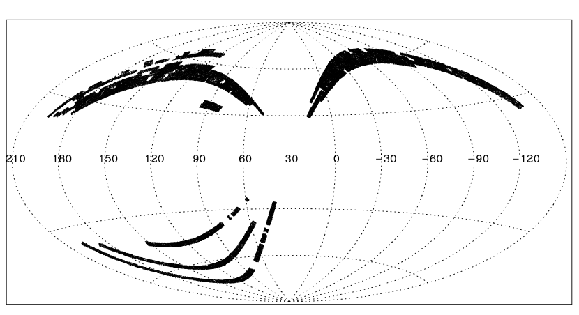
Figure 1: An Aitoff projection of our galaxy sample in Galactic coordinates.

We carry out some analyses of a full, flux-limited sample, with $14.5\leq r\lesssim 17.77$, with the bright limit imposed to avoid small incompleteness associated with galaxy deblending. The survey’s faint-end apparent magnitude limit varies slightly over the area of the sample, as the target selection criteria changed during the early phases of the survey. The radial completeness is computed independently for each of these regions and taken into account appropriately in our analysis. We have verified that our results do not change substantively if we cut the sample to a uniform flux limit of 17.5 (as done for simplicity in previous SDSS large-scale structure analyses), but we choose to incorporate the most expansive limits and gain in statistical accuracy. We also impose an absolute magnitude cut of $-22<M_{r}<-19$ (for $h=1$), thus limiting our analysis to a broad but well-defined range of absolute magnitudes around $M_{*}$ ($-20.44$; Blanton et al. 2003c), and reducing the effects of luminosity dependent bias within the sample. This cut maintains the majority of the galaxies in the sample, extending roughly from $(1/4)L_{*}$ to $4L_{*}$. We use galaxies in the redshift range $0.02<z<0.167$, resulting in a total of $154,014$ galaxies.

In addition to the flux-limited sample, we analyze a set of volume-limited subsamples that span a wider absolute magnitude range. For a given luminosity bin we discard the galaxies that are too faint to be included at the far redshift limit or too bright to be included at the near limit, so that the clustering measurement describes a well defined class of galaxies observed throughout the sample volume. We further cut these samples by color, using the K-corrected ${g-r}$ color as a separator into blue and red populations. In addition to luminosity-bin samples, we utilize a set of luminosity-threshold samples, which are volume-limited samples of all galaxies brighter than a given threshold. This set is particularly useful for the HOD modeling in § 4. For these samples we relax the bright flux limit to $r>10.5$; otherwise the sample volumes become too small as the lower redshift limit for the most luminous objects approaches the upper redshift limit of the faintest galaxies. While there are occasional problems with galaxy deblending or saturation at $r<14.5$, the affected galaxies are a small fraction of the total samples, and we expect the impact on clustering measurements to be negligible.

2.2 Clustering Measures

We calculate the galaxy correlation function on a two-dimensional grid of pair separations parallel ($\pi$) and perpendicular ($r_{p}$) to the line of sight. To estimate the background counts expected for unclustered objects while accounting for the complex survey geometry, we generate random catalogs with the detailed radial and angular selection functions of the samples. We estimate $\xi(r_{p},\pi)$ using the Landy & Szalay (1993) estimator

$$\xi(r_{p},\pi)=\frac{DD-2DR+RR}{RR},$$ (1)

where DD, DR and RR are the suitably normalized numbers of weighted data-data, data-random and random-random pairs in each separation bin. For the flux-limited sample we weight pairs using the minimum variance scheme of Hamilton (1993).

To learn about the real-space correlation function, we follow standard practice and compute the projected correlation function

$$w_{p}(r_{p})=2\int_{0}^{\infty}d\pi\,\xi(r_{p},\pi).$$ (2)

In practice we integrate up to $\pi=40\,h^{-1}\;{\rm Mpc}$, which is large enough to include most correlated pairs and gives a stable result by suppressing noise from distant, uncorrelated pairs. The projected correlation function can in turn be related to the real-space correlation function, ${\xi(r)}$,

$$w_{p}(r_{p})=2\int_{0}^{\infty}dy\,\xi\left[(r_{p}^{2}+y^{2})^{1/2}\right]=2\int_{r_{p}}^{\infty}r\,dr\,{\xi(r)}(r^{2}-{r_{p}}^{2})^{-1/2}$$ (3)

(Davis & Peebles, 1983). In particular, for a power-law $\xi(r)=(r/r_{0})^{-\gamma}$, one obtains

$$w_{p}(r_{p})=r_{p}\left(\frac{r_{p}}{r_{0}}\right)^{-\gamma}\Gamma\left(\frac{1}{2}\right)\Gamma\left(\frac{\gamma-1}{2}\right)\,\Bigr{/}\,\Gamma\left(\frac{\gamma}{2}\right),$$ (4)

allowing us to infer the best-fit power-law for ${\xi(r)}$ from $w_{p}$. The above measurement methods are those used in Z02, to which we refer the reader for more details.

Alternatively, one can directly invert $w_{p}$ to get ${\xi(r)}$ independent of the power-law assumption. Equation (3) can be recast as

$${\xi(r)}=-\frac{1}{\pi}\int_{r}^{\infty}{w_{p}}^{\prime}(r_{p})({r_{p}}^{2}-r^{2})^{-1/2}dr_{p}$$ (5)

(e.g., Davis & Peebles 1983). We calculate the integral analytically by linearly interpolating between the binned ${w_{p}(r_{p})}$ values, following Saunders, Rowan-Robinson & Lawrence (1992). As this is still a somewhat approximate treatment, we focus our quantitative modeling on ${w_{p}(r_{p})}$.

We estimate statistical errors on our different measurements using jackknife resampling. We define 104 spatially contiguous subsamples of the full data set, each covering approximately 24 deg² on the sky, and our jackknife samples are then created by omitting each of these subsamples in turn. The covariance error matrix is estimated from the total dispersion among the jackknife samples,

$${\rm Covar}(\xi_{i},\xi_{j})=\frac{N-1}{N}\sum_{l=1}^{N}({\xi_{i}}^{l}-{\bar{\xi}_{i}})({\xi_{j}}^{l}-{\bar{\xi}_{j}}),$$ (6)

where $N=104$ in our case, and $\bar{\xi}_{i}$ is the mean value of the statistic ${\xi}_{i}$ measured in the samples ($\xi$ denotes here the statistic at hand, whether it is $\xi$ or $w_{p}$). In Z02 we used $N=10$ for a much smaller sample, while here the larger number, 104, enables us to estimate the full covariance matrix and still allows each excluded subvolume to be sufficiently large.

Following Z02, we repeat and extend the tests with mock catalogs to check the reliability of the jackknife error estimates. We use 100 mock catalogs with the same geometry and angular completeness as the SDSS sample and similar clustering properties, created using the PTHalos method of Scoccimarro & Sheth (2002). (The mocks correspond to the sample analyzed in Z04, a slightly earlier version of our current sample, but we expect the results to be the same). For each mock catalog we calculate the projected correlation function ${w_{p}(r_{p})}$ and compute jackknife error estimates with the same procedure that we use for the SDSS data. Figure 2 compares these error estimates to the “true” errors, defined as the dispersion among the 100 ${w_{p}(r_{p})}$ estimates from the fully independent mock catalogs. The jackknife estimates recover the true errors reasonably well for most separations (with $\sim 20\%\ 1\sigma$ scatter for the diagonal elements), without gross systematics. The jackknife errors seem to fare well also for the off-diagonal elements of the covariance error matrix, but with larger deviations. Since fits can be sensitive to off-diagonal elements when errors are strongly correlated, we will present some fits below using both the full jackknife covariance matrix and the diagonal elements alone. For a specified clustering model, the mock catalog approach is probably the best way to assess agreement of the model with the data. However, the jackknife approach is much more practical when analyzing multiple samples that have different sizes and clustering properties, as it automatically accounts for these differences without requiring a new clustering model in each case. The tests presented here indicate that parameter errors derived using the jackknife error estimates should be representative of the true statistical errors. We have verified this expectation using the SDSS data sample of Z04, finding that the jackknife covariance matrix produces fits and $\chi^{2}$ values similar to those obtained with a mock catalog covariance matrix, for either power-law or HOD model fitting.

Figure 2: Accuracy of jackknife error estimates on ${w_{p}(r_{p})}$, tested using the PTHalos mock catalogs. Points and errorbars show the mean and 1$\sigma$ scatter of the error estimates derived by applying our jackknife procedure to 100 mock catalogs, divided by the “true” errors defined by the scatter in ${w_{p}(r_{p})}$ among the 100 fully independent catalogs. The upper left panel shows diagonal terms in the covariance matrix, and other panels show terms one, two, and four elements from the diagonal as indicated.

Another issue we re-visited with simulations is the effect of fiber collisions. As mentioned above, we are unable to obtain redshifts of approximately $7\%$ of the galaxies because of the finite fiber size constraints; when two galaxies lie within $55^{\prime\prime}$ of each other, one is selected at random for spectroscopic observations. At $cz=50,000\,{\rm km}\;{\rm s}^{-1}$, the outer edge of our flux-limited sample, $55^{\prime\prime}$ corresponds to a comoving transverse separation of $0.13\,h^{-1}\;{\rm Mpc}$, and we thus restrict our measurements to separations larger than that. We assign to each “collided” (unobserved) galaxy the redshift of its nearest neighboring galaxy in angle. This approach is roughly equivalent to double weighting the galaxies for which we do obtain redshifts, but using the angular position of the unobserved galaxy better preserves the small scale pair distribution (see further discussion in Z02 and Strauss et al. 2002). In Z02 we tested this procedure using the tile overlap regions, where redshifts of collided galaxies are obtained when the area of sky is reobserved, and found this to be an adequate treatment: residual systematics for the redshift space correlation function were considerably smaller than the statistical errors, and this was even more true for ${w_{p}(r_{p})}$. We have since carried out improved tests using mock catalogs created from the White (2002) $\Lambda$CDM N-body simulation, which was run using a TreePM code in a periodic box of $300\,h^{-1}\;{\rm Mpc}$ on a side. We impose on it the SDSS sample12 mask and populate galaxies in dark matter halos (as in Berlind & Weinberg 2002) using a realistic HOD model derived from the $M_{r}<-20$ volume-limited SDSS sample (see §4). We identify galaxies that would have been collided according to the $55^{\prime\prime}$ fiber separation criterion. Figure 3 shows the ${w_{p}(r_{p})}$ estimate for this mock catalog corrected using our standard treatment, divided by the “true” ${w_{p}(r_{p})}$ calculated from the mock catalog with no galaxies eliminated by fiber collisions. The correction procedure works spectacularly well, with any residual bias being much smaller than the statistical errors on scales above our adopted minimum separation. The correction is important, however, as simply discarding the collided galaxies causes ${w_{p}(r_{p})}$ to be underestimated at all scales, especially $r_{p}\lesssim 1\,h^{-1}\;{\rm Mpc}$. Our correction works particularly well for ${w_{p}(r_{p})}$ because it is integrated over the line-of sight direction. The post-correction biases can be larger for other statistics — e.g., the redshift-space correlation function shows a small systematic deviation at $s\lesssim 1\,h^{-1}\;{\rm Mpc}$, though this is still well within the statistical uncertainty.

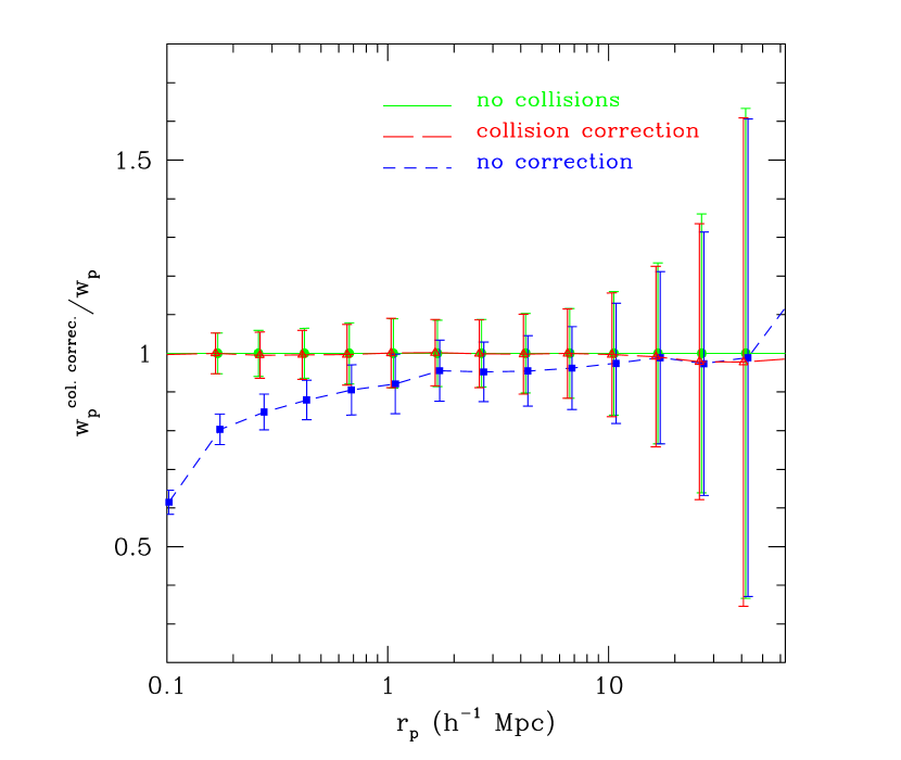
Figure 3: Test of the accuracy of our correction for fiber collisions, using a mock catalog drawn from a high resolution $N$-body simulation. The (green) solid line and errorbars denote the exemplary ideal case obtained for the full mock catalog, with no galaxies eliminated by fiber collisions. Errorbars throughout are obtained by jackknife resampling. The (red) long-dashed line and errorbars show the ${w_{p}(r_{p})}$ estimate from a mock catalog that includes fiber collisions, corrected using the same procedure we apply to the data, divided by ${w_{p}(r_{p})}$ for the full catalog. No systematic effect is present for scales above our minimum separation. The (blue) short-dashed line and square symbols with errorbars show the case where we apply no correction for collisions but simply drop the collided galaxies from the catalog.

3 The Galaxy Correlation Function

3.1 Clustering Results for the Flux-Limited Sample

Figure 4 shows contours of the correlation function as a function of projected $(r_{p})$ and line-of-sight ($\pi$) separation for our full flux-limited sample, where we bin $r_{p}$ and $\pi$ in linear bins of $2\,h^{-1}\;{\rm Mpc}$. One can clearly see the effects of redshift distortions in ${\xi(r_{p},\pi)}$. At small projected separations the contours are elongated along the line of sight due to small-scale virial motions in clusters, the so-called “finger-of-God” effect. At large projected separations ${\xi(r_{p},\pi)}$ shows compression in the $\pi$ direction caused by coherent large-scale streaming (Sargent & Turner, 1977; Kaiser, 1987; Hamilton, 1992).

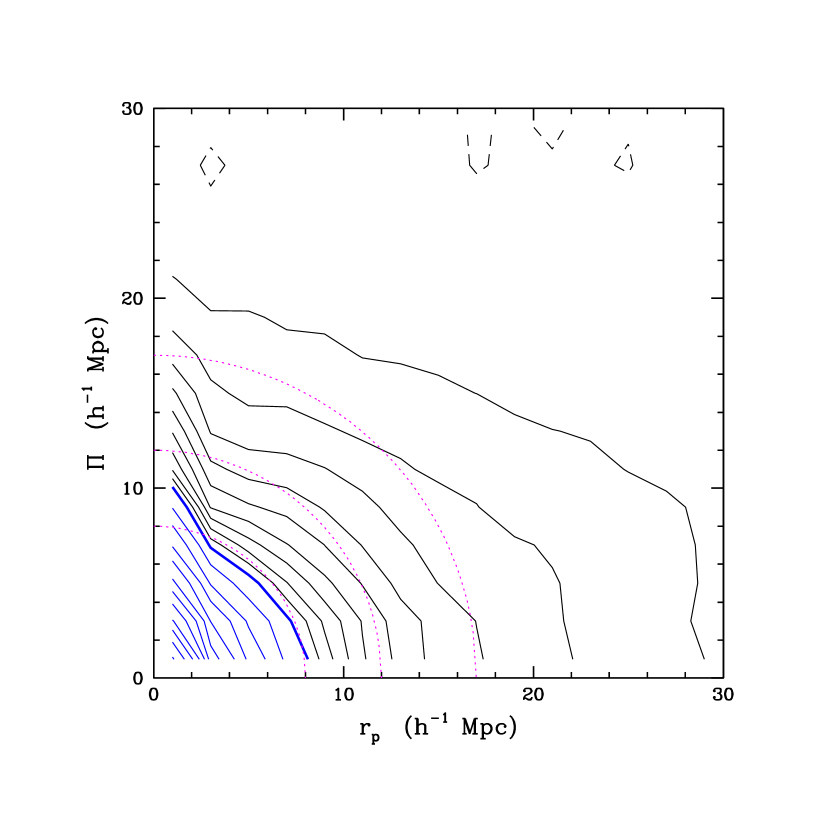
Figure 4: Contours of the galaxy correlation function as a function of tangential separation $r_{p}$ and line-of-sight separation $\pi$, evaluated for the full flux-limited sample in $2\,h^{-1}\;{\rm Mpc}$ bins. The heavy contour marks ${\xi(r_{p},\pi)}=1$; inner contours are spaced by 0.1 in $\log\xi$ and outer contours by 0.1 in $\xi$. The dashed contour marks ${\xi(r_{p},\pi)}=0$. Dotted lines show the isotropic behavior expected in the absence of redshift-space distortions. Contours show the compression at large scales caused by coherent peculiar velocities and the elongation at small $r_{p}$ caused by “finger-of-God” distortions in collapsed structures.

Figure 5 shows ${\xi(r_{p},\pi)}$ separately for red and blue galaxies. The ${g-r}$ galaxy color distribution is bimodal, similar to $u-r$ (Strateva et al., 2001), so we divide the sample at a rest-frame ${g-r}=0.7$, which naturally separates the two populations. The red sample contains roughly twice as many galaxies as the blue one. As expected, the red galaxies exhibit a larger clustering amplitude than do the blue galaxies. The difference in the anisotropy is striking, with the red galaxies exhibiting much stronger finger-of-God distortions on small-scales. Both samples show clear signatures of large scale distortion. We examine the dependence of real space clustering on galaxy color in § 3.3.

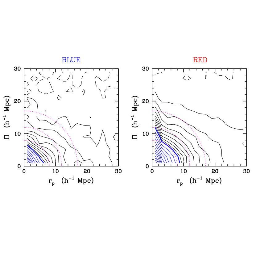
Figure 5: Correlation function contours for galaxies with ${g-r}<0.7$ (left) and ${g-r}>0.7$ (right) in the flux-limited sample. Contour specifications are as in Fig. 4. Red galaxies have a higher amplitude correlation at a given separation, and they show stronger finger-of-God distortions because of their preferential location in dense regions. Both classes of galaxies show large scale compression, though the results for blue galaxies are noisier because of the lower ${\xi(r_{p},\pi)}$ amplitude and smaller sample.

We disentangle the effects of redshift distortions from real space correlations by estimating the projected correlation function ${w_{p}(r_{p})}$ via equation (2), now using logarithmic bins of 0.2 in $r_{p}$. The resulting $w_{p}$ for the full flux-limited sample is shown in Figure 6 together with fits of the data points to a power-law. The fits are done using the measured data points in the range $0.13\,h^{-1}\;{\rm Mpc}<r_{p}<20\,h^{-1}\;{\rm Mpc}$, as this is the range where the measurements are robust. As discussed in §2.2, the power-law fits can be directly related to the real-space correlation function (eq. 4). The inferred real space correlation function is ${\xi(r)}=(r/r_{0})^{-\gamma}$ with $r_{0}=5.59\pm 0.11\,h^{-1}\;{\rm Mpc}$ and $\gamma=1.84\pm 0.01$, when the fit is done using the full covariance matrix (solid line). When using only the diagonal elements (dotted line), i.e., ignoring the correlation of errors between bins, one gets a slightly higher and shallower power-law as the strongly correlated points at large separation are effectively given higher weight when they are treated as independent. The parameters of this diagonal fit are $r_{0}=5.94\pm 0.05\,h^{-1}\;{\rm Mpc}$ and $\gamma=1.79\pm 0.01$, but the errorbars are not meaningful in this case. The power-law provides an approximate description of the projected correlation function, but, as emphasized by Z04, there are notable and systematic deviations from it. The $\chi^{2}/{\rm d.o.f.}$ for the power-law fit when using the jackknife covariance matrix is $\sim 5$. The deviations from a power-law can be naturally explained in the HOD framework as discussed by Z04 and in §4 below. Power-law fits are nonetheless useful as approximate characterizations of the data and for facilitating the comparison to other measurements.

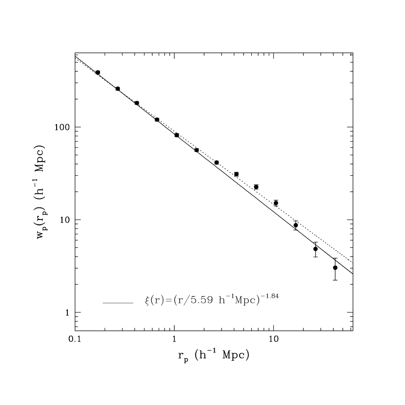
Figure 6: Projected galaxy correlation function ${w_{p}(r_{p})}$ for the flux-limited galaxy sample. The solid line shows a power-law fit to the data points, using the full covariance matrix, which corresponds to a real-space correlation function $\xi(r)=(r/5.59\,h^{-1}\;{\rm Mpc})^{-1.84}$. The dotted line shows the fit when using only the diagonal error elements, corresponding to $\xi(r)=(r/5.94\,h^{-1}\;{\rm Mpc})^{-1.79}$. The fits are performed for $r_{p}<20\,h^{-1}\;{\rm Mpc}$.

Figure 7 shows the real-space correlation function, ${\xi(r)}$, obtained by inverting ${w_{p}(r_{p})}$ for the flux-limited sample using equation (5), independent of the power-law assumption. The lines plotted are the same corresponding power-law fits obtained by fitting ${w_{p}(r_{p})}$. We can see that the characteristic deviation from a power-law is also apparent in ${\xi(r)}$, but we still choose to do all model fitting to ${w_{p}(r_{p})}$ because it is more accurately measured and has better understood errors.

Figure 7: The real-space correlation function ${\xi(r)}$ for the flux-limited galaxy sample, obtained from ${w_{p}(r_{p})}$ as discussed in the text. The solid and dotted lines show the corresponding power-law fits obtained by fitting ${w_{p}(r_{p})}$ using the full covariance matrix or just the diagonal elements, respectively.

3.2 Luminosity Dependence

We examine the clustering dependence on luminosity using sets of volume-limited samples constructed from the full sample, corresponding to different absolute magnitude bins and thresholds. The details of the individual samples are given in Table 1 and Table 2. Figure 8 shows the projected correlation functions obtained for the different volume-limited samples corresponding to galaxies in specified absolute magnitude bins (top-left panel) and to galaxies brighter than the indicated absolute magnitude (top right panel). For clarity, we omit some of the latter subsamples from the plot, but we list their properties in Table 2, and we will use them in § 4. The dependence of clustering on luminosity is clearly evident in Figure 8, with the more luminous galaxies exhibiting higher clustering amplitude. This steady trend holds throughout the luminosity range, confirming the early results of Z02 (but see further discussion below). The slopes of power-law fits to ${w_{p}(r_{p})}$ for the different samples are $\gamma\sim 1.8-2.0$, with a notable steepening for the most luminous bin. These trends are in agreement with an analogous study of the galaxy-mass correlation function from weak lensing measurements in the SDSS (Sheldon et al., 2004).

Table 1: Volume-limited Correlation Function Samples Corresponding to Magnitude Ranges

$M_{r}$	$z$	$N_{\mathrm{gal}}$	${\bar{n}}$	$r_{0}$	$\gamma$	$\frac{\chi^{2}}{d.o.f.}$	$r_{0}^{d}$	$\gamma^{d}$
-23 $-$ -22	$0.10-0.23$	3,499	0.005	10.04 (0.37)	2.04 (0.08)	0.4	10.00 (0.29)	2.04 (0.08)
-22 $-$ -21	$0.07-0.16$	23,930	0.114	6.16 (0.17)	1.85 (0.03)	3.4	6.27 (0.07)	1.86 (0.02)
-21 $-$ -20	$0.04-0.10$	31,053	0.516	5.52 (0.19)	1.78 (0.03)	2.2	5.97 (0.11)	1.77 (0.02)
-21 $-$ -20	$0.04-0.07^{*}$	5,670	0.482	5.02 (0.30)	1.80 (0.05)	1.1	4.96 (0.16)	1.86 (0.03)
-20 $-$ -19	$0.03-0.07$	14,223	0.850	4.41 (0.23)	1.87 (0.04)	1.9	4.74 (0.11)	1.85 (0.03)
-19 $-$ -18	$0.02-0.04$	4,545	1.014	3.51 (0.32)	1.92 (0.05)	0.9	3.77 (0.17)	1.89 (0.06)
-18 $-$ -17	$0.01-0.03$	1,950	1.209	2.68 (0.39)	1.99 (0.09)	0.3	2.83 (0.19)	1.94 (0.11)

Note. — All samples use $14.5<r\lesssim 17.77$. ${\bar{n}}$ is measured in units of $10^{-2}$ $h^{3}$ Mpc^-3. $r_{0}$ and $\gamma$ are obtained from a fit for $w_{p}(r_{p})$ using the full error covariance matrix. ${r_{0}}^{d}$ and ${\gamma}^{d}$ are the corresponding values when using just the diagonal elements. Values in brackets are the fitting error. The clipped $-21<M_{r}<-20$ sample, indicated with a ^∗, is confined to a limiting redshift $z_{\rm max}=0.07$ to avoid the effects of the large supercluster at $z=0.08$ (see text).

Table 2: Volume-limited Correlation Function Samples Corresponding to Magnitude Thresholds

${M_{r}}^{\mathrm{max}}$	$z^{\mathrm{max}}$	$N_{\mathrm{gal}}$	${\bar{n}}$	$r_{0}$	$\gamma$	$\frac{\chi^{2}}{d.o.f.}$	$r_{0}^{d}$	$\gamma^{d}$
-22.0	0.22	3,626	0.006	9.81 (0.39)	1.97 (0.08)	0.8	9.81 (0.30)	1.97 (0.08)
-21.5	0.19	11,712	0.031	7.70 (0.22)	1.88 (0.03)	1.7	7.77 (0.12)	1.88 (0.02)
-21.0	0.15	26,015	0.117	6.24 (0.16)	1.90 (0.02)	4.0	6.49 (0.08)	1.89 (0.02)
-20.5	0.13	36,870	0.308	5.81 (0.15)	1.88 (0.02)	1.6	5.98 (0.07)	1.86 (0.02)
-20.0	0.10	40,660	0.611	5.58 (0.20)	1.83 (0.03)	2.8	6.12 (0.11)	1.81 (0.02)
-20.0	0.06∗	9,161	0.574	5.02 (0.24)	1.88 (0.04)	0.8	5.09 (0.13)	1.90 (0.03)
-19.5	0.08	35,854	1.015	4.86 (0.17)	1.85 (0.02)	2.0	5.19 (0.10)	1.85 (0.02)
-19.0	0.06	23,560	1.507	4.56 (0.23)	1.89 (0.03)	1.7	4.85 (0.11)	1.88 (0.03)
-18.5	0.05	14,244	2.060	3.91 (0.27)	1.90 (0.05)	1.0	4.37 (0.15)	1.92 (0.04)
-18.0	0.04	8,730	2.692	3.72 (0.30)	1.87 (0.05)	1.9	4.39 (0.20)	1.84 (0.06)

Note. — All samples use $10.0<r<17.5$. $z^{\mathrm{min}}$ for the samples is $0.02$. ${\bar{n}}$ is measured in units of $10^{-2}$ $h^{3}$ Mpc^-3. $r_{0}$ and $\gamma$ are obtained from a fit for $w_{p}(r_{p})$ using the full error covariance matrix. ${r_{0}}^{d}$ and ${\gamma}^{d}$ are the corresponding values when using just the diagonal elements. Values in brackets are the fitting errors. The clipped $M_{r}<-20$ sample, indicated with a ^∗, is confined to a limiting redshift $z_{\rm max}=0.06$ to avoid the effects of the large supercluster at $z=0.08$ (see text).

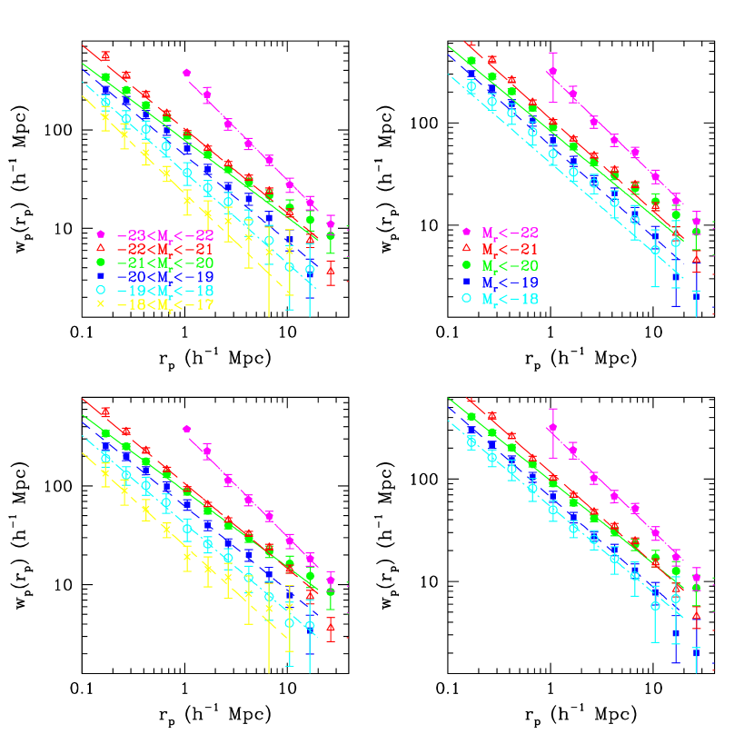
Figure 8: Top left: Projected galaxy correlation functions ${w_{p}(r_{p})}$ for volume-limited samples with the indicated absolute magnitude and redshift ranges. Lines show power-law fits to each set of data points, using the full covariance matrix. Top right: Same as top left, but now the samples contain all galaxies brighter than the indicated absolute magnitude, i.e., they are defined by luminosity thresholds rather than luminosity ranges. Bottom panels: Same as the top panels, but now with power-law fits that use only the diagonal elements of the covariance matrix.

The lines plotted in the top panels are power-law fits to the measurements obtained using the full error covariance matrix. The fitted values of $r_{0}$ and $\gamma$ are specified in Tables 1 and 2. Note that some of the fits, particularly for the smaller volume subsamples, lie systematically below the data points. While initially counter-intuitive, these fits do indeed have lower $\chi^{2}$ than higher amplitude power-laws that pass closer to the points. This kind of behavior is not uncommon when fitting strongly correlated data points, and in tests with the PTHalo mock catalogs on some small volume samples we find similar results using mock catalog covariance matrices in place of jackknife covariance matrices. We thus have no reason to think that these are not the “best” values of $r_{0}$ and $\gamma$, in a statistical sense. However, the covariance matrices do have noise because they are estimated from the finite data samples themselves. For good measure, the bottom panels in Figure 8 show the same measurements, but now with fits using only the diagonal components of the jackknife covariance matrix. These fits pass through the points in agreement with the “chi-by-eye” expectation. The best-fitting values of $r_{0}$ and $\gamma$ for these cases are quoted in the tables, but the $\chi^{2}$ values are no longer meaningful as goodness-of-fit estimates.

The $-21<M_{r}<-20$ luminosity-bin sample and the $M_{r}<-20$ luminosity-threshold sample in Figure 8 exhibit anomalously high ${w_{p}(r_{p})}$ at large separations, with a flat slope at $r_{p}\gtrsim 3\,h^{-1}\;{\rm Mpc}$ that is clearly out of line with other samples. We believe that this anomalous behavior is a “cosmic variance” effect caused by an enormous supercluster at $z\sim 0.08$, slightly inside the limiting redshift $z_{\rm max}=0.10$ of these two samples. This “Sloan Great Wall” at $\alpha\sim 200^{\circ}$, $\delta\sim 0^{\circ}$ is the largest structure detected in the SDSS to date, or, indeed, in any galaxy redshift survey (see Gott et al. 2005). It has an important effect on the $z_{\rm max}=0.1$ samples, but no effect on the fainter samples, which have $z_{\rm max}<0.08$, and little effect on brighter samples, which cover a substantially larger volume. If we repeat our analysis excluding the supercluster region in an ad hoc fashion, then the large scale ${w_{p}(r_{p})}$ amplitude drops for these two $z_{\rm max}=0.10$ samples but changes negligibly for other samples. Because our jackknife subsamples are smaller than the supercluster, the jackknife errorbars do not properly capture the large variance introduced by this structure. We note that while this super-cluster is certainly a striking feature in the data, its existence is in no contradiction to concordance cosmology: preliminary tests with the PTHalo mock catalogs reveal similar structures in more than $10\%$ of the cases.

A more general cosmic variance problem is that we measure the clustering of each galaxy luminosity subset over a different volume, and variations in the true underlying structure could masquerade as luminosity dependence of galaxy bias. To test for this problem, we compare the ${w_{p}(r_{p})}$ measurements for each pair of adjacent luminosity bins to the values measured when we restrict the two samples to the volume where they overlap (and thus trace identical underlying structure; see the corresponding redshift ranges in Table 1). In each panel of Figure 9, the points show our standard ${w_{p}(r_{p})}$ measurement for the maximum volume accessible to each luminosity bin; brighter and fainter luminosity bins are represented by open and filled circles, respectively. The dashed and solid curves and errorbars show the corresponding measurements when the samples are restricted to the volume where they overlap. In the absence of any cosmic variance, the dashed curve should pass through the open points and the solid curve through the filled points. This is essentially what we see for the two faintest bins, shown in the lower right, except for a low significance fluctuation at large scales in the overlap measurement for $-20<M_{r}<-19$.

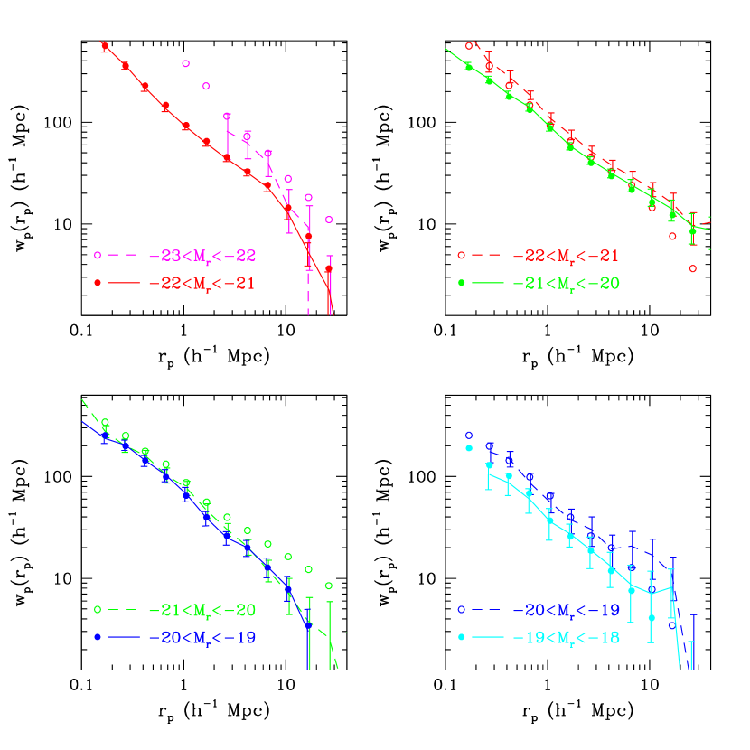
Figure 9: The impact of finite volume fluctuations on the measured luminosity dependence of ${w_{p}(r_{p})}$. Each panel compares the projected correlation function of two neighboring absolute-magnitude bins. The filled and open symbols show the results using the maximum accessible redshift range for each bin, as in Fig. 8. Lines show the measurements of ${w_{p}(r_{p})}$ restricted to the overlap redshift range in which both sets of galaxies are observable. Error bars, attached to the lines (not the points), represent $1\sigma$ errors for these smaller, overlap samples.

Moving to the next comparison in the lower left, we see the dramatic effect of the $z\sim 0.08$ supercluster. When the $-21<M_{r}<-20$ sample is restricted to the overlap volume, reducing $z_{\rm max}$ from 0.10 to 0.07, its projected correlation function drops and steepens, coming into good agreement with that of the $-20<M_{r}<-19$ sample. Conversely, when the $-22<M_{r}<-21$ sample is restricted to $z_{\rm max}=0.1$ (dashed curve, upper right), it acquires an anomalous large separation tail like that of the (full) $-21<M_{r}<-20$ sample. Increasing the minimum redshift of this sample to $z_{\rm min}=0.10$ (solid curve, upper left), on the other hand, has minimal impact, suggesting that the influence of the supercluster is small for the full $-22<M_{r}<-21$ sample, which extends from $z_{\rm min}=0.07$ to $z_{\rm max}=0.16$. The large scale amplitude of the $-23<M_{r}<-22$ sample drops when it is restricted to $z_{\rm max}=0.16$, but this drop again has low significance because of the limited overlap volume, which contains only about 1000 galaxies in this luminosity range. In similar fashion, the overlap between the $-19<M_{r}<-18$ and $-18<M_{r}<-17$ volumes is too small to allow a useful cosmic variance test for our faintest sample. We have carried out the volume overlap test for the luminosity-threshold samples in Table 2, and we reach a similar conclusion to that for the luminosity bins: the $M_{r}<-20$ sample, with $z_{\rm max}=0.10$, is severely affected by the $z\sim 0.08$ supercluster, but other samples appear robust to changes in sample volume.

Given these results, we have chosen to use the measurements from the $-21<M_{r}<-20$ sample limited to $z_{\rm max}=0.07$ (the same limiting redshift as for $-20<M_{r}<-19$) and the $M_{r}<-20$ sample limited to $z_{\rm max}=0.06$ (same as $M_{r}<-19$) in our subsequent analyses. We list properties of these reduced samples in Tables 1 and 2. This kind of data editing should become unnecessary as the SDSS grows in size, and even structures as large as the Sloan Great Wall are represented with their statistically expected frequency. As an additional test of cosmic variance effects, we have measured ${w_{p}(r_{p})}$ separately in each of the three main angular regions of the survey (see Figure 1), and despite significant fluctuations from region to region, we find the same continuous trend of clustering strength with luminosity in each case.

Figure 10 presents the luminosity dependence in the form of relative bias functions, $b_{\rm rel}(r_{p})\equiv[{w_{p}(r_{p})}/w_{p,{\rm fid}}(r_{p})]^{1/2},$ where ${w_{p}(r_{p})}$ is the measured result for a luminosity bin and $w_{p,{\rm fid}}(r_{p})$ is the projected correlation function corresponding to $\xi(r)=(r/5.0\,h^{-1}\;{\rm Mpc})^{-1.8}$. We take a power-law rather than a given sample as our fiducial so that measurement noise does not propagate into the definition of bias functions. The bias factors increase steadily with luminosity, and they are roughly scale independent, with $\sim 10-20\%$ fluctuations, for all samples except the brightest one. The $-23<M_{r}<-22$ galaxies have a ${w_{p}(r_{p})}$ slope steeper than $-1.8$, so their bias relative to fainter galaxies increases with decreasing $r_{p}$.

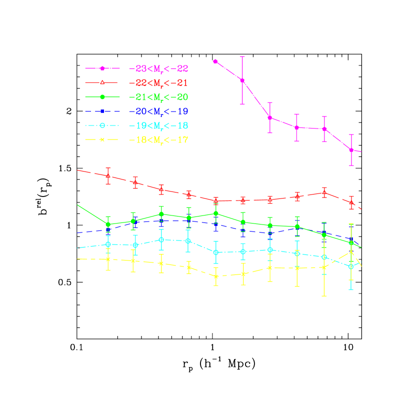
Figure 10: Relative bias factors as a function of separation $r_{p}$ for samples defined by luminosity ranges. Bias factors are defined by $b_{\rm rel}(r_{p})\equiv[{w_{p}(r_{p})}/w_{p,{\rm fid}}(r_{p})]^{1/2}$ relative to a fiducial power-law corresponding to ${\xi(r)}=(r/5\,h^{-1}\;{\rm Mpc})^{-1.8}$.

To summarize our results and compare to previous work, we take the bias factors at $r_{p}=2.7\,h^{-1}\;{\rm Mpc}$ and divide them by the bias factor $b_{*}$ of the $-21<M_{r}<-20$ sample, which has luminosity $L\approx L_{*}$. We choose $2.7\,h^{-1}\;{\rm Mpc}$ because it is out of the extremely nonlinear regime and all samples are well measured there; one can see from Figure 10 that other choices would give similar but not identical results. Figure 11 plots $b/b_{*}$ vs. $\log L/L_{*}$, where the solid points show the results from our ${w_{p}(r_{p})}$ measurements. The dashed curve is the fit to SDSS results by Tegmark et al. (2004a), where bias factors are derived from the galaxy power spectrum at wavelengths $2\pi/k\sim 100\,h^{-1}\;{\rm Mpc}$, in the linear (or at least near-linear) regime. The ${w_{p}(r_{p})}$ and $P(k)$ results agree remarkably well, despite being measured at very different scales. The dotted curve in Figure 11 shows the fit of Norberg et al. (2001), based on ${w_{p}(r_{p})}$ measurements of galaxies with $\log L/L_{*}>-0.7$ in the 2dFGRS. Agreement is again very good, over the range of the Norberg et al. (2001) measurements, with all three relative bias measurements (from two independent data sets) showing that the bias factor increases sharply for $L>L_{*}$, as originally argued by Hamilton (1988). At luminosities $L\lesssim 0.2L_{*}$, the Tegmark et al. (2004a) formula provides a better fit to our data than the extrapolation of the Norberg et al. (2001) formula.

Figure 11: Relative bias factors for samples defined by luminosity ranges. Bias factors are defined by the relative amplitude of the ${w_{p}(r_{p})}$ estimates at a fixed separation of $r_{p}=2.7\,h^{-1}\;{\rm Mpc}$ and are normalized by the $-21<M_{r}<-20$ sample ($L\approx L_{*}$). The dashed curve is a fit obtained from measurements of the SDSS power spectrum, $b/b_{*}=0.85+0.15L/L_{*}-0.04(M-M_{*})$ (Tegmark et al., 2004a), and the dotted curve is a fit to similar ${w_{p}(r_{p})}$ measurements in the 2dF survey, $b/b_{*}=0.85+0.15L/L_{*}$ (Norberg et al., 2001).

3.3 Color Dependence

In addition to luminosity, the clustering of galaxies is known to depend on color, spectral type, morphology, and surface brightness. These quantities are strongly correlated with each other, and in Z02 we found that dividing galaxy samples based on any of these properties produces similar changes to ${w_{p}(r_{p})}$. This result holds true for the much larger sample investigated here. For this paper, we have elected to focus on color, since it is more precisely measured by the SDSS data than the other quantities. In addition, Blanton et al. (2005a) find that luminosity and color are the two properties most predictive of local density, and that any residual dependence on morphology or surface brightness at fixed luminosity and color is weak.

Figure 12 shows a color-magnitude diagram constructed from a random subsampling of the volume-limited samples used in our analysis. The gradient along each magnitude bin reflects the fact that in each volume faint galaxies are more common than bright ones, while the offset from bin to bin reflects the larger volume sampled by the brighter bins. While we used $g-r=0.7$ for the color division of the flux-limited sample (Fig. 5), in this section we adopt the tilted color cut shown in Figure 12, which better separates the E/S0 ridgeline from the rest of the population. It has the further advantage of keeping the red:blue ratio closer to unity in our different luminosity bins, though it remains the case that red galaxies predominate in bright bins and blue galaxies in faint ones (with roughly equal numbers for the $L_{*}$ bin). The dependence of the color separation on luminosity has been investigated more quantitatively by Baldry et al. (2004).

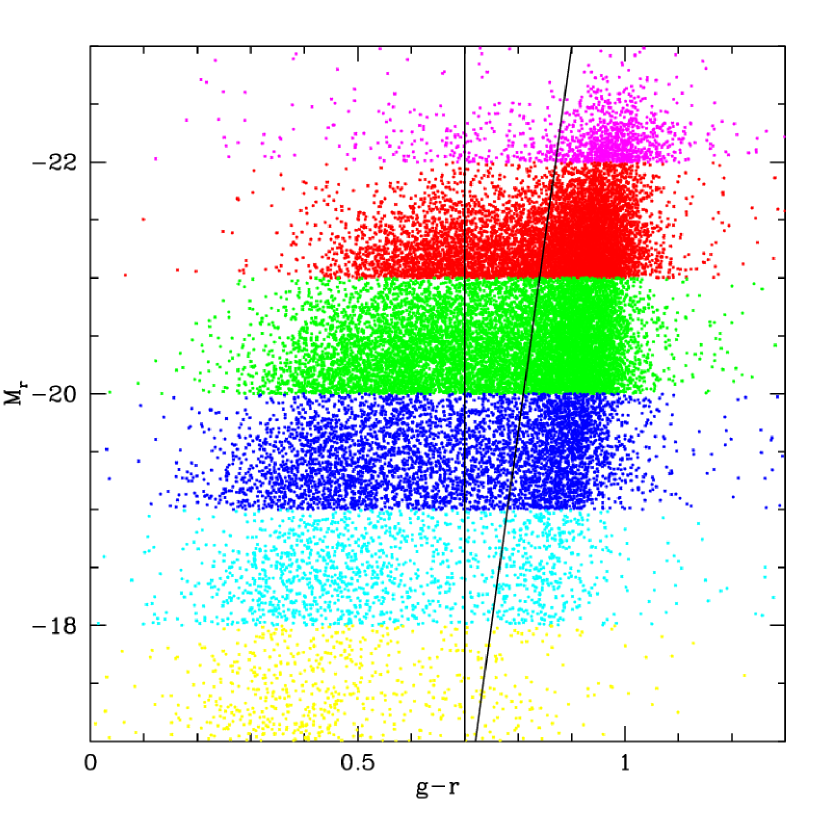
Figure 12: K-corrected ${g-r}$ color vs. absolute magnitude for all galaxies comprising our volume-limited luminosity bins samples. A clear color-magnitude trend is evident. The vertical line demarcates a simple cut at ${g-r}=0.7$, while the tilted line indicates the luminosity-dependent color cut that we adopt for the analyses in §§3.3 and 4.3.

Figure 13 shows, as a representative case, the projected correlation function obtained with the tilted color division for the $-20<M_{r}<-19$ volume-limited sample. The red galaxy ${w_{p}(r_{p})}$ has a steeper slope and a higher amplitude at all $r_{p}\lesssim 10\,h^{-1}\;{\rm Mpc}$; at $r_{p}>10\,h^{-1}\;{\rm Mpc}$ the two correlation functions are consistent within the (large) statistical errors. Power-law fits for these samples using the full covariance matrix give $r_{0}=5.7\,h^{-1}\;{\rm Mpc}$ and $\gamma=2.1$ for the red sample, and $r_{0}=3.6\,h^{-1}\;{\rm Mpc}$ and $\gamma=1.7$ for the blue sample. The change in slope contrasts with the results for the luminosity dependence, where (with small variations) the slope remains fairly constant and only the clustering amplitude changes. The results for the color dependence in the other luminosity bins, and in luminosity-threshold samples and the flux-limited sample, are qualitatively similar (see Figures 22 and 23 below). The behavior in Figure 13 is strikingly similar to that found by Madgwick et al. (2003, Fig. 2) for flux-limited samples of active and passive galaxies in the 2dFGRS, where spectroscopic properties are used to distinguish galaxies with ongoing star formation from those without.

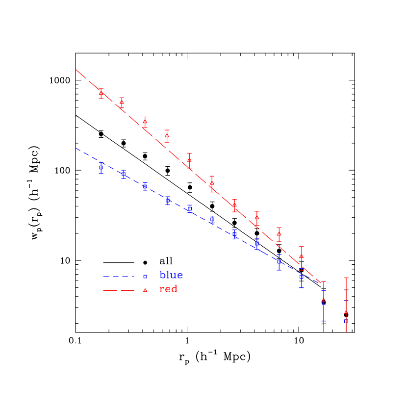
Figure 13: Projected correlation function of the full volume-limited sample of all galaxies with $-20<M_{r}<-19$ and of the blue and red galaxies in this sample, with the color cut indicated by the tilted line in Fig. 12. Lines show the best-fit power-laws.

Figure 14 shows the luminosity dependence of ${w_{p}(r_{p})}$ separately for blue galaxies (middle panel) and red galaxies (bottom panel). We divide ${w_{p}(r_{p})}$ by a fiducial power-law corresponding to $\xi(r)=(r/5.0\,h^{-1}\;{\rm Mpc})^{-1.8}$, and we show the luminosity dependence for the full (red and blue) samples again in the top panel (repeating Fig. 10, but here showing $b^{2}$ instead of $b$). We focus on the four central luminosity bins, since the $-18<M_{r}<-17$ sample is too small once it is divided by color, and the $-23<M_{r}<-22$ sample consists mainly of red galaxies alone. Blue galaxies exhibit a roughly scale-independent luminosity dependence reminiscent of the full sample, but even the most luminous blue galaxy bin only has $r_{0}\approx 5\,h^{-1}\;{\rm Mpc}$. The red galaxies are always more clustered than the fiducial power-law on small scales, regardless of luminosity, and the luminosity dependence for red galaxies is more complex. At large scales, the luminous red galaxies are the most strongly clustered, but at small scales faint red galaxies have the highest and steepest correlation function, with ${w_{p}(r_{p})}$ of all samples intersecting at $r_{p}\sim 1\,h^{-1}\;{\rm Mpc}$. All of these trends would also hold if we adopted a fixed color cut at $g-r=0.7$ instead of the tilted color cut used in this section.

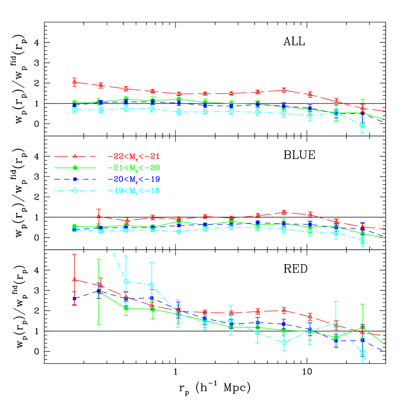
Figure 14: Luminosity and color dependence of the galaxy correlation function. Upper, middle, and lower panels show projected correlation functions of all galaxies, blue galaxies, and red galaxies, respectively, in the indicated absolute-magnitude ranges. All projected correlation functions are divided by a fiducial power-law corresponding to $\xi(r)=(r/5\,h^{-1}\;{\rm Mpc})^{-1.8}$.

Figure 14 demonstrates that the luminosity and color dependence of the galaxy correlation function is not trivially separable, nor is the luminosity dependence a simple consequence of the color dependence (or vice versa). The effect of color is in some sense stronger, since red galaxies of any luminosity are more clustered than blue galaxies of any luminosity (at least for $r_{p}\lesssim 3\,h^{-1}\;{\rm Mpc}$). However, luminosity dependence of clustering remains evident within the red and blue populations separately. The overall appearance of Figure 14 is roughly like that of Figure 7 of Norberg et al. (2002), who divide their samples into early and late spectral types, but we find systematically different slopes for red and blue galaxies, a steadier luminosity trend for blue galaxies, and a much more noticeable scale dependence of relative bias for red galaxies. These differences could reflect the difference in the sample definitions (color versus spectral type) and overall selection ($r$-band versus $b_{J}$-band). The strong small scale clustering of faint red galaxies in our sample agrees with the results for faint early type galaxies in Norberg et al. (2002), and with the results of Hogg et al. (2003), who find that these galaxies reside in denser environments than red galaxies of intermediate luminosity. Kayo et al. (2004) find qualitatively similar trends for the dependence of the redshift-space two-point correlation amplitude on luminosity, color, and morphological type.

4 HOD Modeling of the SDSS Galaxy Clustering

4.1 HOD Framework and Formalism

We now turn to physical interpretation of these results using the Halo Occupation Distribution (HOD) framework, which describes the bias between galaxies and mass in terms of the probability distribution $P(N|M)$ that a halo of virial mass $M$ contains $N$ galaxies of a given type, together with prescriptions for the relative bias of galaxies and dark matter within virialized halos. Because the real-space correlation function describes a limited (but important) subset of the information encoded in galaxy clustering, we will have to fit restricted HOD models with a small number of free parameters, and we will assume that the underlying cosmological model is known a priori. However, relative to power-law fits, HOD modeling fits the data more accurately (in most cases) and in a way that we consider more physically informative. In the longer run, constraints from multiple galaxy clustering statistics can be combined to test the HOD predictions of galaxy formation models (e.g., Kauffmann, Nusser, & Steinmetz 1997; Kauffman et al. 1999; Benson et al. 2000; Somerville et al. 2001; Yoshikawa et al. 2001; White, Hernquist, & Springel 2001; Berlind et al. 2003; Kravtsov et al. 2004), and to obtain simultaneous constraints on cosmological parameters (see discussions by Berlind & Weinberg 2002; Zheng et al. 2002; Weinberg 2002; van den Bosch, Mo, & Yang 2003b; Z. Zheng & D. Weinberg 2005, in preparation; and an initial application to SDSS data by Abazajian et al. 2005).

We assume a spatially flat $\Lambda$CDM cosmological model with matter density parameter $\Omega_{m}=0.3$. For the matter fluctuation power spectrum, we adopt the parameterization of Efstathiou, Bond, & White (1992) and assume that the spectral index of the inflationary power spectrum is $n_{s}=1$, the rms matter fluctuation (linearly evolved to $z=0$) at a scale of 8$h^{-1}{\rm Mpc}$ is $\sigma_{8}=0.9$, and the shape parameter is $\Gamma=0.21$. These parameters are in good agreement with joint analyses of CMB anisotropies and the 2dFGRS or SDSS galaxy power spectrum (Percival et al., 2003; Spergel et al., 2003; Tegmark et al., 2004b) or with a more recent analysis that incorporates constraints from the SDSS Ly$\alpha$ forest and galaxy-galaxy lensing (Seljak et al., 2004b). We have verified that our results do not change significantly if we use CMBFAST (Seljak & Zaldarriaga, 1996) to compute the linear theory power spectrum instead of the Efstathiou, Bond, & White (1992) form.

We focus first on luminosity-threshold samples, mainly because the theoretical predictions for HODs have been studied more extensively for samples defined by mass or luminosity thresholds (e.g., Seljak 2000; White, Hernquist, & Springel 2001; Yoshikawa et al. 2001; Berlind et al. 2003; Kravtsov et al. 2004; Zheng 2004). The larger galaxy numbers in luminosity-threshold samples also allow higher precision ${w_{p}(r_{p})}$ measurements. Our adopted HOD parameterization is motivated by Kravtsov et al.’s (2004) recent work on substructures in high-resolution dissipationless simulations. They find that when the HOD is divided into contributions of central and satellite objects, it assumes a simple form. For a subhalo sample above a threshold in maximum circular velocity (known empirically to correlate with luminosity), the mean occupation number for central substructures can be modeled as a step function, i.e., $\langle N_{\rm cen}\rangle=1$ for halos with mass $M\geq M_{\rm min}$ and $\langle N_{\rm cen}\rangle=0$ for $M<M_{\rm min}$, while the distribution of satellite substructures can be well approximated by a Poisson distribution with the mean following a power-law, $\langle N_{\rm sat}\rangle=(M/M_{1})^{\alpha}$, with $\alpha\approx 1$. This way of separating central and satellite substructures naturally explains both the general shape of the mean occupation function $\langle N\rangle_{M}$ and, more importantly, the transition from sub-Poisson fluctuations at low occupation number to Poisson fluctuations at high occupation number found in semi-analytic and numerical galaxy formation models (e.g., Benson et al. 2000; Berlind et al. 2003). Zheng et al. (2004) show that the Kravtsov et al. (2004) formulation also provides a good description of results from the semi-analytic models and hydrodynamic simulations.

As implemented here, this HOD formulation has three free parameters: $M_{\rm min}$, the minimum halo mass for galaxies above the luminosity threshold, $M_{1}$, the mass of a halo that on average hosts one satellite galaxy above the threshold, and $\alpha$, the power-law slope of the satellite mean occupation function. One of these, which we take to be $M_{\rm min}$, is fixed by matching the observed space density of the sample, leaving $M_{1}$ and $\alpha$ as free parameters to fit $w_{p}(r_{p})$. This parameterization thus has the same number of adjustable degrees of freedom as an ($r_{0}$, $\gamma$) power-law, allowing a fair comparison of goodness of fit. However, this parameterization is not a unique choice (we discuss some variations below), and achieving a fully accurate fit to the predictions of galaxy formation models requires additional parameters to describe the shapes of the low mass cutoff for central and satellite galaxies. The HOD parameterization adopted in Z04, with the mean occupation function changing from a plateau of $\langle N\rangle_{M}=1$ to a power-law above a given halo mass, can be regarded as a simplified version of the one used in this paper.

In halo-based calculations, the two-point correlation function $\xi(r)$ is decomposed into two components (see, e.g., Zheng 2004),

$$\xi(r)=[1+\xi_{\rm 1h}(r)]+\xi_{\rm 2h}(r),$$ (7)

where the one-halo term $\xi_{\rm 1h}(r)$ (dominant at small scales) and the two-halo term $\xi_{\rm 2h}(r)$ (dominant at large scales) represent contributions by galaxy pairs from the same halos and from different halos, respectively. The “1+” in equation (7) arises because the total number of pairs (proportional to $1+\xi$) is the sum of the number of one-halo and two-halo pairs (proportional to $1+\xi_{\rm 1h}$ and $1+\xi_{\rm 2h}$). Our computations of these two terms follow those in Z04 and Zheng (2004), as briefly reviewed below.

We calculate the one-halo term in real space through (e.g., Berlind & Weinberg 2002)

$$1+\xi_{\rm 1h}(r)=\frac{1}{2\pi r^{2}\bar{n}_{g}^{2}}\int_{0}^{\infty}dM\frac{dn}{dM}\frac{\langle N(N-1)\rangle_{M}}{2}\frac{1}{2R_{\rm vir}(M)}F^{\prime}\left(\frac{r}{2R_{\rm vir}}\right),$$ (8)

where $\bar{n}_{g}$ is the mean number density of galaxies of the given sample, $dn/dM$ is the halo mass function (Sheth & Tormen 1999; Jenkins et al. 2001), $\langle N(N-1)\rangle_{M}/2$ is the average number of galaxy pairs in a halo of mass $M$, and $F(r/2R_{\rm vir})$ is the cumulative radial distribution of galaxy pairs. For luminosity-threshold samples, one galaxy is always assumed to reside at the center of a halo. With the separation of central and satellite galaxies, $F^{\prime}(x)$ is then the pair-number weighted average of the central-satellite pair distribution $F^{\prime}_{\rm cs}(x)$ and the satellite-satellite pair distribution $F^{\prime}_{\rm ss}(x)$ (see, e.g., Berlind & Weinberg 2002; Yang, Mo, & van den Bosch 2003),

$$\frac{\langle N(N-1)\rangle_{M}}{2}F^{\prime}(x)=\langle N_{\rm cen}N_{\rm sat}\rangle_{M}F^{\prime}_{\rm cs}(x)+\frac{\langle N_{\rm sat}(N_{\rm sat}-1)\rangle_{M}}{2}F^{\prime}_{\rm ss}(x).$$ (9)

For our parameterization, the occupation number of satellite galaxies follows a Poisson distribution, which implies that $\langle N_{\rm sat}(N_{\rm sat}-1)\rangle=\langle N_{\rm sat}\rangle^{2}$. In cases where we allow a smooth cutoff in $N_{\rm cen}$, we further assume that $\langle N_{\rm cen}N_{\rm sat}\rangle_{M}=\langle N_{\rm cen}\rangle_{M}\langle N_{\rm sat}\rangle_{M}$, but $N_{\rm sat}\ll 1$ when $N_{\rm cen}$ is significantly below one in any case. The central-satellite galaxy pair distribution, $F^{\prime}_{\rm cs}(x)$, is just the normalized radial distribution of galaxies. In this paper, we assume that the satellite galaxy distribution follows the dark matter distribution within the halo, which we describe by a spherically symmetric NFW profile (Navarro, Frenk, & White 1995, 1996, 1997) truncated at the virial radius (defined to enclose a mean overdensity of 200). The satellite-satellite galaxy pair distribution $F^{\prime}_{\rm ss}(x)$ is then the convolution of the NFW profile with itself (see Sheth et al. 2001). For the dependence of NFW halo concentration on halo mass, we use the relation given by Bullock et al. (2001), after modifying it to be consistent with our slightly different definition of the halo virial radius.

On large scales, the two-halo term is a weighted average of halo correlation functions, where the weight is proportional to the halo number density times the mean galaxy occupation. On intermediate scales, one must also convolve with the finite halo size, and it is easier to do the calculation in Fourier space and transform it to obtain the real space correlation function. To achieve the accuracy needed to model the SDSS data, we improve upon the original calculations of Seljak (2000) and Scoccimarro et al. (2001) by taking into account the nonlinear evolution of matter clustering (Smith et al., 2003), halo exclusion, and the scale-dependence of the halo bias factor (see Z04 and Zheng 2004 for details).

We project $\xi(r)$ to obtain $w_{p}(r_{p})$ using the first part of equation (3) and setting $r_{\rm max}=40h^{-1}{\rm Mpc}$. Under the plane-parallel approximation, for an ideal case where $r_{\rm max}\rightarrow\infty$, the projected correlation function is not affected at all by redshift space distortion. However, since the measured $w_{p}(r_{p})$ is derived from a finite projection out to $r_{\rm max}$, redshift distortion cannot be completely eliminated, especially at large $r_{p}$. We have verified that increasing both $\pi_{\rm max}$ in the measurement and $r_{\rm max}$ in the HOD modeling to $80h^{-1}{\rm Mpc}$ has almost no effect on the inferred HOD. Still, we choose to only fit data points with $r_{p}<20h^{-1}{\rm Mpc}$ to avoid any possible contamination by redshift space distortion. When fitting and evaluating $\chi^{2}$, we use the full jackknife covariance matrix.

4.2 Modeling the Luminosity Dependence

As discussed in § 3.2, the Sloan Great Wall produces an anomalous high amplitude tail at large $r_{p}$ for the $M_{r}<-20$ sample with $z_{\rm max}=0.10$, and we therefore use $z_{\rm max}=0.06$ to get a more reliable estimate of ${w_{p}(r_{p})}$ for this luminosity threshold. Figure 15 shows fits to $w_{p}(r_{p})$ for $M_{r}<-20$ samples with $z_{\rm max}=0.10$ and 0.06, with the mean occupation function $\langle N\rangle_{M}$ shown in the right-hand panel and the predicted and observed $w_{p}(r_{p})$ in the left-hand panel. The quality of fit is much better for the shallower sample ($\chi^{2}/{\rm d.o.f.}=0.68$ vs. $1.65$), but the fit parameters are nearly identical. Given the underlying matter correlation function of the adopted cosmology and the requirement of matching the observed number density, there is simply not much freedom to increase the large-scale values of ${w_{p}(r_{p})}$ while remaining consistent with the data at $r_{p}\lesssim 3h^{-1}{\rm Mpc}$, where the one-halo contribution is important. Our derived HOD parameters (though not the $\chi^{2}$ values) are thus relatively insensitive to statistical fluctuations or systematic uncertainties in $w_{p}(r_{p})$ at $r_{p}\gtrsim 5h^{-1}{\rm Mpc}$, where the difference in $w_{p}(r_{p})$ is largest. The HOD parameters are similarly insensitive to the choice of halo bias factors. We generally adopt the formula of Sheth, Mo, & Tormen (2001) for halo bias as a function of mass, since we have tuned our treatment of halo exclusion and the scale dependence of halo bias assuming these results. If we instead use the formula of Seljak & Warren (2004) (with the same treatment of exclusion and scale dependence), then we find negligible change in the best-fit HODs, but the predicted amplitude of ${w_{p}(r_{p})}$ at large scales is generally lower, increasing $\chi^{2}$ for some samples and decreasing it for others.

Figure 15: HOD fits to the projected correlation function of the $M_{r}<-20$ sample, which has the greatest sensitivity to limiting redshift (Fig. 9). In the left panel, open circles show the measured $w_{p}(r_{p})$ for $z_{\rm max}=0.10$, and the dashed curve shows the predicted $w_{p}(r_{p})$ for the best-fit HOD model, whose mean occupation function is shown by the dashed curve in the right panel. Filled circles show the measured $w_{p}(r_{p})$ for $z_{\rm max}=0.06$, the same cutoff used for the $M_{r}<-19$ sample. Solid curves show the mean occupation function (right panel) and predicted $w_{p}(r_{p})$ (left panel) from fitting these data points. Values of $\chi^{2}/{\rm d.o.f.}$ for the best-fit power-laws and HOD models are listed in the right panel. Reducing $z_{\rm max}$ eliminates the anomalous high amplitude tail of $w_{p}(r_{p})$ at large $r_{p}$, thereby greatly improving the statistical quality of the HOD (and power-law) fit, but it has little effect on the values of the best-fit HOD parameters.

Figure 16 shows HOD fits to the projected correlation functions of samples of different luminosity thresholds. Table 3 lists the HOD parameters and $\chi^{2}$ values for HOD and power-law fits to these samples. With the same number of degrees of freedom, HOD modeling generally yields a better fit than a power-law correlation function. The brightest sample is a strong exception, which we will discuss below. The two faintest samples are mild exceptions, but the small volume probed by these samples makes their overall normalization somewhat uncertain, perhaps by an amount that exceeds the internal jackknife error estimates. The $M_{r}<-21$ correlation function has a marked inflection at $r_{p}\sim 2h^{-1}{\rm Mpc}$. Z04 showed that this feature is naturally explained in the HOD framework by the transition near the virial diameter of large halos from the steeply falling one-halo term dominant at smaller scales to the flatter two-halo term dominant at larger scales (see their Figs. 2 and 3). Figure 17 plots the $w_{p}(r_{p})$ data and the HOD fits divided by an $r_{p}^{-0.8}$ power-law. While the power-law departures are not as striking for less luminous samples, nearly all of them show some change in slope at $r_{p}\sim 2h^{-1}{\rm Mpc}$, as the HOD fits generally predict, lending further support to the results of Z04.

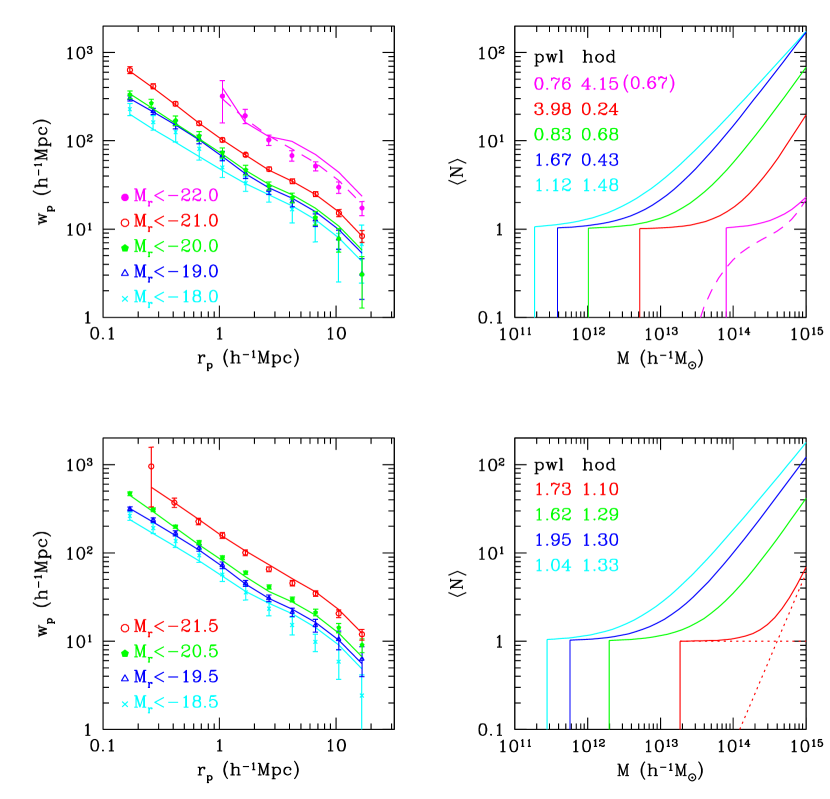
Figure 16: Luminosity dependence of the HOD. Left panels show the measured $w_{p}(r_{p})$ and the best HOD fit for each luminosity-threshold sample. Right panels show the corresponding $\langle N\rangle_{M}$ curves (which shift to the right as the luminosity threshold increases). Also labeled are values of reduced $\chi^{2}$ for the best power-law fit and HOD fit (ordered from top to bottom by decreasing luminosity threshold). The separation of central and satellite galaxies is illustrated for the right-most $\langle N\rangle_{M}$ curve in the lower-right panel (dotted lines). For the brightest sample ($M_{r}<-22$), we show the effect of adding an exponential cutoff profile in $\langle N\rangle_{M}$ (dashed curve in the upper-right panel), which leads to an improved HOD fit (dashed curve in the upper-left panel).

Table 3: Best-fit HOD Parameters for Luminosity-Threshold Samples

${M_{r}}^{\mathrm{max}}$	$\log_{10}M_{\rm min}$	$\log_{10}M_{1}$	$\alpha$	N	$\chi^{2}_{HOD}$	$\chi^{2}_{power-law}$
-22.0	13.91	14.92	1.43	7	20.74 (3.33)	3.81
-21.5	13.27	14.60	1.94	10	8.81	13.81
-21.0	12.72	14.09	1.39	11	2.18	35.78
-20.5	12.30	13.67	1.21	11	11.65	14.57
-20.0	12.01	13.42	1.16	11	6.09	7.48
-19.5	11.76	13.15	1.13	11	11.70	17.53
-19.0	11.59	12.94	1.08	11	3.87	15.06
-18.5	11.44	12.77	1.01	11	11.94	9.38
-18.0	11.27	12.57	0.92	11	13.33	10.04

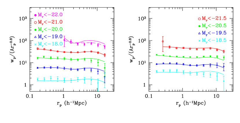
Figure 17: Same as left panels of Fig. 16, but each of the measured and best-fit projected correlation functions is divided by a power-law $\propto r_{p}^{-0.8}$. An arbitrary vertical displacement is applied for each sample. This plot allows a close inspection of departures from a power-law in $w_{p}$.

Figure 18 plots the derived HOD parameters as a function of the threshold luminosity. The characteristic minimum mass $M_{\rm min}$ of halos that can host a galaxy increases as we go to high luminosity samples. For low luminosity samples ($L_{\rm thres}<L^{*}$, with $M_{r}^{*}\sim-20.5$), the minimum host halo mass $M_{\rm min}$ is approximately proportional to the threshold luminosity. Halos near $M_{\rm min}$ generally contain a single, central galaxy above the luminosity threshold, and this linear relation suggests that the stellar light of this central galaxy is approximately proportional to the halo mass in this low luminosity regime. However, as we move to high luminosity galaxies ($L_{\rm thres}>L^{*}$), the minimum mass of hosting halos increases more steeply than a naive linear relation $M_{\rm min}\propto L$. This departure is consistent with the well established fact that these luminous galaxies are found only in group or cluster environments (see e.g., Loh 2003; Blanton et al. 2005a). In these high mass halos, a larger fraction of baryon mass goes into satellites below the luminosity threshold and into a shock-heated intragroup medium, leaving less for the central galaxies. The steepening of the relation between $M_{\rm min}$ and the threshold luminosity toward high luminosity is in good agreement with galaxy formation models (see, e.g., Zheng et al. 2004). Dynamical mass estimates of galaxies from velocity dispersions of stars (e.g., Padmanabhan et al. 2004) or satellite galaxies (e.g., Prada et al. 2003; McKay et al. 2002) and aperture mass measured from weak lensing (e.g., McKay et al. 2001; Sheldon et al. 2004; Tasitsiomi et al. 2004) do not show as strong a dependence on galaxy luminosity, even after correcting to the halo virial mass. However, these results do not necessarily conflict with ours, since $M_{\rm min}$ represents the characteristic minimum mass, not average mass, for galaxies above a given luminosity. Scatter in the relation between galaxy luminosity and host halo mass can substantially weaken the dependence of the average halo mass on galaxy luminosity, as shown by Tasitsiomi et al. (2004).

Figure 18: HOD parameters as a function of the threshold luminosity. The left panel shows $M_{\rm min}$ (solid circles) and $M_{1}$ (empty circles). The dashed curve is the $M_{\rm min}$–$M_{r}$ (solid) curve scaled up by a factor of 23. The two dotted lines plot $M\propto L$ for comparison. The right panel shows the power-law slope $\alpha$ of $\langle N_{\rm sat}\rangle_{M}$. Adopting an exponential cutoff profile in $\langle N\rangle_{M}$ only has a small effect on the inferred $\alpha$ (empty circles versus solid circles).

Figure 18a also shows a small departure from the linear relation at the low luminosity end — relatively larger halos are needed to host faint galaxies. This departure could be a hint of feedback processes suppressing the masses of galaxies in these low mass halos, but this subtle deviation from linearity is sensitive to our idealized assumption of a sharp $M_{\rm min}$ threshold for central galaxies, so with ${w_{p}(r_{p})}$ data alone we cannot address this point reliably.

Open circles in Figure 18a show the mass scale $M_{1}$ of halos that on average host one satellite galaxy above the luminosity threshold (in addition to the central galaxy). For the samples analyzed here, the derived $M_{1}$ and $M_{\rm min}$ have an almost perfect scaling relation: $M_{1}\approx 23M_{\rm min}$ (dashed line). This striking result tells us that a halo hosting two galaxies above a luminosity threshold must be, on average, at least 20 times as massive as a halo hosting only one galaxy above the threshold. This result is consistent with the slowly rising plateau of $\langle N\rangle_{M}$ found for SPH and semi-analytic model galaxies by Berlind et al. (2003) and for $N$-body subhalos by Kravtsov et al. (2004). Berlind et al. (2003) show that in the regime where $1\leq\langle N\rangle_{M}\leq 2$, higher mass halos tend to host higher mass central galaxies rather than multiple galaxies of comparable mass. The exact scaling factor depends on our assumption of the spatial distribution of galaxies inside halos. If we reduce the concentration parameter of the galaxy distribution at each halo mass by a factor of two, we can still get reasonable fits to the data, but $M_{1}$ and $\alpha$ decrease to allow more galaxies in low mass, high concentration halos, and the scaling factor drops to $M_{1}/M_{\rm min}\approx 17$. If we increase the concentrations by a factor of two, then the linear scaling relation becomes less accurate, and the factor is $M_{1}/M_{\rm min}\approx 30$. The roughly constant factor of $\sim 20$ at all luminosities agrees qualitatively with predictions from $N$-body simulations, SPH simulations, and semi-analytic models (see Kravtsov et al. 2004; Zheng et al. 2004), but establishing quantitative agreement over this large dynamic range in luminosity remains a challenge for further theoretical studies of galaxy formation. The large value of this factor probably reflects the combination of halo merger statistics and dynamical friction timescales; near-equal mass mergers of halos are relatively rare, and they are followed fairly quickly by mergers of their central galaxies.

The power-law slope $\alpha$ of the satellite mean occupation number $\langle N_{\rm sat}\rangle_{M}$ rises slowly but steadily ($\alpha\simeq 0.9$ to $\alpha\simeq 1.2$) with luminosity for thresholds $L_{\rm thres}<L^{*}$, then rises more steeply for higher luminosity thresholds (Figure 18b). A straightforward interpretation of this trend would be that halos of higher mass have greater relative efficiency at producing multiple high luminosity satellites. Studies on substructures in high resolution numerical simulations indicate that more massive halos tend to have relatively more substructures of higher masses (see, e.g., Figures 5 and 7 of Gao et al. 2004 and Figure 1 of De Lucia et al. 2004), consistent with the trend we find in $\alpha$. However, while the statistical errorbars on $\alpha$ (as indicated in the figure) are small, systematic errors in $\langle N\rangle_{M}$ resulting from our restricted parameterization of the HOD could be more important. Kravtsov et al. (2004) typically find that $\alpha=1.00\pm 0.05$ for samples of $N$-body subhalos selected based on maximum circular velocities, while their Figures 4–6 show that $\langle N_{\rm sat}\rangle_{M}$ drops faster than a power-law at the low mass end. Motivated by this result, we tried changing our parameterization of the satellite mean occupation from $\langle N_{\rm sat}\rangle_{M}=(M/M_{1})^{\alpha}$ to $\langle N_{\rm sat}\rangle_{M}=\exp[-M_{\rm cut,sat}/(M-M_{\rm min})](M/M_{1}^{\prime})$, with the same truncation at $M=M_{\rm min}$. This formulation has the same number of free parameters, but it fixes $\alpha=1$ and changes the sharp cutoff at $M=M_{\rm min}$ to an adjustable exponential cutoff. Although the number of satellites is small in the exponential cutoff region, the freedom afforded by $M_{\rm cut,sat}$ breaks the connection between the value of $\alpha$ and the normalization of $\langle N_{\rm sat}\rangle_{M}$, so it has a significant impact on $w_{p}(r_{p})$; making $\alpha>1$ or suppressing satellite numbers at low halo mass both increase the one-halo contribution from higher mass halos.

We find that this parameterization yields $w_{p}(r_{p})$ fits close to those of our sharp cutoff, variable $\alpha$ parameterization, as shown for the $M_{r}<-21$ sample in Figure 19a. However, the relation between $M_{\rm min}$ and the mass scale $M_{\rm 1,sat}$ where $\langle N_{\rm sat}\rangle_{M}=1$ remains very close to our original result of $M_{\rm 1,sat}\sim 23M_{\rm min}$, indicating that this scaling relation is robust. Another quantity that is robust to these changes is the central to satellite galaxy ratio implied from the HOD model. For the $M_{r}<-21$ sample, $85\%$ of galaxies are central galaxies in the halos and only $15\%$ make up the satellite distribution. Central galaxies dominate over satellites for nearly all of our samples, with an interesting exception that we discuss in §4.3 below. Figure 19b shows that the mean occupations for the two parameterizations are in fact very similar for $M<10^{15}h^{-1}M_{\odot}$; we cannot distinguish between the parameterizations because more massive halos are too rare to contribute significantly to ${w_{p}(r_{p})}$. Other complementary statistics, most notably the group multiplicity function, are sensitive to $\langle N\rangle_{M}$ at high $M$. In the long run, we can use the multiplicity function to pin down the high-$M$ regime and add greater flexibility to our parameterization of $\langle N\rangle_{M}$ in the regime of the low mass cutoff and the plateau where $\langle N\rangle_{M}$ rises from one to several. To illustrate the level of uncertainty in $\langle N\rangle_{M}$ with ${w_{p}(r_{p})}$ alone, Figure 19c shows fits using a much more flexible HOD parameterization (Z. Zheng & D. Weinberg 2005, in preparation) that allows a smooth cutoff in $\langle N_{\rm cen}\rangle_{M}$ and describes $\langle N_{\rm sat}\rangle_{M}$ by a cubic spline connecting five values specified at intervals in $\log_{10}M$, a total of seven free parameters of which one is fixed by the mean galaxy density. The ten models shown all have $\Delta\chi^{2}\leq 1$ with respect to the best-fit of the flexible HOD parameterization, which itself has a $\chi^{2}$ that is 1.38 lower than that of our best-fit two-parameter model. The central to satellite ratio is again quite robust to these changes, with a corresponding $1\sigma$ range of $14.5\%-16.5\%$ for the satellite fraction.

Figure 19: Fits to ${w_{p}(r_{p})}$ of the $M_{r}<-21$ sample with different HOD parameterizations. The left panel shows the measured and predicted values of $w_{p}(r_{p})$ (with two curves nearly superposed), and the middle panel shows the corresponding $\langle N\rangle_{M}$. Dashed curves are results of using our standard HOD parameterization ($\alpha$ is a free parameter), and solid curves are from a parameterization that fixes $\alpha=1$ and adjusts the cutoff mass of $\langle N_{\rm sat}\rangle_{M}$. In the middle panel, the thin and thick dotted curves are mean occupation numbers of satellite galaxies for the former and latter case, respectively. Fits from these two forms of HOD are very close to each other. The right-hand panel shows $\langle N\rangle_{M}$ fits when using a more flexible HOD parametrization (see text). Ten different models are shown, all with $\Delta\chi^{2}<1$ relative to the best-fit model. The solid lines correspond to $\langle N\rangle_{M}$ and the dashed lines show $\langle N_{\rm sat}\rangle_{M}$.

Returning to our standard parameterization, Figure 16 shows that no choice of parameters yields a good fit for the brightest sample ($M_{r}<-22$) — the predicted $w_{p}(r_{p})$ for the best fit model is $\sim$50% too high at large $r_{p}$. Our HOD modeling is applied at $z\sim 0$ and does not incorporate evolution of the growth factor, while this bright sample extends to $z\sim 0.22$, where $\sigma_{8}$ is lower by $\sim$10%. However, we find that the fit does not improve substantially if we lower $\sigma_{8}$ to the value at the sample’s median redshift, $z_{\rm med}\sim 0.17$. The masses of halos hosting these very luminous galaxies are above $\sim 10^{14}h^{-1}M_{\odot}$, and in this regime the analytic formula of Sheth, Mo, & Tormen (2001) that we adopt for the halo bias factor may over-predict the halo bias (see their Figure 6). A 10% over-prediction of the halo bias factor would boost the large-scale correlation function by about 20%. If we adopt the Seljak & Warren (2004) bias factors and keep our standard treatment of halo exclusion and scale dependence of halo bias, then we obtain a reasonably good fit to ${w_{p}(r_{p})}$ for this sample, though we now underpredict ${w_{p}(r_{p})}$ for some fainter samples.

Another potential explanation for this discrepancy, and the most physically interesting one, is that our assumption of a sharp threshold at $M_{\rm min}$ is too idealized for this high luminosity sample. In general, the map from halo mass to central galaxy luminosity is not one-to-one, so the transition from no central galaxy to one central galaxy in luminosity-threshold galaxy samples should occur over some range of mass. To illustrate the effect, we apply an exponential cutoff profile $\exp(-M_{\rm min}/M)$ to both $\langle N_{\rm cen}\rangle_{M}$ and $\langle N_{\rm sat}\rangle_{M}$. (The model shown previously in Figure 19b applied a smooth cutoff only to satellite galaxies.) This parameterization leads to a much better fit (dashed curve in the upper-left panel of Figure 16), while the number of free parameters remains the same (still $M_{1}$ and $\alpha$, with $M_{\rm min}$ fixed by the number density constraint). A soft cutoff profile reduces the large-scale galaxy bias factor by allowing some galaxies in the sample to populate lower mass halos with lower bias factors. We find that changing the HOD in this way yields slightly better fits for most other samples but that the derived parameters ($M_{\rm min}$, $M_{1}$, and $\alpha$) are not very different from the sharp threshold case, as demonstrated for $\alpha$ in Figure 18b (dotted line). Allowing a smooth cutoff in $\langle N_{\rm cen}\rangle_{M}$ has a much larger impact on the $M_{r}<-22$ sample than on the lower luminosity samples because the halo bias factor and halo space density change rapidly with mass for high mass halos. Tasitsiomi et al. (2004) also find that, in their $N$-body model, a scatter in the luminosity-maximum velocity (mass) relation helps to reduce the predicted galaxy-mass correlation function of bright galaxies ($-22.2\leq M_{r}\leq-21.7$) and thus reproduce that measured by Sheldon et al. (2004). Definitive numerical results for the halo bias factor at high masses would allow stronger conclusions on this interesting point, since Figure 16 shows that the large scale amplitude of ${w_{p}(r_{p})}$ for bright samples should have an easily measurable dependence on this scatter.

So far, we have concentrated on luminosity-threshold samples, for which the HOD can be parameterized in a simple way. Our step-function plus power-law parameterization is not appropriate for a luminosity-bin sample, since high mass halos have central galaxies that fall out of the bin because they are too bright. However, we can infer the HOD for a sample of galaxies in a luminosity bin $L_{\rm thres,1}<L<L_{\rm thres,2}$ from the difference in the fitted HOD models for the two luminosity-threshold samples $L>L_{\rm thres,1}$ and $L>L_{\rm thres,2}$. The separation of central and satellite galaxies in our parameterization simplifies this translation. For a luminosity-bin sample, the mean occupation number of central galaxies is just the difference between two step functions, which becomes a square window, while that of satellite galaxies is the difference of two power law functions. We use the parameterization with $\alpha=1$ and $\langle N_{\rm sat}\rangle_{M}=\exp[-M_{\rm cut,sat}/(M-M_{\rm min})](M/M_{1}^{\prime})$ (see Fig. 19), so that small differences in $\alpha$ do not produce anomalous behavior in the difference of occupation functions at high $M$.

Figure 20b shows the mean occupation functions for three luminosity bins derived in this way from our luminosity-threshold results. The majority of galaxies in each luminosity bin are central galaxies, with their relative fraction increasing with luminosity (about 55%, 65%, and 75%, respectively, and 85% for the $-22<M_{r}<-21$ case not shown in the plot). Our restricted HOD parameterization might lead to an underestimate of the fraction of central galaxies for low luminosity samples; with the more flexible cubic spline parameterization mentioned above we find that the 1-$\sigma$ range of the central galaxy fraction is 69%–78% for the $-20<M_{r}<-19$ sample and 75%–81% for the $-21<M_{r}<-20$ sample, compared to 65% and 75% for the best-fit two-parameter model. Nevertheless, the general trend of increased central galaxy fraction with luminosity remains the same. Figure 20a compares the predicted $w_{p}(r_{p})$ curves with the measured data points for each bin. While the threshold and bin correlation functions are obviously not independent, it is nonetheless encouraging that predictions derived from the threshold samples match measurements for bin samples fairly well, suggesting that our adopted parameterization for luminosity-threshold samples is reasonable. Our differencing of luminosity-threshold HODs yields a luminosity-bin HOD parameterization similar to that adopted by Guzik & Seljak (2002) in their models of SDSS galaxy-galaxy lensing.

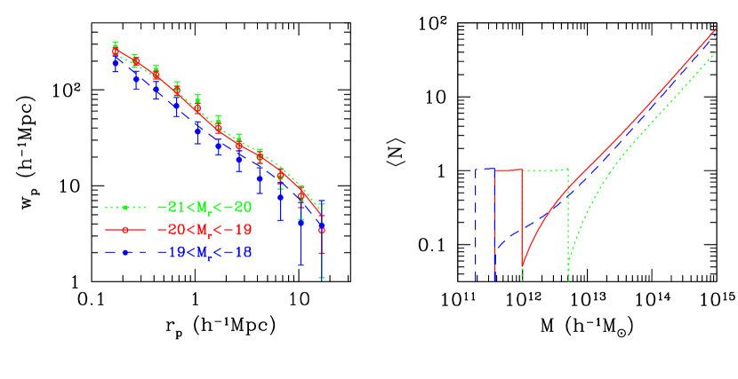
Figure 20: Predictions of ${w_{p}(r_{p})}$ and HODs for luminosity-bin samples based on HOD parameters inferred from luminosity-threshold samples. The left panel compares measured (points) and predicted (curves) ${w_{p}(r_{p})}$ for three luminosity-bin samples. Right panels show the $\langle N\rangle_{M}$ curves used for the predictions, each of which is the difference of two luminosity-threshold $\langle N\rangle_{M}$ curves.

Knowing the mean occupation function of galaxies in each luminosity bin, we can also easily predict the conditional luminosity function (CLF; Yang, Mo, & van den Bosch 2003), defined as the average number of galaxies per unit luminosity that reside in a halo of given mass. Through fitting luminosity functions and luminosity-dependent clustering simultaneously, the CLF offers an alternative approach to HOD modeling, and it has been used to model observations from the 2dFGRS and the DEEP2 redshift survey and to construct mock galaxy catalogs (Yang, Mo, & van den Bosch 2003; van den Bosch, Yang, & Mo 2003a; van den Bosch, Mo, & Yang 2003b; Mo et al. 2004; Yan, Madgwick, & White 2003; Yan, White & Coil 2004). These papers have parameterized the CLF as a Schechter (1976) function with normalization, faint end slope, and characteristic luminosity depending on halo mass. Here, we take a different approach to the CLF — instead of assuming an a priori functional form, we ask what the measured luminosity dependence of galaxy clustering can tell us about the shape of the CLF. The information for inferring the CLF at each halo mass is fully encoded in the best fit HOD parameters of different luminosity-threshold samples, and at a given halo mass $M$ one only needs to take differences of $\langle N\rangle_{M}$ for adjacent luminosity thresholds: $\Phi(L_{1}<L<L_{2}|M)\propto\langle N(>L_{1})\rangle_{M}-\langle N(>L_{2})\rangle_{M}.$ Figure 21 shows the inferred CLF at three halo masses for two forms of the HOD parameterization, a step-like cutoff in $\langle N\rangle_{M}$ in left-hand panels and an exponential cutoff in right-hand panels. Central galaxies produce a marked departure from a Schechter-like form, especially in low mass halos where they contain a larger fraction of the total luminosity. The prominence of the central galaxy peak is much stronger for a step-function parameterization than for an exponential cutoff form, but it is present in either case. An accurate empirical determination of the CLF via this route would require more complementary clustering measurements so that the low mass cutoff of $\langle N_{\rm cen}\rangle_{M}$ and $\langle N_{\rm sat}\rangle_{M}$ can be well constrained. Semi-analytic galaxy formation models and SPH simulations suggest that the CLF can be modeled as the sum of a truncated Schechter function representing satellite galaxies and a Gaussian function representing central galaxies (Zheng et al. 2004), qualitatively consistent with the results in Figure 21.

Figure 21: Conditional luminosity functions of galaxies inferred from the best-fit HOD parameters for the luminosity threshold samples, shown at three different halo mass scales. Results from two variants of the HOD parameterizations are shown: a step-like cutoff in $\langle N\rangle_{M}$ (left-hand panels) and an exponential cutoff profile (right-hand panels). Dashed lines show the contribution from central galaxies and dotted lines the contribution from satellites. In the step-like cutoff cases, the central galaxies contribute only to the highest magnitude bin. The CLF in each panel is arbitrarily normalized such that the total number of galaxies in each halo is one.

4.3 Modeling the Color Dependence

As we saw in § 3.3, red galaxies are more strongly clustered than blue galaxies. A qualitative explanation is that red galaxies preferentially reside in galaxy groups and clusters. Within the HOD framework, we can understand the color dependence in a quantitative way by inferring the relative distribution of blue and red galaxies as a function of halo mass from the clustering data. We model the same sequence of luminosity bins shown in Figure 14, except that our brightest sample consists of all galaxies with $M_{r}<-21$ instead of the $-22<M_{r}<-21$ magnitude bin. We again use the luminosity-dependent color cut of Figure 12 to define red and blue subsamples, so that red galaxies correspond roughly to the distinctive red sequence. Red galaxies predominate in the most luminous sample, and blue galaxies predominate in the two faintest samples. Table 4 lists the number of galaxies and number densities in each sample.

For each luminosity sample, we simultaneously fit the the projected correlation functions of red, blue, and all (red+blue) galaxies to infer their HOD parameters. We can obtain the mean occupation functions for blue and red galaxies from that of all galaxies by modeling the blue galaxy fraction, $f_{b}$, as a function of halo mass. Since our parameterization distinguishes central and satellite galaxies, and the blue fractions for these two populations could well be different, we separately parameterize $f_{b}$ for central galaxies and for satellites. We know that red galaxies are more common in high mass halos, so we adopt functional forms in which $f_{b}$ is a decreasing function of halo mass, such as a log-exponential,

$$f_{b}(M)=f_{0}\exp\left(-\frac{\log_{10}M-\log_{10}M_{\rm min}}{\sigma_{M}}\right),$$ (10)

or a log-normal

$$f_{b}(M)=f_{0}\exp\left[-\frac{(\log_{10}M-\log_{10}M_{\rm min})^{2}}{2\sigma_{M}^{2}}\right].$$ (11)

We find that these two functions fit the data equally well. Motivated roughly by theoretical predictions (Zheng et al. 2004), we adopt the log-normal form for the blue fraction $f_{b,{\rm cen}}$ in central galaxies and the log-exponential form for the blue fraction $f_{b,{\rm sat}}$ in satellite galaxies. There are two parameters in each function: $f_{0}$, the blue fraction in halos of $M=M_{\rm min}$, and $\sigma_{M}$, a quantity characterizing how fast the blue fraction drops. Of the four new parameters, one (e.g., $f_{0,{\rm cen}}$) can be fixed by matching the global number density of blue galaxies. We assume that red and blue satellite galaxies follow Poisson distributions with respect to their mean occupations $\langle N_{r,{\rm sat}}\rangle_{M}$ and $\langle N_{b,{\rm sat}}\rangle_{M}$, just as in the full satellite sample. It is well known that there is color/morphology segregation within galaxy clusters (e.g., Oemler 1974; Melnick & Sargent 1977; Dressler 1980; Adami, Biviano, & Mazure 1998) — red galaxies are more centrally concentrated. With the $w_{p}(r_{p})$ data alone, we have little power to constrain the relative concentration of red and blue galaxies, since the effect shows up only on small scales and can be compensated by changing the relative satellite occupation numbers. We therefore do not consider the segregation effect here. We find that we can obtain good fits by assuming that both satellite populations follow the same NFW profile as the dark matter. Constraints on the profiles of red and blue satellites could be better obtained from direct analysis of identified groups, after which these profiles could be imposed in $w_{p}(r_{p})$ fitting. Altogether, then, we have five free parameters ($M_{1}$, $\alpha$, $f_{0,{\rm sat}}$, $\sigma_{M,{\rm cen}}$, and $\sigma_{M,{\rm sat}}$) to simultaneously fit the projected correlation functions of red, blue, and all galaxies, with the parameters $M_{\rm min}$ and $f_{0,{\rm cen}}$ fixed by number density constraints.

Figure 22 shows fitting results for the luminous ($M_{r}<-21$) sample. The best-fitting HOD parameters are listed in Table 4. With the five-parameter model, we obtain an excellent fit to 32 data points, with $\chi^{2}/{\rm d.o.f.}=0.62$ (upper-left panel), showing that the different spatial clustering of red and blue galaxies can be well explained by their different occupations of dark matter halos. In the fits, the mean occupation number of red galaxies rises continuously with halo mass, while $\langle N\rangle_{M}$ for blue galaxies shows a minimum near $3\times 10^{13}h^{-1}M_{\odot}$. As halo mass increases, the total blue fraction (lower-left panel) has a sharp drop, a small rise, then a gentle decline. The non-monotonic behavior is easily understood when we separate the contributions of central and satellite galaxies. In halos just above $M_{\rm min}$, central galaxies are predominantly blue, but above $\sim 2M_{\rm min}$ they are predominantly red. The minimum in the blue galaxy occupation occurs for halos that are too massive to have a blue central galaxy but not massive enough to have any satellite galaxies above our luminosity threshold. This transition explains why the mean occupation number of blue galaxies can be approximated by a Gaussian bump (or a square window) plus a power-law, as used in some HOD models (e.g., Sheth & Diaferio 2001; Scranton 2003); the two components represent blue central and satellite galaxies, respectively (see Guzik & Seljak 2002). The blue satellite fraction declines slowly with halo mass in the regime $M\gtrsim 20M_{\rm min}$ where satellite galaxies are common.

Table 4: Volume-limited Correlation Function Red/Blue Samples and Best-fit HOD Parameters

$M_{r}$	$N_{\mathrm{gal,red}}$	$N_{\mathrm{gal,blue}}$	${\bar{n}}_{\mathrm{red}}$	${\bar{n}}_{\mathrm{blue}}$	$\log_{10}M_{\rm min}$	$\log_{10}M_{1}$	$\alpha$	$f_{\mathrm{0,cen}}$	$f_{\mathrm{0,sat}}$	$\sigma_{M,{\rm cen}}$	$\sigma_{M,{\rm sat}}$	$\frac{\chi^{2}}{d.o.f.}$
$<$ -21	16,142	9,873	0.0726	0.0444	12.72	14.08	1.37	0.71	0.88	0.30	1.70	0.62
-21 $-$ -20	2,881	2,789	0.245	0.237	12.00	13.38	1.16	0.55	0.31	10.0	20.0	0.88
-20 $-$ -19	5,804	8,419	0.347	0.503	11.62	12.94	1.06	0.71	0.46	10.0	7.99	0.72
-19 $-$ -18	1,195	3,350	0.267	0.747	11.38	12.58	0.95	0.86	4.00	10.0	0.69	1.48

Note. — The $M_{r}<-21$ sample use $14.5<r\lesssim 17.77$ and others use $10.0<r\lesssim 17.5$. The mean number density (${\bar{n}}_{\mathrm{red}}$ or ${\bar{n}}_{\mathrm{blue}}$) is measured in units of $10^{-2}$ $h^{3}$ Mpc^-3. Mass is in unit of $h^{-1}M_{\odot}$.

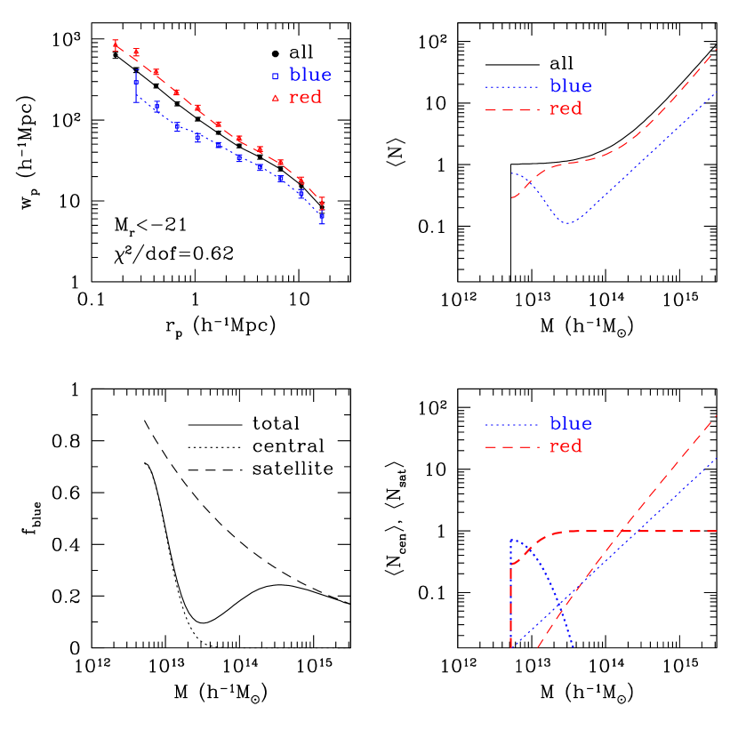
Figure 22: Color dependence of the HOD for the $M_{r}<-21$ sample. The upper-left panel shows measurements of ${w_{p}(r_{p})}$ and best HOD fits for red, blue, and all galaxies in the sample. Mean occupation numbers of these three classes of galaxies are plotted in the upper-right panel. The lower-right panel shows mean occupation numbers of central (thick curves) and satellite (thin curves) galaxies for red (dashed) and blue (dotted) galaxies. The lower-left panel plots the blue fraction for all galaxies (solid curve), central galaxies (dotted curve), and satellite galaxies (dashed curve).

Our detailed numbers for red and blue galaxy HODs should not be taken too seriously because they depend to some degree on our particular choice of parameterized model. This model provides a good fit to the data, but we do not claim that the fit is unique. Nonetheless, when we initially investigated the color dependence using a quite different parameterization that did not distinguish central and satellite galaxies (but accounted for sub-Poisson fluctuations at low halo masses), we were driven to a similar non-monotonic behavior of the blue galaxy $\langle N\rangle_{M}$. Furthermore, our results agree qualitatively with the behavior predicted by SPH simulations and semi-analytic models of galaxy formation. This can be seen by comparing our Figure 22 to Figure 13 of Berlind et al. (2003), which divides the theoretical galaxy population based on mean stellar age (which should correlate strongly with color). Zheng et al. (2004) further analyze these predictions in terms of central and satellite galaxies, again showing good qualitative agreement with our results (compare our Figure 22 to their Figure 4). Semi-analytic and SPH calculations both predict that a halo’s central galaxy is in general more massive and older than its satellites and that the ages of both central and satellite galaxies correlate with halo mass (Berlind et al. 2003, Figures 18 and 19). Physically, these trends reflect the earlier formation times and more active merger histories of central galaxies. Satellite galaxies have generally experienced most of their growth in lower mass halos that merged into their present day parent halos. These physical processes thus lead rather naturally to a trend in which low mass halos have blue central galaxies, higher mass halos have red central galaxies but a significant blue fraction in their satellite populations, and the highest mass halos have red central galaxies and predominantly red satellites. Figure 22 shows the impact of these processes on the galaxy correlation function.

For galaxies of lower luminosities, we study the color division using luminosity-bin rather than luminosity-threshold samples, since the galaxy color distribution depends strongly on luminosity, and we want to isolate the color dependence of the HOD from luminosity dependence. Following our earlier procedure for luminosity-bin samples, we form the mean occupation function for galaxies with $L_{\rm thres,1}<L<L_{\rm thres,2}$ from the difference between two luminosity-threshold samples, $L>L_{\rm thres,1}$ and $L>L_{\rm thres,2}$, then predict $w_{p}(r_{p})$. We determine HOD parameters for the full $L>L_{\rm thres,2}$ sample by fitting $w_{p}(r_{p})$ of that sample, and we parameterize blue fractions as for the $M_{r}<-21$ sample discussed above, so that we still have five free parameters in total to fit projected correlation functions for red, blue, and all galaxies. This approach of working our way down bin by bin is not statistically optimal, since we do not fit all the data simultaneously, and errors in the HOD fit at high luminosities will propagate into lower luminosity bins. However, this procedure is straightforward, and it is adequate for our rather qualitative purposes here, where we seek to understand general features of the HOD color dependence.

Figure 23 shows the results of these fits for the three luminosity bin samples. The HOD parameters for all the samples are specified in Table 4. For $-21<M_{r}<-20$ (with $z_{\rm max}=0.06)$, the fit is formally acceptable ($\chi^{2}/{\rm d.o.f.}=0.88$), but the predicted correlations at large scales are systematically too high, by $\sim 0.5-1\sigma$. For $-20<M_{r}<-19$, the fit is excellent for all, red, and blue galaxies, with the HOD model nicely explaining the strong inflection of the red galaxy ${w_{p}(r_{p})}$ near $2\,h^{-1}\;{\rm Mpc}$. For $-19<M_{r}<-18$, the fit overpredicts the correlation of galaxies on large scales, but the small volume of this faintest sample leaves it somewhat susceptible to cosmic variance. In every case our fits capture the qualitative difference between red and blue galaxy clustering, and we do not know whether the quantitative discrepancies reflect underestimates of observational errorbars or inadequacy of this simple, five-parameter model.

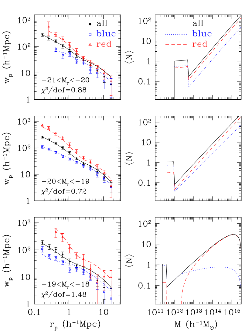
Figure 23: Color dependence of the HOD for the three luminosity-bin samples. For each luminosity bin, the left panel shows the ${w_{p}(r_{p})}$ measurements and best HOD fits for red, blue and all galaxies. The right panel shows the corresponding $\langle N\rangle_{M}$ for these three classes of galaxies.

If we take the fit results at face value, we see that as luminosity decreases the central galaxies occupy lower and lower mass halos (as already seen in Figs. 16 and 20) and become more and more dominated by blue galaxies (56%, 71%, and 85%, respectively). For all three luminosity bins, the majority ($\sim 70-90\%$) of blue galaxies are central objects. The majority of red galaxies are also central in the brightest bins, but the fraction of red galaxies that are satellites becomes larger with decreasing luminosity (35%, 54%, and 72% for the three samples). Thus, faint red galaxies are predominantly satellite systems in higher mass halos. To put the result in physical terms, low mass galaxies have late star formation and blue colors if they reside in “the field” (making them central objects of low mass halos) and become red only if they enter dense environments that truncate their star formation, a behavior predicted in SPH simulations (Berlind et al., 2005). Again, our detailed numbers should be taken with a grain of salt because of the restrictions of the parameterization, but the fitting results show a sensible continuity of behavior as we move from luminous galaxies to faint galaxies.

Since faint and bright red galaxies both reside in high mass halos, as satellites and central objects, respectively, the average host halo mass of red galaxies is actually lowest for intermediate luminosities. From our fits, we find a mean host halo mass $\sim 2-2.5\times 10^{14}h^{-1}M_{\odot}$ for red galaxies with $-18>M_{r}>-19$ and $M_{r}<-22$, compared to $\sim 10^{14}h^{-1}M_{\odot}$ for $-19>M_{r}>-22$. This non-monotonic behavior explains why faint and bright red galaxies have higher correlation amplitudes (Fig. 14 here and Norberg et al. 2002) and denser local environments (Hogg et al., 2003) than intermediate luminosity red galaxies.

Dividing into blue and red subsamples allows another useful measurement, the cross correlation between blue and red galaxies. At large scales, where the two-halo term dominates, there is little new information in the cross correlation because it is essentially guaranteed to approach the geometric mean of the red and blue galaxy autocorrelations. However, in the one-halo regime the cross correlation encodes information about the halo-by-halo mixing of the red and blue populations. At one extreme, we could imagine that some halos contain only red galaxies and others only blue galaxies, and the ratio of the mean occupations represents the ratio of “red halos” to “blue halos”. In this case, the one-halo term of the cross-correlation function would be zero. At the other extreme, the red and blue populations are fully mixed, and the typical red-to-blue ratio in each halo is just the ratio of mean occupations. In this case, the one-halo contribution to the cross-correlation reaches its maximum amplitude. Our modeling of the autocorrelation functions has implicitly assumed this fully mixed case, since we have taken the numbers of red and blue satellites within each halo to be Poisson distributed with respect to their mean occupations. The cross-correlation measurement allows an independent test of this assumption.

The one-halo term of the real space cross-correlation function of red and blue galaxies can be computed as

$$1+\xi_{\rm rb,1h}(r)=\frac{1}{4\pi r^{2}\bar{n}_{r}\bar{n}_{b}}\int_{0}^{\infty}dM\frac{dn}{dM}\langle N_{r}N_{b}\rangle_{M}\frac{1}{2R_{\rm vir}(M)}F^{\prime}\left(\frac{r}{2R_{\rm vir}};c_{r},c_{b}\right),$$ (12)

where $\bar{n}_{r}$ and $\bar{n}_{b}$ are the mean number densities of red and blue galaxies, respectively, $\langle N_{r}N_{b}\rangle_{M}$ is the average number of red-blue galaxy pairs in a halo of mass $M$, $F(r/2R_{\rm vir};c_{r},c_{b})$ is the cumulative radial distribution of red-blue galaxy pairs, and $c_{r}$ and $c_{b}$ are the concentration parameters of red and blue galaxies ($c_{r}=c_{b}$ is assumed in this paper). This equation is similar to equation (8). With the separation of central and satellite galaxies, the pair distribution can be expressed as in equation (9):

$$\langle N_{r}N_{b}\rangle_{M}F^{\prime}(x;c_{r},c_{b})=\newline \langle N_{r,{\rm cen}}N_{b,{\rm sat}}\rangle_{M}F^{\prime}_{\rm cs}(x;c_{b})+\langle N_{r,{\rm sat}}N_{b,{\rm cen}}\rangle_{M}F^{\prime}_{\rm cs}(x;c_{r})+\langle N_{r,{\rm sat}}N_{b,{\rm sat}}\rangle_{M}F^{\prime}_{\rm ss}(x;c_{r},c_{b}),$$ (13)

where $F^{\prime}_{\rm cs}$ has the same meaning as in equation (9) and $F^{\prime}_{\rm ss}$ now represents the cross-convolution of two NFW profiles. If red and blue galaxies are well mixed and their occupation numbers are not correlated, then the average number of any kind of blue-red galaxy pairs on the right-hand side of equation (13) can be replaced by the product of the mean occupation numbers of blue and red galaxies, e.g., $\langle N_{r,{\rm cen}}N_{b,{\rm sat}}\rangle_{M}=\langle N_{r,{\rm cen}}\rangle_{M}\langle N_{b,{\rm sat}}\rangle_{M}$. The extreme example of “red halos” and “blue halos,” on the other hand, corresponds to $\langle N_{r,{\rm cen}}N_{b,{\rm sat}}\rangle_{M}=\langle N_{r,{\rm sat}}N_{b,{\rm cen}}\rangle_{M}=\langle N_{r,{\rm sat}}N_{b,{\rm sat}}\rangle_{M}=0$.

We estimate the cross-correlation function from the data in an analogous way to the autocorrelations, using equation (1) with $DD$ replaced by $D_{1}D_{2}$, $2DR$ by $D_{1}R_{2}+D_{2}R_{1}$, and $RR$ by $R_{1}R_{2}$, with the subscripts denoting the two subsamples. In Figure 24, we compare the projected cross-correlation function for the $M_{r}<-21$ sample (filled circles) to the prediction assuming the fully mixed case (solid line). The other points and lines in the figure show the measured and predicted autocorrelations (from Figure 22) and their geometric means. The predicted cross-correlation is close to the measured one, though it is systematically higher at $r_{p}\lesssim 1h^{-1}{\rm Mpc}$ (the $\chi^{2}$ for the 11 data points is about 15, most of which comes from small scales). At large scales, where the two-halo term dominates, the predicted and measured cross-correlation functions approach the geometric means as expected. For the extreme case of distinct red and blue halos, there would be no one-halo contribution to the cross-correlation function, and the projected cross-correlation would flatten at $r_{p}\lesssim 2h^{-1}{\rm Mpc}$ (see Figure 24). This is clearly not the case in the data. Our simple assumption of well mixed blue and red satellite populations with similar radial profiles appears to describe the one-halo regime of the cross-correlation fairly accurately, though the fit is not perfect, and it is probably not unique. Direct measurement of the distributions of red and blue galaxy numbers in identified groups can test our assumption.

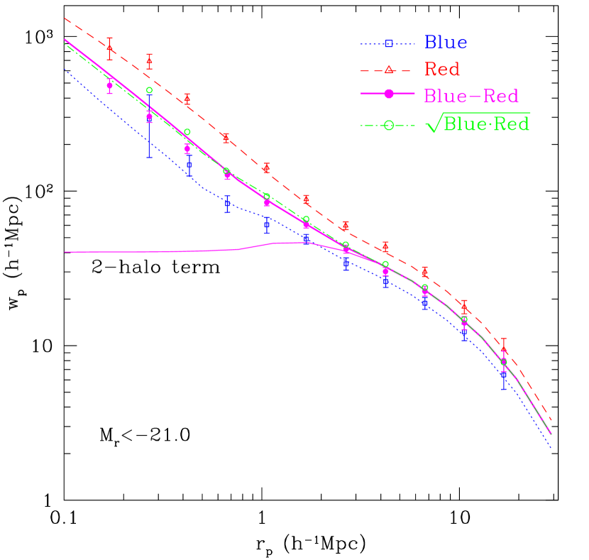
Figure 24: Projected cross-correlation between red and blue galaxies in the $M_{r}<-21$ sample. Points are measurements. Dotted and dashed curves are HOD fits to auto-correlations of blue and red galaxies, respectively. The dot-dashed curve is the geometric mean of the two fits. HOD parameters of these fits are obtained by simultaneously fitting $w_{p}$ of red, blue, and all galaxies, i.e., the same as in Fig. 22. The thick solid curve is the predicted cross-correlation between red and blue galaxies based on these HOD parameters, with the assumption that blue and red galaxies are well mixed within halos. The thin solid curve is the two-halo term of the cross-correlation, representing the case in which blue and red galaxies avoid residing in the same halo (see the text).

5 Conclusions

We have exploited the large size and high quality imaging of the SDSS galaxy redshift survey to study the detailed dependence of the galaxy two-point correlation function on galaxy luminosity and color. The amplitude of the projected correlation function ${w_{p}(r_{p})}$ increases monotonically with luminosity, slowly below $L_{*}$ and rapidly above. The real space correlation functions of luminosity-bin or luminosity-threshold samples are usually described to a first approximation by a power-law $\xi(r)=(r/r_{0})^{-1.8}$, with the exception of the brightest samples ($-23<M_{r}<-22$ luminosity-bin or $M_{r}>-22$ luminosity-threshold), which have a substantially steeper $\xi(r)$. However, an inflection in ${w_{p}(r_{p})}$ at $r_{p}\sim 1-3\,h^{-1}\;{\rm Mpc}$, which is clearly identifiable for $M_{r}<-21$ galaxies (Z04), is also present to some degree in many of our other volume-limited samples, and it is unmistakably present in the high-precision measurement from the full, flux-limited data sample. The projected correlation function of the $b_{J}$-selected, 2dFGRS survey shows a similar feature (Hawkins et al. 2003, Figure 9).

Dividing galaxies by color, we find that red galaxies have stronger clustering, steeper correlation functions at small scales, and much stronger “finger-of-God” redshift-space distortions. The blue galaxies in luminosity-bin samples usually have correlation functions close to an $r^{-1.7}$ power-law, with amplitudes that increase with luminosity. For red galaxies, the situation is more complex. Red galaxy correlation functions are consistently steeper than $r^{-1.8}$, but the relative bias as a function of luminosity is scale-dependent, with bright red galaxies exhibiting the strongest clustering on large scales and faint red galaxies exhibiting the strongest clustering on small scales. The luminosity and color dependence of ${w_{p}(r_{p})}$ are not trivially separable, nor is one a simple consequence of the other.

Our conclusion that clustering increases with luminosity, most markedly above $L_{*}$, agrees with many previous investigations (Hamilton, 1988; Park et al., 1994; Loveday et al., 1995; Benoist et al., 1996; Guzzo et al., 1997). The relative bias $b/b_{*}$ as a function of $L/L_{*}$, defined using the ratio of ${w_{p}(r_{p})}$ values at $r_{p}=2.7\,h^{-1}\;{\rm Mpc}$, agrees with that inferred (from essentially the same galaxy sample) using the large scale power spectrum by Tegmark et al. (2004a). This measurement is also in good agreement with the fit of Norberg et al. (2001) derived from the 2dFGRS, over the (somewhat narrower) luminosity range of their measurements.

Our finding of stronger clustering of “early” type (which in our case means red) galaxies agrees with decades of results obtained by a variety of techniques (e.g., Hubble 1936; Zwicky et al. 1968; Davis & Geller 1976; Dressler 1980; Postman & Geller 1984; Guzzo et al. 1997; Willmer, da Costa & Pellegrini 1998; Norberg et al. 2002; Zehavi et al. 2002; Madgwick et al. 2003; Goto et al. 2003; Hogg et al. 2003). For our joint luminosity-color dependence analysis, the only directly comparable study is that of Norberg et al. (2002), who analyzed a sample of similar size drawn from the 2dFGRS. In their case, “early” and “late” type galaxies are distinguished by spectral class (Madgwick et al., 2003) rather than broad-band color. In many respects, our results agree well with theirs. However, Norberg et al. (2002) found that early type galaxies have correlation function slopes close to $-1.8$, while we find that red galaxies have steeper correlation functions and exhibit scale-dependent relative bias. Our results are in good qualitative agreement with those of Hogg et al. (2003), who find that the mean local density around SDSS galaxies increases with increasing luminosity and redder color, with both luminous and faint red galaxies residing in high density environments.

We have used HOD modeling assuming a $\Lambda$CDM cosmological model to translate ${w_{p}(r_{p})}$ measurements of pair counts into relations between galaxies and dark matter halos. We have adopted a simple, theoretically motivated HOD parameterization with a step-function for central galaxies above a luminosity threshold and a power-law mean occupation for satellite galaxies. As in Z04, we find that HOD models naturally explain inflections in the observed ${w_{p}(r_{p})}$ as transitions from the one-halo to two-halo regime of $\xi(r)$. With two parameters that can be adjusted to match ${w_{p}(r_{p})}$, our physically motivated HOD model fits the observations better than a power-law for most but not all samples. The large scale amplitude of ${w_{p}(r_{p})}$ can be chosen at will in a power-law fit, but it cannot be pushed arbitrarily low in an HOD model for a given cosmology, and several of our fits overpredict this large scale amplitude by modest amounts. These discrepancies could reflect cosmic variance in the measurements that is not fully captured by jackknife error estimates, but future measurements from larger samples, together with more robust numerical results for halo bias factors, could lead to interesting conflicts with HOD predictions.

The luminosity dependence of ${w_{p}(r_{p})}$ is well described by HOD models in which the mean occupation $\langle N\rangle_{M}$ shifts “horizontally” with increasing $L$, showing similar growth in the halo mass scale for central and satellite galaxies. For luminosity thresholds spanning the range $M_{r}=-18$ to $M_{r}=-21.5$, we find that the mass at which a halo hosts one satellite (on average) above the threshold is 23 times the minimum mass for hosting a central galaxy above the threshold. One consequence of this large factor is that most galaxies at a given luminosity are central galaxies of their host dark matter halos, not satellites in more massive systems. Our derived satellite fraction for bright galaxies ($-22<M_{r}<-21$) agrees well with that inferred by Seljak et al. (2005a) from galaxy-galaxy lensing, though we find higher satellite fractions at lower luminosities. A second consequence is that the conditional luminosity function at fixed halo mass has a spike or bump at the central galaxy luminosity and cannot be described by a Schechter (1976) function.

By adding three adjustable parameters that describe the fraction of blue central and satellite galaxies as a function of halo mass, we are able to fit the 21 additional data points that represent the blue and red galaxy ${w_{p}(r_{p})}$ measurements for a given sample. In a luminosity-threshold sample, central galaxies just above $M_{\rm min}$ are predominantly blue, while central galaxies in more massive halos are predominantly red. In the regime where satellites are common, the blue galaxy fraction is a slowly declining function of halo mass. In luminosity-bin samples, the ratio of blue to red galaxies increases with decreasing luminosity. The strong small scale clustering of faint red galaxies reflects the fact that nearly all such galaxies are satellite systems in massive halos. The cross correlation between red and blue galaxies supports the hypothesis that the two populations are well mixed at a given halo mass, rather than residing in distinct “red galaxy halos” and “blue galaxy halos.”

Our derived trends of the HOD dependence on luminosity and color are in qualitative agreement with the predictions of semi-analytic and numerical models of galaxy formation (Berlind et al., 2003; Kravtsov et al., 2004; Zheng et al., 2004). They illustrate the power of HOD model fitting to extract physically informative insights from clustering measurements, such as the scaling relation between central and satellite mass thresholds, the dependence of central/satellite fractions on luminosity and color, and the mixture of blue and red populations. Our results for the luminosity and type dependence of the HOD are in good qualitative agreement with those of van den Bosch, Yang, & Mo (2003a, figure 10), who fit the conditional luminosity function of early and late type galaxies in the 2dFGRS and use it to extract halo occupation functions. In particular, both analyses show that blue (late-type) galaxies dominate the low-$M$ end of $\langle N\rangle_{M}$ at low luminosities, that red galaxies are prominent near $M_{\rm min}$ for higher luminosities, and that faint red (early-type) galaxies are predominantly satellites in massive halos. Given the independent data sets and the very different analysis methods and parameterizations, this qualitative agreement is reassuring. Magliocchetti & Porciani (2003) find some similar results for the relative occupations of early and late type galaxies, though a comparison is difficult because they model measurements from a flux-limited sample rather than a well-defined class of galaxies.

The main limitation of the present analysis is that ${w_{p}(r_{p})}$ alone imposes limited constraints on the HOD (Berlind & Weinberg, 2002), forcing us to adopt a restricted HOD parameterization and a fixed cosmological model. In a companion paper (Abazajian et al., 2005), we bring in additional constraints from CMB anisotropy measurements and show that these data together with ${w_{p}(r_{p})}$ measurements for the $M_{r}<-21$ sample impose tight constraints on cosmological parameters like $\Omega_{m}$, $h$, and $\sigma_{8}$, similar to those obtained from the combination of CMB data with the large scale SDSS galaxy power spectrum (Tegmark et al., 2004b). The galaxy clustering measurements will become much more powerful themselves as we bring in complementary information from other clustering statistics (see Berlind & Weinberg 2002). For example, the group multiplicity function will pin down the high mass end of $\langle N\rangle_{M}$ (Peacock & Smith 2000; Marinoni & Hudson 2002; Kochanek et al. 2003), allowing us to explore more flexible parameterizations of the low occupancy regime when fitting ${w_{p}(r_{p})}$. Void probability statistics (Vogeley et al., 1994; Hoyle & Vogeley, 2002) and the Tully-Fisher (1977) relation probe the single occupancy regime near $M_{\rm min}$, while measured profiles of groups and clusters can refine the assumption that satellite populations trace halo dark matter profiles. Three-point correlations probe the high mass regime of $P(N|M)$ (Ma & Fry, 2000; Scoccimarro et al., 2001; Takada & Jain, 2003), and they provide a diagnostic for the amplitude of dark matter fluctuations (Fry, 1994; Feldman et al., 2001; Verde et al., 2002). Finally, with real space clustering tightly constrained by complementary statistics, dynamically sensitive measures such as redshift-space distortions, weak lensing by galaxies and groups (Sheldon et al., 2001, 2004; Seljak et al., 2005a), and virial masses of groups and clusters become powerful tools for constraining $\Omega_{m}$ and $\sigma_{8}$, even without auxiliary data from the CMB or other observables (Z. Zheng & D. Weinberg 2005, in preparation).

Realizing this program will require considerable effort in the measurements themselves, careful estimates of statistical and systematic uncertainties, and development and testing of HOD calculational techniques accurate enough to match the high precision afforded by the data. By adopting theoretically motivated background assumptions, we have learned an impressive amount from the projected correlation function alone. Further analysis of the growing SDSS data set will allow us to test these background assumptions and develop a thorough understanding of the relation between galaxies and dark matter.

References

- Abazajian et al. (2004) Abazajian, K., et al. 2004, AJ, 128, 502
- Abazajian et al. (2005) Abazajian, K., Zheng, Z., Zehavi, I., Weinberg, D. W., Frieman, J. A., Berlind, A. A., Blanton, M. R., Bahcall, N. A., Brinkman, J., Schneider, D. P., & Tegmark, M. 2005, ApJ, 625, 613
- Adami, Biviano, & Mazure (1998) Adami, C., Biviano, A., & Mazure, A. 1998, A&A, 331, 439
- Baldry et al. (2004) Baldry, I. K., Glazebrook, K., Brinkman, J., Ivezić, Ž., Lupton, R. H., Nichol, R. C., & Szalay, A. S. 2004, ApJ, 600, 681
- Benoist et al. (1996) Benoist, C., Maurogordato, S., da Costa, L. N., Cappi, A., & Schaeffer, R. 1996, ApJ, 472, 452
- Benson et al. (2000) Benson, A. J., Cole, S., Frenk, C. S., Baugh, C. M., & Lacey, C. G. 2000, MNRAS, 311, 793
- Berlind & Weinberg (2002) Berlind, A. A., & Weinberg, D. H. 2002, ApJ, 575, 587
- Berlind et al. (2003) Berlind, A. A., Weinberg, D. H., Benson, A. J., Baugh, C. M., Cole, S., et al. 2003, ApJ, 593, 1
- Berlind et al. (2005) Berlind, A. A., Blanton, M. R., Hogg, D. W., Weinberg, D. H., Davé, R., Eisenstein, D. J., & Katz, N. 2005, ApJ, 629, 625
- Blanton et al. (2005a) Blanton, M. R., Eisenstein, D. J., Hogg, D. W., Schlegel, D. J., & Brinkmann, J. 2005a, ApJ, 629, 143
- Blanton et al. (2003a) Blanton, M. R., Lupton, R. H., Maley, F. M., Young, N., Zehavi, I., & Loveday, J. 2003a, AJ, 125, 2276
- Blanton et al. (2003b) Blanton, M. R., et al. 2003b, AJ, 125, 2348
- Blanton et al. (2003c) Blanton, M. R., et al. 2003c, ApJ, 592, 819
- Blanton et al. (2005b) Blanton, M. R., et al. 2005b, AJ, 129, 2562
- Brown, Webster & Boyle (2000) Brown, M. J. I., Webster, R. L., & Boyle, B. J. 2000, MNRAS, 317, 782
- Bullock et al. (2001) Bullock, J. S., Kolatt, T. S., Sigad, Y., Somerville, R. S., Klypin, A. A., Primack, J. R., & Dekel, A. 2001, MNRAS, 321, 559
- Bullock, Wechsler, & Somerville (2002) Bullock, J. S., Wechsler, R. H., & Somerville, Rachel, S. 2002, MNRAS, 329, 246
- Budavari et al. (2003) Budavari, T., et al., 2003, ApJ, 595, 59
- Colless et al. (2001) Colless, M. et al. 2001, MNRAS, 328, 1039
- Davis & Geller (1976) Davis, M., & Geller, M. J. 1976, ApJ, 208, 13
- Davis et al. (1988) Davis, M., Meiksin, A., Strauss, M. A., da Costa, L. N., & Yahil, A. 1988, ApJ, 333, L9
- Davis & Peebles (1983) Davis, M., & Peebles, P. J. E. 1983, ApJ, 267, 465
- De Lucia et al. (2004) De Lucia, G., Kauffmann, G., Springel, V., White, S. D. M., Lanzoni, B., Stoehr, F., Tormen, G., & Yoshida, N. 2004, MNRAS, 348, 333
- Dressler (1980) Dressler, A., 1980, ApJ, 236, 351
- Einasto (1991) Einasto, M. 1991, MNRAS, 252, 261
- Einasto, & Einasto (1987) Einasto, M., & Einasto, J. 1987, MNRAS, 226, 543
- Eisenstein et al. (2001) Eisenstein, D. J., et al. 2001, AJ, 122, 2267
- Efstathiou, Bond, & White (1992) Efstathiou, G., Bond, J. R., & White, S. D. M. 1992, MNRAS, 258, 1
- Feldman et al. (2001) Feldman, H. A., Frieman, J. A., Fry, J. N., & Scoccimarro, R. 2001, Phys. Rev. Lett., 86, 1434
- Fry (1994) Fry, J. N. 1994, Phys. Rev. Lett., 73, 215
- Fukugita et al. (1996) Fukugita, M., Ichikawa, T., Gunn, J. E., Doi, M., Shimasaku, K., & Schneider, D. P. 1996, AJ, 111, 1748
- Gao et al. (2004) Gao, L., White, S. D. M., Jenkins, A., Stoehr, F., & Springel, V. 2004, MNRAS, 355, 819
- Gaztañaga & Juszkiewicz (2001) Gaztañaga, E. & Juszkiewicz, R. 2001, ApJ, 558, L1
- Gomez et al. (2003) Gomez, P. et al. 2003, ApJ, 584, 210
- Goto et al. (2003) Goto, T., Yamauchi, C., Fujita, Y., Okamura, S., Sekiguchi, M., Smail, I., Bernardi, M., & Gomez, P. L. 2003, MNRAS346, 601
- Gott et al. (2005) Gott, J. R., III, Juric, M., Schlegel, D. J., Hoyle, F., Vogeley, M. S., Tegmark, M., Bahcall, N. A., Brinkmann, J. 2005, ApJ, 624, 463
- Gunn et al. (1998) Gunn, J. E., et al. 1998, AJ, 116, 3040
- Guzik & Seljak (2002) Guzik, J., & Seljak, U. 2002, MNRAS, 335, 311
- Guzzo et al. (1997) Guzzo, L., Strauss, M. A., Fisher, K. B., Giovanelli, R., & Haynes, M. P. 1997, ApJ, 489, 37
- Hamilton (1988) Hamilton, A. J. S. 1988, ApJ, 331, L59
- Hamilton (1992) Hamilton, A. J. S. 1992, ApJ, 385, L5
- Hamilton (1993) Hamilton, A. J. S. 1993, ApJ, 417, 19
- Hawkins et al. (2003) Hawkins, E., et al. 2003, MNRAS, 346, 78
- Hogg et al. (2001) Hogg, D. W., Schlegel, D. J., Finkbeiner, D. P., & Gunn, J. E. 2001, AJ, 122, 2129
- Hogg et al. (2003) Hogg, D. W., et al. 2003, ApJ, 585, L5
- Hoyle & Vogeley (2002) Hoyle, F., & Vogeley, M. S. 2002, ApJ, 566, 641
- Hubble (1936) Hubble, E.P. 1936, The Realm of the Nebulae (Oxford University Press: Oxford), 79
- Jenkins et al. (2001) Jenkins, A., Frenk, C. S., White, S. D. M., Colberg, J. M., Cole, S., Evrard, A. E., Couchman, H. M. P., & Yoshida, N. 2001, MNRAS, 321, 372
- Jing & Börner (1998) Jing, Y. P. & Börner, G. 1998, ApJ, 503, 37
- Jing, Börner, & Suto (2002) Jing, Y. P., Börner, G., & Suto, Y. 2002, ApJ, 564, 15
- Jing, Mo, & Börner (1998) Jing, Y. P., Mo, H. J., & Börner, G. 1998, ApJ, 494, 1
- Kaiser (1984) Kaiser, N. 1984, ApJ, 294, L9
- Kaiser (1987) Kaiser, N. 1987, MNRAS, 227, 1
- Kauffmann, Nusser, & Steinmetz (1997) Kauffmann, G., Nusser, A., & Steinmetz, M. 1997, MNRAS, 286, 795
- Kauffman et al. (1999) Kauffmann, G., Colberg, J. M., Diaferio, A., & White, S. D. M. 1999, MNRAS, 303, 188
- Kauffmann & Lemson (1999) Kauffmann, G., & Lemson, G. 1999, MNRAS, 302, 111
- Kauffmann et al. (2004) Kauffmann, G., White, S. D. M., Heckman, T. M., Menard, B., Brinchmann, J., Charlot, S., Tremonti, C., & Brinkmann, J. 2004, MNRAS, 353, 713
- Kayo et al. (2004) Kayo, I., et al. 2004, PASJ, 56, 415
- Kochanek et al. (2003) Kochanek, C. S., White, M., Huchra, J., Macri, L., Jarrett, T. H., Schneider, S. E., & Mader, J. 2003, ApJ, 585, 161
- Kravtsov et al. (2004) Kravtsov, A. V., Berlind, A. A., Wechsler, R. H., Klypin, A. A., Gottloeber, S., Allgood, B., & Primack, J. R. 2004, ApJ, 609, 35
- Landy & Szalay (1993) Landy, S. D., & Szalay, A. S. 1993, ApJ, 412, 64
- Lewis et al. (2002) Lewis, I. et al. 2002, MNRAS, 334, 673
- Loveday et al. (1995) Loveday, J., Maddox, S. J., Efstathiou, G., & Peterson, B. A. 1995, ApJ, 442, 457
- Loh (2003) Loh, Y. S. 2003, Ph.D. thesis, Princeton University
- Lupton et al. (2001) Lupton, R., Gunn, J. E., Ivezić, Ž., Knapp, G. R., Kent, S., & Yasuda, N. 2001, in ASP Conf. Ser. 238, Astronomical Data Analysis Software and Systems X, ed. F. R. Harnden, Jr., F. A. Primini, and H. E. Payne (San Francisco: Astr. Soc. Pac.), p. 269 (astro-ph/0101420)
- Ma & Fry (2000) Ma, C., & Fry, J. N. 2000, ApJ, 543, 503
- Madgwick et al. (2003) Madgwick, D. S. et al. 2003, MNRAS, 344, 847
- Magliocchetti & Porciani (2003) Magliocchetti, M., & Porciani, C. 2003, MNRAS, 346, 186
- Marinoni & Hudson (2002) Marinoni, C., & Hudson, M. J. 2002, ApJ, 569, 101
- McKay et al. (2001) McKay T. A., et al. 2001, preprint (astro-ph/0108013)
- McKay et al. (2002) McKay T. A., et al. 2002, ApJ, 571, L85
- Melnick & Sargent (1977) Melnick, J., & Sargent, W. L. W. 1977, ApJ, 215, 401
- Miller et al. (2003) Miller, C. J., Nichol, R. C., Gomez, P. L., Hopkins, A. M., & Bernardi, M. 2003, ApJ, 591, 142
- Mo et al. (2004) Mo, H. J., Yang, X. H., van den Bosch, F. C, & Jing, Y. P. 2004, MNRAS, 349, 205
- Moustakas & Somerville (2002) Moustakas, L. A., & Somerville, R. S. 2002, ApJ, 577, 1
- Navarro, Frenk, & White (1995) Navarro, J. F., Frenk, C. S., & White, S. D. M. 1995, MNRAS, 275, 56
- Navarro, Frenk, & White (1996) Navarro, J. F., Frenk, C. S., & White, S. D. M. 1996, ApJ, 462, 563
- Navarro, Frenk, & White (1997) Navarro, J. F., Frenk, C. S., & White, S. D. M. 1997, ApJ, 490, 493
- Norberg et al. (2001) Norberg, P., et al. 2001, MNRAS, 328, 64
- Norberg et al. (2002) Norberg, P., et al. 2002, MNRAS, 332, 827
- Oemler (1974) Oemler, A. 1974, ApJ, 194, 1
- Padmanabhan et al. (2004) Padmanabhan, N., et al. 2004, New Astronomy, 9, 329
- Park et al. (1994) Park, C., Vogeley, M. S., Geller, M. J., & Huchra, J. P. 1994, ApJ, 431, 569
- Peacock & Smith (2000) Peacock, J. A., & Smith, R. E. 2000, MNRAS, 318, 1144
- Percival et al. (2003) Percival, W. et al. 2003, MNRAS, 337, 1068
- Pier et al. (2003) Pier, J. R., Munn, J. A., Hindsley, R. B., Hennessy, G. S., Kent, S. M., Lupton, R. H., & Ivezić, Ž. 2003, AJ, 125, 1559
- Porciani, Magliocchetti, & Norberg (2004) Porciani, C., Magliocchetti, M., & Norberg, P. 2004, MNRAS, 355, 1010
- Postman & Geller (1984) Postman, M., & Geller, M. J. 1984, ApJ, 281, 95
- Prada et al. (2003) Prada, F., et al. 2003, ApJ, 598, 260
- Richards et al. (2002) Richards, G. T., et al. 2002, AJ, 123, 2945
- Sargent & Turner (1977) Sargent, W. L. W., & Turner, E. L. 1977, ApJ, 212, L3
- Saunders, Rowan-Robinson & Lawrence (1992) Saunders, W., Rowan-Robinson, M., & Lawrence, A. 1992, MNRAS, 258, 134
- Schechter (1976) Schechter, P. 1976, ApJ, 203, 297
- Schlegel et al. (1998) Schlegel, D. J., Finkbeiner, D. P., & Davis, M. 1998, ApJ, 500, 525
- Scoccimarro & Sheth (2002) Scoccimarro, R., & Sheth, R. K. 2002, MNRAS, 329, 629
- Scoccimarro et al. (2001) Scoccimarro, R., Sheth, R. K., Hui, L., & Jain, B. 2001, ApJ, 546, 20
- Scranton (2003) Scranton, R. 2003, MNRAS, 339, 410
- Seljak (2000) Seljak, U. 2000, MNRAS, 318, 203
- Seljak et al. (2005a) Seljak, U., et al. 2005a, Phys. Rev. D, 71, 043511
- Seljak et al. (2004b) Seljak, U., et al. 2005b, Phys. Rev. D, 71, 103515
- Seljak & Warren (2004) Seljak, U., & Warren, M. S. 2004, MNRAS, 355, 129
- Seljak & Zaldarriaga (1996) Seljak, U., & Zaldarriaga, M. 1996, ApJ, 469, 437
- Sheldon et al. (2001) Sheldon, E. S., et al. 2001, ApJ, 554, 881
- Sheldon et al. (2004) Sheldon, E. S., et al. 2004, AJ, 127, 2544
- Sheth & Diaferio (2001) Sheth, R. K. & Diaferio, A. 2001, MNRAS, 322, 901
- Sheth et al. (2001) Sheth, R. K., Hui, L., Diaferio, A., & Scoccimarro, R. 2001, MNRAS, 325, 1288
- Sheth, Mo, & Tormen (2001) Sheth, R. K., Mo, H. J., & Tormen, G. 2001, MNRAS, 323, 1
- Sheth & Tormen (1999) Sheth, R. K. & Tormen, G. 1999, MNRAS, 308, 119
- Sheth & Tormen (2004) Sheth, R. K., & Tormen, G. 2004, MNRAS, 350, 1385
- Smith et al. (2002) Smith, J. A., et al. 2002, AJ, 123, 2121
- Smith et al. (2003) Smith, R. E., et al. 2003, MNRAS, 341, 1311
- Somerville et al. (2001) Somerville, R. S., Lemson, G., Sigad, Y., Dekel, A., Kauffmann, G., White, S. D. M. 2001, MNRAS, 320, 289
- Spergel et al. (2003) Spergel, D. N., et al. 2003, ApJS, 148, 175
- Stoughton et al. (2002) Stoughton, C., et al. 2002, AJ, 123, 485
- Strateva et al. (2001) Strateva, I., et al. 2001, AJ, 122, 1861
- Strauss et al. (2002) Strauss, M.A., et al. 2002, AJ, 124, 1810
- Takada & Jain (2003) Takada, M., & Bhuvnesh, J. 2003, MNRAS, 340, 580
- Tasitsiomi et al. (2004) Tasitsiomi, A., Kravtsov, A. V., Wechsler, R. H., & Primack, J. R. 2004, ApJ, 614,533
- Tegmark et al. (2004a) Tegmark, M., et al. 2004a, ApJ, 606, 702
- Tegmark et al. (2004b) Tegmark, M., et al. 2004b, Phys. Rev. D, 69, 103501
- Tully & Fisher (1977) Tully, R. B., & Fisher, J. R. 1977, A&A, 54, 661
- van den Bosch, Yang, & Mo (2003a) van den Bosch, Frank, C., Yang, X. H., & Mo, H. J. 2003, MNRAS, 340, 771
- van den Bosch, Mo, & Yang (2003b) van den Bosch, Frank, C., Mo, H. J., & Yang, X. H. 2003, MNRAS, 345, 923
- Verde et al. (2002) Verde, L., et al. 2002, MNRAS, 335, 432
- Vogeley et al. (1994) Vogeley, M. S., Geller, M. J., Changbom, P., & Huchra, J. P. 1994, AJ, 108, 745
- Weinberg (2002) Weinberg, D. H. 2002, in A New Era in Cosmology, ASP Conference Proceedings, Vol. 283, ed. Nigel Metcalfe & Tom Shanks (San Francisco: Astronomical Society of the Pacific), 3 (astro-ph/0202184)
- White (2002) White, M. 2002, ApJS, 143, 241
- White, Hernquist, & Springel (2001) White, M., Hernquist, L., & Springel, V. 2001, MNRAS, 550, 129
- White, Tully, & Davis (1988) White, S. D. M., Tully, R. B., & Davis, M. 1988, ApJ, 333, L45
- Whitmore, Gilmore, & Jones (1993) Whitmore, B. C., Gilmore, D. M., & Jones, C. 1993, ApJ, 407, 489
- Willmer, da Costa & Pellegrini (1998) Willmer, C. N. A., da Costa, L. N., & Pellegrini, P. S. 1998, AJ, 115, 869
- Yan, Madgwick, & White (2003) Yan, R., Madgwick, D. S., & White, M. 2003, ApJ, 598, 848
- Yan, White & Coil (2004) Yan, R., White, M., & Coil, A. L. 2004, ApJ, 607, 739
- Yang, Mo, & van den Bosch (2003) Yang, X. H., Mo, H. J., & van den Bosch, F. C. 2003, MNRAS, 339, 1057
- Yoshikawa et al. (2001) Yoshikawa, K., Taruya, A., Jing, Y. P., & Suto, Y. 2001, ApJ, 558, 520
- York et al. (2000) York, D. G. et al. 2000, AJ, 120, 1579
- Zehavi et al. (2002) Zehavi, I., Blanton, M. R., Frieman, J. A., Weinberg, D. H., Mo, H. J., et al. 2002, ApJ, 571, 172, [Z02]
- Zehavi et al. (2004) Zehavi, I., Weinberg, D. H., Zheng, Z., Berlind, A. A., Frieman, J. A., et al. 2004, ApJ, 608, 16, [Z04]
- Zheng et al. (2002) Zheng, Z., Tinker, J. L., Weinberg, D. H., & Berlind, A. A. 2002, ApJ, 575, 617
- Zheng (2004) Zheng, Z. 2004, ApJ, 610, 61
- Zheng et al. (2004) Zheng, Z., Berlind, A. A., Weinberg, D. H., Benson, A. J., Baugh, C. M., Cole, S., Davé, R., Frenk, C. S., Katz, N., & Lacey, C. G. 2004, ApJ, submitted (astro-ph/0408564)
- Zwicky et al. (1968) Zwicky, F., Herzog, E., Wild, P., Karpowicz, M., & Kowal, C., 1961-1968, Catalog of Galaxies and of Clusters of Galaxies, Vols. 1-6, (Pasadena: California Institute of Technology)