Shapelets
“multiple multipole” shear measurement

Abstract

The measurement of weak gravitational lensing is currently limited to a precision of $\sim$10% by instabilities in galaxy shape measurement techniques and uncertainties in their calibration. The potential of large, on-going and future cosmic shear surveys will only be realised with the development of more accurate image analysis methods. We present a description of several possible shear measurement methods using the linear “shapelets” decomposition. Shapelets provides a complete reconstruction of any galaxy image, including higher-order shape moments that can be used to generalise the KSB method to arbitrary order. Many independent shear estimators can then be formed for each object, using linear combinations of shapelet coefficients. These estimators can be treated separately, to improve their overall calibration; or combined in more sophisticated ways, to eliminate various instabilities and a calibration bias. We apply several methods to simulated astronomical images containing a known input shear, and demonstrate the dramatic improvement in shear recovery using shapelets. A complete IDL software package to perform image analysis and manipulation in shapelet space can be downloaded from www.astro.caltech.edu/$\sim$rjm/shapelets/.

1 Requirements for a shear estimator

Mass fluctuations along the line of sight to a distant galaxy distort its apparent shape via weak gravitational lensing. If we can measure the “shear” field $\gamma$ from the observed shapes of galaxies, we can map out the intervening mass distribution. But how should the galaxies’ shapes be measured?

A monochromatic image of the sky is simply a two-dimensional function of surface brightness, in which the galaxies are isolated peaks. We would like to form local shear estimators $\hat{\gamma}$ from some combination of the pixel values around each peak. The estimators are merely required to trace the true shear signal when averaged over a galaxy population: $\langle\hat{\gamma}\rangle=\gamma$. Individual estimators will inevitably be noisy, because of galaxies’ wide range of intrinsic ellipticities and morphologies. Furthermore, we are primarily interested in distant (and therefore faint) galaxies. Additional biases from observational noise can therefore be limited by forcing $\hat{\gamma}$ to be a linear (or only mildly non-linear) combination of the pixel values.

The standard shear measurement method applied to most current weak lensing data was invented by [ksb, Kaiser, Squires & Broadhurst (1995; KSB)]. KSB provides a formalism to correct for smearing by a Point-Spread Function (PSF), and to form a shear estimator $\hat{\gamma}\equiv e/P^{\gamma}$. It uses a galaxy’s Gaussian-weighted quadrupole ellipticity $e$, because the unweighted ellipticity does not converge in the presence of observational noise. Unfortunately, the weight function complicates PSF correction, and there is no obvious choice for its scale size. It is important to note that such an ellipticity by itself would not be a valid shear estimator. It does not respond linearly with shear; nor is it expected to, and this is a separate issue from the 0.85 calibration factor of [Bacon et al. (2001)]. The necessary “shear susceptibility” factor, $P^{\gamma}$, is calculated from the object’s higher-order moments. Heymans (2004; poster at this conference) finds that most practical problems with the KSB method arise during the measurement of $P^{\gamma}$. It can be noisy (the distribution of $\hat{\gamma}$ then obtains large wings that need to be artificially truncated for $\langle\hat{\gamma}\rangle$ to converge); it is a tensor (for which division is mathematically ill-defined, or inversion numerically unstable); it assumes the object is intrinsically circular (to eliminate the off-diagonal terms in the tensor); and it needs to be measured from an image before the shear is applied. The last two problems can never be solved for an individual galaxy because it is impossible to observe the pre-shear sky. They are circumvented by fitting $P^{\gamma}$ from many galaxies, as a function of their size, magnitude (and ellipticity!) in a sufficiently wide area to contain no coherent shear signal. However, these steps restrict KSB to a non-local combination of galaxy shapes in a large population ensemble, introduce the problem of “Kaiser flow” (Kaiser 2000), and also tend to introduce biases of around ten percent.

The potential of modern, high resolution imaging surveys to accurately measure shear and reconstruct the mass distribution of the universe is now limited by the precision of KSB. Several efforts are under way to invent new shear estimators and shear measurement methods to take advantage of such data ([im2shape, Bridle et al. 2004], [bj02, Bernstein & Jarvis 2002], [octo, Goldberg & Bacon 2004], [Refregier & Bacon (2003), Refregier & Bacon 2003]).

2 Shapelets

Among the most promising candidates to supercede KSB are shapelets-based analysis methods ([Refregier (2003), Refregier 2003], [Massey & Refregier (2004), Massey & Refregier 2004]). Indeed, the shapelets formalism is a logical extension of KSB, introducing higher order terms that can be used to not only increase the accuracy of the older method, but also to remove its various biases. Shapelets has already proved useful for image compression and simulation ([Massey et al. (2004), Massey et al. 2004]) and the quantitative parameterisation of galaxy morphologies ([Kelly & McKay 2004, Kelly & McKay 2004]). It seems reasonable that if it can parameterise the unlensed shapes of galaxies, it should also be able to measure small perturbations in these shapes.

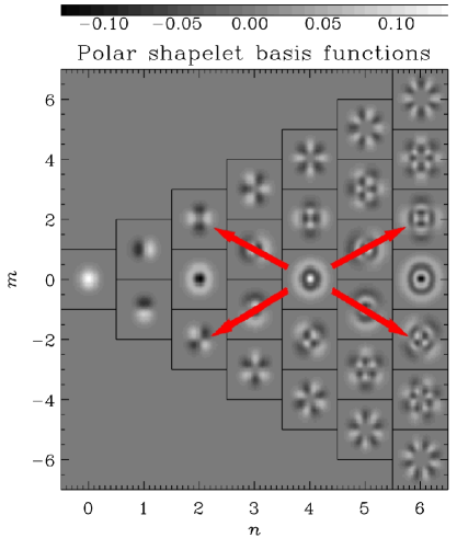
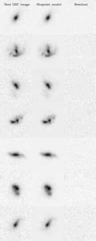
Figure 1: Left panel: Polar shapelet basis functions. These are complex functions: the real parts are shown in the top half ($m\geq 0$) of the plot, and the imaginary parts in the bottom half of the plot. The basis functions with $m=0$ are wholly real. In a shapelet decomposition, all of the basis functions are weighted by a complex number, whose magnitude determines the strength of a component and whose phase sets its orientation. Arrows indicate the “bleeding” of power into four adjacent shapelet coefficients when a small shear is applied. Right panel: Reconstruction of irregular HDF galaxies. Accurate models can be produced for even these peculiar shapes, using $n_{\rm max}$ between 12 and 15, to leave image residuals entirely consistent with noise.

The shapelets technique is based around the decomposition of a galaxy image $f(r,\theta)$ into a weighted sum of (complete) orthogonal basis functions

$$f(r,\theta)=\sum_{n=0}^{\infty}\sum_{m=-n}^{n}f_{n,m}\chi_{n,m}(r,\theta;\beta)~{},$$

where $f_{n,m}$ are the “shapelet coefficients”. The polar shapelet basis functions $\chi_{n,m}(r,\theta)$ are shown in figure 1. These are successive perturbations around a Gaussian of width $\beta$ (equivalent to $r_{g}$ in KSB), parameterised by indices $n$ and $m$. The mathematics of a shapelets is somewhat analogous to Fourier synthesis, but with a compact support well-suited to the modelling of localised galaxies. For example, a shapelet decomposition can similarly be truncated to eliminate the highly oscillatory basis functions that correspond noise in the original image.

Note that figure 1 takes a convenient shorthand form. The basis functions are only defined if $n$ and $m$ are both even or both odd but, for clarity, their images have been enlarged into the spare adjacent space. The polar shapelet basis functions and coefficients are also complex numbers. However, the constraint that a combined image should be a wholly real function introduces degeneracies: $f_{n,m}=f^{*}_{n,-m}$ and the coefficients with $m=0$ are wholly real. The top half of figure 1 with $m\geq 0$ shows the real parts of the basis functions; the bottom half $m<0$ shows the complex parts.

Before finding the shapelet coefficients for an image, it is necessary to specify the centre of the shapelet basis functions, and their scale size $\beta$. Since shapelets form a complete basis, decomposition is possible at any value of $\beta$. However, there is definitely a preferred scale for most galaxies, with which a faithful model can be produced using only a small number of shapelet coefficients. [Massey & Refregier (2004)] have written an algorithm to automatically decompose an arbitrary image into shapelets by exploring values of $\beta$. It seeks a model of the image that leaves a residual consistent with noise, and chooses the scale size that achieves that goal using the fewest coefficients. The optimal centre of the basis functions can be found simultaneously, by shifting the basis functions so that the model’s unweighted centroid is zero. The procedure can also deal analytically with the pixellisation of observational data, and perform deconvolution from a Point-Spread Function. Its success at faithfully modelling of even irregular HDF galaxies is demonstrated in the right-hand panel of figure 1. A complete IDL software package to implement the shapelets decomposition of arbitrary images, and to perform analysis and manipulation in shapelet space, can be downloaded from www.astro.caltech.edu/$\sim$rjm/shapelets/.

3 Why shapelets?

It would be, of course, possible to analyse images using a more physically motivated basis set, or traditional Sersic and Moffat radial profiles. However, the shapelet basis functions are specifically chosen to simplify image analysis and manipulation as encountered in weak gravitational lensing. As shown by [Massey & Refregier (2004)], shears, magnifications and convolutions are elegantly represented in shapelet space as the mixture of power between an (almost) minimal number of adjacent basis states. Shapelets are not motivated by their physics but rather their mathematics. The burden of proof for shapelets therefore shifts to the question of whether the central cusps and extended wings of real galaxies can be faithfully modelled by a set of functions based around a Gaussian. In fact, the recovery of galaxies’ extended wings is surprisingly complete with this algorithm. The process is helped by the fact that the smooth shapelets basis functions can find faint but coherent signal spread over many pixels, even though it may be beneath the noise level in any given pixel (and therefore not detected by SExtractor).

4 Interpreting a polar shapelet decomposition

A polar shapelet decomposition conveniently separates components of an image that are intuitively different. The index $n$ describes the total number of oscillations (spatial frequency) and also the size (radius) of the basis function. The index $m$ describes the degree of rotational symmetry of the basis functions.

Basis functions with $m=0$ are rotationally invariant. A circularly symmetric object contains power only in these states; its flux and radial profile are defined by the realtive values of its $m=0$ coefficients. An object containing only $m=0$ states will be a useful place to start for lensing analysis because, if galaxies’ intrinsic ellipticities are uncorrelated, the ensemble average of an unlensed population will indeed be circularly symmetric. Even in a typical galaxy, most of the power compactly occupies shapelet coefficients with low $m$, and particularly those with $|m|=0$ or 2.

Basis functions with $|m|=1$ are invariant only under rotations of $360^{\circ}$. These coefficients encode an object’s centroid: their real and imaginary parts correspond to displacements in the $x$ and $y$ directions. Alternatively, their moduli correspond to an absolute distance, and their phases indicate a direction.

Basis functions with $|m|=2$ are invariant under rotations of $180^{\circ}$, and become negative versions of themselves under rotations of $90^{\circ}$. These are precisely the properties of an ellipse. Indeed, an object’s Gaussian-weighted ellipticity $e\equiv e_{1}+ie_{2}$ is simply given by $f_{2,\pm 2}$. Its unweighted ellipticity is a combination of all of the $|m|=2$ shapelet coefficients. Ellipticity estimators can also incorporate coefficients with $|m|=6,10,14,...$, because their basis functions also contain at least the necessary symmetries.

5 The effect of weak gravitational lensing in shapelet space

All linear transformations can be described in shapelet space by the mixing of power between a few adjacent shapelet coefficients. For example, let us begin with an object containing power in just its $f_{4,0}$ coefficient. This is indicated by the arrows overlaid on figure 1. As the object is sheared by $\gamma\equiv\gamma_{1}+i\gamma_{2}$, this power “bleeds” into four nearby coefficients by an amount proportional to $\gamma$. Thus $f_{2,2}~{}\rightarrow~{}f_{2,2}~{}+~{}\gamma~{}\times~{}\mathrm{constant}~{}\times~{}f_{4,0}$ (recall that $f_{2,2}$ is complex). To first order, $f_{4,0}$ is unchanged. The diagonal pattern of the arrows is identical across the $n$ vs $m$ plane, although the constant varies as a function of $n$ and $m$. For more details, see [Massey & Refregier (2004)].

An initially circular object may contain power in all of its $m=0$ coefficients. After a small shear, it also contains power in its $|m|=2$ coefficients: the combination of circularly-symmetric plus quadrupole states produces an ellipse. Weak shear estimators primarily involve combinations of the $|m|=2$ shapelet coefficients. For example, the $f_{2,2}$ coefficient is the KSB ellipticity estimator. For a circularly symmetric object, this will have been affected under the shear by the initial values of $f_{0,0}$ and $f_{4,0}$. A weighted combination of these two (real) coefficients gives the trace of the KSB $P^{\gamma}$ shear susceptibility tensor (ignoring terms involving correction for PSF anisotropy).

A non-circularly symmetric object can also contain nonzero $|m|=4$ coefficients. Under a shear, the $f_{4,\pm 4}$ coefficients affect the $f_{2,2}$ coefficient (plus some $|m|=6$ coefficients) to order $\gamma^{*}$. Indeed, $f_{4,\pm 4}$ are the off-diagonal components of the KSB shear susceptibility tensor. Unfortunately, the complex conjugation of $\gamma$ mixes the $\gamma_{1}$ and $\gamma_{2}$ signals between the real and imaginary parts of the $f_{2,2}$. It becomes impossible to disentangle the two components of shear; and KSB can only work by averaging the shapes of many galaxies, to ensure that the population’s initial $|m|=4$ coefficients are precisely zero.

Using shapelets, every shapelet coefficient with $|m|=2$ can provide a statistically independent ellipticity estimator. Each of these has an effective $P^{\gamma}$ involving its adjacent $m=0$ and $|m|=4$ coefficients. Multiple shear estimators are very useful. Firstly, they can act as a consistency check to examine measurement errors within each object. They can also be combined to increase S/N: either by a simple average, or in more sophisticated ways that remove some of the biases of KSB (while staying stay linear in flux). For example, it is possible to take a linear combination of $|m|=2$ coefficents that is independent of the choice of $\beta$. However, the most successful estimator involves a “multiple multipole” combination of $|m|=2,6,10,\dots$ shapelet coefficients that has $P^{\gamma}={\rm flux}$. This is an exciting result for weak lensing, solving all of the problems with KSB’s $P^{\gamma}$ listed in §1. An object’s flux is its zeroth-order moment, which can be measured with less noise; it is a single, real number; and this shear susceptibility is unchanged by a (pure) shear. We can therefore form shear estimators using individual galaxies rather than having to average over a population ensemble. The method works stably for any galaxy morphology, because it does not rely on objects’ initially having zero $|m|=4$ coefficients. This is particularly important when the calibration is perfomed on simple image simulations using elliptical galaxies with concentric isophotes.

As a final note of caution, gravitational lensing does not apply a pure shear: it also applies a magnification, of the same order as $\gamma$. The enlargement caused by a lensing magnification mixes power between a small number of nearby shapelet coefficients. However, an enlargement is also equivalent to a increase of $\beta$: this effect is therefore eliminated from lensing measurements using a decomposition method with an adaptative choice of $\beta$. KSB and shapelet shear measurements are also insensitive to the flux amplification, because they are all formed from one linear sum of coefficients divided by another.

6 Results

To test (and calibrate) various shear measurement methods, we have created simulated images containing a known shear signal, $\gamma_{\rm in}$. We can then compare measured values to the true value. Our simulated images mimic the depth, pixellisation and PSF of the HDF, but the galaxies are simply parameterised by concentric ellipses with an exponential radial profile. Such objects are chosen to make the test especially challenging for shapelets-based methods: their central cusps and extended wings of such objects will be hard to match, while the concentric isphotes improve the prospects for KSB, that effictively measures shear at only one fixed radius. We have created many 7.5 square degrees simulated images, each containing a constant input signal in one component of shear, and zero in the other. Every shear measurement (and each point in figure 2) can therefore be performed as an average over a realistic population of galaxy sizes, magnitudes and intrinsic ellipticities.

The shear measured by a real KSB pipeline, $\gamma_{\rm measured}$, is shown in the left-hand panel of figure 2. Almost identical results can be reproduced using the shapelets software to imitate KSB. The statistical errors are quite large and there is calibration bias, as already noticed by [Bacon et al. (2001)]. The value of the calibration factor can vary as a function of exposure time and galaxy morphology, and therefore needs to be calibrated using realistic simulated images. The precision of the KSB method is therefore dependent upon the fidelity of the simulated images used to test it.

Using the shapelets formalism, we can derive many statistically independent shear estimators for each object. The middle panel of figure 2 shows their (noise-weighted) average. This does indeed have higher S/N than the KSB measurement; however, it still exhibits the familiar calibration bias. The right-hand panel of figure 2 shows results for the multiple multipole shear estimator. This is very sensitive to weak shears: indeed, a measurement of the components of shear that are not shown in figure 2 (which are all zero) gives 0.06%$\pm$0.10%. For large input shear values, $|\gamma_{\rm in}|>6$%, the precision of this shapelets-based shear estimator is also sufficient to detect deviations from the weak shear approximation.

7 Conclusions

A shapelet decomposition parameterises all of an object’s shape information, in a convenient and intuitive form. Several shear estimators can be formed from combinations of shapelet coefficients. These are not only more accurate than KSB, but also more stable. In particular, the use of higher order moments to analytically remove any calibration factor reduces the reliance of older methods upon simulated images to faithfully model all aspects of observational data.

Figure 2: Left panel: recovery of a known shear signal using KSB. Errors are at the $\sim 10$% level. The calibration bias has to be measured using simulated images, then corrected for in real data. Middle panel: shear recovery by combining shapelet coefficients to create multiple, KSB-like estimators. The S/N improves, but the calibration bias remains. Right panel: shear recovery using a more sophisticated, “multiple multipole” shapelets-based shear estimator. This is precise enough to detect deviations from the weak shear approximation at high values of $|\gamma_{\rm in}|$.