Weak Lensing by Large-Scale Structure with the FIRST Radio Survey

Abstract

We present the first measurement of weak lensing by large-scale structure on scales of $1-4$ degrees based on radio observations. We utilize the FIRST Radio Survey, a quarter-sky, 20 cm survey produced with the NRAO Very Large Array (VLA). The large angular scales afforded by the FIRST survey provide a measurement in the linear regime of the matter power spectrum, thus avoiding the necessity of applying uncertain non-linear corrections. Moreover, since the VLA interferometer has a well-known and deterministic beam, our measurement does not suffer from the irreproducible effects of atmospheric seeing which limit ground-based optical surveys. We use the shapelet method described in an earlier paper to estimate the shear from the shape of radio sources derived directly from the interferometric measurements in the Fourier($uv$) plane. With realistic simulations we verify that the method yields unbiased shear estimators. We study and quantify the systematic effects which can produce spurious shears, analytically and with simulations, and carefully correct for them. We measure the shear correlation functions on angular scales of $0.5^{\circ}-40^{\circ}$, and compute the corresponding aperture mass statistics. On $1^{\circ}-4^{\circ}$ scales, we find that the B-modes are consistent with zero, and detect a lensing E-mode signal significant at the 3.0$\sigma$ level. After removing nearby radio sources with an optical counterpart, the $E$-mode signal increases by 10-20%, as expected for a lensing signal derived from more distant sources. We use the E-mode measurement on these scales to constrain the mass power spectrum normalization $\sigma_{8}$ and the median redshift $z_{m}$ of the unidentified radio sources. We find $\sigma_{8}(z_{m}/2)^{0.6}\simeq 1.0\pm 0.2$ where the $1\sigma$ error bars include statistical errors, cosmic variance, and systematics. This is consistent with earlier determinations of $\sigma_{8}$ from cosmic shear, the cosmic microwave background (CMB) and cluster abundance, and with our current knowledge of the redshift distribution of radio sources. Taking the prior $\sigma_{8}=0.9\pm 0.1$ (68%CL) from the WMAP experiment, this corresponds to $z_{m}=2.2\pm 0.9$ (68%CL) for radio sources without optical counterparts, consistent with existing models for the radio source luminosity function. Our results offer promising prospects for precision measurements of cosmic shear with future radio interferometers such as LOFAR and the SKA.

1. Introduction

Weak gravitational lensing by large-scale structure, or ‘cosmic shear’, has emerged as a powerful tool for measuring the mass distribution of the Universe (see van Waerbeke & Mellier 2003; Refregier 2003 for recent reviews). This effect is based on the distortion induced in the images of background galaxies by the gravitational tidal field of the intervening large-scale structure. Since light rays from nearby background galaxies travel through similar mass inhomogeneities along the way, the resulting image distortions are correlated. By measuring the coherent lensing distortions of background galaxies, one can thus probe the mass distribution projected along the line of sight. The underlying physics is well-understood, and the observational signatures can be directly compared to theoretical predictions. The distortion depends on the mass fluctuations, as well as on the mean mass density of the Universe. Since it is a projected effect, the amplitude is also sensitive to the geometry of the Universe and on the background source distribution in redshift space.

The lensing distortion can be quantified by a $2\times 2$ tensor field, parameterized by the convergence and shear parameters, with the latter being the direct observable. Since galaxies have an intrinsic shape distribution, the shear signal must be measured statistically, assuming galaxies are on average randomly oriented. The lensing effect of interest here is not associated with any specific mass concentrations, but is measured by sampling random regions of the sky. The typical amplitude of the shear in this regime is only on the order of a few percent on arcminute scales, and is therefore challenging to measure. Large areas of the sky must be surveyed to reduce statistical errors, and systematic effects that spuriously distort the shape of the observed sources need to be carefully corrected for.

The theoretical basis for cosmic shear was pioneered by Gunn (1967), and was further elaborated in a modern cosmology language by, e.g., Blandford et al. (1991), Miralda-Escude (1991), Kaiser (1992, 1998), Jain and Seljak (1997), and Schneider (1998). Because of its challenging observational nature, cosmic shear was firmly detected for the first time only recently (Bacon et al. 2000; Kaiser et al. 2000; van Waerbeke, et al. 2000; Wittman et al. 2000). Since then, the cosmological origin and implications of the shear signal have been rapidly established by many more groups (most recently Bacon et al 2003; Brown et al. 2003; Hamana et al. 2003; Hoekstra et al. 2002; Jarvis et al. 2003; Refregier et al. 2002; van Waerbeke et al. 2002). Collectively, the shear two-point statistics have been measured from $\theta\sim 1^{\prime}$ to $100^{\prime}$ angular scales, spanning the non-linear ($\theta\lesssim 10^{\prime}$) and quasi-linear ($\theta\gtrsim 10^{\prime}$) regime of the matter power spectrum, and are consistent with predictions from the popular $\Lambda$CDM model. Constraints on the matter density $\Omega_{m}$ and the power spectrum normalization $\sigma_{8}$ from different cosmic shear measurements are broadly in agreement with one another, and are roughly consistent with measurements from the cluster abundance method (e.g., Pierpaoli et al. 2001; Seljak 2002).

Until now, all current cosmic shear measurements have been performed in the optical and near-infrared bands, with similar observational and analysis techniques. Here, we report a cosmic shear measurement using the FIRST Radio Survey (Becker et al. 1995; White et al. 1997). FIRST is a quarter-sky radio survey at 1.4 GHz conducted using the Very Large Array (VLA) in its B-configuration, and therefore provides a unique measurement of the mass power spectrum on large angular scales (Kamionkowski et al. 1998; Refregier et al. 1998; Chang & Refregier 2002). Radio surveys like FIRST offer several advantages for cosmic shear. Firstly, unlike optical galaxies, bright radio sources are typically at high redshifts, thereby increasing the path-length to each through the Universe, and thus the strength of the lensing signal. Secondly, the VLA is a radio interferometer and thus has a well-known and deterministic beam, allowing for modeling of crucial systematic effects to high accuracy. In contrast, ground-based optical surveys are limited by the irreproducible effects of atmospheric seeing. Finally, FIRST is a sparsely-sampled but wide-angle survey, well-suited for measurements in the linear part of the mass power spectrum. This avoids the theoretical uncertainties arising from the non-linear corrections of the mass power spectrum required to interpret the optical cosmic shear surveys that are sensitive to smaller scales.

To deal with the important issue of accurate shear measurements and systematics corrections, we use the shapelet method described in Chang & Refregier (2002, hereafter CR02; see also Refregier 2003b; Refregier & Bacon 2003) to measure the shape and shear information from interferometric data directly in Fourier space. The method is linear and yields unbiased shear estimators. Systematic effects such as instrumental distortions can be closely modeled.

Our paper is organized as follows. In §2 we describe the theoretical background and notations for cosmic shear. In §3, we summarize the main features of the FIRST radio survey and the properties of its radio sources. In §4, we describe briefly our shape measurement method, discussing the impact of systematic effects in §5. The systematics corrections are described in §6. In §7, we present our results for the measurement of cosmic shear, and discuss their cosmological implications. Our conclusions are summarized in §8.

2. Theory

We first briefly describe the theoretical basis of cosmic shear and the statistics we will use to present our results (see, e.g., Bartelmann & Schneider 2000 for a review).

2.1. Weak Lensing

In a weakly inhomogeneous FRW Universe, light rays from distant sources are deflected by the gravitational tidal field of intervening structures. In the weak-lensing limit, the resulting distortion and magnification can be quantified by a $2\times 2$ tensor field, $\psi_{lm}$, which, following from the geodesic equation, can be related to the gravitational potential $\Phi$:

$$\psi_{lm}={2\over c^{2}}\int d\chi g(\chi)\partial_{l}\partial_{m}\Phi$$ (1)

where the radial window function $g(\chi)$ is defined as

$$g(\chi)=r(\chi)\int_{\chi}^{\chi_{h}}d\chi^{\prime}n(\chi^{\prime}){r(\chi^{\prime}-\chi)\over r(\chi^{\prime})}.$$

Here, $n(\chi^{\prime})$ is the normalized source redshift distribution, $r(\chi)$ is the comoving angular-diameter distance, $\chi$ is the radial comoving coordinate, and $\chi_{h}$ corresponds to the horizon. The comoving derivatives $\partial_{i}$ are perpendicular to the line-of-sight. The symmetric distortion tensor $\psi_{lm}$ can be parameterized by the convergence, $\kappa$, and the shear $\gamma_{1}$ and $\gamma_{2}$. These are defined as

$$\kappa = {1\over 2}(\psi_{11}+\psi_{22})$$ (2)

$$\gamma_{1} = {1\over 2}(\psi_{11}-\psi_{22}),~{}~{}~{}\gamma_{2}=\psi_{12}=\psi_{21}$$ (3)

Adding to Equation (2) a $\psi_{33}$ term which cancels out upon $\chi$ integration, and using Poisson’s equation in the form of $\nabla^{2}\Phi={3H_{0}^{2}\Omega_{m}\over 2a}\delta$, one relates the convergence field $\kappa$ to the density fluctuation $\delta$, weighted by the window function $g(\chi)$. Applying Limber’s equation in Fourier-space, the power spectrum of convergence, $P_{\kappa}$, can then be expressed in terms of the 3-D mass power spectrum, $P_{\delta}$ (e.g., Kaiser 1992) as

$$P_{\kappa}(l)={9H_{0}^{4}\Omega_{m}^{2}\over 4c^{4}}\int_{0}^{\chi_{h}}d\chi\left[{g(\chi)\over a(\chi)r(\chi)}\right]^{2}P_{\delta}\left({l\over r(\chi)};\chi\right)$$ (4)

where $\delta$ is the mass-density fluctuation, $a(\chi)$ is the cosmological scale factor, and $H_{0}$ and $\Omega_{m}$ are the present-day Hubble constant and matter density parameter, respectively. Note that the convergence and shear fields are related by (e.g., Kaiser & Squires 1993)

$$\kappa=\partial^{-2}\partial_{i}\partial_{j}\gamma_{ij},$$ (5)

where $\partial^{-2}$ is the inverse 2D Laplacian operator

$$\partial^{-2}\equiv{1\over 2\pi}\int d^{2}\hat{r}\ln|\hat{r}-\hat{r^{\prime}}|.$$ (6)

In the flat sky approximation, the convergence power spectrum is equal to the shear power spectrum $P_{\gamma}=P_{\kappa}$. The shear power spectrum is simply related to other 2-point shear statistics which are more convenient in practice and which we describe below.

2.2. Shear Correlation Functions

For each pair of galaxies, we define the tangential and $45^{\circ}$-rotated shear components, $\gamma_{t}$ and $\gamma_{r}$, with respect to the great circle connecting the two galaxies: as

$$\gamma_{t} = \gamma_{1}\cos(2\theta)+\gamma_{2}\sin(2\theta)$$

$$\gamma_{r} = \gamma_{2}\cos(2\theta)-\gamma_{1}\sin(2\theta),$$ (7)

where $\theta$ is the position angle between the x-axis and the great circle. In analogy to the CMB polarization correlations, one can then construct coordinate-independent correlations from the rotated shear components (Kamionkowski et al. 1998). There are three independent pair-wise shear correlation functions, $C_{1}(\theta)=\langle\gamma_{t}(\theta_{0})\gamma_{t}(\theta_{0}+\theta)\rangle$, $C_{2}(\theta)=\langle\gamma_{r}(\theta_{0})\gamma_{r}(\theta_{0}+\theta)\rangle$, and $C_{3}(\theta)=\langle\gamma_{t}(\theta_{0})\gamma_{r}(\theta_{0}+\theta)\rangle$. The first two correlation functions are related to the shear power spectrum (e.g., Miralda-Escude 1991)

$$C_{1}(\theta) = \int{ldl\over 4\pi}P_{\gamma}(l)[J_{0}(l\theta)+J_{4}(l\theta)]$$

$$C_{2}(\theta) = \int{ldl\over 4\pi}P_{\gamma}(l)[J_{0}(l\theta)-J_{4}(l\theta)],$$ (8)

while the parity invariance of weak lensing ensures that $C_{3}(\theta)$ vanishes. The measurement of a non-zero $C_{3}(\theta)$ is, therefore, an indication of a non-lensing contribution, such as that from residual systematics.

2.3. $M_{ap}$ Statistics

The aperture mass is defined as (Kaiser 1995; Schneider et al. 1998)

$$M_{ap}(\theta)=\int_{|{\mathbf{\phi}}|<\theta}d^{2}{\mathbf{\phi}}U(|{\mathbf{\phi}}|)\kappa(\phi),$$ (9)

where $U(\phi)$ is a compensated filter defined so that $\int_{0}^{\theta}d\phi~{}\phi U(\phi)=0$, and $\kappa(\phi)$ is the convergence field. The $M_{ap}$ statistic thus measures the spatially-filtered projected density field, and can be conveniently related to the shear as

$$M_{ap}(\theta)=\int_{|{\mathbf{\phi}}|<\theta}d^{2}{\mathbf{\phi}}Q(|{\mathbf{\phi}}|)\gamma_{t}(\phi),$$ (10)

where $Q(\phi)={2\over\phi^{2}}\int_{0}^{\phi}d\phi^{\prime}\phi^{\prime}U(\phi^{\prime})-U(\phi)$, and $\gamma_{t}$ is the rotated tangential shear, as in Eq.(2.2), with respect to the aperture center. The aperture mass variance is related to the shear power spectrum by (Schneider et al. 1998):

$$\langle M_{ap}^{2}(\theta)\rangle={288\over\pi\theta^{4}}\int{dl\over l^{3}}P_{\gamma}(l)[J_{4}(l\theta)]^{2}.$$ (11)

The $M_{ap}$ statistic has the advantage that the mass density can be directly obtained from the observables – the shear – without the need for mass reconstruction. The weight function $Q$ is relatively narrow in Fourier space, so that the $M_{ap}(\theta)$ measurements do not strongly correlate. As a result, $M_{ap}(\theta)$ and $M_{ap}(2\theta)$ are almost independent of each other. Note that $M_{ap}(\theta)$ probes the scale of $\sim\theta/4$ (Schneider 1998).

Weak gravitational lensing arises from scalar perturbations to the space-time metric, and therefore the shear field is expected to possess no handedness. One can decompose the shear tensor field into gradient (E-mode) and curl (B-mode) components (Stebbins 1996). The gradient part contains the weak lensing signal, while the curl part is expected to be zero. Gravitational waves produce non-zero B-mode signals, but their effect is expected to be very small. Thus, the B-mode provides a useful check for any non-lensing contaminations, such as residual systematic effects or intrinsic shape correlations (e.g., Heavens 2001). A rotation of 45 degrees in the aperture brings a curl-free field to a curl field, and also transforms a tangential shear to a radial shear component. Thus, the B-mode of the aperture mass, $M_{\bot}$, is simply

$$M_{\bot}(\theta)=\int_{|{\mathbf{\phi}}|<\theta}d^{2}{\mathbf{\phi}}Q(|{\mathbf{\phi}}|)\gamma_{r}(\phi),$$ (12)

where $\gamma_{r}(\phi)$ is the radial shear with respect to the aperture center. The aperture mass statistic therefore provides a convenient way for E- and B-mode decomposition, and can be computed directly from the observed shear.

The aperture mass variance can also be expressed in terms of the shear correlation functions. Defining

$$C_{+}(\theta)=C_{1}(\theta)+C_{2}(\theta);~{}~{}C_{-}(\theta)=C_{1}(\theta)-C_{2}(\theta),$$ (13)

the aperture masses are given by

$$\langle M_{ap}^{2}(\theta)\rangle = {1\over 2}\int_{0}^{2\theta}{\phi d\phi\over\theta^{2}}[C_{+}(\phi)T_{+}({\phi\over\theta})+C_{-}(\phi)T_{-}({\phi\over\theta})]$$

$$\langle M_{\bot}^{2}(\theta)\rangle = {1\over 2}\int_{0}^{2\theta}{\phi d\phi\over\theta^{2}}[C_{+}(\phi)T_{+}({\phi\over\theta})-C_{-}(\phi)T_{-}({\phi\over\theta})],$$

where the functions $T_{+}$ and $T_{-}$ are defined in Schneider, van Waerbeke & Mellier (2002).

3. Data

3.1. FIRST Survey

The FIRST radio survey (Becker et al. 1995; White et al. 1997) was conducted at the NRAO Very Large Array (VLA) at 1.4 GHz in the B configuration. The survey is the radio equivalent of the Sloan Digital Sky Survey covering $\sim 10,000$ deg² of the Northern Galactic Cap. It consists of 3-minute snapshots covering a hexagonal grid using 14 3-MHz frequency channels. Its $5\sigma$ flux density limit is 1 mJy, with a restoring beam FWHM of $5^{\prime\prime}.4$. The survey contains $\sim 9\times 10^{5}$ sources, roughly 40% of which are resolved. The basic source information is described in the on-line FIRST catalog (http://sundog.stsci.edu/).

3.2. Redshift Distribution

For our weak lensing measurement, the source redshift distribution determines the weight function along the line of sight, and thus conditions the strength of the lensing signal. The signal depends most strongly on the source median redshift $z_{m}$ and somewhat on the redshift distribution. As discussed below, the redshift distribution for radio sources is rather uncertain, and we have therefore considered $z_{m}$ as a free parameter throughout the paper.

For our purposes, we consider the redshift distribution for radio sources estimated by Dunlop & Peacock (1990; hereafter DP). These authors estimated the radio luminosity functions (RLF) for the steep- and flat-spectrum sources at 2.7 GHz, using faint sources with optical counterparts in the UGC catalog and the Parkes selected regions database with source flux densities $>100$ mJy. They presented seven redshift models, with model 7 considered with two cases: mean- and high-redshift source distributions. The former have assigned redshifts that are the mean values for galaxies of a given K-band luminosity, and the latter have redshifts larger than the average, to account for a possible bias.

The normalized differential redshift distribution of the DP models is shown in Fig. 1. The RLF’s were integrated over luminosities that produce flux densities greater than 1 mJy. The DP models were shifted to 1.4 GHz for computation, assuming a spectral index of $\alpha=-0.85$ for steep-spectrum sources and $\alpha=0$ for flat-spectrum sources, where $L\propto\nu^{\alpha}$. The DP model 1 is the fundamental model, and models 2 to 5 are variations relative to it. For clarity, only the averaged values of models 2 to 5 are shown. The high redshift end was truncated at $z=4.5$, as models 4 and 5 have unphysical spikes at $z\sim 6$. Model 7 includes effects of source evolution in luminosity and density, and is considered the most probable approximation (Magliocchetti et al. 1999). The spike near $z=0$ is due to starburst galaxies; however, optical follow-up observations suggest the spike is probably unphysical (Magliocchetti et al. 2000). The vertical bars show the median redshifts for each model (truncated at $z=4.5$) which range from $z_{m}\sim 0.9$ to $1.4$.

Figure 1.— Normalized differential redshift distribution of the FIRST radio sources using the models by Dunlop and Peacock (1990, DP). The DP model 1, the average of models 2-5, and models 7 with the mean and high-redshift estimations are shown. The vertical lines indicate the median redshifts of each model.

4. Shear Measurement

4.1. Shapelet Method

We summarize the relevant components of the shapelet method described in CR02. In this approach, the surface brightness $f({\mathbf{x}})$ of an object is decomposed as

$$f({\mathbf{x}})=\sum_{{\mathbf{n}}}f_{{\mathbf{n}}}B_{{\mathbf{n}}}({\mathbf{x}};\beta),$$ (15)

where the Fourier transform of the basis functions are given by

$$B_{{\mathbf{n}}}({\mathbf{x}};\beta)\equiv\frac{H_{n_{1}}(\beta^{-1}x_{1})~{}H_{n_{2}}(\beta^{-1}x_{2})~{}e^{-\frac{|x|^{2}}{2\beta^{2}}}}{\left[2^{(n_{1}+n_{2})}\pi~{}\beta^{2}~{}n_{1}!~{}n_{2}!\right]^{\frac{1}{2}}}$$ (16)

representing the two-dimensional orthonormal Gauss-Hermite basis functions of characteristic scale $\beta$, where $H_{m}(\xi)$ is the Hermite polynomial of order m, ${\mathbf{x}}=(x_{1},x_{2})$ and ${\mathbf{n}}=(n_{1},n_{2})$. In practice, the series only include a finite number of terms with order $n_{1}+n_{2}\leq N_{\rm max}$.

The decomposition and its applications have also been studied by Refregier (2003), Refregier & Bacon (2003) and independently by Bernstein & Jarvis (2002). The bases are complete and yield fast convergence in the expansion if $\beta$ and $x=0$ are close to the size and location of the object, respectively. The basis functions can be thought of as perturbations around a two-dimensional Gaussian, so that the coefficients are the Gaussian-weighted moments of the source. The basis functions are also the eigenfunctions of the Quantum Harmonic Oscillator. Under a linear coordinate transformation, such as a weak shear, the basis functions have analytic responses, making an unbiased shear estimator easy to construct from the coefficients. Furthermore, the basis functions are their own Fourier transforms up to a rescaling factor (see Eq. 18 below), and are thus localized functions in both real and Fourier spaces. They are thus convenient for analyzing data from interferometers, which measure the Fourier-transform of the sky surface brightness.

Making use of the basis functions, we model the source intensity directly in the Fourier (or $uv$) space, where the FIRST interferometric data (visibilities) are collected. The Fourier transform $\tilde{f}_{s}({\mathbf{k}})$ of object intensity $f_{s}(l,m)$ of each source $s$ is a sum of the Fourier shapelets basis functions

$$\tilde{f}_{s}({\mathbf{k}})=\sum_{\mathbf{n}}f_{{\mathbf{n}}s}\tilde{B}_{\mathbf{n}}({\mathbf{k}}-{\mathbf{k}}_{s};\beta_{s}^{-1}),$$ (17)

where

$$\widetilde{B}_{{\mathbf{n}}}({\mathbf{k}};\beta^{-1})=i^{(n_{1}+n_{2})}B_{{\mathbf{n}}}({\mathbf{k}};\beta).$$ (18)

A $\chi^{2}$ fit is used to simultaneously model all sources in the field:

$${\chi}^{2}=({\mathbf{V}}-{\mathbf{M}~{}f})^{T}~{}{\mathbf{C}}^{-1}~{}({\mathbf{V}}-{\mathbf{M}~{}f}),$$ (19)

where ${\mathbf{V}}=\{\overline{V}_{c}\}$ is the binned visibility data vector, ${\mathbf{M}}=\{\overline{B}_{c}^{{\mathbf{n}}s}\}$ is the theory matrix whose components are the basis functions of different order ${\mathbf{n}}$ evaluated at the respective source ${\mathbf{k}}_{s}$, and ${\mathbf{f}}=\{f^{{\mathbf{n}}s}\}$ is the coefficient vector for all sources. We assume the data error matrix ${\mathbf{C}}$ is diagonal and constant, ${\mathbf{C}}=\sigma^{2}{\mathbf{I}}$, where $\sigma$ is the noise level and ${\mathbf{I}}$ the identity matrix; this is a reasonable approximation for the VLA observations since the noise of antennas is independent. To find the best-fit solution, we solve a set of simultaneous least-squares equations. The covariance matrix of the best-fit coefficients ${\mathbf{f}}$ is then

$$W({\mathbf{f}})=\sigma^{2}({\mathbf{M}}^{T}{\mathbf{M}})^{-1},$$ (20)

which provides an estimate of the errors on the coefficients and can be used to compute the errors of derived quantities, such as source flux density and size, and the shear estimator. In §4.2 below, we explain how the shapelet centroid, scale $\beta$, and maximum order $N_{\rm max}$ are chosen in practice.

An unbiased shear estimator for each source and for each shapelet order $n$ is then given by (Refregier & Bacon 2003)

$$\hat{\gamma}_{n}=\frac{4}{[n(n+2)]^{\frac{1}{2}}}\frac{\hat{f}_{n,2}}{\langle\hat{f}_{n-2,0}-\hat{f}_{n+2,0}\rangle}$$ (21)

where $\hat{\gamma}=\gamma_{1}+i\gamma_{2}$ is the complex shear, and the brackets denote an average over an unlensed object ensemble. The coefficients $\hat{f}_{n,m}$ are the complex polar shapelet coefficients which are related to the Cartesian coefficients of equation (15) by a simple linear transformation (see Refregier 2003b). In this paper, we will only consider the $n=2$ shear estimator $\hat{\gamma}_{2}$, which captures most of the shape information of faint radio sources. The error on the shear estimator can be straight-forwardly propagated from the covariance matrix.

4.2. Choice of Shapelet Parameters

One issue which needs to be resolved is the choice of the shapelet parameters – $\beta$, $N_{\rm max}$ and centroid – for each source. The shapelets centroid was simply chosen to match the source centroid position in R.A. and Dec. listed in the FIRST catalog, converted into $l,m,n$ coordinates.

To generate this conversion, we note that the R.A. and Dec. coordinate system, also called the $x,y,z$ coordinate system, is fixed to the Earth. It is defined so that the $x,y$ axes define the plane of the equator and the $z$ axis points along the rotation axis of the Earth. The $l,m,n$ system is identical to the $u,v,w$ system, and is defined, for a given pointing, so that the $w$ axis points towards the phase tracking center and the $u$ axis is in the $x,y$ plane. Let $h$ and $\delta$ be the hour angle and declination of a source. Its coordinate in the $x,y,z$ system is then $x=\cos\delta\cos h,y=-\cos\delta\sin h,z=\sin\delta$. The corresponding coordinates in the $u,v,w$ coordinate system are then given by

$$\left(\begin{array}[]{c}l\\ m\\ n\end{array}\right) = \left(\begin{array}[]{ccc}\sin h_{0}&\cos h_{0}&0\\ -\sin\delta_{0}\cos h_{0}&\sin\delta_{0}\sin h_{0}&\cos\delta_{0}\\ \cos\delta_{0}\cos h_{0}&-\cos\delta_{0}\sin h_{0}&\sin\delta_{0}\\ \end{array}\right)$$ (32)

$$\times\left(\begin{array}[]{c}\cos\delta\cos h\\ -\cos\delta\sin h\\ \sin\delta\end{array}\right),$$

where $h_{0}$ and $\delta_{0}$ are the hour angle and declination of the phase tracking center for this pointing. If the source is at the phase tracking center ($h=h_{0},\delta=\delta_{0}$), the position on the $u,v,w$ system is ${\mathbf{l}}=(0,0,1)$, as expected since $l,m,n$ are directional cosines such that $l^{2}+m^{2}+n^{2}=1$. For small displacements $h=h_{0}+\Delta h,\delta=\delta_{0}+\Delta\delta$ away from the phase tracking center, the $l,m$ position takes the familiar form ${\mathbf{l}}\simeq{\mathbf{l}_{1}}=(-\Delta h\cos h_{0},\Delta\delta,1)$ to first order in the displacement.

The choice of $\beta$ and $N_{\rm max}$ is important to ensure that each source is faithfully modeled, that the shapelet series converges, and that our shape measurement is unbiased. To study the first two issues, we ran a series of simulated grid pointings with the observing conditions of FIRST, as described in CR02. The input sources are described by elliptical Gaussians with major axes, minor axes, and position angles taken from the FIRST catalog. Note that this choice of source model is simplistic and facilitates the convergence of the shapelet series. This is however the standard model used in radio astronomy to parameterize radio sources. In particular, this parameterization is adopted by the source fitting software used to generate the FIRST catalog, and is therefore a natural model to use for our simulations. This choice may affect the exact values of beta and $N_{\rm max}$ derived, but it will not bias our final shear estimator as long as these parameters are within the acceptable range (see Figure 2). In CR02, we tested our shapelet reconstruction algorithm in detail and found that it also performs well for more complicated source models.

With these simulation, we then considered a series of values of $\beta$ and $N_{\rm max}$ for one of the sources in the pointing, while keeping these parameters constant for the other sources (all centroids were also kept fixed). We also added in noise in the $uv$ plane, and studied the behavior of sources with different SN ratios. The added noise level is equal to 0.15 mJy per beam in real space, which is the typical noise level for FIRST. The lowest SN ratio considered is 5, which corresponds to the FIRST detection limit; we explored over two orders of magnitudes of SN ratios, covering the range appropriate for FIRST sources. From the reconstructed images, we find a moderately narrow range of parameters which yield sensible reconstructions. To quantify this range, we computed the $\chi^{2}$ difference between the input image $f_{\rm in}({\mathbf{l}})$ and the fitted image $f_{\rm fit}({\mathbf{l}}_{p};\beta,N_{\rm max})$ defined as

$$\chi^{2}\equiv\frac{\sum_{p=1}^{N_{\rm pix}}\left[f_{\rm fit}({\mathbf{l}}_{p};\beta,N_{\rm max})-f_{\rm in}({\mathbf{l}}_{p})\right]^{2}}{\sigma^{2}_{f{\rm in}}N_{\rm pix}},$$ (33)

where the sum is over all $N_{\rm pix}$ pixels within a radius of $5\beta$ about the centroid. For convenience, $\chi^{2}$ was normalized by the rms $\sigma_{f{\rm in}}$ of the pixel distribution of $f_{\rm in}$.

An example of the resulting dependence of $\chi^{2}$ on $\beta$ and $N_{\rm max}$ is shown in Figure 2, where the SN ratio was set to a high value of 500 in this case. The range of acceptable parameter values is reflected as the region with $\chi^{2}\sim 1$ on the figure, showing that $\chi^{2}$ is a good measure of the reconstruction. In this case, the best reconstruction is near $(\beta,N_{\rm max})=(1.5,4)$. In the presence of noise, the best reconstruction tends to favor smaller $N_{\rm max}$ values while leaving the best $\beta$ unchanged.

We have repeated the above procedure for various sources in different simulated FIRST grids. This allowed us to relate the optimal $\beta$ and $N_{\rm max}$ values to the major and minor axes of the sources derived from the elliptical Gaussian fits listed in the FIRST catalog. We thus derived an empirical relation between the observed shape parameters in the FIRST catalog (the deconvolved major and minor axes) and the optimal shapelets parameters ($\beta$ and $N_{\rm max}$) for the source ensemble: $\beta=\sqrt{0.9\times(a/2.35)\times(b/2.35)}$, and $N_{\rm max}=a/1.5-1$, where $a$ and $b$ denote the FWHM of the major and minor axes. This ’recipe’ was then applied to the real sources in the FIRST survey.

To test the implementation of this recipe in our shear measurement method, we have performed further simulations. Elliptical Gaussian sources were first generated with source parameters following the distribution of the real sources in the FIRST catalog. These artificial sources were then sheared with a constant 5% value for both $\gamma_{1}$ and $\gamma_{2}$. The corresponding visibilities with the FIRST survey settings were generated for over 1,000 simulated pointings with $\sim 30-40$ sources per pointing. We then used the above recipe to determine the shapelet parameters, and applied the method described in CR02 to calculate the shapelet coefficients for the $\sim$ 30,000 synthetic sources. The estimators for $\gamma_{1}$ and $\gamma_{2}$ of each source were then calculated according to Eq. (21) applied to different flux-size bins. We find that the input shear amplitudes are accurately recovered within the $1\sigma$ statistical errors. We also performed a null simulation (with zero shear) and verified that the resulting shear measurement was consistent with zero.

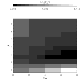
Figure 2.— Dependence of the shapelet reconstruction on the shapelet parameters $\beta$ and $N_{\rm max}$. The color scale shows the $\chi^{2}$ difference between simulated image parameters and their shapelet reconstruction values, as defined in Eq. (33). Only a small range of $\beta$ and $N_{\rm max}$ values are acceptable and yield good reconstructions. For small $\beta$ values, an increasing $N_{\rm max}$ value quickly result in poor reconstructions.

4.3. Implementation

Given a set of FIRST flux- and phase-calibrated $uv$ data, sources positioned within a radius of $64^{\prime}$ from the phase center are selected from the FIRST Catalog. This large radius limit ensures bright sources in the primary beam side lobes are also included in the simultaneous fit and thus do not contaminate the fainter sources within the primary beam. Sources which are separated by less than $20^{\prime\prime}$ are merged into one source, as simulations show that treating close companions as one source yields the best shapelet fits (see also the discussion in §5.6). The shapelet parameters are determined according to the prescription described in §4.2. We then compute the source shapelet coefficients and their covariance matrix using a least-squares fit to the visibilities, where all sources in a given pointing are fitted simultaneously. In principle, some of the systematics that distort the shape of sources could be corrected for at this stage. However, to save computing time, we decided to correct for the systematics afterwards, as described in the next section. The whole FIRST data set observed up to year 2001 were processed on the UK Cosmos Supercomputer. The total of about 50,000 individual pointings required about 9,000 hours of Cosmos CPU time.

As a first check, the output coefficients were examined by computing the source fluxes and centroids derived from the shapelet coefficients (see CR02). Along with those fields flagged when the fit failed to converge, we have discarded about $3\%$ of the processed sources, due to corrupted observational data, numerical convergence problems and, in a few cases, inadequate choice of input shapelet parameters. On average, the computed shapelet flux densities and centroids agree rather well with those in the FIRST catalog, which used an elliptical Gaussian fit to measure source intensities and positions. The shapelet flux densities and flux density errors were then combined to compute the signal-to-noise ratio of each source. To control systematics, we discarded measurements with observing parameters $|HA|>4$ hours and $\sqrt{l^{2}+m^{2}}>20^{\prime}$, and only kept sources with an integrated flux density $\geq$ 1mJy and deconvolved major axis $<7^{\prime\prime}$. Excluding the measurements for point sources (deconvolved major axis $<2^{\prime\prime}$), we thus were left with $\sim 3.6\times 10^{5}$ usable shear estimators with associated measurement errors.

Since the FIRST pointings partially overlap (see Becker et al. 1995 for details), each source is observed from one to four times. We verified that the corrected shear estimators of a given source in different pointings are consistent within the errors. The shear estimators of a given source are then coadded using the square of the observed signal-to-noise ratio as a weight. The sky coverage in the northern cap is close to 8000 $\deg^{2}$, and the resulting resolved (major axis $>2^{\prime\prime}$ and $<7^{\prime\prime}$) source number density is about 20 sources $\deg^{-2}$.

5. Summary of Systematic Effects

Because the weak-lensing signal is only on the order of 1%, systematic effects must be carefully accounted for, as they may otherwise introduce spurious shear correlations. The dominant systematics arise from the anisotropy of the synthesized beam, which is directly related to the $uv$ sampling, and thus on the geometry of the interferometric array. Note that, unlike the case with optical observations, systematic effects in our case are well-known and deterministic (albeit somewhat complicated) and can be calculated to high-degree of accuracy. In the following, we briefly describe the different sources of systematic effects and show that they are best viewed as functions of four observing parameters (see e.g., Perley et al. 1989; Taylor et al. 1999; & Thompson et al. 1986 for a detailed description of these effects).

5.1. The HA-DEC Effect

Interferometric data are collected in Fourier space, or $uv$ space, at a finite and discrete number of points. The Fourier-transform of the sky surface brightness is thus multiplied by the $uv$ sampling function which determines the shape and size of the convolution beam (PSF) in real-space. The $uv$ sampling function is deterministic and is a sum of delta functions centered on the positions

$$\left(\begin{array}[]{c}u\\ v\\ w\end{array}\right) = {1\over\lambda}\left(\begin{array}[]{ccc}\sin H&\cos H&0\\ -\sin\delta\cos H&\sin\delta\sin H&\cos\delta\\ \cos\delta\cos H&-\cos\delta\sin H&\sin\delta\\ \end{array}\right)\left(\begin{array}[]{c}L_{x}\\ L_{y}\\ L_{z}\end{array}\right),$$ (43)

where $\lambda$ is the observing wavelength, $(L_{x},L_{y},L_{z})$ are the VLA antenna spacings, and $H$ and $\delta$ are the source hour-angle and declination. Since the former two are fixed and known for a given observation, the effective beam can thus be calculated exactly from the source position on the sky. This can be seen as the projection of the antenna plane onto the $uv$ plane, which depends on the source position.

With the knowledge of the $uv$ sampling function, we place a point source at the phase-tracking center and generate simulated visibilities using the FIRST observing settings. The simulated visibilities are modeled using the Shapelet method, and the artificial shear of the simulated source due to systematics are calculated using the fitted Shapelet coefficients. We then repeat the procedure for various values of $(H,\delta)$. The resulting shape distortion is shown in Fig 3. The distortion is minimal at small hour angles and at declination near 34 degrees, corresponding to the latitude of the VLA, when sources are directly overhead. The induced distortion is $\sim 5\%$ at $(H,\delta)=(3.5^{hr},-5^{\circ})$, roughly in the radial direction with respect to $(H,\delta)=(0,34^{\circ})$.

Figure 3.— The artificial shear pattern induced by the HA-DEC effect. The length and direction of the plotted lines indicate the amplitude and orientation of the distortion, respectively. The line at the bottom-left indicates a distortion of 5%.

5.2. The Non-coplanar Effect

The VLA is a two-dimensional array laid out across the surface of the Earth. Due to the curvature and rotation of the Earth, the visibilities are not strictly measured in a plane but in the three-dimensional Fourier space labeled as $(u,v,w)$:

$$V(u,v,w) = \int\int{dldm\over\sqrt{1-l^{2}-m^{2}}}I(l,m)\times$$ (45)

$$e^{-2\pi i[ul+vm+w(\sqrt{1-l^{2}-m^{2}}-1)]},$$

where for simplicity we have ignored other systematic effects which we describe below. For short observing durations and for sources close to the phase tracking center, the $w$ term is small and is often dropped. In this approximation the visibility function reduces to a two-dimensional Fourier transform

$$V(u,v)=\int\int{dldm\over\sqrt{1-l^{2}-m^{2}}}I(l,m)e^{-2\pi i[ul+vm]},$$ (46)

which has the advantage of allowing fast computation. This approximation induces a distortion of the source images that depends on the amplitude of $|w(\sqrt{1-l^{2}-m^{2}}-1)|$, i.e., on the distance from the phase tracking center $(l=0,m=0)$. As mentioned in the previous section, the amplitude of $w$ depends on the source observing hour angle and declination. Thus, the shape distortion due to the two-dimensional approximation is a function of the source position $(l,m)$ with respect to the phase center, as well as the observing hour angle and declination. In our Shapelet approach, we use the two-dimensional approximation in order to save computing time, and therefore the distortion must be corrected for.

We quantify this distortion using simulations similar to that described in §5.1, but with sources placed at various off-center positions in the simulated grid using equation (45). Fig. 4 shows an example of the resulting distortion pattern, for which the simulated source is placed at ($l$,$m$)=$(7^{\prime},7^{\prime})$. In this setting, the distortion at $(H,\delta)=(0^{hr},-5^{\circ})$ is $\sim 20\%$, and is roughly in the radial direction with respect to$(H,\delta)=(0,34^{\circ})$. This effect is the dominant source of systematic effects (see §6.2).

Figure 4.— The artificial shear pattern induced by the non-coplanar effect, for the case of $(l,m)=(7^{\prime},7^{\prime})$ away from the phase-tracking center. The line at the bottom-left indicates a distortion of 45%.

5.3. Bandwidth Smearing

The bandwidth-smearing effect with interferometers is exactly analogous to chromatic aberration in an optical telescope. It is due to the fact that radio interferometric observations are not monochromatic, but are instead done within a finite frequency band. As a result, the visibility registered at a particular $uv$ position is actually an average of the actual visibilities over a small interval of $(u,v)$ positions extended in the radial direction. The delay tracking, which corrects for the difference in arrival time of light rays at two antennas prior to correlation of the signals, is only accurate at the center of the field-of-view and at the central observing frequency. Suppose that the observing central frequency is $\nu_{0}$ and the phase tracking center is $(l_{0},m_{0})$. Signals at frequency $\nu$ arriving from sky position $(l,m)$ will have a phase delay error of $(u_{0}l+v_{0}m)/\nu_{0}$, resulting in a phase shift of $2\pi(\nu-\nu_{0})(u_{0}l+v_{0}m)/\nu_{0}$. The smeared visibilities, $\tilde{V}$, are thus (Perley et al. 1994)

$$\tilde{V}(u_{0},v_{0}) = {1\over\int d\nu^{\prime}G(\nu^{\prime})}\int d\nu^{\prime}V\left(u_{0}{\nu\over\nu_{0}},v_{0}{\nu\over\nu_{0}}\right)({\nu\over\nu_{0}})^{2}$$ (47)

$$\times~{}G(\nu^{\prime})e^{2\pi i{\nu^{\prime}\over\nu_{0}}(u_{0}l+v_{0}m)},$$

where $G(\nu)$ is the passband function and $\nu^{\prime}=\nu-\nu_{0}$. For simplicity, here and in the following, we ignore the effect of the primary beam power pattern and the weighting function in the $uv$ plane. In real space, this corresponds to a convolution of the true sky intensity, $I(l,m)$, with a distortion function $D$, such as $\tilde{I}(l,m)=I(l,m)\ast D(l,m,\nu)$, where $D$ is defined as

$$D(l,m,\nu^{\prime})=\int\int du_{0}dv_{0}e^{2\pi i(u_{0}l+v_{o}m)}\times~{}~{}~{}~{}~{}~{}~{}$$

$$\left[{1\over\int d\nu^{\prime}G(\nu^{\prime})}\int d\nu^{\prime}G(\nu^{\prime})e^{2\pi i{\nu^{\prime}\over\nu_{0}}(u_{0}l+v_{0}m)}\right],$$ (48)

provided that the fractional bandwidth is sufficiently small. The amplitude of bandwidth-smearing distortion therefore depends on the source position (with respect to the phase tracking center), and on the size of the frequency interval. Since a change in frequency moves the $uv$ points radially on the $uv$ plane, bandwidth smearing distorts the observed images in the radial direction with respect to the field center.

For FIRST, $G(\nu)$ can be approximated by a square passband with a width of 3 MHz. The distortion induced $20^{\prime}$ away from the center of the field-of-view is about 6%. The resulting shear pattern is shown in Figure 5.

Figure 5.— The artificial shear pattern induced by the bandwidth smearing effect. The length and direction of the plotted lines indicate the amplitude and orientation of the distortion, respectively.

5.4. Time Averaging

Time-averaging smearing is another systematic effect that results from data averaging. Correlated signals received by pairs of antennas are, in practice, averaged over small time intervals in order to reduce the size of the visibility files. During a time-interval $\delta t$, the Earth rotates by an angle of $\omega_{e}\delta t$, where $\omega_{e}$ is the Earth angular rotation velocity. For observations at a declination of $90^{\circ}$, the Earth rotation corresponds to a tangential rotation in the $uv$ plane. The true visibilities are therefore averaged over an interval of $uv$ positions, extended tangentially, which results in a tangential distortion of images in real space. The time-averaging effect at declination $90^{\circ}$ thus bears an interesting analogy to the bandwidth smearing effect, which distorts images in the radial direction.

In general, however, the time averaging effect is more complex. Depending on the source position relative to the antenna (Earth) space, the loci on the $uv$ plane over which visibilities are being averaged varies in length and shape. A convenient way to estimate the size of image distortion is to calculate the response of a point source. Since the time averaging effect preserves the integrated flux density, the induced tangential broadening must be compensated for by the reduction in the peak amplitude of the point source response.

Averaging a waveform of frequency $\nu$ over a time interval $\delta t$ reduces the amplitude of the response by sinc$(\nu\delta t)\approx 1-(\pi\nu\delta t)^{2}/6$, for $\nu\delta t\ll 1$, where $\nu\delta t$ corresponds to the phase change. For a source at $(l,m)$ with respect to the phase-tracking center, the instantaneous phase rate is $({du\over dt}l+{dv\over dt}m)$, and therefore, integrating over a small time interval $\delta t$, the reduction of the amplitude of the point source response is

$$R_{\delta t}={I\over I_{0}}\approx 1-{\pi^{2}{\delta t}^{2}\over 6}\left({du\over dt}l+{dv\over dt}m\right)^{2},$$ (49)

where

$${du\over dt} = {\omega_{e}\over\lambda}(L_{x}\cos H-L_{y}\sin H)$$

$${dv\over dt} = {\omega_{e}\over\lambda}(L_{x}\sin\delta\sin H+L_{y}\sin\delta\cos H),$$ (50)

which follows directly from Equation (43), and $\omega_{e}={dH\over dt}$.

Combining the above two equations, we can estimate the reduction of response for sources at any given observing coordinates $(H,\delta)$. The amplitude of the tangential width broadening due to time-averaging smearing is then simply $R_{\delta t}^{-1}$. The distortion is therefore a function of the antenna configuration ($L_{x}$ and $L_{y}$), the source position in the sky (the hour angle and declination), and the source position with respect to the center of the field-of-view $(l,m)$.

For FIRST, the averaging time-interval is five seconds. The resulting distortion pattern for $\delta=90^{\circ}$ in shown in Figure 6. The distortion from time averaging smearing is small in the FIRST settings; for most sources the distortion is less than 0.1%.

Figure 6.— The artificial shear pattern induced by the time-averaging smearing effect for the case of $\delta=90^{\circ}$. The distortion pattern is tangential in this case. The pattern varies with sky position, but in general, the distortion is on the order of 0.1% at the edge of the field-of-view of concern.

5.5. Primary Beam Attenuation

In practice, the true sky surface brightness $I(l,m)$ is multiplied by the antenna power pattern of the primary single dish $A(l,m)$ before signals are correlated. The primary beam power pattern is closely related to the diffraction pattern of a circular dish, and can be approximated by (Condon et al. 1998)

$$A(r)=\left({2J_{1}({r\over r_{0}})\over r/r_{0}}\right)^{2},$$ (51)

where $J_{1}$ is the Bessel $J$ function of order 1, $r\simeq 3.23\times\sqrt{l^{2}+m^{2}}$, and $r_{0}$ is the FWHM of the primary beam pattern. For FIRST, $r_{0}=30^{\prime}.83$.

The primary beam pattern introduces a variation in sensitivity in the radial direction across the observing field-of-view which modifies the observed shape of source images. A general treatment of this effect is detailed in the Appendix. The effect depends on the primary beam power pattern as well as on the source sizes; for larger sources the distortion is more severe. Using Equations (51) and (A6), we calculate the effect for typical FIRST sources. The distortion is in the radial direction with respect to the field center, and the induced shear pattern for a circular Gaussian source with FWHM of $10^{\prime\prime}$ ($\sim 2$ times the beam size) is shown in Fig 7. The distortion is less than 0.01% and thus the effect can be safely ignored in the FIRST case.

Figure 7.— The artificial shear pattern induced by the primary beam power pattern attenuation. The resulting distortion is radial and very small. For a big circular Gaussian source with a FWHM of $10^{\prime\prime}$, the distortion is less than 0.01%.

5.6. Source Fragmentation

A significant fraction of radio sources have a double-lobe structure, and are often broken into two components by the FIRST object finder. Because these radio lobes tend to be aligned, this produces strong shear correlations on small angular scales. As mentioned in §4.3, we have treated sources within $20^{\prime\prime}$ of each other, the typical separation of double-lobe sources, as a single source for the shapelet fitting. Furthermore, for sources that lie within $1^{\prime}$, only one source is selected at random for use in the shear measurements. This leads to a loss of information only on scales smaller than $1^{\prime}$, a scale much smaller than the scales on which we measure the weak lensing signal (greater than about $30^{\prime}$; see §7 below)

Figure 8.— (a) The shear pattern in the HA-DEC plane from the averaged shear measurements. The line at the bottom left corner indicates an amplitude of 10% shear. (b) The shear pattern in the HA-DEC plane from the simulated shears due to the systematic effects. The line at the bottom left corner indicates an amplitude of 10% shear.

Figure 9.— (a) The shear pattern in the $l$-$m$ plane from the averaged shear measurements. The line at the bottom left corner indicates an amplitude of 3% shear. (b) The shear pattern in the l-m plane from the simulated shears due to the systematic effects. The line at the bottom left corner indicates an amplitude of 3% shear.

6. Corrections for Systematics

6.1. Observations

Without correction, the shear measurements of our FIRST sample are dominated by the systematic effects described above. These effects are complicated and are correlated with each other, and can not easily be decomposed into convolutions and distortions, as is the case with optical observations. To correct them, we therefore adopt a statistical approach by measuring and subtracting the systematic shear as a function of the observation parameters (RA, DEC, l, m) and of the source size. As a test, we also apply the same procedure to the simulations.

Figs. 8a and 9a show the average of the shear estimators for each of the $\sim 5.3\times 10^{5}$ measurements (with major axis $>2^{\prime\prime}$ and $<17^{\prime\prime}$ before coaddition) in HA-DEC and l-m bins for all source sizes. Since the lensing signal averages out in these cells (see §6.4 for more details), the resulting patterns give a measure of the systematics.

The HA-DEC plane shows a large-scale pattern in $15\times 6$ degree bins. Most (75%) of the measurements concentrate in the central two HA columns, $|HA|<1$, which have the highest statistical accuracy. The shear pattern in the l-m plane is less prominent, and shows a predominantly vertical pattern. The measurements are more evenly distributed in this plane, although the number density decreases at larger radii. Note that all measurements with $|HA|>4$hrs and $\sqrt{l^{2}+m^{2}}>20^{\prime}$ have been excluded at an earlier stage. The systematics shown in these two planes are coupled: the minimum shear distortion occurs at around $HA=0$, Dec $\simeq 34^{\circ}$, where sources are directly overhead from the VLA, and at the phase tracking center $l=0,m=0$. The farther away from these two central values, the greater the spurious shear due to systematics. We also examined the dependence of the systematics on the source size cuts, and found that smaller sources are subject to larger systematic distortions, as expected. We do not find any significant dependence on observation epoch over the eight years of the observing campaign.

Figure 10.— (a) The shear correlation function of the data without correction for the systematics. The error bars are computed from field-to-field variations, and include statistical errors and cosmic variance. (b) The shear correlation function of the simulations without corrections for the systematics. The 1-$\sigma$ error bars are computed from field-to-field variations.

6.2. Simulations

As discussed in §5, the largest systematic distortions for FIRST are the coupled HA-DEC and non-coplanar effects, which produce as much as $\sim$ 50% artificial shear when a source combines low declination, with an observation at large hour angle, and at a position far from the phase tracking center. Another important contribution is from the bandwidth-smearing effect, which produces $\sim$ 6% shear $20^{\prime}$ from the phase tracking center. Although the systematic effects are well-understood and calculable to high accuracy, their impact on the shear statistics is complicated, since source observations do not uniformly occupy the HA-DEC-l-m space and since we apply complicated cuts during the analysis.

Ideally, we could use a control sample, such as point sources, to quantify the systematic effects and check our correction method. Since point sources carry no lensing information, any measured shear must indeed be due to systematic effects. However, in our shapelets approach, the shear estimators require fitting coefficients up to $n=4$ (Eq. 21), which is a poor choice of input parameter for point sources (see, e.g., Fig. 2). This not only compromises the fits for point sources, but also affects the reconstruction of resolved sources, since all sources in a given field are fitted simultaneously. Although we could imagine increasing the size of $\beta$ for point sources to yield a more reasonable fit, this would be difficult to implement given the presence of other sources (leaving aside the problem of quantifying the effects on these sources). In addition, this would have meant doubling the fitting parameters in the model and thus doubling the computing time, which was already substantial. More importantly, the systematic effects can in fact be understood and calculated very accurately, as we will see below. The averaged data described in the previous section also serves as another check for systematics. To quantify the systematics at the required precision, we therefore have carried out further simulations to study the impact on the shear statistics.

For this purpose, we consider the HA-DEC, non-coplanar, and bandwidth-smearing effects and ignore the other effects, which are at least one order of magnitude smaller in amplitude, or have been incorporated directly in the analysis (such as the source fragmentation effect). Using the FIRST Catalog, we begin by randomizing the source position angles, which, along with the major and minor axis information, gives a measure of the intrinsic ellipticity distribution. For every source, we computed the combined systematic distortions listed above for each individual observation; the result is subsequently convolved with the source’s intrinsic shape and multiple observations are coadded. To avoid large computing time, we calculated the systematics on a grid in HA-DEC-l-m space, and interpolate between the grid positions. Examples are shown in Figs. 8b and 9b, where we average the simulated measurements in the same HA-DEC and l-m bins as for the observations. The resulting shear patterns and amplitudes are almost identical to those of the data (see Figs. 8a and 9a excepting for the l-m patterns which show small discrepancies at the edges of the field where the data are of low statistical significance. We are therefore confident that the systematics estimation is, at least on average, a good representation of the true systematics for individual sources.

Figure 11.— (a) The shear pattern from the averaged shear measurements after the HA-DEC corrections. The line at the bottom left corner indicates an amplitude of 1% shear. (b) The shear pattern from the simulated shears after the HA-DEC corrections. The line at the bottom left corner indicates an amplitude of 1% shear.

6.3. Uncorrected Shear Correlation Functions

We compute the rotated shear correlation functions, $C_{1}$, $C_{2}$, and $C_{3}$, as described in §2, for both the simulation and the data. Operationally, the shear correlation functions are measured as

$$C_{1}(\theta) = {\sum_{i,j}w_{i}w_{j}\gamma_{t}({\bf\theta}_{i})\gamma_{t}({\bf\theta}_{j})\over\sum_{i,j}w_{i}w_{j}}$$

$$C_{2}(\theta) = {\sum_{i,j}w_{i}w_{j}\gamma_{r}({\bf\theta}_{i})\gamma_{r}({\bf\theta}_{j})\over\sum_{i,j}w_{i}w_{j}}$$ (52)

where the sums are over all pairs of galaxies i and j, and $\theta=|{\bf\theta}_{i}-{\bf\theta}_{j}|$ is the separation of pairs within a bin. Similarly, for $C_{3}$, the $\gamma$’s are replaced by $\gamma_{t}({\bf\theta}_{i})$ and $\gamma_{r}({\bf\theta}_{j})$, respectively. We adopt the optimal weight function derived by Bernstein & Jarvis (2002)

$$w={1\over\sqrt{\gamma^{2}+(1.5\sigma_{\eta})^{2}}},$$ (53)

where $\sigma_{\eta}$ is the measurement uncertainty in each shear component, as measured by the Shapelet method, and transformed to the sheared coordinates in which the shape is circular. We divide the data into twelve subsamples according to their sky position, and compute the correlation functions separately. The correlation functions are calculated in bins of $\Delta\ln(\theta)=0.2$, and the 1-$\sigma$ error bars are quantified using the field-to-field variation of the twelve subsamples. The error bars include noise from uncertainties in the shape measurements, from cosmic variance, and from intrinsic dispersion of the (unlensed) source shapes, which by averaging over the entire sample is measured to be around $\sim 0.4$.

The data shear correlation functions, without any corrections, are heavily dominated by the systematics, and we expect their correlation functions to have high amplitude and to appear similar to those of the simulation. As demonstrated in Figs. 10a and 10b, the general behaviors of the $C_{1}$ and $C_{2}$ functions for the data and of the simulation are in very good agreement from $10^{\prime}$ to $40^{\circ}$. For the $C_{3}$ function, the simulation captures the large-scale behavior well but does less well on small angular scales. It is nevertheless reassuring that our knowledge of the systematics is realistic.

Note that the measurements of $C_{1}$ and $C_{2}$ on different angular scales in Fig.10 appear correlated both for the data and for the simulations. This reflects the fact that the systematics, which dominate $C_{1}$ and $C_{2}$ before the corrections, are strongly correlated within a patch of the sky used to measure the correlation functions. On the other hand, $C_{3}$ (for $\theta\lesssim 1000^{\prime}$) is less correlated, and therefore its errors are dominated by statistical uncertainties.

Figure 12.— (a) The shear correlation function of the data after HA-DEC corrections.The lines over-plotted indicate predictions from the $\Omega_{m}=0.3$ $\Lambda$CDM model, with $\sigma_{8}=0.9$, and source redshifts lying on the plane of $z_{m}=1,1.5,2,2.5$, respectively. (b) The shear correlation functions of the simulation after HA-DEC corrections. The corrections follow the exact same procedure as the corrections to the data. The lines show the $\Lambda$CDM predictions as in (a).

6.4. Corrected Shear Correlation Functions

First, let us re-examine the averaged shear pattern on the HA-DEC plane (Fig. 8a). It is evident that this large-scale pattern is contributed almost entirely by systematics. Using the averaged data, we fit a two-dimensional 2nd-order polynomial to this plane, and subsequently subtract the fitted systematics from individual sources. The sources are grouped according to their sizes and observed l-m position in the field for the modeling and the corrections. We have tried both polynomial fits and spline fits to the systematics and find that the resulting residuals are comparable. The residual shear pattern is shown in Fig. 11 and appears small in amplitude and random in orientation, as desired. We discard measurements with averaged residual shear values greater than 1.5% in all following analyses. To test for our control of the systematics, we perform the same procedure with the simulated shears; the residual shear pattern is random and very small in amplitude.

We then study the shear correlations function after the HA-DEC corrections for both the data and the simulation. As shown in Fig. 12a, the amplitudes of the data $C_{1}$ and $C_{2}$ correlations are an order-of-magnitude smaller than those of the uncorrected data (Fig. 10a), and the high amplitude tail of $C_{3}$ on large angular scales seen before the correction has disappeared. The shear correlation functions of the simulation are also well-behaved on large angular scales, but have much smaller amplitudes between 10 and $100^{\prime}$ (see Fig. 12b).

The correction for the $l$-$m$ dependence is more complicated. After source coaddition, which depends on the declination of the phase center and the number of times a source was observed, for most sources the $l$-$m$ shear pattern roughly cancels out, while for others it is enhanced or distorted. This is potentially a contamination to the lensing signal that is difficult to isolate and correct for. We nevertheless perform a correction on the $l$-$m$ plane similar to that for the HA-DEC plane. First, we examine the shear pattern on the $l$-$m$ plane using observed and simulated shears that have been corrected for the HA-DEC pattern, fit a low-order polynomial to the plane, and then subtract the fitted pattern from individual measurements. The sources are grouped according to their size for modeling and corrections, and measurements with averaged residual shear values greater than 1.5% are discarded. After corrections and coaddition, we again compute the correlation functions for both the data and the simulation. Interestingly, the correlation functions are almost identical to those that have been corrected for HA-DEC patterns only; i.e., the $l$-$m$ pattern correction does not alter the correlation functions of the data or of the simulation. We also checked our corrections by considering subsamples with different source sizes and did not find significant differences in the resulting correlation functions.

We also ran a further series of correlation function tests. We consider using only sources within $15^{\prime}$ of the phase-tracking center where the $l$-$m$ distortions are small, excluding sources at low declination ($<10^{\circ}$) where the combined HA-DEC and $l-m$ distortions are severe, relaxing or strengthening our imposed constraints on excluding source close companions (discarding sources within $5^{\prime\prime}$ to $60^{\prime\prime}$ of one another), and changing the range in major axes of the selected sources. Remarkably, the shear correlation functions of the data and of the simulation remain very similar to those of Figs. 12a and 12b, respectively, in every case.

We therefore conclude that the HA-DEC corrected shear correlation functions are fairly robust, and that the systematics dependence on the four parameters, HA, DEC, $l$ and $m$ are well-reproduced by the simulations. We thus take the simulated shear correlation functions after HA-DEC corrections, which are non-zero on most scales, as our best estimation for the residual systematics in the HA-DEC and $l$-$m$ parameter space. To correct for these, we subtract the residual simulated $C_{1}$ and $C_{2}$ correlation functions from the corresponding data correlation function. The errors in each correlation function are then added in quadrature.

7. Results

7.1. $M_{ap}$ Statistics

Using the shear correlation functions $C_{1}(\theta)$ and $C_{2}(\theta)$ measured above, we compute the $M_{ap}$ 2-point statistics using Eq. (2.3). The variances $\langle M_{ap}^{2}\rangle$ and $\langle M_{\perp}^{2}\rangle$ contain the E-mode and B-mode, respectively, and are plotted in Fig. 13 as a function of aperture radius $\theta$. While the E-mode displays a significant signal, the B-mode amplitude is consistent with 0 on all scales. The scale dependence of the E-modes for $\theta\gtrsim 200^{\prime}$ is consistent with that expected for the $\Lambda$CDM model (see curves), but deviates from this model on smaller scales. The $M_{ap}$ statistics with an aperture radius of $\theta$ is mostly sensitive to angular scales of about $\theta/4$. The depleted E-modes may therefore reflect the presence of systematics on scales smaller than $50^{\prime}$, which roughly corresponds to the scale of the individual fields ($40^{\prime}$ in diameter). This could be due to an over- or under-correction of one or several of the systematic effects discussed in section §6.4.

In addition to the checks described in §6.4, we divided the data into high- and low-latitude halves, and east and west hemispheres, and computed again the $M_{ap}$ statistics in each case; the results are consistent with that of Fig. 13: the lensing signals are not confined to any particular part of the sky. Similarly, we separated the sources into two groups according to the observed flux density; again, the $M_{ap}$ statistics do not differ significantly. As a comparison, the $M_{ap}$ statistics computed from the simulations are shown in Fig. 14. The E- and B-modes of the simulation are consistent with zero on most scales, as expected, with the exception of slightly negative E-mode values on scales smaller than $\sim 200^{\prime}$ ($50^{\prime}$ in real space). This suggests a possible contamination from systematics on small angular scales, as discussed above.

In order to test for the presence of a lensing signal on scales larger than $50^{\prime}$, we removed FIRST sources for which an optical counterpart could be identified in the APM catalog (McMahon & Irwin 1992), which amounts to 10% of the FIRST sample. Excluding quasars, which are both rare and mostly point sources (all of which are excluded from our source sample), the redshifts of the APM sources peak at around $z\sim 0.15$ and are for the most part bounded by $z\lesssim 0.3$ (McMahon et al. 2002). By excluding them, we increase the median redshift of the source sample and thus expect the lensing signal to increase. Fig. 15 shows the $M_{ap}$ statistics for this new sample. The E-mode signal has a significance of $3.6\sigma$, as measured at the $\theta\sim 450^{\prime}$ scale. Compared to Fig. 13, the E-mode signal on scales $300^{\prime}\lesssim\theta\lesssim 700^{\prime}$ is indeed larger by 10-20%. This confirms the presence of the lensing signal on these scales.

As an interesting exercise, we calculate the median redshift derived from the DP redshift models (see §3.2) by excluding the $z<0.3$ region; the various median redshifts shown in Fig. 1 increase by about 10-15%. Since the $M_{ap}$ lensing signal increases roughly as $z_{m}^{2}$ to first order, the changes in the measured lensing signal wrought by the exclusion of the low-redshift sources is consistent with that expected from the consequent change in the estimated $z_{m}$ from the models.

Figure 13.— $M_{ap}$ statistics as a function of aperture radius $\theta$. The top panel shows the E-mode variance $\langle M_{ap}^{2}\rangle$, while the bottom panel shows the B-mode variance $\langle M_{\perp}^{2}\rangle$. The curves indicate predictions from the $\Omega_{m}=0.3$ $\Lambda$CDM model, with $\sigma_{8}=0.9$, $\Gamma=0.21$, and several source median redshifts $z_{m}$.

Figure 14.— Same as the previous figure, but the $M_{ap}$ statistics are computed using the simulations, which serve as a null test.

Figure 15.— Same as Fig. 13, but this time for only those sources lacking optical counterparts in the APM catalog.

7.2. Cosmological Implications

Using the $M_{ap}$ statistics from the sample without optical counterparts, we fit cosmological models to our data by computing the $\chi^{2}$ values:

$$\chi^{2}=({\mathbf{d}}-{\mathbf{m}})^{T}{\mathbf{W}}^{-1}({\mathbf{d}}-{\mathbf{m}}),$$ (54)

where ${\mathbf{d}}$ is the $M_{ap}$ data vector, ${\mathbf{m}}$ is the $\Lambda$CDM model vector and ${\mathbf{W}}$ the covariance matrix. For ${\mathbf{d}}$ we use the $M_{ap}$ values with $\theta>200^{\prime}$, thus avoiding sub-pointing scales which have unreliable systematics correction (see discussion above). The covariance matrix is computed from the field-to-field variations as described in §6.3 and is given by

$$W_{ij}={\Sigma_{n}({d_{i}}_{n}-\langle d_{i}\rangle)({d_{j}}_{n}-\langle d_{j}\rangle)\over N(N-1)},$$ (55)

where the sum is over different subsamples $n$, and $N=12$ is the total number of subsamples. The $d_{i}$’s are the $M_{ap}$ E-mode values at different scales, and $\langle d_{i}\rangle$ is their average over all 12 fields. Since the B-modes quantify the contamination from systematics and are consistent with zero at the selected angular scales, we add the B-mode covariance to the E-mode covariance matrix. As a result, the covariance matrix accounts for all the sources of errors, namely, intrinsic source shapes, shape measurement errors, cosmic variance, and systematics.

The data points from angular scales $200^{\prime}<\theta<1000^{\prime}$ are partially degenerate and contain only 3-4 independent measurements. We therefore use a singular value decomposition to calculate ${\mathbf{W}}^{-1}$, and discard the singular values of ${\mathbf{W}}$ which are negligible compared to the rest. Since the $M_{ap}$ data vector was initially computed at small angular intervals, we only keep four data points which contain the highest signal-to-noise ratios and are independent.

The redshift distribution of our sample is rather uncertain, as indicated by the various models for the radio source redshift-distribution discussed in §3.2. We therefore chose to vary two parameters in our fit: $\sigma_{8}$, the mass power spectrum normalization in spheres of $8h^{-1}$ Mpc, and $z_{m}$, the median source redshift. We assumed a $\Lambda$CDM model with fixed values of $\Omega_{m}=0.3$ and $\Gamma=0.21$. Note that, although we are probing scales greater than $8h^{-1}$ Mpc, the parameter $\sigma_{8}$ is convenient for comparing our results with those from other groups and methods.

The resulting $\chi^{2}$ contour plot is shown in Fig. 16. The solid contours indicate the 68.3%, 95.4% confidence levels from FIRST, excluding the predominantly low-redshift objects with APM optical counterparts. For comparison, the dashed contours show the 68.3% CL constraint from the FIRST sources including those with the APM counterparts which, as expected, are consistent with lower $z_{m}$ values. As a check, we used the linear power spectrum and the fitting formula from Smith et al. (2003) and Peacock & Dodds (1996), and found the contours do not vary appreciably. This is expected since we are probing the linear part of the mass power spectrum. To a good approximation, the contours (excluding APM counterparts) correspond to

$$\sigma_{8}\left(\frac{z_{m}}{2}\right)^{0.6}\simeq 0.95\pm 0.22,$$ (56)

where the 68%CL error includes statistical errors, cosmic variance, and systematic effects.

Recent cosmic shear measurements in the optical band yield values of $\sigma_{8}$ between 0.7 and 1.0 for $\Omega_{m}\simeq 0.3$ and $\Gamma\simeq 0.21$ (Bacon et al. 2003; Brown et al. 2003; Hamana et al. 2003; Hoekstra et al. 2002; Jarvis et al. 2002; Massey et al. 2003; Refregier, Rhodes, & Groth 2002; Rhodes, Refregier & Groth 2004; van Waerbeke et al. 2002). The averaged constraint from several of these surveys is $\sigma_{8}=0.83\pm 0.04$ (as compiled by Refregier 2003) for the same values of $\Omega_{m}$ and $\Gamma$. The constraint, $\sigma_{8}=0.9\pm 0.1$ (68%CL), from the WMAP CMB experiment (Spergel et al. 2003) is also shown in Fig. 16. For source redshifts in the range $1.4\lesssim z_{m}\lesssim 3.4$, our results are consistent (within $1\sigma$) with both of these different measurements. Reversing the argument and taking the WMAP determination of $\sigma_{8}$ as a prior, we find that the median redshift of the radio sources in our sample (without APM counterpart) is $z_{m}=2.2\pm 0.9$ at 68%CL. This redshift range is also consistent with the models for the radio source redshift distribution described in §3.2.

Figure 16.— Constraints on the spectrum normalization, $\sigma_{8}$, and on the source median redshift, $z_{m}$, from our FIRST cosmic shear measurement. The solid lines indicate the 68% and 95% CL from FIRST, excluding the predominantly low-redshift objects with APM optical counterparts. The dashed lines are the 68% CL from FIRST including sources with the APM counterparts. A $\Lambda$CDM model with $\Omega_{m}=0.3$ and $\Gamma=0.21$ was assumed. Also shown for comparison is the constraint from the WMAP CMB experiment $\sigma_{8}=0.9\pm 0.1$ (68%CL; Spergel et al. 2003).

8. Conclusions

We have presented our cosmic shear measurement using the FIRST Radio Survey over 8,000 square degrees of sky. We apply the shear measurement method described in Chang & Refregier (2002) to measure shear directly in Fourier space, where interferometric data are collected. In this shapelets approach, we carefully determined the input parameters for the source shape decomposition, and verified that the shear estimators are unbiased and robust using realistic simulations. The dominant systematic effects associated with interferometric observations were studied in detail. The analytical and simulated expectations of the systematics compared well with the data when considered functions of four observational parameters. We corrected the systematics both in this parameter space and in the correlation function domain, and verified the accuracy of the corrections with further simulations.

Using the corrected shear correlation functions, we computed the aperture mass statistic, which decomposes the signal into E- and B-modes, containing the lensing signal and the non-lensing contributions, respectively. We find that the B-modes are consistent with 0 on all scales considered, while the E-modes displays a significant lensing signal. The E-mode signal has a significance of $3.0\sigma$, as measured at the $\theta\sim 450^{\prime}$ scale. The signal increases by 10-20% when sources with optical counterparts (and, therefore, predominantly at low redshift) are excluded. This confirms the presence of a lensing signal which is expected to increase as the mean source redshift increases.

Using the E-mode $M_{ap}$ statistics on scales $200^{\prime}<\theta<1000^{\prime}$ (corresponding to physical scales from about $1^{\circ}$ to $4^{\circ}$) , we constrained jointly the power spectrum normalization $\sigma_{8}$ and the median redshift $z_{m}$ of our radio source sample. We find $\sigma_{8}(z_{m}/2)^{0.6}\simeq 1.0\pm 0.2$ where the $1\sigma$ error bars include statistical errors, cosmic variance and systematics. A $\Lambda$CDM model with $\Omega_{m}=0.3$ and $\Gamma=0.21$ was assumed. This result is consistent with earlier determinations of $\sigma_{8}$ from cosmic shear, and with the WMAP CMB experiment and cluster abundance tests. Taking the prior on $\sigma_{8}$ from the WMAP experiment, this corresponds to $z_{m}=2.2\pm 0.9$ (68%CL) for radio sources without optical counterparts, consistent with existing models for the radio source luminosity function.

Our shear measurement is complementary to the earlier cosmic shear results which were all performed in the optical or near-IR band. It is the first measurement using radio sources observed with interferometers and is therefore subject to very different systematic effects. We used a new shear measurement method which allows direct computation of shear estimators in Fourier space. Moreover, our measurement probes large angular scales, which are in the linear regime of structure growth, eliminating the need for uncertain non-linear corrections in the matter power spectrum. Our measurement thus offers promising prospects for measuring cosmic shear with future radio interferometers such as LOFAR and SKA, which offer exciting opportunities for precision measurements of cosmological parameters (Schneider 1999).

Appendix A Effect of Sensitivity Variations on Source Shapes

In general, the sensitivity of the image is not exactly constant across the image. Here, we compute the effect of the sensitivity variations on the shapes of sources. We then apply our results to the case of a radial primary beam pattern affecting a circular Gaussian source.

Let $i({\mathbf{x}})$ be the intrinsic intensity of a source as a function of position ${\mathbf{x}}$ on the image. The observed intensity is $i^{\prime}({\mathbf{x}})=i({\mathbf{x}})s({\mathbf{x}})$, where $s({\mathbf{x}})$ is the sensitivity function. In the application below, $s({\mathbf{x}})$ is simply the primary beam function. The true centroid ${\mathbf{x}^{0}}$ of the source is defined by

$${\mathbf{x}^{0}}=\int d^{2}x~{}x_{i}i({\mathbf{x}})\left/\int d^{2}x~{}i({\mathbf{x}})\right..$$ (A1)

We will assume that the source angular size is small compared to the scale on which $s({\mathbf{x}})$ varies. By expanding $s({\mathbf{x}})$ in a Taylor series about ${\mathbf{x}^{0}}$, it is easy to show that the observed centroid position ${\mathbf{x}^{0\prime}}$ is, to lowest order,

$${\mathbf{x}^{0\prime}}\simeq{\mathbf{x}^{0}}+J_{ij}S_{j},$$ (A2)

where the summation convention was used and $J_{ij}$ is the normalized quadrupole moment of the source defined as $J_{ij}\equiv\int d^{2}x~{}(x_{i}-x_{i}^{0})(x_{j}-x_{j}^{0})i({\mathbf{x}})/\int d^{2}x~{}i({\mathbf{x}})$. We have also defined the normalized derivative tensors of the sensitivity function as

$$S_{i}\equiv\frac{\partial s({\mathbf{x}^{0}})}{\partial x_{i}}\left/s({\mathbf{x}^{0}})\right.,~{}~{}~{}~{}S_{ij}\equiv\frac{\partial^{2}s({\mathbf{x}^{0}})}{\partial x_{i}\partial x_{j}}\left/s({\mathbf{x}^{0}})\right.$$ (A3)

We can also compute the observed normalized quadrupole moments of the source

$$J_{ij}^{\prime}\equiv\int d^{2}x~{}(x_{i}-x_{i}^{0\prime})(x_{j}-x_{j}^{0\prime})i^{\prime}({\mathbf{x}})\left/\int d^{2}x~{}i^{\prime}({\mathbf{x}})\right.,$$ (A4)

about the observed centroid position ${\mathbf{x}^{0\prime}}$. To lowest order, we find

$$J_{ij}^{\prime}\simeq J_{ij}+S_{k}J_{ijk}-\frac{1}{2}S_{kl}J_{kl}J_{ij}+\frac{1}{2}S_{kl}J_{ijkl}-S_{k}S_{l}J_{jk}J_{jl},$$ (A5)

where $J_{ij}$,$J_{ijk}$ $J_{ijkl}$ are the true normalized second, third and fourth order moments of the source about ${\mathbf{x}^{0}}$. The terms in $S_{kl}$ arise from the second order derivative of the sensitivity function which distorts the image. The terms in $S_{k}$ arise from the shift from the true centroid.

We will now focus on the case of a radial primary beam pattern for which the sensitivity $s({\mathbf{x}})=S(x)$ is only a function of the radius $x$ from the center of the image. In this case, $S_{i}=\frac{s^{\prime}}{s}\hat{x}_{i}$, and $S_{ij}=\frac{s^{\prime\prime}}{s}\hat{x}_{i}\hat{x}_{j}+\frac{s^{\prime}}{sx}(\delta_{ij}-\hat{x}_{i}\hat{x}_{j})$, where $\hat{x}_{i}\equiv x_{i}/x$ is the unit radial vector, and $s^{\prime}$ and $s^{\prime\prime}$ are derivatives of $s$ with respect to $x$. For simplicity we consider a Gaussian source of rms radius $r$, such that $i(x)\propto e^{-\frac{x^{2}}{2r^{2}}}$. In this case, the true moments are simply given by $J_{ij}=\delta_{ij}r^{2}$, $J_{ijk}=0$, and $J_{1111}=J_{2222}=3r^{4}$, $J_{1122}=r^{4}$ and $J_{1112}=J_{1222}=0$. By applying these specific expressions to equation (A5), we can find the observed ellipticity $\epsilon_{i}^{\prime}\equiv\{J_{11}^{\prime}-J_{22}^{\prime},2J_{12}^{\prime}\}/(J_{11}^{\prime}+J_{22}^{\prime})$ and square radius $r^{2\prime}\equiv\frac{1}{2}(J_{11}^{\prime}+J_{22}^{\prime})$ of the source. We find

$$\epsilon_{i}^{\prime}=\frac{r^{2}}{2s}\left[s^{\prime\prime}-\frac{s^{\prime}}{x}-\frac{(s^{\prime})^{2}}{s}\right]\hat{\epsilon}_{i}^{r}$$ (A6)

and

$$r^{2\prime}=r^{2}+\frac{r^{4}}{2s}\left[s^{\prime\prime}+\frac{s^{\prime}}{x}-\frac{(s^{\prime})^{2}}{s}\right],$$ (A7)

where $\hat{\epsilon}_{i}^{r}=\{x_{1}^{2}-x_{2}^{2},2x_{1}x_{2}\}/(x_{1}^{2}+x_{2}^{2})$ is the unit radial ellipticity vector. Thus, the observed ellipticity pattern will be radial (tangential) if the quantity $\left[s^{\prime\prime}-\frac{s^{\prime}}{x}-\frac{(s^{\prime})^{2}}{s}\right]$ is positive (negative). In section §5.5, we apply these results to the specific case of the VLA primary beam.

References

- (1) Bacon, D., Refregier, A., Ellis, R., 2000, MNRAS, 318, 625
- (2) Bacon, D., Massey, R., Refregier, A., Ellis, R., 2003, MNRAS, 344, 673
- (3) Bartelmann, M., & Schneider, P. 2000, preprint astro-ph/0007023
- (4) Becker, R.H., White, R.L., Helfand, D.J. 1995, ApJ, 450, 559
- (5) Bernstein, G. M. & Jarvis, M., 2002, AJ, 123, 583
- (6) Blandford, R. D., Saust, A. B., Brainerd, T. G. Villumsen, J.V., 1991, MNRAS, 251, 600
- (7) Brown, M., Taylor, A., Bacon, D., Gray, M., Dye, S., Meisenheimer, K., Wolf, C., 2003, MNRAS, 341, 100
- (8) Condon,J.J., Cotton,W.D., Greisen, E.W., Yin, Q.F., Perley, R.A., Taylor, G.B., Broderick, J.J. 1998, AJ, 115, 1695
- (9) Chang, T.-C. & Refregier, A. 2002, ApJ, 570, 447 (CR02)
- (10) Dunlop, J.S. & Peacock, J.A. 1990, MNRAS, 247, 19
- (11) Gunn, J. E. 1967, ApJ, 150, 737
- (12) Hamana T. et al., 2003, ApJ in press, preprint astro-ph/021045
- (13) Heavens, A.F. 2001, astro-ph/0109063
- (14) Hoekstra, H., Yee, H.K.C., Gladders, M.D 2002, ApJ, 577, 595
- (15) Jain, B. & Seljak, U., 1997, ApJ, 484, 560
- (16) Jarvis, M. et al., 2003, AJ, 125, 1014
- (17) Kaiser, N. 1992, ApJ, 388, 272
- (18) Kaiser, N. & Squires, G., 1993, ApJ, 404, 441 bibitem[]kai95 Kaiser, N. 1995, ApJ, 439L, 1
- (19) Kaiser, N., Wilson, G., Luppino, G. A. 2000, astro-ph/0003338
- (20) Kamionkowski, M., Babul, A., Cress, C., Refregier, A. 1998, MNRAS, 301, 1064
- (21) Magliocchetti, M., Maddox, S.J., Lahav, O., Wall, J.V., 1999, MNRAS, 306, 943
- (22) Magliocchetti, M., Maddox, S.J., Wall, J.V., Benn, C.R., Cotter, G., 2000, MNRAS, 318, 1047
- (23) Massey, R., Refregier, A., Bacon, D.J., Ellis, R., 2003, MNRAS in press, preprint astro-ph/0404195
- (24) McMahon, R.G. & Irwin, M.J. 1992, in Digitised Optical Sky Surveys, eds. H.T. MacGillivray & E.B. Thomson (Dordrecht: Kluwer), p417
- (25) McMahon, R.G., White, R.L., Helfand, D.J., Becker, R.H. 2002, ApJS, 143, 1
- (26) Mellier, Y. 1999, ARA&A, 37, 127
- (27) Miralda-Escude, J. 1991, AJ, 380, 1
- (28) Narayan, R., & Bartelmann, M. 1999, in Formation of Structure in the Universe. Ed. by Dekel, A. and Ostriker, J.P., p.360 (preprint astro-ph/9606001)
- (29) Peacock, J. A. & Dodds, S. J. 1996, MNRAS 280L, 19
- (30) Perley, R.A., Schwab, F.R., & Bridle, A.H., 1989, Synthesis Imaging in Radio Astronomy, A.S.P.C.S. Vol. 6
- (31) Pierpaoli, E., Scott, D., & White, M. 2001, MNRAS, 325, 77
- (32) Refregier et al. 1998, in Proc. of the XIVth IAP meeting, Wide-Field Surveys in Cosmology, held in Paris in May 1998, eds. Mellier, Y. & Colombi, S. (Paris: Frontieres), preprint astro-ph/9810025
- (33) Refregier, A. Rhodes, J. & Groth, E., 2002, ApJL, 572, 131
- (34) Refregier, A. 2003b, MNRAS, 338, 35
- (35) Refregier, A. & Bacon, D.J., 2003, MNRAS, 338, 48
- (36) Refregier, A., 2003, ARA&A, 41, 645
- (37) Rhodes J., Refregier A., Collins N., Gardner J., Groth E. & Hill R., 2004, ApJ in press, preprint astro-ph/0312283
- (38) Schneider, P., 1999, in Perspectives on Radio Astronomy, Scientific Imperatives at cm and m wavelengths, Proceedings of a workshop in Amsterdam, April 1999, preprint astro-ph/9907146
- (39) Schneider, P. 1998, ApJ, 498, 43
- (40) Schneider, P., van Waerbeke, L., Jain, B., & Kruse, G., 1998, MNRAS, 296, 873
- (41) Schneider, P., van Waerbeke, L., & Mellier, Y. 2002, A&A, 389, 729
- (42) Seljak, U. 2002, MNRAS, 337, 769
- (43) Smith et al. 2003, MNRAS 341, 1311
- (44) Spergel, D. N. et al., 2003
- (45) Stebbins, A. 1996, astro-ph/9609149
- (46) Taylor, G.B., Carilli, C.L., & Perley, R.A., 1999, Synthesis Imaging in Radio Astronomy II, A.S.P.C.S. Vol. 180
- (47) Thompson, A.R., Moran, J. & Swenson, JR., G.W, 1986, Interferometry and Synthesis in Radio Astronomy (Wiley-Interscience)
- (48) van Waerbeke, L. et al, 2000, A&A, 358, 30.
- (49) van Waerbeke, L. et al, 2002, A&A, 393, 369
- (50) van Waerbeke, L. & Mellier, Y., 2003, astro-ph/0305089
- (51) White, R.L., Becker, R.H., Helfand, D.J., Gregg, M.D. 1997, ApJ, 475, 479
- (52) Wittman, D., Tyson, J. A., Kirkman, D., Dell’Antonio, I., Bernstein, G., 2000, Nature, 405, 143.