The metal enrichment of the intracluster medium in hierarchical galaxy formation models

Abstract

We investigate the metal enrichment of the intracluster medium (ICM) in the framework of hierarchical models of galaxy formation. We calculate the formation and evolution of galaxies and clusters using a semi-analytical model which includes the effects of flows of gas and metals both into and out of galaxies. For the first time in a semi-analytical model, we calculate the production of both $\alpha$ and iron-peak elements based on theoretical models for the lifetimes and ejecta of type Ia and type II supernovae (SNe Ia and SNe II). It is essential to include the long lifetimes of the SNIa progenitors in order to correctly model the evolution of the iron-peak elements. We find that if all stars form with an IMF similar to that found in the solar neighbourhood, then the metallicities of O, Mg, Si and Fe in the ICM are predicted to be 2-3 times lower than observed values. In contrast, a model (also favoured on other grounds) in which stars formed in bursts triggered by galaxy mergers have a top-heavy IMF reproduces the observed ICM abundances of O, Mg, Si and Fe. The same model predicts ratios of ICM mass to total stellar luminosity in clusters which agree well with observations. According to our model, the bulk of the metals in clusters are produced by $L_{*}$ and brighter galaxies. We predict only mild evolution of [Fe/H] in the ICM with redshift out to $z\sim 1$, consistent with the sparse data available on high-z clusters. By contrast, the [O/Fe] ratio is predicted to gradually decrease with time because of the delayed production of iron compared with oxygen. We find that, at a given redshift, the scatter in global metallicity for clusters of a given mass is quite small, even though the formation histories of individual clusters show wide variations. The observed diversity in ICM metallicities may thus result from the range in metallicity gradients induced by the scatter in the assembly histories of clusters of galaxies.

1 INTRODUCTION

The bulk of the baryons in galaxy clusters are in their hot gas component, the intracluster medium (ICM), which typically contains 5-10 times the mass found in cluster galaxies. The metal content of the ICM is sensitive to the star formation histories of the cluster galaxies and to the way in which metals are ejected from galaxies in supernova explosions and winds. In particular, the abundances of different species can be used to constrain the relative numbers of type Ia (SNe Ia) and type II (SNe II) supernovae that occurred in the cluster galaxies. This is because the abundances of the $\alpha$ elements (e.g. O, Mg) are driven primarily by the rate of SNe II, whereas the production of iron is dominated by SNe Ia. The abundance of $\alpha$ elements in the ICM is found, from X-ray measurements, to be comparable to abundances in the solar neighbourhood, whereas the abundance of iron is only about 30% of that found locally (e.g. Mushotzky et al., 1996). This discrepancy has led several authors to propose that the initial mass function (IMF) of stars forming in cluster galaxies could be substantially different from that inferred for star formation in less dense environments (e.g. Renzini et al., 1993; Zepf & Silk, 1996; Mushotzky et al., 1996; Valdarnini, 2003; Tornatore et al., 2004; Maoz & Gal-Yam, 2004).

The chemical evolution of galaxies has been modelled extensively in the monolithic collapse scenario (e.g., Larson, 1969). Simple infall models with delayed metal enrichment due to SNe Ia have been used to demonstrate that the metallicity distribution of stars in the solar neighbourhood can be explained by bottom-heavy IMFs as proposed by Salpeter (1955) (Matteucci & Greggio, 1986; Matteucci & François, 1989; Tsujimoto et al., 1995; Pagel & Tautvaišienė, 1995; Yoshii, Tsujimoto & Nomoto, 1996). The metal enrichment of the ICM has also been studied in the framework of monolithic collapse, with the conclusion reached that Salpeter-like IMFs produce too few heavy elements to match the observed metal abundances in the ICM (David, Forman & Jones, 1991; Matteucci & Gibson, 1995; Loewenstein & Mushotzky, 1996; Gibson & Matteucci, 1997a, b; Moretti, Portinari & Chiosi, 2003). To reconcile the predictions with the observed ICM abundances, these studies concluded that a flatter IMF than Salpeter is required, such as the Arimoto-Yoshii IMF, with $x\simeq 1$ (Arimoto & Yoshii, 1987), where the number of stars per logarithmic interval in mass is given as ${\rm d}N/{\rm d}\ln m\propto m^{-x}$. (For comparison, the Salpeter IMF has $x=1.35$.) This conclusion has been confirmed by numerical simulations (Valdarnini, 2003; Tornatore et al., 2004).

There is now overwhelming evidence supporting the gravitational instability paradigm for the formation of structure in the Universe (e.g. Peacock et al., 2001; Baugh et al., 2004a). Any realistic model of galaxy formation should therefore be placed in the proper context of a model that follows the hierarchical formation of cosmic structures, such as the successful $\Lambda$-dominated cold dark matter ($\Lambda$CDM) model (Percival et al., 2002; Spergel et al., 2003). Semi-analytic models of galaxy formation provide a framework within which the physics of galaxy formation can be followed at the same time as dark matter halos are built up through mergers and the accretion of smaller objects (e.g., White & Frenk, 1991; Cole, 1991; Kauffmann, White & Guiderdoni, 1993; Cole et al., 1994, 2000; Somerville & Primack, 1999; Nagashima et al., 2001, 2002; Menci et al., 2002; Hatton et al., 2003). These models are able to reproduce a wide range of properties of the local galaxy population and to make predictions for the high redshift universe (e.g. Baugh et al., 2004b). To date, the majority of semi-analytic models have used the instantaneous recycling approximation for chemical enrichment, and only considered metal production by SNe II. Such models have been used to investigate the stellar and gas metallicities of disk and elliptical galaxies and of damped Ly$\alpha$ systems, with broad agreement obtained between model predictions and observations (Kauffmann, 1996; Kauffmann & Charlot, 1998; Cole et al., 2000; Somerville, Primack & Faber, 2001; Nagashima & Yoshii, 2004; Okoshi et al., 2004). Semi-analytic models based on instantaneous recycling have also been applied to enrichment of the ICM by Kauffmann & Charlot (1998) and De Lucia, Kauffmann & White (2004), as well as by Nagashima & Gouda (2001). The former two papers find that the observed ICM metallicities are only reproduced in models in which the chemical yield is twice the standard value for a solar neighbourhood IMF, in agreement with the conclusions from monolithic collapse models.

The first attempt to take into account metal enrichment due to SNe Ia in hierarchical galaxy formation models was that of Thomas (1999) and Thomas & Kauffmann (1999). However, their calculations used only the star formation histories for spiral and elliptical galaxies extracted from the Munich group’s semi-analytical model, and assumed closed-box chemical evolution. They did not include the effects of gas inflows and outflows on the chemical enrichment histories of galaxies. The metal enrichment due to SNe Ia was consistently included in a semi-analytical model for the first time by Nagashima & Okamoto (2004), who took into account the recycling of metals between stars, the cold gas in the disk and the hot halo gas. While the lifetime of SNe Ia’s was simply assumed to be a constant 1.5Gyr, their model provides good agreement with the observed distributions of [Fe/H] and of [O/Fe] vs. [Fe/H] for both solar neighbourhood and bulge stars, based on a Salpeter-like IMF.

Recently, Baugh et al. (2004b) showed that the observed number counts of faint sub-mm sources can be matched in hierarchical models if starbursts triggered by galaxy mergers are assumed to take place with a top-heavy IMF (with slope $x=0$). Since varying the slope of the IMF affects the abundance ratios of $\alpha$ elements to iron, an important test of this model is to examine its predictions for the metallicity of the ICM. In this paper, using essentially the same model as used by Baugh et al. (2004b), we investigate the metal abundances of the ICM. We adopt a standard, “bottom-heavy” IMF proposed by Kennicutt (1983), with $x=1.5$ for $m\geq 1M_{\odot}$, for quiescent star formation in disks, and a top-heavy IMF with $x=0$ in starbursts. While the IMF for quiescent star formation is reasonably well determined from observations in the solar neighbourhood (e.g. Kroupa, 2002), the form of the IMF appropriate to starbursts is still unclear. There is, however, some tentative observational evidence supporting a top-heavy IMF (Tsuru et al., 1997; Smith & Gallagher, 2001).

In this paper, we incorporate metal enrichment due to SNe Ia as well as SNe II into the galform semi-analytic galaxy formation model (Cole et al., 2000), to see whether the model with a top-heavy IMF is able to reproduce the metal abundances of the ICM. The model includes both inflows of gas and metals into galaxies due to gas cooling in halos, and ejection of gas and metals by galactic winds. We calculate the production of different elements by SNe Ia and SNe II based on theoretical yields as a function of stellar mass, integrated over the model IMF. The lifetimes of SNe Ia are consistently calculated for the adopted stellar IMFs, while instantaneous recycling is assumed for SNe II. We compute ICM abundances for O, Mg, Si and Fe for clusters of different masses, and compare these with observational data. In making these comparisons, we correct the observed abundances for radial metallicity gradients; these corrections are important for Si and Fe.

The paper is set out as follows. In Section 2, we briefly describe the galform model. In Section 3, we provide a detailed explanation of how we model metal enrichment. In Section 4, we show what our model predicts for the present-day luminosity function of galaxies, for different assumptions about feedback and thermal conduction. In Section 5, we present our predictions for the abundances of different elements in the ICM, and for the ratios of ICM mass to stellar luminosity and to total mass of dark halos, as functions of cluster X-ray temperature, and compare with observational data on present-day clusters. Section 6 compares the model with observational data on the evolution of ICM abundances with redshift. Section 7 examines the predicted metal enrichment histories of clusters in more detail. Finally, Section 8 presents our conclusions. The Appendix describes how we correct the observational data for radial abundance gradients, to estimate global ICM metallicities.

Throughout this paper, the cosmological parameters are fixed to be $\Omega_{0}=0.3,\Omega_{\Lambda}=0.7,h\equiv H_{0}/100$ km s^-1Mpc^-1 = 0.7 and $\sigma_{8}=0.93$. The solar abundances used are as given by Grevesse & Sauval (1998). Some observational data based on the old solar abundances given by Anders & Grevesse (1989) have been corrected to be compatible with the new more recently determined solar values.

2 The basic galaxy formation model

We calculate galaxy formation in the framework of the CDM model using the semi-analytical model galform described in Cole et al. (2000, hereafter CLBF), with some modifications as described in Baugh et al. (2004b, hereafter B04). The semi-analytical model calculates various processes as follows: (a) dark matter halos form by hierarchical merging; (b) gas falls into these halos and is shock-heated; (c) gas which cools in halos collapses to form rotationally supported galactic disks; (d) stars form quiescently in disks; (e) supernova explosions inject energy into the gas, ejecting some of it from the galaxy; (f) dynamical friction brings galaxies together within common dark halos, leading to galaxy mergers; (g) galaxy mergers can cause the transformation of stellar disks into spheroids, and can also trigger bursts of star formation. The model also computes the luminosities and colours of galaxies from their star formation histories and metallicities, using a stellar population model and including a treatment of dust extinction.

The CLBF model assumed a cosmic baryon fraction $\Omega_{\rm b}=0.02$, that all stars formed with a Kennicutt (1983) IMF, and that gas ejected from galaxies by supernova feedback was retained in the host dark halo. Benson et al. (2003a) showed that if the more recent estimate $\Omega_{\rm b}=0.04$ was used, the original model predicted too many very luminous galaxies. They proposed two possible solutions to this problem: either (i) thermal conduction suppresses the cooling of gas in high mass halos, or (ii) gas is ejected from the halos of galaxies by superwinds. B04 adopted the superwind solution, but showed that in order to explain the numbers of Lyman-break and sub-mm galaxies observed at high redshift, further changes are required in the model: they proposed changes in the star formation timescale in galaxy disks, in the triggering of starbursts by galaxy mergers, and in the IMF of stars formed in bursts. In this paper, we adopt the B04 version of our galaxy formation model as the standard one, except that we retain both the thermal conduction and superwind variants. Our implementation of these two processes is similar to, but somewhat simpler than that of Benson et al. (2003a). For comparison purposes, we will also present some results for the original unmodified CLBF model. In the remainder of this section, we give some more details about some of the ingredients of our galaxy formation model. Our modelling of chemical enrichment is described in Section 3.

Halo mergers and gas cooling: The merger histories of dark halos are generated for parent halos at $z=0$, for a given power spectrum of density fluctuations, using a Monte Carlo scheme based on the extended Press-Schechter (PS) formalism (Press & Schechter 1974; CLBF). The lowest mass progenitor dark halos are assigned baryons in the form of diffuse gas only, according to the universal baryon fraction $\Omega_{\rm b}/\Omega_{0}$. The diffuse gas is raised by shock heating to the virial temperature corresponding to the depth of the halo potential well. A fraction of the diffuse hot gas cools and falls into the centres of the host dark halos, where it accretes onto the disk of the central galaxy. The rate at which hot gas cools within a dark halo is computed by assuming a spherically symmetric gas distribution and using metallicity-dependent cooling functions. The predictions of this simple cooling model compare favourably with the results of direct gas-dynamics simulations (Yoshida et al., 2002; Helly et al., 2003).

Star formation in disks: The rate at which stars form from the cold gas in a galactic disk is given by $\psi=M_{\rm cold}/\tau_{*}$, where $M_{\rm cold}$ is the mass of cold gas. CLBF used a star formation timescale that depended on the dynamical time of the galaxy. Here, we adopt a prescription without any scaling with dynamical time, following B04:

$$\tau_{*}=\tau_{*}^{0}\left({V_{\rm disk}}/{200\rm~{}km~{}s^{-1}}\right)^{\alpha_{*}},$$ (1)

where $\tau_{*}^{0}$ and $\alpha_{*}$ are free parameters independent of redshift, whose values are set by requiring that the model reproduce the observed gas mass to luminosity ratios of present-day disk galaxies.

We employ the supernova feedback model described by CLBF, in which cold gas is reheated and ejected into the halo by supernovae explosions according to the prescription:

$$\dot{M}_{\rm reheat}=\beta\psi,$$ (2)

where

$$\beta=(V_{\rm disk}/V_{\rm hot})^{-\alpha_{\rm hot}},$$ (3)

and $V_{\rm hot}$ and $\alpha_{\rm hot}$ are free parameters. The latter is fixed to $\alpha_{\rm hot}=2$ and $V_{\rm hot}$ is tabulated in Table 1 for the models considered in this paper.

As described above, for the standard baryon fraction employed in the model, $\Omega_{b}=0.04$, our simple cooling and feedback models result in the formation of too many giant luminous galaxies compared with recent determinations of the galaxy luminosity function (e.g. Norberg et al., 2002). We have investigated two different approaches to solving this problem, which we now describe: (i) the suppression of gas cooling by thermal conduction and (ii) the suppression of star formation by galactic superwinds.

Thermal conduction: In the first approach, thermal conduction of energy from the outer to the inner parts of the gas halo acts to balance the energy removed from the gas by radiative cooling. This scenario is suggested by the lack of emission lines from low temperature gas in the X-ray spectra of clusters (e.g. Peterson et al., 2001). To model this phenomenon in a simple way, we completely suppress cooling in halos whose circular velocity exceeds $V_{\rm cond}$. An estimate of the value of $V_{\rm cond}$ and its dependence on redshift can be derived by balancing the cooling rate with the heating rate due to thermal conduction:

$$n_{\rm e}n_{\rm i}\Lambda(T)\leq\nabla\cdot(\kappa\nabla T)\simeq\kappa(T)T/R^{2},$$ (4)

where $n_{\rm e}$ and $n_{\rm i}$ are the number densities of electrons and ions respectively, estimated here as their mean values within the virial radius, $\Lambda(T)$ is the cooling function, $\kappa(T)$ is the thermal conductivity, $T$ is the temperature of hot gas, and $R$ is the radius of the halo (e.g., Takahara & Takahara, 1981). Assuming a mean halo density given by the spherical collapse model, the Spitzer form of conductivity without saturation, $\kappa\propto T^{5/2}$, and a power law cooling rate for thermal bremsstrahlung, $\Lambda\propto T^{1/2}$, we obtain

$$V_{\rm cond}=V_{\rm cond}^{0}(1+z)^{3/4}.$$ (5)

Here $V_{\rm cond}^{0}$ is given by

$$V_{\rm cond}^{0}\simeq 200\,\frac{f_{\rm hot}^{1/2}}{f_{\rm Sp}^{1/4}}\left(\frac{\Delta_{V}}{100}\right)^{1/4}{\rm~{}km~{}s}^{-1},$$ (6)

where $f_{\rm hot}$ is the ratio of hot gas to total baryon mass in a halo, $f_{\rm Sp}$ gives the ratio of the conductivity to the Spitzer value, and $\Delta_{V}$ is the mean overdensity of a virialized halo relative to the average density of the universe. (We have assumed $\Lambda=1.7\times 10^{-27}{\rm erg\,cm^{3}s^{-1}}(T/{\rm K})^{1/2}$ and $\kappa_{\rm Sp}=1.0\times 10^{-6}{\rm erg\,cm^{-1}s^{-1}K^{-1}}(T/{\rm K})^{5/2}$.) For a flat universe with present day density parameter $\Omega_{0}=0.3$, $\Delta_{V}\approx 300$ (Eke et al., 1996). Assuming $f_{\rm hot}=0.8$ (a realistic value in our models) then gives $V_{\rm cond}^{0}=240{\rm kms}^{-1}$ for conduction at the Spitzer rate ($f_{\rm Sp}=1$). To match the bright end of the observed luminosity function, we show in Section 4 that we require $V_{\rm cond}^{0}=100{\rm kms}^{-1}$; this implies $f_{\rm Sp}\simeq 20$ if $f_{\rm hot}=0.8$. While the cut-off circular velocity required increases to $\sim 200$ km s^-1 if the redshift dependence of $V_{\rm cond}$ is neglected, the implied efficiency of conduction still seems unrealistically high.

If conduction at this level is not viable, another mechanism needs to be invoked in order to prevent too much gas from cooling in massive halos. One plausible, but as yet relatively unexplored alternative mechanism is the heating of the hot gaseous halo by emission from an active galactic nucleus (e.g. Granato et al., 2004). This may be particularly relevant in the more modest mass halos in which the merger rate peaks (Kauffmann & Haehnelt, 2000; Enoki, Nagashima & Gouda, 2003). Here we do not enter into the the details of the growth and fuelling of supermassive black holes in galaxy mergers. However, we retain the freedom to choose apparently implausibly low values of $V_{\rm cond}$ on the grounds that other phenomena in addition to conduction may be operating within the halo, with the same consequences, namely the suppression of gas cooling in halos above a certain mass.

Superwinds: In the second approach we have taken to prevent the formation of too many bright galaxies, we assume that gas is ejected out of galaxy halos by superwinds. The superwind is driven by star formation, and ejects cold gas out of the galaxy and out of the halo at a rate given by

$$\dot{M}_{\rm SW}=\beta_{\rm SW}\,\psi,$$ (7)

where

$$\beta_{\rm SW}=f_{\rm SW}\,\min\left[1,(V_{\rm c}/200{\rm~{}km~{}s}^{-1})^{-2}\right],$$ (8)

$f_{\rm SW}$ is a parameter, and $V_{\rm c}$ is the circular velocity of the galactic disk for quiescent star formation or the circular velocity of the bulge in a starburst. In practise, we adopt the same values for the strength of the superwind, $f_{\rm SW}$, in the quiescent and burst modes of star formation. This is a simplified version of the scheme proposed by Benson et al. (2003a). The form adopted for $f_{\rm SW}$ means that the superwind becomes less effective at ejecting cold gas from galaxies with $V_{\rm c}>200{\rm kms}^{-1}$. The gas (and associated metals) expelled from the halo are assumed to be recaptured once the halo is subsumed into a more massive object with a halo circular velocity in excess of $V_{\rm recap}$. The free parameters in the superwind feedback are thus $f_{\rm SW}$ and $V_{\rm recap}$.

Galaxy mergers and starbursts: Following a merger of dark matter halos, the most massive progenitor galaxy becomes the central galaxy in the new halo, and the remaining galaxies become its satellites. The orbits of the satellite galaxies decay due to dynamical friction. If the dynamical friction timescale of a satellite is shorter than the lifetime of the new halo (defined as the time taken for its mass to double), the satellite will merge with the central galaxy. The consequences of the galaxy merger are determined by the mass ratio of the satellite to the primary, $M_{\rm sat}/M_{\rm cen}$. If $M_{\rm sat}/M_{\rm cen}>f_{\rm ellip}$, the merger is classified as a major merger; the merger remnant is a spheroid and any cold gas is consumed in a starburst. The duration of the starburst is proportional to the dynamical timescale of the bulge. For mergers with $M_{\rm sat}/M_{\rm cen}<f_{\rm ellip}$, the merger is classified as a minor merger. In this case, the stars of the satellite are added to the bulge of the primary, but the stellar disk of the primary remains intact. If $M_{\rm sat}/M_{\rm cen}>f_{\rm burst}$ and the ratio of cold gas mass to total stellar and gas mass exceeds $f_{\rm gas,crit}$, the minor merger triggers a burst of star formation in which all the gas from the primary disk participates. We adopt the same values for the parameters governing the physics of galaxies mergers as used by B04: $f_{\rm ellip}=0.3,f_{\rm burst}=0.05$ and $f_{\rm gas,crit}=0.75$. We refer the reader to that paper for further discussion of the merger model.

The standard model presented in this paper in both its thermal conduction and superwind variants is able to successfully reproduce many observed properties of present-day galaxies, such as luminosity functions, gas fractions, and sizes of galaxy disks, as will be shown in Lacey et al. (2005). The comparison of the superwind variant of the model with observations of Lyman-break and sub-mm galaxies at high redshift has already been published in Baugh et al. (2004b). The predictions for stellar metallicities of galaxies will be presented in a subsequent paper (Nagashima et al., 2005).

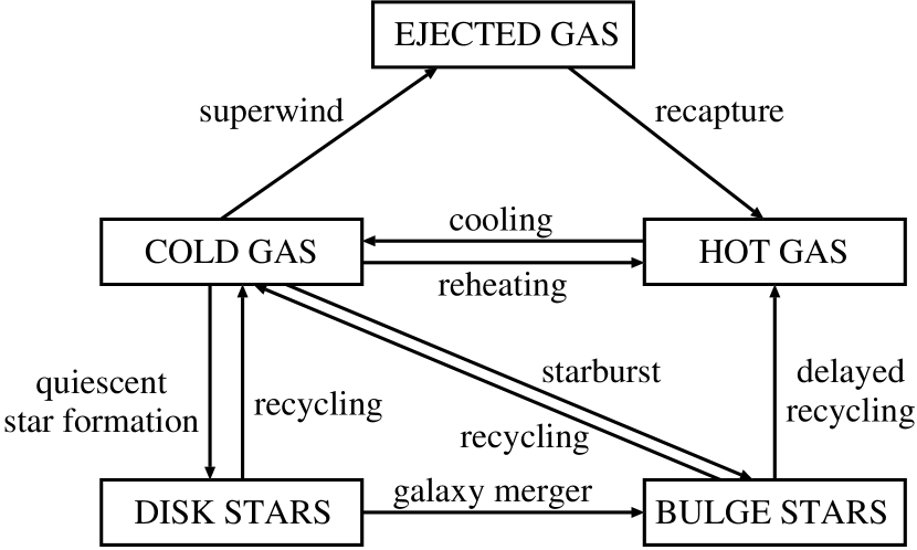
Figure 1: Diagram showing the different baryonic components included in the model, and the mechanisms by which mass and metals are exchanged between them.

3 STELLAR EVOLUTION AND METAL ENRICHMENT

Our galaxy formation model thus has baryons in four different components: stars in galaxies, cold gas in galaxies, hot gas in halos, and hot gas outside halos. There are exchanges of material between stars and cold gas, cold gas and hot gas inside halos, cold gas and hot gas outside halos, and hot gas outside and inside halos, as described in the previous section. In addition, mergers of halos mix their reservoirs of hot gas, and mergers of galaxies mix the stellar and cold gas components of the two galaxies. The exchanges of mass and metals between the different baryonic components are shown schematically in Fig. 1. Our model keeps track of the effects of all of these mass exchanges and merging events on the metallicities of the different components. Finally, we must calculate the production of new heavy elements inside stars and their ejection back into the gas phase. We describe now how we model this last process.

3.1 Evolution of a single stellar population

Stars lose mass through stellar winds as they evolve. Some stars ultimately undergo supernova explosions which pollute the interstellar medium with newly produced metals. The rates of both of these phenomena depend upon the mass of the star. The total amount of gas recycled and metals produced per unit stellar mass depends, therefore, on the adopted IMF. In this Section we explain how we obtain the gas restitution rate, the rates of SNe II and SNe Ia and the chemical yield for a single stellar population. This information is then incorporated directly into the galform model, which predicts the star formation histories of individual galaxies, in order to obtain these quantities for the model galaxies. The discussion below is based upon that given by Lia, Portinari & Carraro (2002) with slight differences. Stellar data are extracted from Portinari, Chiosi & Bressan (1998) for massive stars and Marigo (2001) for intermediate and low mass stars. The chemical yields of SNe Ia are taken from Nomoto et al. (1997).

Figure 2: The initial mass functions (IMFs) of star formation used in this paper, $\phi(m)\equiv{\rm d}N/{\rm d}\ln m$. For quiescent star formation we use the Kennicutt (1998) IMF (solid line) and for starbursts we use a flat IMF (dashed line). In both cases the IMFs are normalised to be unity when integrated over the whole range of mass.

We define the IMF as the number of stars per logarithmic interval of stellar mass per unit total mass of stars formed:

$$\phi(m)\equiv{\rm d}N/{\rm d}\ln m\propto m^{-x},$$ (9)

normalised to unity when integrated over the whole range of mass

$$\int_{m_{d}}^{m_{u}}m\,\phi(m)\,d\ln m=\int_{m_{d}}^{m_{u}}\phi(m)\,dm=1.$$ (10)

so that $\phi(m)$ has units of $M_{\odot}^{-1}$. In this paper, we use the IMF proposed by Kennicutt (1983) for quiescent star formation in disks, and a flat IMF in starbursts triggered by galaxy mergers. The Kennicutt (1983) IMF has $x=0.4$ for $m<1M_{\odot}$ and $x=1.5$ for $m\geq 1M_{\odot}$. In starbursts, $x=0$. In both modes of star formation, the lower and upper stellar mass limits of the IMF are $(m_{d},m_{u})=(0.15M_{\odot},120M_{\odot})$. Fig. 2 shows the quiescent (solid line) and starburst (dashed line) IMFs.

In addition to the visible stars with $m>0.15M_{\odot}$, we allow for brown dwarfs with $m<0.15M_{\odot}$. The mass fraction of brown dwarfs is quantified by $\Upsilon$, which is the ratio of the total mass in stars to the mass in visible stars for a newly formed population of stars. Thus, the mass fraction in visible stars is $1/\Upsilon$. CLBF adopted the Kennicutt IMF in both the quiescent and burst modes of star formation, and required $\Upsilon=1.38$ to match the predictions of their fiducial model to the observed present-day galaxy luminosity function around $L_{*}$. The other models we consider in this paper have $\Upsilon=1$.

The recycled mass fraction from an evolving population of stars is a function of time. For a population of stars formed with an IMF $\phi(m)$ at time $t=0$, the total mass fraction released by time $t$ is

$$E(\leq t)=\int_{M(t)}^{m_{u}}[m-M_{\rm r}(m)]\,\phi(m)\frac{dm}{m},$$ (11)

where $M(t)$ is the mass of a star reaching the end of its life at time $t$, and $M_{\rm r}(m)$ is the mass of the remnant left by a star with initial mass $m$. In our model, since the timestep we use is roughly comparable to the lifetime $4\times 10^{7}$yr of an 8$M_{\odot}$ star, the lowest mass star that results in a SNe II, we can justifiably use the instantaneous recycling approximation for SNe II. We therefore instantaneously release the mass recycled by stars with $M\geq 8M_{\odot}$. In Fig. 3, we show $E(\leq t)$ for both IMFs considered. The dotted lines show how these predictions change if the assumption of instantaneous recycling is relaxed.

Figure 3: The cumulative returned mass fraction, $E(\leq t)$, from evolved stars after time $t$ has elapsed from the epoch of star formation. The solid and dashed lines indicate the $E(\leq t)$ we use for the Kennicutt and top-heavy IMFs, respectively. Because we assume the instantaneous recycling for SNe II, the values are constant until $\tau(8M_{\odot})$, where $\tau(m)$ is the lifetime of a star of mass $m$. The dotted lines show how these results change when the instantaneous recycling approximation is dropped.

The cumulative number of SNe II explosions up to time $t$ (per $M_{\odot}$ of stars formed), $R_{\rm II}(\leq t)$, and the mass fraction of metals of the $i$-th element, $E_{i}(\leq t)$, released up to time $t$ are given respectively by

$$R_{\rm II}(\leq t) = \int_{\max\{M(t),8M_{\odot}\}}^{m_{u}}\phi(m)\frac{dm}{m},$$ (12)

$$E_{i}(\leq t) = \int_{M(t)}^{m_{u}}M_{i}(m)\phi(m)\frac{dm}{m},$$ (13)

where $M_{i}(m)$ is the mass of the $i$-th element released from a star with mass $m$. Because $E_{i}(\leq t)$ includes metals that already existed when the stars formed, these pre-existing metals must be subtracted in order to estimate the chemical yields, $p_{i}(\leq t)$. If the metallicity of stars with respect to the $i$-th element at their birth is $Z_{i}^{0}$, $E_{i}$ can be divided into two terms,

$$E_{i}(\leq t)=p_{i}(\leq t)+Z_{i}^{0}E(\leq t),$$ (14)

where

$$p_{i}(\leq t)=\int_{M(t)}^{m_{u}}y_{i}(m)\phi(m)\frac{dm}{m},$$ (15)

and $y_{i}(m)$ indicates the mass of newly produced $i$-th element in a star with mass $m$. Portinari et al. (1998) show that the dependence of $M_{i}$ and $y_{i}$ on initial stellar metallicity is small, so for simplicity we neglect this dependence and use the values for solar initial metallicity throughout.

In Figs. 4 and 5, we show $R_{\rm II}(\leq t)$ and $p_{i}(\leq t)$, respectively. In both cases, the solid and dashed lines denote the Kennicutt and top-heavy IMFs respectively. The initial time for which results are plotted corresponds to $\tau(m_{u})$ and the final time to $\tau(8M_{\odot})$, where $\tau(m)$ is the lifetime of a star of mass $m$. In Fig. 5, the lines indicate the yields of O, Si, Mg, Fe from top to bottom at the right hand side of the panel. In this paper, because instantaneous recycling is assumed for SNe II, we only use the values of chemical yields at $\tau(8M_{\odot})$.

Note that we rescale the Mg yields from SNe II, $p_{\rm Mg}$, upwards by a factor of 4, so that the Mg abundances predicted by the model are more consistent with observed abundances in solar neighbourhood stars. This correction is standard practice in chemical evolution modelling, and is justified because the theoretical calculations of the yield of Mg are known to have a large (factor $\sim 3$) uncertainty (Timmes, Woosley & Weaver, 1995; Thomas, Greggio & Bender, 1998; Portinari, Chiosi & Bressan, 1998; Lia, Portinari & Carraro, 2002). In reality, any correction to the yields $y_{Mg}(m)$ is likely to depend on stellar mass, so the correction factor for the integrated yield $p_{\rm Mg}$ could be different for the two IMFs we use. In our model, the enrichment of galactic disks is dominated by stars formed with the Kennicutt IMF, while the $\alpha$-element enrichment of the ICM is predicted to be dominated by stars formed with the top-heavy IMF, and in fact, comparison with solar neighbourhood abundances favours a lower correction factor ($\sim$2-3) for the Mg yield than do the ICM abundances. However, for simplicity we have assumed the same correction factor for both IMFs.

Figure 4: The cumulative SNe II rate. The lines types are the same as in Fig. 2.

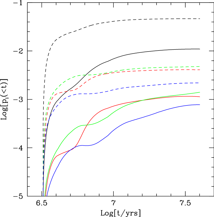
Figure 5: The cumulative chemical yields of SNe II, $p_{i}(\leq t)$. The solid and dashed lines denote the Kennicutt and top-heavy IMFs respectively. For each case, the lines indicate O, Si, Mg and Fe in sequence from top to bottom at $t=\tau(8M_{\odot})=4\times 10^{7}$yr.

The standard scenario (Whelan & Iben, 1973) for SNe Ia is that they occur in binary systems, in which a C-O white dwarf produced by evolution of the primary star accretes gas from the secondary star when the secondary overflows its Roche lobe at the end of its own evolution. This gas accretion drives the mass of the primary white dwarf over the Chandrasekhar limit, causing it to explode. We model this using the scheme of Greggio & Renzini (1983), with parameters updated according to Portinari, Chiosi & Bressan (1998). The progenitors of SNe Ia are assumed to be binary systems with initial masses in the range $m_{B,\rm low}<m_{B}<m_{B,\rm up}$, where $m_{B}\equiv m_{1}+m_{2}$, and $m_{1}$ and $m_{2}$ are the initial masses of the primary and secondary ($m_{2}\leq m_{1}$) respectively. We assume $m_{B,\rm up}=2m_{1,\rm max}$, where $m_{1,\rm max}$ is the largest single-star mass for which the endpoint is a C-O white dwarf. The binary star systems which are the progenitors of SNe Ia are assumed to have an initial mass function $A\phi(m_{B})$, where $\phi(m)$ is the same as for the single-star IMF. The distribution of mass fractions for the secondary, $\mu=m_{2}/m_{B}$, is assumed to have the form (normalised over the range $0<\mu<1/2$)

$$f(\mu)=2^{1+\gamma}(1+\gamma)\mu^{\gamma}\qquad\qquad(0<\mu<1/2).$$ (16)

For a single generation of stars formed at $t=0$, the cumulative number of SNe Ia explosions up to time $t$ is then given by

$$R_{\rm Ia}(\leq t)=A\int_{m_{B,\rm low}}^{m_{B,\rm up}}\phi(m_{B})\left[\int_{\mu_{\rm min}(t)}^{1/2}f(\mu)d\mu\right]\frac{dm_{B}}{m_{B}},$$ (17)

where the lower limit

$$\mu_{\rm min}(t)=\max\left[\frac{M(t)}{m_{B}},\frac{m_{B}-m_{B,{\rm up}}/2}{m_{B}}\right].$$ (18)

is set by the conditions that the secondary has evolved off the main sequence and that $m_{1}=m_{B}-m_{2}\leq m_{1,\rm max}$. Following Portinari et al. (1998), we adopt $m_{B,\rm low}=3M_{\odot}$, $m_{B,\rm up}=12M_{\odot}$ and $\gamma=2$. The factor $A$ is usually chosen (for given $m_{B,\rm low}$ and $\gamma$) to reproduce the observed ratio of rates of SNe Ia to SNe II in spiral galaxies. Following Portinari et al., we adopt $A=0.07$. This observational normalisation is derived for an IMF similar to Kennicutt, but for simplicity we assume that the same normalisation applies to the top-heavy IMF also.

In Fig. 6, we show the cumulative number of SNe Ia as a function of time, $R_{\rm Ia}(\leq t)$, for the Kennicutt IMF (solid line) and the top-heavy IMF (dashed line). The number of intermediate mass stars responsible for SNe Ia is larger in the case of the Kennicutt IMF than for the top-heavy IMF (as shown by Fig. 2). This is in contrast to the situation for SNe II. The yield of metals from SNe Ia is computed as

$$p_{{\rm Ia},i}(\leq t)=M^{\rm Ia}_{i}R_{\rm Ia}(\leq t),$$ (19)

where $M_{i}^{\rm Ia}$ is taken from the W7 model of Nomoto et al. (1997) and takes the values of 0.143, 8.5$\times 10^{-3}$, 0.154 and 0.626 $M_{\odot}$ for O, Mg, Si and Fe respectively.

Figure 6: The cumulative SNe Ia rate, $R_{\rm Ia}$. The line types are the same as those used in Fig. 2. Note that the SNe Ia rate for the top-heavy IMF is smaller than that for the Kennicutt IMF, because the top-heavy IMF has fewer intermediate mass stars.

Note that if the IMF includes a fraction of brown dwarfs (with $\Upsilon>1$), the values in equations (11), (12), (15), (17) and (19) must be multiplied by $1/\Upsilon$, because $\Upsilon>1$ corresponds to having a fraction $1/\Upsilon$ of visible stars with $m_{d}<m<m_{u}$.

3.2 The metal enrichment of cold and hot gas

We treat the metal enrichment due to SNe II in the same way as CLBF, except that the instantaneously returned mass fraction and yields (denoted $R$ and $p$ in CLBF) are replaced here by $E(\leq\tau[8M_{\odot}])$ and $p_{i}(\leq\tau[8M_{\odot}])$. The mass released from evolved stars after $\tau(8M_{\odot})$ and the metals produced by SNe Ia are computed at every timestep. The gas and metals recycled from disk stars are put into the cold gas in the galaxy, while those from bulge stars are put into the hot gas in the halo. This picture is consistent with many evolutionary models of disk galaxies, in which metals from SNe Ia are put into the gaseous disk; observations suggest that elliptical galaxies do not keep the metals released from SNe Ia, because the metal abundances in the interstellar medium of ellipticals are either smaller than or at best similar to solar abundances (Matsushita, Ohashi & Makishima, 2000).

The mass released from stars during the time interval $t_{i}<t<t_{i+1}$ is computed from

$$\Delta M=\int_{0}^{t_{i+1}}[E(\leq t_{i+1}-t^{\prime})-E(\leq t_{i}-t^{\prime})]\psi(t^{\prime})dt^{\prime},$$ (20)

where $\psi(t)$ is the star formation rate at time $t$ for the galaxy under consideration. In order to solve this equation, the star formation histories in both modes of star formation, quiescent and starburst, must be recorded separately for individual galaxies. Due to the memory overhead involved, the star formation histories are rebinned into 30 linear steps in time. We have confirmed that our results are insensitive to the precise number of steps used.

As well as the returned mass, the metals produced by evolving stars, including SNe Ia, are computed in a similar way. The mass of the $i^{\rm th}$ element released from evolved stars and SNe Ia over the time interval [$t_{i},t_{i+1}$] is

$$\Delta M_{i}=\int_{0}^{t_{i+1}}M_{i}^{Ia}[R_{\rm Ia}(\leq t_{i+1}-t^{\prime})-R_{\rm Ia}(\leq t_{i}-t^{\prime})]\psi(t^{\prime})dt^{\prime}$$

$$+\int_{0}^{t_{i+1}}Z(t^{\prime})[E(\leq t_{i+1}-t^{\prime})-E(\leq t_{i}-t^{\prime})]\psi(t^{\prime})dt^{\prime},$$ (21)

where $Z(t)$ is the metallicity of stars at their birth at time, $t$; this quantity is stored in the same fashion as the star formation histories. The metals are also assumed to be put into cold and hot phases along with the recycled gas.

4 The galaxy luminosity function

In this paper we consider three principal models: the fiducial model of CLBF (which assumed $\Omega_{b}=0.02$) and two new models which have $\Omega_{b}=0.04$. The first of these new models is superwind model, in which gas ejection from the halo is invoked to suppress the formation of bright galaxies. In the second new model, which we refer to as the conduction model, cooling in massive halos is suppressed by thermal conduction. In the CLBF model, all stars form with a Kennicutt IMF. In the superwind and conduction models, the Kennicutt IMF is adopted for quiescent star formation in disks and a flat IMF is used in starbursts. The superwind model is similar to the model used by Baugh et al. (2004b). We also consider a variant of the superwind model (which we denote superwind/Kennicutt) in which all star formation produces stars with a Kennicutt IMF. We list the parameters for the different models in Table 1.

Table 1: Model parameters. Column 1 gives the name of the model, column 2 gives the baryon density parameter, column 3 gives $\Gamma$, the CDM power spectrum shape parameter. Column 4 gives the dark matter halo mass function used; J and PS denote mass functions given by Jenkins et al. (2001) and Press & Schechter (1974) respectively. Columns 5 and 6 give the parameters that specify the quiescent star formation timescale, as defined by eqn. (1). Note that in the CLBF model, the star formation timescale scales with the dynamical time of the disk, $\tau_{\rm disk}$. Column 7 gives the value of the $V_{\rm hot}$ parameter that determines the strength of the standard SNe feedback (eqn. 3). Columns 8 and 9 describe the superwind feedback; column 8 gives the parameter that sets the strength of the superwind (eqn. 8) and column 9 gives the threshold circular velocity of halos above which gas ejected by a superwind can be recaptured. Column 10 gives the circular velocity of halos above which cooling is suppressed in the conduction model. Column 11 gives the IMF assumed in bursts; note that all models assume a Kennicutt IMF for quiescent star formation. Finally, column 12 gives the ratio of total stellar mass to the mass produced in luminous stars.

(1)	(2)	(3)	(4)	(5)	(6)	(7)	(8)	(9)	(10)	(11)	(12)
model	$\Omega_{\rm b}$	$\Gamma$	MF	$\tau_{*}^{0}$ (Gyr)	$\alpha_{*}$	$V_{\rm hot}({\rm kms}^{-1})$	$f_{\rm SW}$	$V_{\rm recap}$ (km s-1)	$V_{\rm cond}^{0}$ (km s-1)	burst IMF	$\Upsilon$
superwind	0.04	0.172	J	8	-3	200	2	600	–	x=0	1
superwind/	0.04	0.172	J	8	-3	200	2	600	–	Kenn	1
Kennicutt
conduction	0.04	0.172	J	8	-3	300	0	–	100	x=0	1
CLBF	0.02	0.19	PS	200$\tau_{\rm disk}$	-1.5	200	0	–	–	Kenn	1.38

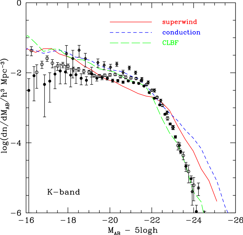
Figure 7: The K-band galaxy luminosity function at $z=0$. The model predictions are shown by the lines as indicated by the key. The symbols with error bars show observational data from Cole et al. (2001, filled circles), Huang et al. (2003, stars), and Bell et al. (2003, open circles).

An important constraint on the models is that they should be consistent with the observed present-day galaxy luminosity function. In Fig. 7 we compare the model predictions for the present-day $K$-band luminosity function with observational estimates. The predictions of the superwind model with $V_{\rm recap}=600$ km s^-1 are shown by the solid line, those of the conduction model with $V_{\rm cond}^{0}=100$ km s^-1 by the short dashed line, and the luminosity function of the CLBF model is plotted using a long dashed line. The symbols show observational data. Although it is challenging for models with the currently favoured value of $\Omega_{\rm b}$ to match the observed luminosity function as well as in the CLBF model, as shown by Benson et al. (2003a), the superwind and conduction models are in broad agreement with the observations.

In the conduction model, the value of the parameter $V_{\rm cond}^{0}$ which is required to produce a good match with the observed luminosity function seems unphysically small. The value of $V_{\rm cond}^{0}=100{\rm kms}^{-1}$ requires a thermal conductivity that is many times larger than the Spitzer value. As explained in Section 2, processes other than thermal conduction could also contribute to the suppression of cooling, so we retain the freedom to adopt such a low value for this parameter.

In Fig. 8 we show how the luminosity function in the superwind model depends on the parameter $V_{\rm recap}$, the threshold circular velocity above which halos recapture gas previously ejected in a superwind. Clearly if $V_{\rm recap}$ is too low, then too many very bright galaxies are produced. On the other hand, the galaxy luminosity function becomes insensitive to increases of this parameter above $V_{\rm recap}\approx 600$ km s^-1. However, as we will show later, the value of $V_{\rm recap}$ has a strong impact on metal abundances in the ICM. The predicted ICM metal abundances are too low unless the metals ejected in the superwind can be recaptured by cluster-sized halos. Thus, we require a value $V_{\rm recap}\simeq 600$ km s^-1 in order to reproduce both the observed field galaxy luminosity function and the metal abundance of the ICM.

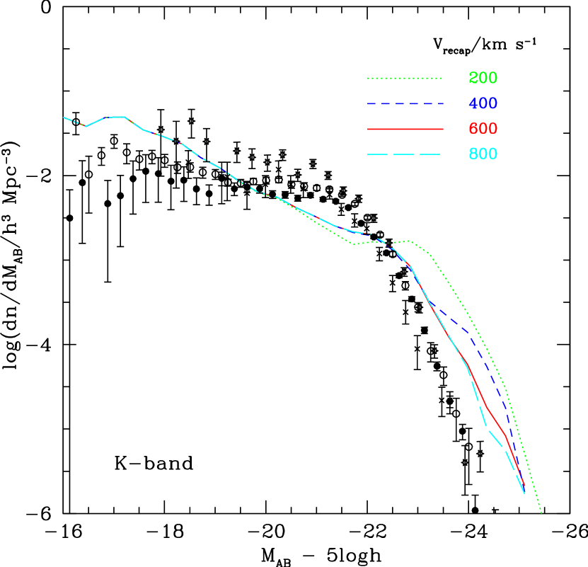
Figure 8: The K-band luminosity function predicted in the superwind model for different values of $V_{\rm recap}$, the threshold halo circular velocity for the recapture of gas previously ejected by a superwind (as indicated by the key). The fiducial superwind model has $V_{\rm recap}=600{\rm kms}^{-1}$ and is shown by the solid line. The observational data are plotted using the same symbols as in Fig. 7.

5 Present-day intracluster medium

5.1 Gas mass-to-stellar luminosity ratio and hot gas fraction

A basic test for any model of the chemical enrichment of the ICM is that it should reproduce the observed ratios of the ICM mass to total stellar luminosity and to total mass in clusters. This is because the metals are produced in stars, so a model which produces the observed ICM metallicity is invalid unless it predicts the correct number of stars at the same time.

In Fig. 9, we plot the ratio $M_{\rm hot}/L_{b_{\rm J}}$ of the mass of the ICM, $M_{\rm hot}$, to the total $b_{\rm J}$-band stellar luminosity of the galaxies, $L_{b_{\rm J}}$, as a function of the ICM temperature $T$. We show predictions for the superwind, conduction and CLBF models. In the models, the ICM temperature is assumed to equal the halo virial temperature,

$$T_{vir}=\frac{1}{2}\frac{\mu m_{H}}{k_{B}}V_{c}^{2}=3.1{\rm keV}\left(\frac{V_{c}}{1000{\rm kms}^{-1}}\right)^{2},$$ (22)

while for the observations we use the measured X-ray temperature. The relationship between cluster mass and virial temperature in the $\Lambda$CDM model at $z=0$ is then $T_{vir}=6.4{\rm keV}\,(M/10^{15}h^{-1}M_{\odot})^{2/3}$. We compare the models with observational data from Sanderson et al. (2003) and Sanderson & Ponman (2003). We have combined the data from individual clusters in bins in X-ray temperature, and computed the mean and dispersion in each bin, weighted according to the errors on the individual datapoints. The error bars on the plotted datapoints are calculated from the dispersion in each bin, and do not include any other measurement errors.

The conduction and CLBF models predict a ratio $M_{\rm hot}/L_{b_{\rm J}}$ which increases only slightly with cluster temperature. The superwind model predicts a somewhat larger increase, because of the expulsion of gas from lower-mass halos, but again is almost flat for halos with $V_{c}>V_{\rm recap}$, corresponding to $T\approx 1.1$keV which is indicated by the vertical dashed line in the top panel. The models are in approximate agreement with the observational data for $T\gtrsim 2$keV, but for lower temperatures, the observations suggest ICM fractions significantly smaller than what the models predict. However, there are still important uncertainties in the observational data (not included in the error bars plotted) resulting from the need to extrapolate X-ray measurements out to the cluster virial radius, so the ICM fractions in cooler clusters are not yet securely determined as shown below.

We note that the CLBF model predicts very similar $M_{\rm hot}/L_{b_{\rm J}}$ values to the superwind and conduction models, even though it has a global baryon fraction only half that of the other models. This agreement comes about because the CLBF model predicts a luminosity density which is a factor $\sim 2$ lower in all environments compared to the other models.

In Fig. 10 we show the ratio of the ICM mass to the total cluster mass including dark matter as a function of cluster temperature. The dots and crosses indicate the hot gas fractions for the superwind and the conduction models, respectively. The dashed horizontal line corresponds to the cosmic baryon-to-total mass ratio; the model points would all lie on this line if all baryons were retained in the cluster in the hot gas component. We also show observational data from Sanderson et al. (2003), binned in temperature as in Fig. 9. The superwind model reproduces the qualitative trend seen in the observations that the gas fraction drops in low temperature clusters. However, we caution that the observational estimates rely on extrapolating both the ICM and dynamical masses from the outermost measured X-ray datapoint out to the halo virial radius. Future more accurate X-ray observations will allow more precise tests of models for gas ejection from halos.

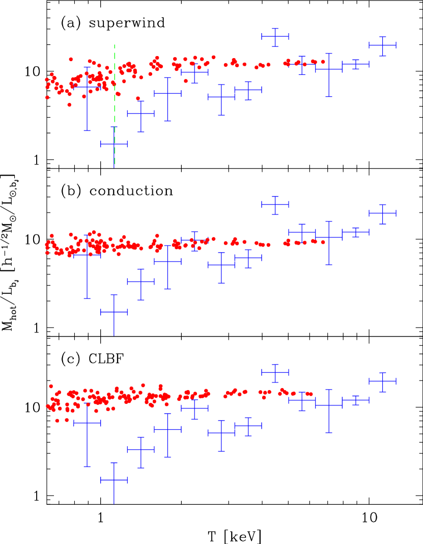
Figure 9: The ratio of ICM mass to $b_{\rm J}$-band luminosity of stars contained in a cluster, $M_{\rm hot}/L_{b_{\rm J}}$, plotted as function of the hot gas temperature. The dots show the predictions of: (a) the superwind model, (b) the conduction model, and (c) the CLBF model. The crosses in all panels denote the binned averages of $M_{\rm hot}/L_{b_{\rm J}}$ estimated using observational data from Sanderson et al. (2003) and Sanderson & Ponman (2003). The dashed vertical line in panel (a) shows the temperature corresponding to a halo circular velocity $V_{\rm recap}=600$ km s^-1, above which ejected gas is recaptured.

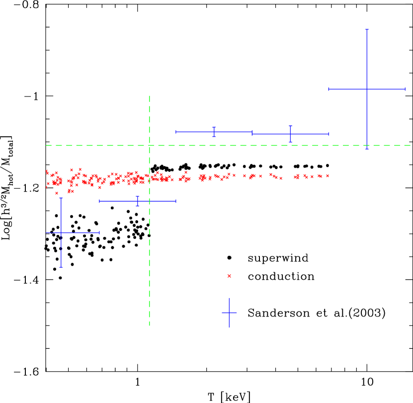
Figure 10: The ratio of hot gas mass to total mass, including dark matter, as a function of the hot gas temperature. The dots and crosses show the predictions of the superwind model and the conduction model, respectively. The points with error bars show the binned averages of the observational data from Sanderson et al. (2003) (we use their estimates of gas fraction wihthin the virial radius). The horizontal dashed line indicates the universal ratio of baryon to total mass density estimated from $\Omega_{0}$ and $\Omega_{\rm b}$. The vertical dashed line shows the temperature corresponding to a halo circular velocity $V_{\rm recap}=600$ km s^-1, above which ejected gas in the superwind model is recaptured.

5.2 Metal abundances

We now compare the ICM metallicities predicted by our models with observational data. Our model predicts global metallicities, averaged over the entire ICM within the cluster virial radius. In contrast, the ICM metallicities measured from X-ray data are often only representative of the central regions of the cluster, because these dominate the X-ray emission. Some clusters, known as cooling flow clusters, show metallicity gradients for some elements, in the sense that metallicities increase towards the cluster centre. It is therefore essential to correct the observational data to estimate mean metallicities averaged over the entire cluster, before comparing with the models. We compare our model predictions with the following observational data on ICM abundances: De Grandi et al. (2004, BeppoSAX) for Fe [see also Irwin & Bregman (2001) and De Grandi & Molendi (2002)]; Peterson et al. (2003, XMM-Newton) for O, Fe, Mg and Si [see also Tamura et al. (2004)]; Fukazawa et al. (1998, ASCA) for Fe and Si; and Baumgartner et al. (2003, ASCA) for Si. We explain in the Appendix why we have omitted some observational data from our comparison. We use the results of the systematic study of iron gradients by De Grandi et al. (2004) to convert the measured central metallicities of iron and silicon to global average values, assuming that silicon has the same gradient as iron, as is suggested by observational data. We present the details of how we make these corrections in the Appendix. The size of these estimated corrections is up to a factor of two. Oxygen and magnesium do not show metallicity gradients (Tamura et al., 2001, 2004), so we assume that the global abundances of these elements are equal to the measured central values. We note that previous studies (e.g. de Lucia et al. 2004) have not included any correction for metallicity gradients when comparing models with observed ICM abundances.

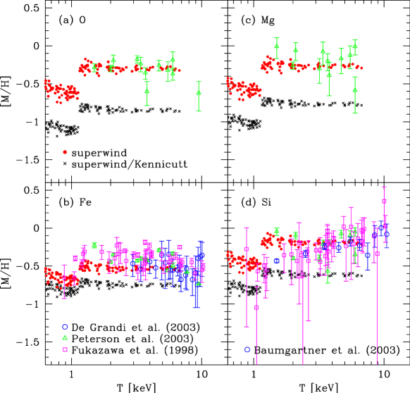
Figure 11: The metal abundances of the ICM. Each panel shows a different element: (a) [O/H] (b) [Fe/H] (c) [Mg/H] (d) [Si/H]. Abundances are normalized to solar values, and shown on a logarithmic scale. The predictions of the superwind model are shown by dots in the standard case where starbursts have a top-heavy IMF, and by crosses for the variant model in which all star formation takes place with a Kennicutt IMF. The open triangles in each panel denote observational data from XMM-Newton (Peterson et al., 2003), and the open squares data from ASCA (Fukazawa et al., 1998); in panel (b), the open circles show data from BeppoSAX (De Grandi et al., 2004), while in panel (d), the open circles show ASCA data from Baumgartner et al. (2003). All of the datapoints are measurements for individual clusters, apart from Baumgartner et al. (2003), which are average values in bins of temperature. The observational data have been corrected for abundance gradients as described in the text.

We first show how the predicted metal abundances in the ICM depend on the IMF adopted for starbursts. Fig. 11 shows the O, Fe, Mg and Si abundances (relative to solar values) as functions of cluster temperature for the superwind model. The dots show the predicted values for the standard superwind model with a top-heavy IMF ($x=0$) in bursts and a Kennicutt IMF in disks, and the crosses show a variant superwind model in which disks and bursts both have a Kennicutt IMF. For clusters with $T\gtrsim 1$keV, the abundances of the $\alpha$-elements O, Mg and Si are 3–4 times higher in the case of the top-heavy IMF in bursts, while the abundance of Fe is only about 60% higher. This difference reflects that fact that the $\alpha$-elements are produced mostly by SNe II, and the number of SNe II is larger for a top-heavy IMF, while Fe is produced by both SNe Ia and SNe II, and the number of SNe Ia is actually reduced for the top-heavy IMF. In fact, the models predict that most Fe is produced by SNe Ia for a Kennicutt IMF, but by SNe II for the top-heavy IMF.

When in Fig. 11 we examine the dependence of ICM abundances on cluster temperature (or mass) in the superwind model, we see that the abundances of the different elements all show a break at $T\approx 1.1$ keV. This temperature corresponds exactly to the halo circular velocity $V_{\rm recap}=600$ km s^-1 above which gas and metals ejected by superwinds are recaptured. Halos with $V_{c}>V_{\rm recap}$ effectively trap all of the metals ever produced by the galaxies they contain. For clusters hotter than the break, the abundances are predicted to be almost constant. The jump in abundances across the break is about a factor 2 for O, Mg and Si, but is much smaller for Fe, especially if a Kennicutt IMF is used in bursts. This again reflects the fractions of these different elements produced in either SNe II or SNe Ia. Since SNe II also drive the superwinds, while SNe Ia are typically delayed until after the strong superwind phase has subsided, superwinds are much more effective in expelling from halos the heavy elements produced in SNe II than those produced in SNe Ia. If $V_{\rm recap}$ is varied, then the metal abundances in clusters with $V_{c}>V_{\rm recap}$ are insensitive to the value of $V_{\rm recap}$ for $V_{\rm recap}\ga 400$ km s^-1, but increase slightly if $V_{\rm recap}\la 400$ km s^-1, because more stars are produced in that case (c.f. Fig.8).

Fig. 11 also shows the observed ICM abundances of O, Mg, Si and Fe, corrected to global average values as we have described. We see that the superwind model with a top-heavy IMF in bursts agrees well with the observed abundances of O, Mg and Si, while the superwind model with a Kennicutt IMF predicts abundances of these elements which are too low by factors 2–3. For Fe, the model with the top-heavy IMF again agrees better with the observations, although the abundance is still slightly low. We note that the current abundance measurements for O, Mg and Si are all for clusters hotter than the break predicted in the models. However, the value of $V_{\rm recap}$ cannot be significantly increased above our standard value of 600 km s^-1 without moving the abundance break into the temperature range where the observations indicate a plateau in abundances, thus conflicting with the data. The measured Fe abundances, which extend down to somewhat lower cluster temperatures, do in fact suggest a break close to the temperature predicted by the superwind model, but more measurements for cool ($T<1$keV) clusters are needed to confirm this. It is clear that more abundance measurements in cool clusters, especially of O, Mg and Si, would put stringent constraints on our model of ejection of gas and metals from halos by superwinds. The models also predict a very small scatter in global ICM abundances at a given cluster temperature, especially above the break. The observed abundances show a larger scatter, but most of this results from measurement errors.

In Fig. 12 we show the ICM metal abundances predicted by our other two models: the conduction model with a top-heavy IMF in bursts, and the CLBF model with a Kennicutt IMF for all modes of star formation. The models are compared with the same observational data as in Fig. 11. For both of these models, halos retain all of their metals, and consequently the predicted ICM abundances are almost constant with cluster temperature. The CLBF model predicts abundances too low compared to observed values, by factors 2–3 for O, Mg and Si, and by around 40% for Fe, and is thus ruled out. The conduction model predicts abundances in much better agreement with observations, although slightly too high for O and Si. The abundances in the conduction model are slightly higher overall than those in the superwind model.

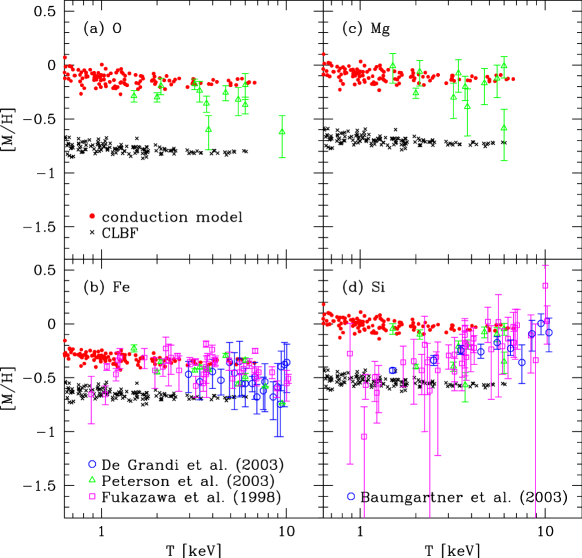
Figure 12: The metal abundances in the ICM for the conduction model (dots) and the CLBF model (crosses). The observational data are plotted using the same symbols as in Fig. 11.

It should be remembered that we have applied a correction to the yield of Mg from SNe II predicted by stellar models, in order to better match observational constraints. The model yields have been multiplied by a factor of four throughout, a value which is a compromise between that required to reproduce Mg abundances in galactic disks (specifically, in the solar neighbourhood) and in the ICM; a separate correction factor could be applied to each IMF because of the mass-dependent uncertainties in estimating theoretical yields. No correction factors have been applied to the yields of the other elements: O, Fe and Si.

5.3 Abundance ratios

Examining the abundance ratios between different elements in the ICM provides an alternative method to constrain the form of the IMF, in which the effects of uncertainties in the ICM to stellar mass ratio cancel out. In Fig. 13 we show the abundance ratios of different $\alpha$ elements to iron, [O/Fe], [Mg/Fe] and [Si/Fe], for the standard superwind model, with a top-heavy IMF in bursts, and the variant superwind model, with a Kennicutt IMF in bursts. We also show observational data from Peterson et al. (2003), which in the case of Si and Fe have been corrected for abundance gradients in the way already described. We see that the predicted O/Fe and Mg/Fe ratios agree better with observations for the model with the top-heavy IMF, while on the other hand the Si/Fe ratio agrees better with the model having a Kennicutt IMF in bursts. The overall level of agreement of the abundance ratios with observational data in the top-heavy IMF model could be improved if the Fe abundances in the model were slightly larger (this can also be seen in Fig. 11), or if the observed Si abundances were slightly larger. The latter would occur if the abundance gradients in Si were weaker than we have assumed, since we would then infer larger global Si abundances from the same measured central values. However, recent data from Tamura et al. (2004), in which metal abundances are measured out to $r\la 500h^{-1}$ kpc from cluster centres, seem to support our original assumption that the radial gradients in Si and Fe are the same.

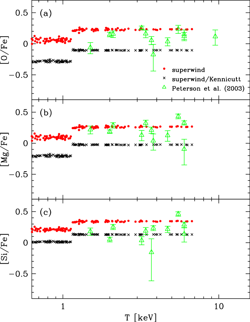
Figure 13: The abundance ratios of $\alpha$-elements to iron. Each panel corresponds to a different ratio: (a) [O/Fe]. (b) [Mg/Fe]. (c) [Si/Fe]. All ratios are relative to solar values. The predictions of the superwind model are plotted using dots for the standard case in which starbursts have a top-heavy IMF, and crosses when all star formation is with the Kennicutt IMF. The open triangles show observational data from Peterson et al. (2003), corrected for radial gradients.

Fig. 14 is the equivalent of Fig 13 for the conduction and CLBF models. Since the conduction model predicts slightly higher Fe abundances than the superwind model, the agreement with the observed abundance ratios improves. The CLBF model fails to reproduce the observed abundance ratios. The models predict very little variation in the abundance ratios with cluster temperature, apart from the break in the superwind model where recapture sets in. They also predict very small scatter for the abundance ratios at a given cluster temperature.

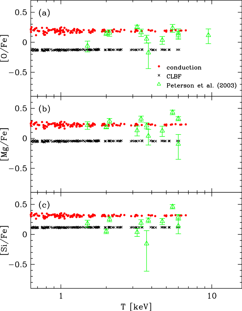
Figure 14: The abundance ratios in the conduction model (dots) and the CLBF model (crosses). The data are the same as plotted in Fig. 13.

5.4 Metallicities of stars and gas in clusters

In Fig. 15 we compare the predicted mass-weighted mean iron metallicities for the different baryonic components in clusters: stars in galaxies, cold gas in galaxies, and hot intracluster gas. Results are shown for the standard superwind and conduction models as functions of cluster temperature. In both models, the mean stellar and cold gas metallicities are close to solar, while the hot gas metallicity is 2–3 times lower. The mean total metallicity is only slightly larger than the hot gas metallicity, reflecting the fact that most of the baryons are in the hot gas component. For the superwind model, the onset of recapture of gas by halos produces the expected jump in the hot gas and total metallicities, but does not produce any corresponding feature in the metallicities of the stars or cold gas. This is because the enrichment of these components has almost finished by the formation epoch of the cluster and the epoch of recapture of expelled metals (see Section 7).

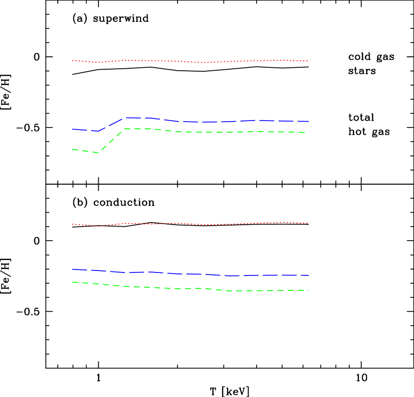
Figure 15: The iron metallicities, [Fe/H], of stars, cold gas and hot gas, shown by the solid, dotted and short-dashed lines, respectively. The mass-weighted, mean total metallicities are shown by the long-dashed line. Panel (a) shows results for the superwind model and (b) for the conduction model.

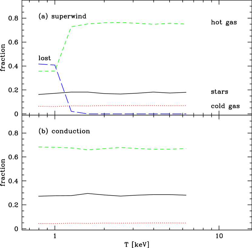
Figure 16: The mass fractions of iron in different components. The line types are the same as in Fig. 15 except for the long-dashed line, which indicate the fraction of iron in gas expelled from halos (labelled as ‘lost’).

Fig. 16 shows the fractions of the total mass of iron which are in stars, cold gas, hot gas and ‘lost’ gas which is expelled from halos by superwinds, for the same models as in Fig. 15. In all cases, more of the iron is in the hot gas than in galaxies. In the superwind model, superwinds put about 40% of the iron outside halos for low mass clusters below the threshold for recapture. Thus, according to this model, a significant mass of metals should be observed in the surroundings of low temperature clusters.

Thus, in summary, from the ICM results at $z=0$, we conclude that a top-heavy IMF with $x\simeq 0$ in starbursts is required for the model predictions to match the observed ICM metallicities, as long as we adopt the Kennicutt or a similar IMF for disk star formation. The use of a Kennicutt or a similar IMF for disk star formation is supported by many observations and models of solar neighbourhood stars, including a semi-analytic model by Nagashima & Okamoto (2004) in which a Salpeter-like IMF provides good agreement with the observed metallicities of solar-neighbourhood stars. We have also confirmed that while using the Arimoto-Yoshii IMF (Arimoto & Yoshii, 1987) with $x=1$ for both star formation modes substantially increases metallicities compared with the Kennicutt IMF, a combination of the Kennicutt IMF for quiescent star formation and the Arimoto-Yoshii IMF for starbursts does not reach the observed metallicities.

6 ICM ABUNDANCES IN HIGH-REDSHIFT CLUSTERS

6.1 Evolution of [Fe/H]

With the advent of the new generation of $X$-ray satellites, measurements of ICM metallicities are now becoming possible in high-redshift clusters, thus allowing direct tests of ICM evolution. In Fig. 17, we show what our models predict for the evolution of the iron abundance in the ICM with redshift in the range $0<z<1.3$. At each redshift, we calculate the mean Fe abundance for clusters in two different ranges of temperature, $3<T<5$keV and $5<T<8.5$keV. We show results for the standard conduction and superwind models. In the same figure we also show observational data from Tozzi et al. (2003), based on measurements of the iron abundances in 18 distant clusters with $0.3\la z\la 1.3$ using Chandra and XMM-Newton. We have binned this data in redshift and in the same ranges of temperature as used for the models. Note that we have no information about metallicity gradients for these distant clusters, so we have not applied any corrections to the measured abundances to get global values. We also show observational data for $z=0$ clusters binned in the same ranges of temperature. The $z=0$ data are corrected for metallicity gradients as previously described.

Our models predict a weak decline in the Fe abundance with increasing redshift, by about 30% over the range $0<z<1.3$, and furthermore this decline is predicted to be the same for both low and high temperature clusters. Tozzi et al. (2003) concluded from their own data that the evolution in Fe abundance with redshift is negligible, but we see that the data for the hotter ($5<T<8.5$keV) clusters are also quite consistent with the weak decline predicted by our models. The data for the cooler ($3<T<5$keV) clusters suggest higher Fe abundances and a weak increase with redshift relative to the hotter clusters, both of which would conflict with our model, but the uncertainties are very large.

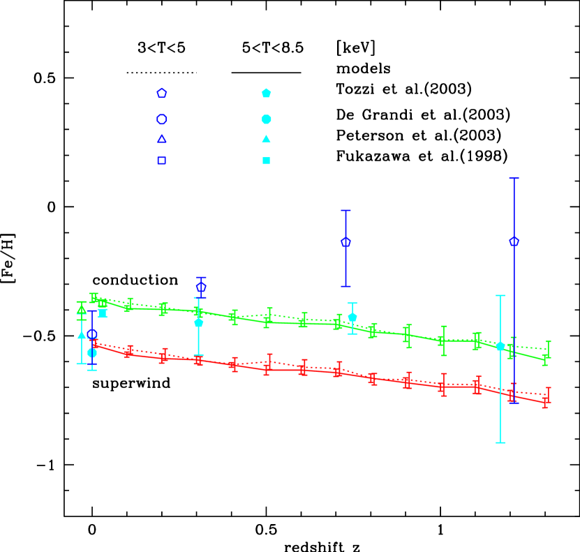
Figure 17: The redshift evolution of [Fe/H] in the ICM. The lines show the mean abundances predicted by the models for two different temperature ranges, 3-5keV (dotted) and 5-8.5keV (solid), for both the superwind and conduction models (lower and upper pairs of lines, as labelled). The error bars on the lines show the 1$\sigma$ scatter. The symbols show the observal data, with means and 1$\sigma$ scatter computed in each bin. Pentagons indicate the data for high redshift clusters from Tozzi et al. (2003), circles, triangles and squares are mean metallicities of clusters at $z=0$ given by De Grandi et al. (2004), Peterson et al. (2003) and Fukazawa et al. (1998), respectively. The symbols for $z=0$ are given small offsets for clarity. The observational data are binned into the same temperature ranges as the models.

6.2 Evolution of [O/Fe]

The abundances of elements other than Fe have not yet been measured in high-redshift clusters, so we simply present predictions for the evolution of O abundances from our model. For clusters selected in the same temperature range at different redshifts, the mean O abundance is predicted to decline with redshift even more weakly than for Fe, by only $\sim 10\%$ in over the range $0<z<1.3$. The difference in behaviour is caused by the difference in the timescales for enrichment by SNe Ia and SNe II. The O/Fe ratio in the ICM is therefore predicted to increase with redshift. This is shown in Fig. 18. For the superwind model, there is a significant difference in O/Fe between low (0.7-1 keV) and high (3-8.5 keV) temperature clusters, caused by recapture of superwind ejecta in clusters with $T\gtrsim 1.1$keV.

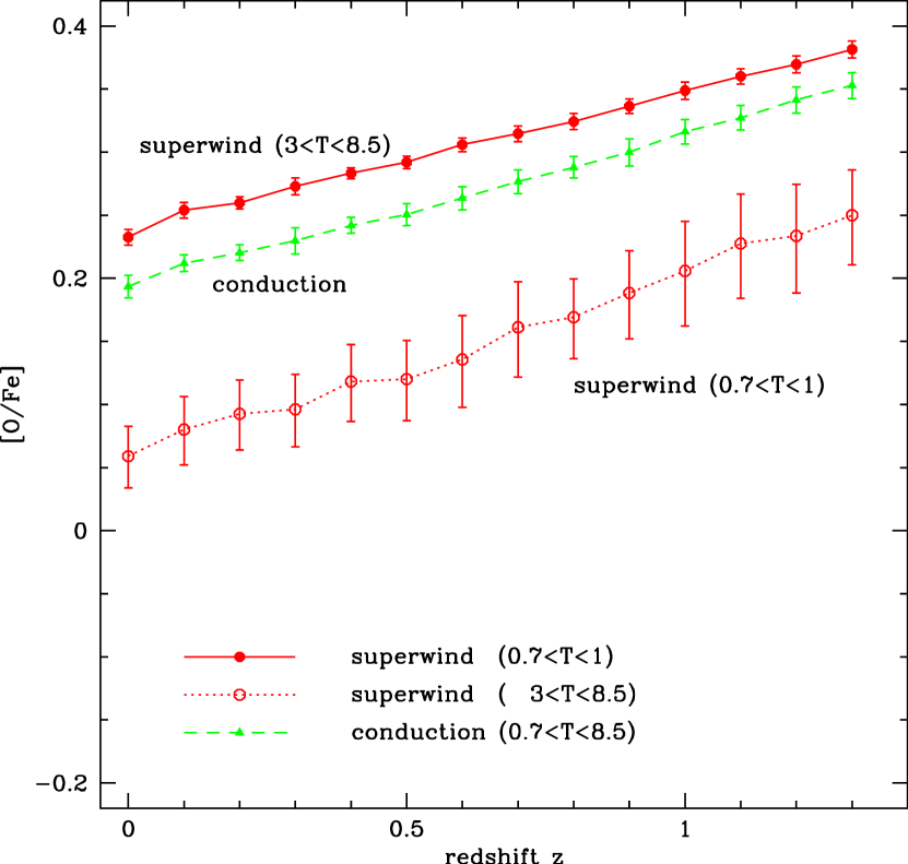
Figure 18: The redshift evolution of [O/Fe] in the ICM. The lines show the predictions for the conduction and superwind models respectively. In the case of the superwind model, the sample is divided into two temperature ranges: high (3-8.5 keV; solid line) and low (0.7-1 keV; dotted line) temperatures.

Figure 19: The evolution of the main progenitors of present-day clusters, as defined in the text. The left, middle and right panels in each row show the evolution of clusters with low (0.7-1 keV), intermediate (1.5-4 keV) and high (4-8 keV) present-day temperatures respectively. Top row: The evolution of halo mass of the main progenitor, relative to the present-day cluster mass. Second and third rows: The evolution of iron abundance [Fe/H] in the ICM of the main progenitor, in the superwind and conduction models respectively. Fourth row: The evolution of the oxygen abundance [O/H] in the ICM of the main progenitor, in the superwind model. In all panels, the line style changes from dotted to solid once the formation redshift of the cluster is passed.

7 METAL ENRICHMENT HISTORIES

In this section, we investigate what our model predicts for the enrichment histories of individual clusters. For this purpose, we divide clusters into three populations based on their present-day ICM temperatures: low (0.7-1 keV), intermediate (1.5-4 keV) and high (4-8 keV), corresponding to cluster masses $3.6-6.2\times 10^{13}$, $1.1-5.0\times 10^{14}$ and $0.5-1.4\times 10^{15}h^{-1}M_{\odot}$ respectively. These ranges are chosen to illustrate different behaviours regarding recapture of gas by halos in the superwind model. For the low temperature clusters, a significant quantity of metals and gas have been expelled from the progenitors of these halos without recapture. The intermediate temperature clusters experience recapture of gas and metals at low redshifts, so we can see how the recapture process affects the evolution of the ICM metallicity. The high temperature clusters have already recaptured gas and metals at high redshifts.

In Fig. 19 we show the evolution of the halo mass and ICM metallicity for the main progenitors of present-day clusters, for a randomly chosen set of clusters in each range of present-day temperature. We define the main progenitor of a present-day cluster at any earlier epoch as follows (Lacey & Cole, 1993): starting from the present-day halo, we follow the halo merger history back in time, and at each merger event, we follow the branch in the merger tree corresponding to the more massive progenitor involved in that merger event. We define the formation redshift $z_{f}$ of a cluster as the earliest redshift at which the main progenitor has at least half of the present cluster halo mass (Lacey & Cole, 1993). For $z\leq z_{f}$, the main progenitor is also the most massive progenitor, but at earlier times this may not be the case.

The top row of panels in Fig. 19 shows the evolution of the halo mass of the main progenitor relative to the present-day halo mass, illustrating the spread in cluster assembly histories. We plot each cluster trajectory in Fig. 19 as a solid line for $z<z_{f}$ and as a dotted line for $z>z_{f}$. In the $\Lambda$CDM model, clusters typically form around $z\sim 0.5$, but with a wide dispersion, and with more massive clusters typically forming more recently. The medians and the 10% and 90% percentiles of the distribution of $z_{f}$ values are (0.64,0.38,0.95) for low temperature, (0.57,0.27,0.79) for medium temperature, and (0.46,0.21,0.75) for high temperature clusters respectively.

The lower panels of Fig. 19 show the evolution of the ICM abundances in the main progenitor of each cluster, for the same set of cluster halo assembly histories as in the top row. The second and third rows show the Fe abundance in the superwind and conduction models, while the fourth row shows the O abundance in the superwind model only. The Fe abundances typically evolve only weakly with redshift over the range $0<z<1.5$, which is similar to the behaviour seen in Fig. 17. The dispersion in the final metallicity and in the metallicity evolution is larger in the lower temperature clusters. For the intermediate temperature clusters, the dispersion in the metallicity evolution is larger in the superwind model than in the conduction model, due to the ejection and then recapture of gas in the former case. These recapture events can be seen as abrupt upward jumps in metallicity in panel (e). The evolution of the O abundance in the superwind model shows a somewhat larger dispersion than the evolution in Fe abundance. The jumps in O metallicity due to recapture of superwind material are larger than for Fe (compare panels (k) and (e)), because the superwinds are preferentially enriched in products of SNe II rather than SNe Ia. Some of the evolution tracks for the O abundance show a decline in mean ICM abundance with increasing time. This behaviour can be understood as follows: the dispersion in O abundance between halos of the same mass increases with decreasing halo mass, due to variations in the number of $\sim L_{*}$ galaxies within a halo resulting from the stochastic nature of the halo assembly and galaxy formation processes. As the halo mass builds up, the metallicity tends to converge towards the average value for clusters with that present-day temperature: progenitor halos with above-average ICM metallicity tend to merge with other halos having lower metallicity, and the resulting mixing of the hot gas components produces the declining tracks seen for instance in panel (j).

Figure 20: (a)-(f): The evolution of the total mass of metals in the ICM, summed over all progenitors, relative to the present-day metal mass. Metals ejected by superwinds are included if these are recaptured by the present-day. The top two rows show the evolution of the iron mass in the superwind and conduction models respectively, while the bottom row shows the evolution of the oxygen mass in the superwind model only. The different columns show the results for different ranges of present-day cluster temperature in units of keV as indicated by the labels.

In Fig. 20 we show the build-up of the total mass of metals found in the present-day ICM for the same set of clusters as in Fig. 19. We calculate these evolutionary tracks by summing over the ICM metal masses of all of the progenitors of a present-day cluster. We include in this sum metals which have been ejected by superwinds, if these metals have been recaptured by the present day. These tracks thus allow us to determine the redshifts at which metals in the ICM of the present-day cluster were actually produced (in the sense of being ejected from stars in supernova explosions). The top two rows of panels show the evolution of the iron mass in the superwind and conduction models, for different ranges of present-day cluster temperature. The bottom row shows the evolution of the oxygen mass in the superwind model. Most of the metals are typically produced well before the clusters are assembled, with the oxygen being produced even earlier than the iron. For example, in the superwind model, half of the O is produced by redshifts $z_{O}=(1.8,2.1,2.1)$ for the low, medium and high temperature clusters respectively, compared to $z_{Fe}=(1.0,1.3,1.3)$ for producing half of the Fe. The corresponding redshifts in the conduction model are not much different: $z_{O}=(1.7,1.8,1.9)$ and $z_{Fe}=(1.1,1.2,1.2)$. Thus, the ICM enrichment occured mostly in many smaller progenitors of a present-day cluster. We also see that metal production typically occured slightly earlier in high mass than low mass clusters, even though high mass clusters were assembled (in the sense of reaching half of their present mass) slightly later.

We can compare our results for the redshift of metal production in clusters with the results from the semi-analytical model of De Lucia, Kauffmann & White (2004). De Lucia et al. use the instantaneous recycling approximation throughout, so their results can be considered to apply to oxygen, but are not valid for iron, for which the delayed production by SNe Ia is important. Furthermore, they only compute the ICM evolution for the single example of a $10^{15}h^{-1}M_{\odot}$ cluster. For three different feedback/ejection schemes, they calculate that 60-80%, 35-60%, and 20-45% of the metals are incorporated into the ICM at redshifts larger than 1, 2, and 3, respectively. Note that in their definition, metals are “incorporated” into the ICM either when they are ejected from galaxies directly into the ICM, or when metals ejected from the cluster are recaptured. Comparing with the predictions for high temperature clusters in our own models, we find that the fraction of oxygen incorporated into the ICM at redshifts larger than 1, 2 and 3 is 47%, 23%, and 10% respectively for the superwind model, and 79%, 51%, and 24% for the conduction model. Thus in our superwind model, O is incorporated into the ICM later than in the models of De Lucia et al., while in our conduction model, the incorporation happens at similar redshifts. (Note that the “metal incorporation” redshifts given here are different from the “metal production” redshifts derived from Fig. 20, since the latter include ejected metals among the metals produced by a given redshift, provided these ejected metals have been recaptured by the present day.) Since we assume the same $\Lambda$CDM cosmology as De Lucia et al., the differences must arise from using somewhat different assumptions about gas cooling, star formation, feedback and gas ejection.

Mergers of halos are expected to lead to extensive mixing of the ICM, which will tend to erase any metallicity gradients. The prediction of the models that typically most of the iron in the ICM is produced well before half of the cluster mass has been assembled then seems to make it harder to understand the iron abundance gradients seen in “cooling flow” clusters. However, since the production of iron by SNe Ia is long-delayed, it may still be possible to build up iron abundance gradients in the central regions of clusters by ejection of iron from the central galaxy after most of the cluster mass has been assembled. This problem needs to be investigated using gas-dynamical simulations of cluster formation.

We have also calculated the build-up of metals within cluster galaxies, counting metals in both stars and in the cold gas. When we compute trajectories for the evolution of the total mass in metals in galaxies summed over all cluster progenitors, relative to the present metal mass, we find that there is very little dispersion between different clusters of the same mass (much less than for the ICM metal mass shown in Fig. 20). The trajectories are also very similar for different ranges of cluster temperature, and for the superwind and conduction models. For clusters in the temperature range $0.7<T<8$keV, half of the O mass in cluster galaxies is produced by redshifts $z_{O}=2.6-2.8$ for the superwind model, and by $z_{O}=2.7-2.9$ in the conduction model. For the Fe mass in cluster galaxies, the corresponding redshifts are $z_{Fe}=1.7-1.8$ in the superwind model, and $z_{Fe}=1.9-2.0$ in the conduction model. The metals in cluster galaxies are thus produced significantly earlier than the metals in the ICM.

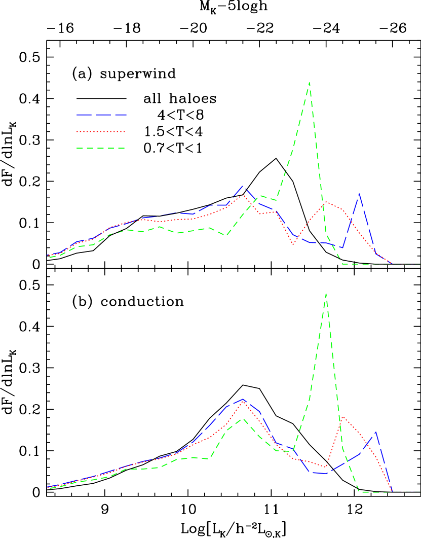
Figure 21: The fractional contribution of galaxies to iron enrichment as a function of $K$-band luminosity, $L_{K}$. Iron in all baryonic components (stars, cold gas, hot gas or ejected gas) is included, and the distributions are normalized to unit area. Panel (a) shows results for the superwind model and (b) for the conduction model. The long-dashed, dotted, and short-dashed lines indicate high, intermediate, and low temperature clusters, respectively. The solid lines show the distributions averaged over halos of all masses.

Finally, we examine which galaxies contribute the most to cluster metal enrichment. Fig. 21 shows the total amount of iron which galaxies have produced (either retained within the galaxy, injected into the ICM, or ejected from the cluster) as a function of their $K$-band luminosities at $z=0$. The contribution of each galaxy is calculated by summing the iron production over its formation history. The distributions over luminosity ${\rm d}F(\leq L_{K})/{\rm d}\ln L_{K}$ are then normalized to unit area. Results are shown for both the superwind and conduction models, and also split according to present-day cluster temperature. The solid line in each panel shows the iron production averaged over halos of all masses (including halos much smaller than clusters). These distributions are quite similar to the distributions of total stellar mass, which is expected since the mass of iron produced is closely related to the mass of stars formed. We also find that the normalized distributions for the mass of iron injected into the ICM are very similar to the distributions in Fig. 21 for the total mass of iron produced.

The distributions of iron production in Fig. 21 for the clusters show pronounced peaks at the high luminosity end. As the cluster mass or temperature increases, the position of the peak moves up in luminosity, but its amplitude decreases. This peak is produced by the central galaxies in the cluster halos, and reflects the distribution of total stellar mass (Benson et al., 2003b). The peak is most prominent for the lowest temperature clusters, because mergers are most effective at concentrating the stellar mass into a single central galaxy in such systems. Since the position of the peak due to central galaxies depends on halo mass, it is smeared out when we average over all halos, producing a smoother distribution (see the solid lines in Fig. 21).

We find that in the superwind model, half of the iron is produced by galaxies with luminosities $L_{K}$ brighter than $1.1\times 10^{11}$, $4.2\times 10^{10}$ and $3.6\times 10^{10}h^{-2}L_{\odot}$ for low, medium and high temperature clusters respectively, corresponding to galaxy stellar masses $5.4\times 10^{10}$, $2.2\times 10^{10}$ and $1.9\times 10^{10}h^{-1}M_{\odot}$ respectively. The median galaxy masses and luminosities for oxygen production are almost identical to those for iron. In the conduction model, the median galaxy masses and luminosities for metal production are somewhat higher: for iron production, the median K-band luminosities are $1.2\times 10^{11}$, $6.2\times 10^{10}$ and $5.4\times 10^{10}h^{-2}L_{\odot}$, and the median stellar masses are $7.3\times 10^{10}$, $3.5\times 10^{10}$ and $3.1\times 10^{10}h^{-1}M_{\odot}$ respectively, with very similar values for oxygen production. When we look at metal production averaged over halos of all masses, we find median luminosities $L_{K}$ for producing Fe or O of $4.2\times 10^{10}$ and $5.5\times 10^{10}h^{-2}L_{\odot}$ respectively for the superwind and conduction models, and median stellar masses of $1.8\times 10^{10}$ and $2.5\times 10^{10}h^{-1}M_{\odot}$ respectively. We thus see that the median K-band luminosity (or stellar mass) for metal production is similar (within a given model) for high mass clusters and field galaxies, but significantly larger in low mass clusters. For comparison, the characteristic luminosity of field galaxies in the K-band is $L_{K*}=6\times 10^{10}h^{-2}L_{\odot}$ (Cole et al., 2001). The metal production in clusters and in the field is thus predicted to be dominated by galaxies with $L_{K}\gtrsim L_{K*}$.

In our models, the median galaxy luminosities and masses for metal injection into the ICM are almost identical to those for metal production. Our median stellar masses for metal production are 2–3 times larger in the case of the most massive clusters than the median galaxy mass of $1\times 10^{10}h^{-1}M_{\odot}$ for metal (effectively oxygen) injection into the ICM calculated by De Lucia, Kauffmann & White (2004) for a $10^{15}h^{-1}M_{\odot}$ cluster. However, we are in agreement De Lucia et al. on the general conclusion that the ICM metal enrichment is dominated by fairly massive galaxies, in contrast to suggestions (e.g. Garnett, 2002) that metal ejection by dwarf galaxies has dominated the chemical enrichment of the ICM.

8 SUMMARY

We have investigated the metal enrichment of the ICM for clusters of different masses using a semi-analytical model of galaxy formation and evolution, galform (Cole et al. 2000). We have implemented in this model a detailed treatment of metal production by both SNe Ia and SNe II, based on the predictions of stellar evolution models for both stellar lifetimes and yields of different heavy elements. This enables us to follow the evolution of different elements (O, Mg, Si and Fe), including the long time delays for SNe Ia. Our model consistently calculates the cycling of gas and metals between stars, cold gas and hot gas. In order to reproduce the observed present-day galaxy luminosity function using a realistic baryon fraction in the models, we have considered two alternative mechanisms to prevent the overproduction of bright galaxies: (a) galactic superwinds which expel gas and metals from dark halos, with subsequent recapture in very massive halos, and (b) thermal conduction which transfers heat from the outer to the central regions of hot gas halos, thereby supressing gas cooling. We considered two different IMFs for bursts of star formation: the Kennicutt IMF that we also adopt for quiescent disk star formation, and a top-heavy, flat IMF with $x=0$. We have found that the form of the IMF is strongly constrained by the metal abundances of O, Mg, Si and Fe in the ICM. Our main conclusions can be summarized as follows:

1. A top-heavy IMF in starbursts is required in order to obtain ICM metal abundances as high as those observed, when the IMF for quiescent star formation in disks is fixed to be a standard, bottom-heavy IMF, such as the Kennicutt IMF. A burst IMF with $x=0$ reproduces the observed metal abundances in the ICM. We have also tried the Arimoto-Yoshii IMF with $x=1$ in bursts, and confirmed that it fails to produce sufficient metals. Considering that the IMF for quiescent star formation has been well constrained by many studies, including a semi-analytical model (Nagashima & Okamoto, 2004), this is strong evidence in support of a top-heavy IMF with $x\simeq 0$ in starbursts.

2. Both the superwind and conduction models reproduce the observed ICM metal abundances and abundance ratios. The superwind model predicts lower metal abundances in low temperature ($T\la 1$ keV) clusters. Therefore if the drop in [Fe/H] for clusters with $T\la 1$ keV found using ASCA is real, this could be evidence for the action of superwinds. The current data are still limited, however, so future observations, particularly of low temperature clusters, would strongly constrain the superwind model.

3. Our model is in broad agreement with the observed ratio of ICM gas mass to the total $b_{\rm J}$-band stellar luminosity in clusters, $M_{\rm hot}/L_{b_{\rm J}}$. In particular, the superwind model predicts a decrease of $M_{\rm hot}/L_{b_{\rm J}}$ in low temperature clusters, as is observed, because the superwind expels gas from these clusters.

4. The iron metallicity, [Fe/H], is predicted to decrease only slowly with increasing redshift. The difference in [Fe/H] between $z=0$ and 1 is at most 0.2 dex. This mild evolution is broadly consistent with the recent observations by Tozzi et al. (2003). In contrast with [Fe/H], [O/H] is almost independent of redshift over this range, so [O/Fe] increases with redshift.

5. The metal production histories of clusters having the same present-day mass are very similar. In contrast, the cluster mass assembly histories show a wide variety. This suggests that the variety of metallicity gradients observed in clusters may be caused not only by observational errors but also by the variety of assembly histories. Presumably this is the origin of the diversity in the observed metallicities of present-day clusters, because most observations measure metallicities only at cluster centres.

6. In clusters and in the field, metal production is dominated by galaxies with K-band luminosities similar to or brighter than $L_{*}$. In low-mass clusters, the contribution of the central galaxy to metal production is very important, but this effect is weaker in high-mass clusters.

Throughout this paper, we have neglected any contribution of intracluster stars to the metal enrichment of the ICM, since in our model all stars are in galaxies. Based on recent measurements of the intracluster light, it has been suggested that intracluster stars might have produced a large fraction of the iron observed in the ICM (Zaritsky, Gonzalez & Zabludoff, 2004). The intracluster stars would presumably originate from material tidally stripped from galaxies or ejected during violent mergers, so the luminosity function of galaxies in clusters would also be affected. In our model, tidal stripping of stars from galaxies would not affect the total mass of iron produced (if all other parameters remain the same), but it might affect the fraction of the iron which is ejected into the ICM. This possibility clearly deserves further observational and theoretical study.

It is also evident that, in order to better constrain our model, we need more accurate ICM metallicity measurements for larger samples of clusters. These measurements need to cover the outer parts of clusters as well as the central regions, in order derive accurate global metallicities. The observational situation will be substantially improved by the Astro-E2 satellite scheduled for launch in 2005, as well as by further data from XMM-Newton and Chandra. Further constraints on the model can be obtained by examining the abundances of different heavy elements in galaxies, and we will investigate this latter topic in future papers.

Appendix A Correction of the observational data for metallicity gradients

Some clusters are known to have substantial metallicity gradients. The so-called ‘cooling flow’ clusters show enhancements in the metallicities of some elements toward the cluster centre (e.g., Tamura et al., 2001; Matsushita, Finoguenov & Böhringer, 2003; De Grandi et al., 2004). Tamura et al. (2001, 2004) have reported that in cooling flow clusters O and Mg among the $\alpha$ elements do not show the metallicity gradients, whereas Fe and Si tend to show gradients, at least from the cluster centre to around half of the virial radius, despite the fact that Si is an $\alpha$ element. Non-cooling flow clusters generally do not show metallicity gradients for any elements. Our model predicts the global metallicity of the ICM, averaged over the whole cluster. Therefore we need to correct the observed metallicities to obtain values averaged over the whole cluster, because most observations give only central values.

De Grandi et al. (2004) compiled Fe metallicity gradients in 12 cooling flow clusters. Based on their results, we assume that all cooling flow clusters have the same shape of metallicity gradients in both Fe and Si,

$$Z(r)=Z_{0}\left[1+\left(\frac{x}{x_{c}}\right)^{2}\right]^{-\alpha},$$ (23)

where $x=r/r_{200}$, $r_{200}$ is the radius within which the mean overdensity is 200 times the critical density, $x_{c}=0.04$ and $\alpha=-0.18$. We define the average metallicity within radius $r$ as,

$$\bar{Z}(\leq r)=\frac{\int_{0}^{r}Z(r)\rho_{g}(r)r^{2}dr}{\int_{0}^{r}\rho_{g}(r)r^{2}dr},$$ (24)

where $\rho_{g}(r)$ is the gas density. We assume that the observed metallicities correspond to average values within some radius $r$, $\bar{Z}(\leq r)$, and then use the assumed form of the metallicity profile (equation (eqn:metalgrad))to correct these to mean values $\bar{Z}(\leq r_{\rm vir})$ within the virial radius $r_{\rm vir}$. The central metallicity $Z_{0}$ is thus treated as a parameter chosen so as to match an observed metallicity $\bar{Z}(\leq r)$.

A.1 De Grandi et al.’s sample

De Grandi et al. (2004) give the iron masses of individual clusters as a function of $\Delta$, which is a spherical overdensity,

$$\Delta=\frac{3M_{\rm tot}(<r_{\Delta})}{4\pi\rho_{c,z}r_{\Delta}^{3}},$$ (25)

where $M_{\rm tot}(<r)$ is the total mass within a radius $r$ and $\rho_{c,z}$ is the critical density of the universe at redshift $z$. Using the data on the distributions of total and gas mass given by Ettori, De Grandi & Molendi (2002), we obtain an averaged metallicity for each cluster within $r_{\Delta}$, $\bar{Z}(\leq r_{\Delta})$. The gas density distribution, $\rho_{g}(r)$ is assumed to follow an isothermal profile with a core,

$$\rho_{g}(r)\propto\left[1+\left(\frac{r}{r_{s}}\right)^{2}\right]^{-1}.$$ (26)

To obtain $r_{\Delta}$, we use the structural parameters given by Ettori, De Grandi & Molendi (2002) assuming an NFW profile (Navarro, Frenk & White, 1997) for the total density distribution. We have found that the use of structural parameters assuming a King profile hardly affects averaged metallicities. $r_{s}$ is assumed to be the same as the scale radius of the NFW profile, but the results are not sensitive to the exact value chosen.

The metallicity at the cluster centre, $Z_{0}$ in eq.(23), depends on the individual cluster. Using the above equations and the values at $r_{2500}$, at which the observed data are given in the above papers, we obtain the average metallicity $\bar{Z}$ within the virial radius ($r\leq r_{\rm vir}$, corresponding to $\Delta\simeq 100$ in a $\Lambda$CDM universe),

$$\bar{Z}=\frac{M_{{\rm Fe},2500}}{M_{{\rm gas},2500}}\frac{\bar{Z}(\leq r_{\rm vir})}{\bar{Z}(\leq r_{2500})}.$$ (27)

The average [Fe/H] is easily estimated from $\bar{Z}$.

A.2 Peterson et al.’s sample

Peterson et al. (2003) observed only the central parts of clusters within a $1^{\prime}$ angular radius. Their observed metallicities of Fe and Si are assumed to correspond to $\bar{Z}(\leq r_{1^{\prime}})$, where $r_{1^{\prime}}$ is the radius at which the angular size is equal to 1 arcmin. The average metallicity within the virial radius is then obtained from

$$\bar{Z}=Z_{\rm obs}\frac{\bar{Z}(\leq r_{\rm vir})}{\bar{Z}(\leq r_{1^{\prime}})}.$$ (28)

The parameters regarding redshift and structure required to obtain averaged metallicities are tabulated in their paper.

Recent observations suggest that the metallicity gradients of Si are very similar to those of Fe (Tamura et al., 2001, 2004; Matsushita, Finoguenov & Böhringer, 2003). Therefore we assume that Si has the same shape of metallicity profile as Fe. As already mentioned, because O and Mg seem not to have any metallicity gradients, we regard the observed values of central metallicities as equivalent to the metallicities averaged over the whole cluster.

A.3 Fukazawa et al.’s sample

The measurements of Fe and Si abundances by Fukazawa et al. (1998) include data from the outer parts of the clusters. We therefore assume that their abundance measurements are close to global averages, and do not apply any corrections.

A.4 Baumgartner et al.’s sample

Baumgartner et al. (2003) obtained average abundances of several elements, including Fe and Si, in bins of cluster temperature by performing a stacking analysis of observations of 273 clusters from the ASCA archives. Although their cluster sample is large, metallicity gradients combined with the large point spread function for ASCA cause problems for interpreting their results, especially for Fe. The iron abundance is usually estimated from the Fe-K or Fe-L lines. For high-temperature clusters, the photon flux in the Fe-K line is larger than that in the Fe-L line, and the Fe-K line yields accurate measurements of the iron abundance. On the other hand, for low and intermediate temperature clusters, the Fe-K line becomes very weak, and the photon flux is larger in the Fe-L line, so the Fe-L line dominates in abundance estimates. Lower temperature gas emits more photons in the Fe-L line than in the Fe-K line. This has the consequence that for clusters with cooling cores, the observationally-estimated iron abundance is weighted towards the value in the low temperature component, that is, the central region, where the iron abundance is typically higher than the average over the whole cluster. Thus, as Fukazawa et al. (1998) have done, the data for the central region should be removed to get a fairer estimate of the metallicity averaged over the whole cluster. Baumgartner et al. (2003) have not done this, and this may be the reason why their data show an enhancement of the iron metallicity at intermediate cluster temperatures. For this reason, we do not include their data on Fe abundances in our comparison with the models. Their data on Si abundances seem to be less affected by this problem, so we do include those data in our comparison.

References

- Anders & Grevesse (1989) Anders E., Grevesse N., 1989, Geochim. Cosmochim. Acta, 53, 197
- Arimoto & Yoshii (1987) Arimoto N., Yoshii Y., 1987, A&A, 173, 23
- Baugh et al. (2004a) Baugh C.M., et al. (the 2dFGRS team), 2004a, MNRAS, 351, L44
- Baugh et al. (2004b) Baugh C.M., Lacey C.G., Frenk C.S. Granato G.L. Silva L., Bressan A., Benson A.J., Cole S., 2004b, MNRAS, in press (astro-ph/0406069) (B04)
- Baumgartner et al. (2003) Baumgartner W.H., Loewenstein M., Horner D.J., Mushotzky R.F., 2003, ApJ, submitted (astro-ph/0309166)
- Bell et al. (2003) Bell E.F., McIntosh D.H., Katz N., Weinberg M.D., 2003, ApJ, 149, 289
- Benson et al. (2003a) Benson A. J., Bower R.G., Frenk C. S., Lacey C. G., Baugh C. M., Cole S., 2003a, ApJ, 599, 38
- Benson et al. (2003b) Benson A.J., Frenk C.S., Baugh C.M., Cole S., Lacey C.G., 2003b, MNRAS 343, 679
- Cole (1991) Cole S., 1991, ApJ, 367, 45
- Cole et al. (1994) Cole S., Aragon-Salamanca A., Frenk C. S., Navarro J. F., Zepf S. E., 1994, MNRAS, 271, 781
- Cole et al. (2000) Cole S., Lacey C. G., Baugh C. M., Frenk C. S., 2000, MNRAS, 319, 168 (CLBF)
- Cole et al. (2001) Cole S. et al. 2001, MNRAS, 2001, 326, 225
- David, Forman & Jones (1991) David L.P., Forman W., Jones C., 1991, ApJ, 380, 39
- De Grandi & Molendi (2002) De Grandi S., Molendi S., 2002, ApJ, 567, 163
- De Grandi et al. (2004) De Grandi S., Ettori S., Longhetti M., Molendi S., 2004, A&A, 419, 7
- De Lucia, Kauffmann & White (2004) De Lucia, G., Kauffmann, G. & White, S.D.M., 2004, MNRAS, 349, 1101
- Eke et al. (1996) Eke V.R., Cole S., Frenk C.S., 1996, MNRAS, 282, 263
- Enoki, Nagashima & Gouda (2003) Enoki M., Nagashima M., Gouda N., 2003, PASJ, 55, 133
- Ettori, De Grandi & Molendi (2002) Ettori S., De Grandi S., Molendi S., 2002, A&A, 391, 841
- Fukazawa et al. (1998) Fukazawa Y., Makishima K., Tamura T., Ezawa H., Xu H., Ikebe Y., Kikuchi K., Ohashi T., 1998, PASJ, 50, 187
- Garnett (2002) Garnett, D.R., 2002, ApJ, 581, 1019
- Gibson & Matteucci (1997a) Gibson B.K., Matteucci F., 1997a, MNRAS, 291, L8
- Gibson & Matteucci (1997b) Gibson B.K., Matteucci F., 1997b, ApJ, 475, 47
- Granato et al. (2004) Granato G.L., De Zotti G., Silva L., Bressan A., Danese L., 2004, ApJ, 600, 580.
- Greggio & Renzini (1983) Greggio L., Renzini A., 1983, A&A, 118, 217
- Grevesse & Sauval (1998) Grevesse N., Sauval A.J., 1998, Space Sci. Rev., 85, 161
- Hatton et al. (2003) Hatton, S., Devriendt, J.E.G., Ninin, S., Bouchet, F.R., Guiderdoni, B., Vibert, D., 2003, MNRAS, 343, 75
- Helly et al. (2003) Helly J.C., Cole S., Frenk C.S., Baugh C.M., Benson A.J., Lacey C.G., 2003, MNRAS, 338, 903
- Huang et al. (2003) Huang J.-S., Glazebrook K., Cowie L.L., Tinney C., 2003, ApJ, 584, 203
- Irwin & Bregman (2001) Irwin J.A., Bregman J.N., 2001, ApJ, 546, 150
- Jenkins et al. (2001) Jenkins A., Frenk C. S., White S. D. M., Colberg J. M., Cole S., Evrard A. E., Couchman H. M. P., Yoshida N. 2001, MNRAS, 321, 372
- Kauffmann (1996) Kauffmann G., 1996, MNRAS, 281, 475
- Kauffmann & Charlot (1998) Kauffmann G., Charlot S., 1998, MNRAS, 294, 705
- Kauffmann & Haehnelt (2000) Kauffmann G., Haehnelt M., 2000, MNRAS, 311, 576
- Kauffmann, White & Guiderdoni (1993) Kauffmann G., White S. D. M., Guiderdoni B., 1993, MNRAS, 264, 201
- Kennicutt (1983) Kennicutt R.C., 1983, ApJ, 272, 54
- Kroupa (2002) Kroupa P., 2002, Sci., 295, 82
- Lacey & Cole (1993) Lacey C.G., Cole S., 1993, MNRAS 262, 627
- Lacey et al. (2005) Lacey C.G., et al. 2005, in preparation
- Larson (1969) Larson R.B., 1969, MNRAS, 145, 297
- Lia, Portinari & Carraro (2002) Lia C., Portinari L., Carraro G., 2002, MNRAS, 330, 821
- Loewenstein & Mushotzky (1996) Loewenstein M., Mushotzky R.F., 1996, ApJ, 466, 695
- Maoz & Gal-Yam (2004) Maoz D., Gal-Yam A., 2004, MNRAS, 347, 951
- Marigo (2001) Marigo P., 2001, A&A, 370, 194
- Matsushita, Ohashi & Makishima (2000) Matsushita K., Ohashi T., Makishima K., 2000, PASJ, 52, 685
- Matsushita, Finoguenov & Böhringer (2003) Matsushita K., Finoguenov A., Böhringer H., 2003, A&A, 401, 443
- Matteucci & Gibson (1995) Matteucci F., Gibson B.K., 1995, A&A, 304, 11
- Matteucci & Greggio (1986) Matteucci F., Greggio L., 1986, MNRAS, 154, 279
- Matteucci & François (1989) Matteucci F., François P., 1989, MNRAS, 239, 885
- Menci et al. (2002) Menci N., Cavaliere A., Fontana A., Giallongo E., Poli F., 2002, ApJ, 575, 18
- Moretti, Portinari & Chiosi (2003) Moretti A., Portinari L., Chiosi C., 2003, A&A, 408, 431
- Mushotzky et al. (1996) Mushotzky R., Loewenstein M., Arnaud K.A., Tamura T., Fukazawa Y., Matsushita K., Kikuchi K., Hatsukade I., 1996, ApJ, 466, 686
- Nagashima & Gouda (2001) Nagashima M., Gouda N., 2001, MNRAS, 325, L13
- Nagashima & Okamoto (2004) Nagashima M., Okamoto T., 2004, submitted (astro-ph/0404486)
- Nagashima et al. (2001) Nagashima M., Totani T., Gouda N., Yoshii Y., 2001, ApJ, 557, 505
- Nagashima et al. (2002) Nagashima M., Yoshii Y., Totani T., Gouda N., 2002, ApJ, 578, 675
- Nagashima & Yoshii (2004) Nagashima M., Yoshii Y., 2004, ApJ, 610, 23
- Nagashima et al. (2005) Nagashima M., et al. 2005, in preparation
- Navarro, Frenk & White (1997) Navarro J.F., Frenk C.S., White S.D.M., 1997, ApJ, 490, 493
- Nomoto et al. (1997) Nomoto K., Iwamoto K., Nakasato N., Thielemann F.-K., Brachwitz F., Tsujimoto T., Kubo Y., Kishimoto N., 1997, Nuclear Physics, A621, 467c
- Norberg et al. (2002) Norberg P., et al. (the 2dFGRS team), 2002, MNRAS, 336, 907
- Okoshi et al. (2004) Okoshi K., Nagashima M., Gouda N., Yoshioka S., 2004, ApJ, 603, 12
- Pagel & Tautvaišienė (1995) Pagel B.E.J., Tautvaišienė G., 1995, MNRAS, 276, 505
- Peacock et al. (2001) Peacock J.A., et al. (the 2dFGRS team), 2001, Nature, 410, 169.
- Percival et al. (2002) Percival W.J., et al. (the 2dFGRS team), 2002, MNRAS, 337, 1068
- Peterson et al. (2001) Peterson J.R., et al., 2001, A&A, 365, L104
- Peterson et al. (2003) Peterson J.R., Kahn S.M., Paerels F.B.S., Kaastra J.S., Tamura T., Bleeker J.A.M., Ferrigno C., Jernigan J.G., 2003, ApJ, 590, 207
- Portinari, Chiosi & Bressan (1998) Portinari L., Chiosi C., Bressan A., 1998, A&A, 334, 505
- Press & Schechter (1974) Press W., Schechter P., 1974, ApJ, 187, 425
- Renzini et al. (1993) Renzini A., Ciotti L., D’Ercole A., Pellegrini S., 1993, ApJ, 419, 52.
- Salpeter (1955) Salpeter E.E., 1955, ApJ, 121, 161
- Sanderson et al. (2003) Sanderson A.J.R., Ponman T.J., Finoguenov A., Lloyd-Davies E.J., Markevitch M., 2003, MNRAS, 340, 989
- Sanderson & Ponman (2003) Sanderson A.J.R., Ponman T.J., 2003, MNRAS, 345, 1241
- Smith & Gallagher (2001) Smith L.J., Gallagher III J.S., 2001, MNRAS, 326, 1027
- Somerville & Primack (1999) Somerville R.S., Primack J. R., 1999, MNRAS, 310, 1087
- Somerville, Primack & Faber (2001) Somerville R.S., Primack J. R., Faber S.M., 2001, MNRAS, 320, 504
- Spergel et al. (2003) Spergel D.N., et al. (the WMAP Team), 2003, ApJS, 148, 175
- Takahara & Takahara (1981) Takahara M., Takahara F., 1981, PTP, 65, 369
- Tamura et al. (2001) Tamura T., Bleeker J.A.M., Kaastra J.S., Ferrigno C., Molendi S., 2001, A&A, 379, 107
- Tamura et al. (2004) Tamura T., Kaastra J.S., den Herder J.W.A., Bleeker J.A.M., Peterson J.R., 2004, A&A, 420, 135
- Thomas (1999) Thomas D., 1999, MNRAS, 306, 655
- Thomas, Greggio & Bender (1998) Thomas D., Greggio L., Bender R., 1998, MNRAS, 296, 119
- Thomas & Kauffmann (1999) Thomas D., Kauffmann G., 1999, in Spectrophotometric dating of stars and galaxies, ed. I. Hubeny, S. Heap & R. Cornett, Vol. 192 (ASP Conf. Ser.), 261
- Timmes, Woosley & Weaver (1995) Timmes F.X., Woosley S.E., Weaver T.A., 1995, ApJS, 98, 617
- Tornatore et al. (2004) Tornatore L., Borgani S., Matteucci F., Recchi S., Tozzi P., 2004, MNRAS, 349, 19
- Tozzi et al. (2003) Tozzi P., Rosati P., Ettori S., Borgani S., Mainieri V., Norman C., 2003, ApJ, 593, 705
- Tsujimoto et al. (1995) Tsujimoto T., Nomoto K., Yoshii Y., Hashimoto M., Yanagida Y., Thielemann F.-K., 1995, MNRAS, 277, 945
- Tsuru et al. (1997) Tsuru T.G., Awaki H., Koyama K., Ptak A., 1997, PASJ, 49, 619
- Valdarnini (2003) Valvarnini R., 2003, MNRAS, 339, 1117
- Whelan & Iben (1973) Whelan, J., Iben, I., 1973, ApJ, 186, 1007
- White & Frenk (1991) White, S.D.M. & Frenk, C.S., 1991, ApJ, 379, 52
- Yoshida et al. (2002) Yoshida N., Stoehr F., Springel V., White S.D.M., 2002, MNRAS, 335, 762
- Yoshii, Tsujimoto & Nomoto (1996) Yoshii Y., Tsujimoto T., Nomoto K., 1996, MNRAS, 462, 266
- Zaritsky, Gonzalez & Zabludoff (2004) Zaritsky D., Gonzalez A.H., Zabludoff A.I., 2004, ApJ, in press (astro-ph/0406291)
- Zepf & Silk (1996) Zepf S.E., Silk J., 1996, ApJ, 466, 114