Diffusive Shock Acceleration in Unmodified Relativistic, Oblique Shocks

Abstract

We present results from a fully relativistic Monte Carlo simulation of diffusive shock acceleration (DSA) in unmodified shocks. The computer code uses a single algorithmic sequence to smoothly span the range from nonrelativistic speeds to fully relativistic shocks of arbitrary obliquity, providing a powerful consistency check. While known results are obtained for nonrelativistic and ultra-relativistic parallel shocks, new results are presented for the less explored trans-relativistic regime and for oblique, fully relativistic shocks. We find, for a wide trans-relativistic range extending to shock Lorentz factors $>30$, that the particle spectrum produced by DSA varies strongly from the canonical $f(p)\propto p^{-4.23}$ spectrum known to result in ultra-relativistic shocks. Trans-relativistic shocks may play an important role in $\gamma$-ray bursts and other sources and most relativistic shocks will be highly oblique.

1 Introduction

Relativistic shocks, and their associated energetic particles resulting from diffusive particle acceleration, have received considerable attention in recent years (e.g., Ostrowski, 1993; Achterberg et al., 2001; Ellison & Double, 2002; Meli & Quenby, 2003a; Niemiec & Ostrowski, 2004). This is due primarily to their likely presence in extreme space phenomena, in particular $\gamma$-ray bursts (GRBs) (e.g., Piran, 1999; Rees, 2000), and their possible role in producing ultra-high-energy cosmic rays (UHECRs) (e.g., Waxman, 2000). While most work on diffusive shock acceleration (DSA) in relativistic shocks has been restricted to the ultra-relativistic regime with magnetic fields assumed parallel to the shock normal, trans-relativistic shocks are certain to be important in some sources and, in general, relativistic shocks will have highly oblique magnetic fields. Here we consider test-particle diffusive shock acceleration in shocks of arbitrary obliquity and with arbitrary Lorentz factors, $\gamma_{0}$, ranging from nonrelativistic shocks to fully relativistic ones.

Diffusive shock acceleration in relativistic, oblique shocks was initially addressed by Kirk & Heavens (1989) and Ballard & Heavens (1991) both analytically and numerically, and by Ostrowski (1991), using numerical techniques. Ostrowski (1993) further investigated oblique, relativistic shocks using small perturbations superimposed on a uniform magnetic field, and Bednarz & Ostrowski (1996) investigated the corresponding time-scale for test-particle acceleration. Bednarz & Ostrowski (1998) determined the energy spectra of accelerated test particles in oblique, ultra-relativistic shocks with results leading to a limiting energy spectral index of $\sigma_{E}=2.3\pm 0.1$, independent of shock obliquity. This result had been anticipated by Heavens & Drury (1988) for test-particle acceleration in ultra-relativistic, parallel shocks. More recent work on oblique, relativistic shock acceleration has been presented by Meli (2002), Meli & Quenby (2003b) and Niemiec & Ostrowski (2004).

Despite the emphasis on ultra-relativistic shocks in theoretical work, trans-relativistic shocks may play an important role in GRBs, both for internal shocks and for the expanding fireball shock presumably responsible for the afterglow. Even though GRB fireballs may initially have Lorentz factors $\gamma_{0}>100$, the internal shocks, credited by many as responsible for converting the bulk kinetic energy of expansion into particle internal energy and hence to radiation, may be much slower with $\gamma_{0}$’s of a few. As the fireball expands into the ambient interstellar medium, regardless of its initial $\gamma_{0}$, it will slow and pass through a trans-relativistic phase before becoming nonrelativistic. Existing afterglow observations span this phase and understanding Fermi acceleration in trans-relativistic shocks is important for interpreting the observed emission.

Considering the importance of oblique, trans-relativistic shocks, we have extended our well-tested Monte Carlo model of DSA (e.g., Ellison, Jones, & Reynolds, 1990; Jones & Ellison, 1991; Ellison & Double, 2002) to include shocks of arbitrary obliquity and speed. We describe the details of the model and present results for shocks with parameters not previously addressed in published work. In the two extreme cases where direct comparisons can be made – nonrelativistic and ultra-relativistic shocks – our results are consistent with previous work. In future studies we will investigate nonlinear effects in oblique relativistic shocks where accelerated particles modify the shock structure (e.g., Ellison & Double, 2002). Here we consider only particle acceleration in plane, unmodified shocks where effects on the shock structure from superthermal particles are ignored.

In contrast to nonrelativistic shocks, the details of particle scattering strongly influence the superthermal particle populations produced in trans-relativistic and ultra-relativistic shocks (e.g., Bednarz & Ostrowski, 1996, 1998). Unfortunately, these details are not known with any reliability so the results of all current models of DSA depend on the particular scattering assumptions made. We use a simple, parameterized model of particle diffusion and attempt to describe our procedures in sufficient detail so readers can clearly see how the assumptions influence the particle distribution functions. While we make no claim that our scattering scheme is more realistic than other models, some of which are far more complex (e.g., Niemiec & Ostrowski, 2004), we do believe it adequately parameterizes the particle transport. Until a self-consistent theory of wave-particle interactions in relativistic shocks is produced, parameterization will be necessary.

Unlike most other models of DSA, we follow particles from thermal energies through the injection process to superthermal energies. While not necessary in test-particle calculations, some description of the injection process from thermal energies must be used in self-consistent, nonlinear calculations. The procedures we use to model injection in relativistic shocks are identical to those we have used with some success in nonrelativistic shocks (e.g., Ellison, Möbius, & Paschmann, 1990; Jones & Ellison, 1991; Baring et al., 1997).

Finally, while our results are applicable to ion acceleration in GRBs and the possible production of UHECRs, they are not directly applicable to the photon emission for two basic reasons. The first is that energy budget requirements of GRB models generally require extremely efficient conversion of the bulk kinetic energy of the fireball into radiation. This means that the particle acceleration process must be efficient and, therefore, self-consistent, nonlinear models must be used instead of the test-particle ones we present here.

Second, the radiation seen from GRBs is produced by electrons not protons. Normal non-relativistic DSA in a proton-electron plasma will always put more energy into protons than electrons. In relativistic shocks, the fraction of energy going into electrons is reduced dramatically. In order to determine the distribution of energy between protons and electrons for GRBs, a two-component acceleration model must be done in the nonlinear regime. This requires additional assumptions for the electron injection and, to obtain results even remotely consistent with GRB properties, requires the modeling of lepton dominated plasmas. Preliminary work for lepton dominated parallel shocks is given in Double (2003).

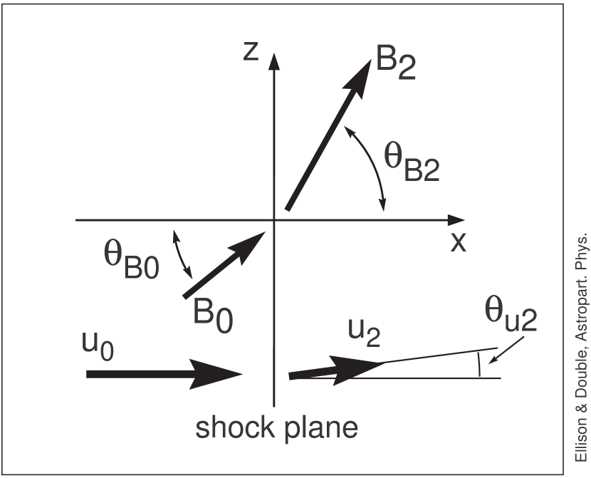
Figure 1: Plane shock geometry where the shock lies in the $y$-$z$ plane.

2 Monte Carlo Simulation of DSA

Many of the details of the model we use here have been described previously in the context of nonrelativistic, oblique shocks (e.g., Ellison, Baring, & Jones, 1996; Ellison, Jones, & Baring, 1999), or relativistic, parallel shocks (Ellison & Double, 2002). We refer to this previous work and describe in greater detail those aspects that are being presented for the first time.

2.1 Jump conditions

We let $u_{0}$ be the flow speed of the unshocked (i.e., upstream) plasma as measured in a frame at rest with the shock. For convenience, we assume the unshocked flow is normal to the shock along the $x$-direction so that $u_{0}=u_{x0}$. The shock Lorentz factor is then $\gamma_{0}=[1-(u_{0}/c)^{2}]^{-1/2}$, where $c$ is the speed of light. Downstream, the flow will, in general, have a $z$-component as well, i.e., $u_{2}=\sqrt{u_{x2}^{2}+u_{z2}^{2}}$ (see Fig. 1). For nonrelativistic shocks, the jump conditions, i.e., the downstream density $\rho_{2}$, flow speed $u_{2}$, pressure $P_{2}$, and magnetic field $B_{2}$, in terms of given upstream values, are well-known. For trans-relativistic shocks, however, the jump conditions are not straightforward and can only be determined numerically. In all of the examples given here, except where specifically noted, we assume high sonic and Alfvén Mach numbers and use the results of Double et al. (2004) to calculate the jump conditions.

The primary jump conditions come from the equation of continuity which gives the compression ratio $r=u_{x0}/u_{x2}=\gamma_{2}\rho_{2}/(\gamma_{0}\rho_{0})$, and the electromagnetic boundary condition which determines the angle the downstream magnetic field makes with the shock normal, $\theta_{\mathrm{B2}}$. Here, $\gamma_{2}=[1-(u_{2}/c)^{2}]^{-1/2}$ and note that only the components of flow speed along the shock normal are used in the definition of r.

2.2 Test-particle power law

For nonrelativistic shock speeds, the test-particle power law from DSA is well-known and is given by:

$$f(p)\,d^{3}p\propto p^{-\sigma_{\mathrm{TP}}}\,d^{3}p\ ;\quad\sigma_{\mathrm{TP}}=3r/(r-1)\ ,$$ (1)

where $p$ is momentum and $f(p)\,d^{3}p$ is the rotationally averaged, isotropic number density of particles in $d^{3}p$ (Krymsky, 1977; Axford, Leer, & Skadron, 1977; Blandford & Ostriker, 1978; Bell, 1978). For high sonic and Alfvén Mach number, nonrelativistic, unmodified shocks, the compression ratio $r\simeq 4$ and the test-particle power-law index $\sigma_{\mathrm{TP}}$, is also approximately 4. One of the remarkable aspects of test-particle DSA is that for $v_{p}\gg u_{0}$, where $v_{p}$ is the particle speed measured in the local plasma frame, $\sigma_{\mathrm{TP}}$ depends only on $r$ regardless of the diffusive properties of the plasma and eqn. (1) holds regardless of the shock obliquity (e.g., Blandford & Ostriker, 1978). In other words, provided that the particles are nearly isotropic simultaneously in the upstream, shock, and downstream reference frames, eqn. (1) holds.

For relativistic shocks, $u_{0}\sim c$ and particle distributions are not isotropic across reference frames. This does not change the physics of the shock acceleration mechanism – particles still gain energy by scattering back and forth across the shock – but it does make obtaining analytic descriptions of the acceleration process far more difficult because the diffusion approximation can no longer be made. There are two important consequences of this. First, Monte Carlo computer simulation techniques, which do not need to make any assumption concerning the isotropy of the particle distributions, become the method of choice for studying particle acceleration (e.g., Kirk & Schneider, 1987; Ellison, Jones, & Reynolds, 1990; Ostrowski, 1991; Achterberg et al., 2001; Ellison & Double, 2002; Meli & Quenby, 2003a), and second, due to the mathematical difficulties, there are no analytic solutions to compare computer simulation results to as there are with nonrelativistic shocks.

2.3 Details of the Monte Carlo method

Monte Carlo techniques, while straightforward in principle, are, in fact, difficult in practice with many subtle features which can produce errors if not implemented properly. To minimize the possibility of error, we employ a code which has a single algorithmic sequence regardless of $\gamma_{0}$, $\theta_{\mathrm{B0}}$, or scattering parameters. This allows us to smoothly span the parameter space from nonrelativistic flow speeds, where analytic solutions exist, through the trans-relativistic regime where analytic solutions do not exist, to ultra-relativistic shocks, where canonical results again exist for parallel shocks. While a smooth transition between known results is not a sufficient condition to guarantee accuracy, it is a necessary condition for correct results.

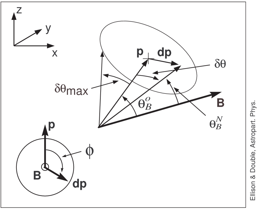
Figure 2: Schematic representation of pitch-angle diffusion.

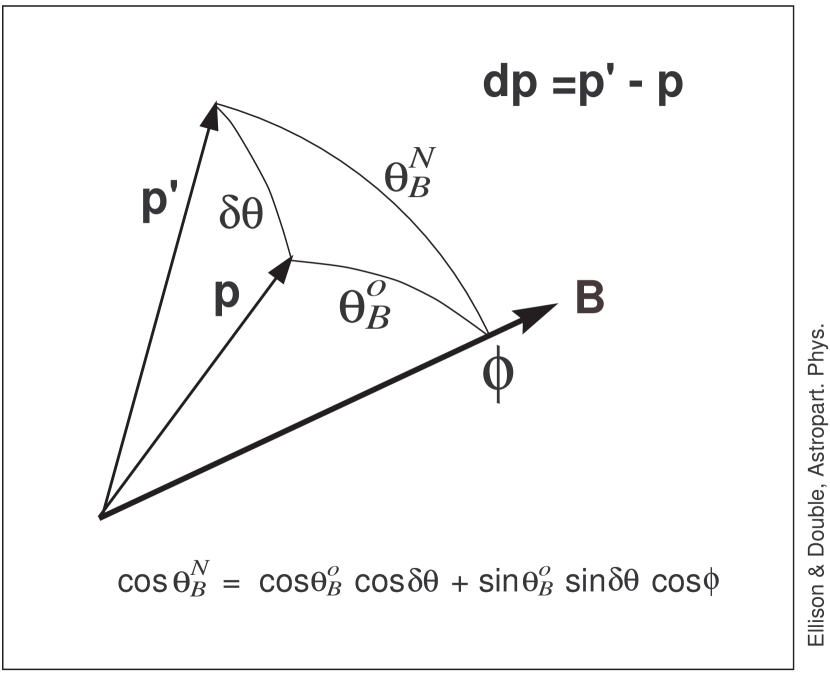
Figure 3: Spherical triangle representation of a scattering event where the momentum changes from p to $\mathbf{p^{\prime}}$ and a particle’s pitch angle changes from $\theta_{B}^{0}$ to $\theta_{B}^{N}$.

2.3.1 Particle diffusion and convection

Our implementation of pitch-angle diffusion is described in detail in Ellison, Jones, & Reynolds (1990) and Ellison, Baring, & Jones (1996). We assume that scattering is elastic and isotropic in the local plasma frame and that the scattering mean free path $\lambda$ in the local frame is proportional to the gyroradius $r_{g}$. We simulate small-angle scattering by allowing the tip of the particle’s fluid-frame momentum vector $\mathbf{p}$ to undergo a random walk on the surface of a sphere (see Fig. 2). If the particle originally had a pitch angle ${\theta_{B}^{0}=\arccos\{{\bf p}\cdot{\bf B}/|{\bf p}|\,|{\bf B}|\}}$, and after a time ${\delta t}$ undergoes a small change in direction of magnitude ${\delta\theta}$, its new pitch angle, ${\theta_{B}^{N}}$, is related to the old by

$$\cos\theta_{B}^{N}=\cos\theta_{B}^{0}\cos{\delta\theta}+\sin{\theta_{B}^{0}}\sin{\delta\theta}\cos{\phi}\ ,$$ (2)

where $\,\phi\,$ is the azimuthal angle of the momentum change $d\mathbf{p}$ measured relative to the plane defined by the original momentum $\,{\bf p}\,$ and $\,{\bf B}\,$ (see Fig. 3). After each scattering, a new phase angle around the magnetic field, $\,\phi_{B}^{N}\,$, is determined from the old phase angle, $\,\phi_{B}^{0}\,$, by

$$\phi_{B}^{N}=\phi_{B}^{0}+\arcsin\left[\hbox{${{\displaystyle\sin{\phi}\,\sin{\delta\theta}\vphantom{(}}\over{\displaystyle\sin{\theta_{B}^{N}}\vphantom{(}}}$}\right]\ ,$$ (3)

where $\cos{\delta\theta}$ is randomly chosen from a uniform distribution between 1 and $\cos{\delta\theta_{\rm max}}$, and $\,\phi\,$ is randomly chosen from a uniform distribution between $-\pi$ and $\pi$, so that the tip of the momentum vector walks randomly over the surface of a sphere of radius $\,p=|{\bf p}|\,$.

If the time in the local frame required to accumulate deflections of the order of $90^{\circ}$ is identified with the collision time $t_{c}=\lambda/v_{p}$, Ellison, Jones, & Reynolds (1990) showed that

$$\delta\theta_{\rm max}=\sqrt{6\delta t/t_{c}}\ ,$$ (4)

where $\delta t$ is the time between pitch-angle scatterings. We take $\lambda$ proportional to the gyroradius $r_{g}=pc/(eB)$ ($e$ is the electronic charge and $B$ is the local uniform magnetic field in Gaussian units), i.e., $\lambda=\eta_{\mathrm{mfp}}\,r_{g}$, where $\eta_{\mathrm{mfp}}$ is a measure of the “strength” of scattering. The strong scattering limit, $\eta_{\mathrm{mfp}}=1$, is called Bohm diffusion. Now, setting $\delta t=\tau_{g}/N_{g}$, where $N_{g}\gg 1$ is the number of gyro-time segments $\delta t$, dividing a gyro-period $\tau_{g}=2\pi r_{g}/v_{p}$, we have

$$\delta\theta_{\rm max}=\sqrt{12\pi/(\eta_{\mathrm{mfp}}N_{g})}\ ,$$ (5)

and the scattering properties of the medium are modeled with the two parameters $\eta_{\mathrm{mfp}}$ and $N_{g}$.

An important limitation of this scheme is the assumption of elastic scattering which implies that the scattering centers are frozen into the fluid. This eliminates both the possibility of second-order Fermi acceleration and the transfer of energy from accelerated particles to the background plasma via the production and damping of magnetic turbulence. We also neglect any cross-shock electric potential that may exist.

Large $N_{g}$’s mean particles make many pitch angle scatterings during a gyro-period, each with a small angular deviation. The size of the angular deviation depends on $\eta_{\mathrm{mfp}}$. A particular value of $\eta_{\mathrm{mfp}}$ means particles will, on average, scatter through $\sim 90^{\circ}$ while traversing a distance $\sim\eta_{\mathrm{mfp}}r_{g}$. A large $\eta_{\mathrm{mfp}}$ implies weak scattering. This implies, of course, that magnetic fluctuations with sufficient power exist with correlation lengths on the order of $L_{c}=2\pi\eta_{\mathrm{mfp}}r_{g}/N_{g}$. The smaller $N_{g}$ becomes, the more the scattering resembles “large-angle scattering” where the direction of $\mathbf{p}$ is randomized in a few interactions with the background magnetic field.

For nonrelativistic shocks, $N_{g}$ has little effect on the results and then only when $v_{p}\not\gg u_{0}$. For parallel shocks, regardless of $\gamma_{0}$, $\eta_{\mathrm{mfp}}$ is unimportant and the value of $N_{g}$ required for “convergence” increases as $\gamma_{0}^{2}$ (Ellison & Double, 2002). By convergence we mean that as $N_{g}$ is increased, the spectral index asymptotically approaches a fixed value.

For oblique shocks $\eta_{\mathrm{mfp}}$ and $N_{g}$ are both important for the following reasons. The size of $\eta_{\mathrm{mfp}}$ determines the strength of cross-field diffusion since on average, every time a particle moves $\sim\lambda$ along $\mathbf{B}$, it will shift $\sim r_{g}$ across $\mathbf{B}$. Cross-field diffusion is unimportant in parallel shocks but plays a critical role in the injection and acceleration processes in oblique shocks since it makes it easier for downstream particles to re-cross the shock into the upstream region and be further accelerated. In fact, with weak cross-field diffusion (i.e., for $\eta_{\mathrm{mfp}}\gg 1$), downstream particles will not be able to re-cross an oblique, ultra-relativistic shock when $\cos{\theta_{\mathrm{B2}}}\lesssim 1/3$. With $\theta_{\mathrm{B2}}$ determined from the jump conditions of Double et al. (2004), we see that weak scattering precludes DSA in essentially all shocks with $\gamma_{0}>10$ unless they are strictly parallel.

We inject particles with a thermal distribution far upstream and allow them to convect into the shock. A particle is translated in the following way. During the time $\delta t_{\mathrm{pf}}$ between scatterings (measured in the local plasma frame) a particle will gyrate in the local frame and the local frame will convect relative to the shock. For the infinite, plane shocks we consider, only motion in the $x$-direction is important and for motion in the shock frame we have

$$\Delta x_{\mathrm{sk}} = \gamma_{u}[\delta x_{\mathrm{pf}}-r_{g}\sin{\theta_{B}}(\cos{\phi_{r_{g}}}-$$ (6)

$$\cos{\phi_{r_{g}}^{0}})]+u_{x}\delta t_{\mathrm{pf}}\ ,$$

where

$$\delta x_{\mathrm{pf}}=p_{B}\delta t_{\mathrm{pf}}\cos{\theta_{B}}/(m_{p}\gamma_{\mathrm{pf}})$$ (7)

is the $x$-distance the particle moves in the local frame, $p_{B}$ is the component of momentum along B (measured in the local frame), $m_{p}$ is the mass of a proton, $\gamma_{\mathrm{pf}}=[1-(v_{p}/c)^{2}]^{-1/2}$, $\gamma_{u}=[1-(u_{t}/c)^{2}]^{-1/2}$, where $u_{t}$ is either $u_{0}$ or $u_{2}$, and $\phi_{r_{g}}$ ($\phi_{r_{g}}^{0}$) is the final (initial) phase of the gyroradius relative to the $z^{\prime}$-axis, i.e., in Fig. 4, $\phi_{B}^{0}=\phi_{r_{g}}^{0}+\pi/2$.

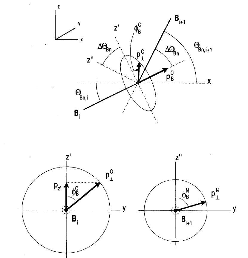
Figure 4: Figure 14 from Ellison, Baring, & Jones (1996) showing the geometry at the shock where the magnetic field changes direction and magnitude. In the notation used here $\Theta_{\mathrm{Bn},i}=\theta_{\mathrm{B0}}$, $\Theta_{\mathrm{Bn},i+1}=\theta_{\mathrm{B2}}$, $B_{i}=B_{0}$, and $B_{i+1}=B_{2}$.

2.3.2 Lorentz transformations and shock crossings

When a particle crosses the shock (where the bulk flow and magnetic field change direction and magnitude) its pitch angle and phase change discontinuously. However, until a scattering occurs, it moves smoothly and the magnitude of its momentum remains constant in a given reference frame. The details of the shock crossing are given in Ellison, Baring, & Jones (1996) and we reproduce Fig. 14 from that paper here as our Fig. 4. While the geometry described in Ellison, Baring, & Jones (1996) is identical to that used here, there are important differences in the techniques we now employ. The two most important differences are first, that our calculation is now fully relativistic and applies for all $\gamma_{0}$ and second, we no longer transform to the de Hoffmann-Teller (H-T) frame when crossing the shock. Before discussing the H-T frame, we describe (following the arguments in Ellison, Baring, & Jones, 1996) the calculations required in a shock crossing. For convenience of discussion we describe a particle crossing from upstream to downstream, although everything we present applies equally to particles crossing in either direction.

Having determined that a particle has crossed the shock, we first transform its local frame momentum (in this case, its momentum measured in the upstream frame, subscript “0”) to the shock frame:

$$p_{x,\mathrm{sk}} = \left[(\gamma_{u0}-1)\left(\frac{u_{x0}}{u_{0}}\right)^{2}+1\right]p_{x0}+$$

$$(\gamma_{u0}-1)\frac{u_{x0}u_{z0}}{u_{0}^{2}}p_{z0}+$$

$$\gamma_{u0}\gamma_{\mathrm{pf}}m_{p}u_{x0}\ ,$$

$$p_{y,\mathrm{sk}} = p_{y0}\ ,$$ (9)

$$p_{z,\mathrm{sk}} = (\gamma_{u0}-1)\left(\frac{u_{x0}u_{z0}}{u_{0}^{2}}\right)p_{x0}+$$ (10)

$$\left[(\gamma_{u0}-1)\left(\frac{u_{z0}}{u_{0}}\right)^{2}+1\right]p_{z0}+$$

$$\gamma_{u0}\gamma_{\mathrm{pf}}m_{p}u_{z0}\ .$$

Here, $\gamma_{u0}=[1-(u_{0}/c)^{2}]^{-1/2}$. Given the shock frame momentum, we now perform a transformation to the downstream frame. Note that the values of $u_{x}$, $u_{z}$, and $\gamma_{u}$ change to the downstream values for this transformation:

$$p_{x2} = \left[(\gamma_{u2}-1)\left(\frac{u_{x2}}{u_{2}}\right)^{2}+1\right]p_{x,\mathrm{sk}}+$$

$$(\gamma_{u2}-1)\left(\frac{u_{x2}u_{z2}}{u_{2}^{2}}\right)p_{z,\mathrm{sk}}-$$

$$\gamma_{u2}\gamma_{\mathrm{sk}}m_{p}u_{x2}\ ,$$

$$p_{y2} = p_{y,\mathrm{sk}}\ ,$$ (12)

$$p_{z2} = (\gamma_{u2}-1)\left(\frac{u_{x2}u_{z2}}{u_{2}^{2}}\right)p_{x,\mathrm{sk}}+$$ (13)

$$\left[(\gamma_{u2}-1)\left(\frac{u_{z2}}{u_{2}}\right)^{2}+1\right]p_{z,\mathrm{sk}}-$$

$$\gamma_{u2}\gamma_{\mathrm{sk}}m_{p}u_{z2}\ ,$$

where

$$\gamma_{\mathrm{sk}}=\sqrt{[p_{t,\mathrm{sk}}/(m_{p}c)]^{2}+1}$$ (14)

and

$$p_{t,\mathrm{sk}}=\sqrt{p_{x,\mathrm{sk}}^{2}+p_{y,\mathrm{sk}}^{2}+p_{z,\mathrm{sk}}^{2}}\ .$$ (15)

Simultaneously with these transformations, the new phase and pitch angle of the particle relative to the downstream magnetic field must be computed from the old phase and pitch angle measured against the upstream magnetic field. This is described in Fig. 4 where, in our current notation, $\Theta_{\mathrm{Bn},i}=\theta_{\mathrm{B0}}$, $\Theta_{\mathrm{Bn},i+1}=\theta_{\mathrm{B2}}$, $B_{i}=B_{0}$, and $B_{i+1}=B_{2}$, since we only consider unmodified shocks. Referring to Fig. 4, the component of the old momentum (i.e., the momentum before crossing the shock) in the $y$-direction is

$$p_{y}={p}_{\perp 0}\sin{\phi_{B}^{0}}\ ,$$ (16)

and the component along the $z^{\prime}$-direction is

$${p}_{z^{\prime}}={p}_{\perp 0}\cos{\phi_{B}^{0}}\ ,$$ (17)

where ${p}_{\perp 0}$ is the component of momentum (measured in the upstream frame) perpendicular to $B_{0}$, and $z^{\prime}$ is perpendicular to the $y$-$B_{0}$ plane. The component of momentum along the $z^{\prime\prime}$-direction (i.e., the axis perpendicular to the $y$-$B_{2}$ plane) is:

$${p}_{z^{\prime\prime}}={p}_{z^{\prime}}\cos{\Delta\Theta_{\mathrm{Bn}}}-{p}_{B0}\sin{\Delta\Theta_{\mathrm{Bn}}}\ ,$$ (18)

where $\Delta\Theta_{\mathrm{Bn}}=\theta_{\mathrm{B2}}-\theta_{\mathrm{B0}}$. The total momentum perpendicular to the new (i.e., downstream) magnetic field $B_{2}$ is

$${p}_{\perp N}=\sqrt{p_{y}^{2}+{p}_{z^{\prime\prime}}^{2}}\ .$$ (19)

Finally, the new phase around $B_{2}$ is given by

$$\phi_{B}^{N}=\arctan{\frac{p_{y}}{{p}_{z^{\prime\prime}}}}\ .$$ (20)

The two frame transformations and the pitch angle and phase transformations occur in the instant the particle crosses the shock between scatterings. The fact that we include in the transformations the changing magnetic field strength and direction and the changing flow speed and direction, fully takes into account the u $\times$ B electric field. No transformation to the H-T frame is required. Furthermore, there is no need to assume the conservation of magnetic moment when crossing the shock.

2.3.3 de Hoffmann-Teller frame transformations

The de Hoffmann-Teller frame is the frame where the u $\times$ B electric field is zero. For the geometry shown in Fig. 1, the H-T frame moves in the negative $z$-direction with speed $v_{\mathrm{HT}}=\gamma_{0}u_{0}\tan{\theta_{\mathrm{B0}}}$. As mentioned above, this frame has been used for oblique shocks, particularly with guiding center approximations, in attempts to simplify calculations of the energy change a particle experiences in crossing the shock (e.g., Ellison, Baring, & Jones, 1996; Meli & Quenby, 2003b). Viewed from the shock frame, it appears that particles drifting in the shock layer experience an energy change from the u $\times$ B field which is not included in normal DSA where particles gain energy by scattering between the converging upstream and downstream plasmas. However, as was evident in the original formulation of nonrelativistic DSA (e.g., Blandford & Ostriker, 1978), where it was shown that the power-law index was independent of $\theta_{\mathrm{B0}}$, shock drift acceleration must be part of DSA.

From a particle point of view, particles gyrating across an oblique shock can, depending on their pitch angle, gyrate back and forth several times before being convected downstream or reflected. The energy change that occurs in this gyration can be viewed as that obtained by the particle in the u $\times$ B electric field as it moves a distance larger than a gyroradius in the shock layer. However, since the u $\times$ B field is zero in the H-T frame and nothing fundamental changes with a simple frame transformation, the energy change must be caused by some effect which does not depend explicitly on the electric field. In fact, as particles gyrate in the shock layer they continually cross and re-cross the shock and receive repeated energy changes from the frame transformations in the converging upstream and downstream flows. As long as enough scattering occurs to maintain near isotropic distributions in all frames, this is just the standard DSA process and gives exactly the same result as obtained from explicitly including the u $\times$ B electric field.

For scatter-free propagation, shock-drift acceleration can be viewed as an independent mechanism. In principle, it is possible, depending on the pitch angle a particle has in the upstream region, for a particle to gain a large amount of energy as it gyrates in the shock layer (e.g., Decker, 1988). For some pitch angles, upstream particles can even gyrate into the shock layer and return upstream, all without scattering. While in principle it is possible for a particular particle to gain a large amount of energy in this fashion, the range in pitch angles that result in large energy gains is extremely small and only a small fraction of all particles gain energies much in excess of that from a single shock compression. Scatter-free propagation, even for nonrelativistic shocks, does not result in a canonical power law but depends strongly on $\theta_{\mathrm{B0}}$ and the energy of the injected particles. If elastic scattering is included, at any level as long as it is strong enough to drive the distributions to isotropy, the process reverts to standard DSA.

In nonrelativistic shocks, a H-T frame can be found unless $\theta_{\mathrm{B0}}\simeq 90^{\circ}$ and a H-T transformation may be useful in some applications. However, a H-T frame with speed $<c$ is excluded when $\tan{\theta_{\mathrm{B0}}}>c/(u_{0}\gamma_{0})$, making this technique essentially useless for ultra-relativistic, oblique shocks.

Fortunately, as we have described above (and shown in Ellison, Jones, & Baring, 1999), there is no need to transform to the H-T frame and the effects of the u $\times$ B electric field can be included in the particle translation. This allows us to model relativistic shocks of arbitrary obliquity.

2.3.4 Probability of return and distribution function

The particle spectrum produced by the Fermi mechanism comes about from the average energy gain per shock crossing combined with the probability that a particle will make some number of crossings. The energy gain per crossing is given by the Lorentz transformations discussed above. The number of crossings a particle makes on average before escaping from the shock, is determined by the probability that a particle, once downstream, will be able to scatter back upstream. This can be determined in the Monte Carlo code by simply following a particle as it moves in the downstream region and assuming, once it reaches some number of diffusion lengths downstream from the shock that it has a vanishing probability of diffusing back upstream. A more efficient way of doing this is described in Appendix A3 of Ellison, Baring, & Jones (1996). Once a particle becomes isotopic in the downstream frame, the probability of it returning to some point in the downstream flow is

$$P_{\mathrm{ret}}=\left(\frac{v_{p}-u_{x2}}{v_{p}+u_{x2}}\right)^{2}\ .$$ (21)

This expression is relativistically correct (e.g., Peacock, 1981) and applies for any shock obliquity.

For relativistic shocks, the distribution function $f(p)$ is calculated in the following way. As downstream particles leave the shock system, either from the probability of return test or from a set number of diffusion lengths downstream, they are binned in momentum space and $f(p)$ is formed using the shock-frame $p_{t,\mathrm{sk}}$. All of our distributions with $\gamma_{0}\geq 2$ are calculated this way.

We note that in our previous work (e.g., Jones & Ellison, 1991; Ellison & Double, 2002) we calculated the distribution at specific locations (i.e., specific $y-z$ planes) by summing $(p_{t,\mathrm{sk}}/|p_{x,\mathrm{sk}}|)$ each time a particle crossed the plane. This produces an omni-directional distribution and is useful for simulating what a detector will measure at a particular location relative to the shock. There is an implicit assumption of isotropy with this technique which can be satisfied for nonrelativistic shocks and, in nonrelativistic shocks, the omni-directional distribution and the one determined from particles leaving downstream are equivalent as long as the $y-z$ plane is well downstream and all particles are isotropic. For relativistic shocks, anisotropies persist and the two methods give somewhat different results depending on where the omni-directional flux is calculated.

Figure 5: Distribution functions, $f(p)$, versus momentum, $p$, for various input conditions as labeled. Note that we plot $p^{4}f(p)$ in the top panel and $p^{4.23}f(p)$ in the bottom. Spectra with the expected nonrelativistic, test-particle power-law index will be horizontal in this representation. The distributions are omni-directional and are calculated in the shock frame, downstream from the shock.

3 Results

3.1 Non-relativistic shocks

In Fig. 5 we show $f(p)$ versus $p$ for nonrelativistic shocks (i.e., $u_{0}=3000$ and $10^{4}$ km s^-1). The spectra are omni-directional measured downstream from the shock in the shock reference frame. The important features in these plots are:

(i) In the top panel, the distributions all become power laws with index $\sigma\simeq\sigma_{\mathrm{TP}}=3r/(r-1)\simeq 4$ when $v_{p}\gg u_{0}$. This confirms that our technique, which does not make a transformation to the H-T frame, properly accounts for the energy gain in the shock layer without explicitly including the u $\times$ B electric field. To emphasize this point, we show in the bottom panel the spectrum from a shock with a low Alfvén Mach number $M_{A}\simeq 4.6$. The parameters for this shock are: proton density $=1$ cm^-3, unshocked proton temperature $=10^{5}$ K, unshocked electron temperature $=10^{6}$ K, and $B_{0}=3\times 10^{-4}$ G. In this case, the magnetic field is strong enough to produce a significant change in downstream flow direction (i.e., $\theta_{\mathrm{u2}}\simeq 10.1^{\circ}$) and to modify the jump conditions giving a compression ratio of $r\simeq 3.43$. Here, we plot $p^{4.23}f(p)$, where $4.23=3r/(r-1)$, and the horizontal power law confirms that we get the correct $\sigma_{\mathrm{TP}}$. The dynamically important magnetic field makes this a stronger test of our translation technique than the cases in the top panel where $B_{0}=10^{-6}$ G. For the $\theta_{\mathrm{B0}}=60^{\circ}$ shocks in the top panel, the sonic Mach number $M_{S}\simeq 81$, $M_{A}\simeq 4600$ and $\theta_{\mathrm{u2}}\simeq 1.4\times 10^{-5}$ degrees.

(ii) The normalization of the power law relative to the thermal peak drops as either $\eta_{\mathrm{mfp}}$ or $\theta_{\mathrm{B0}}$ is increased. This drop occurs before particles become isotropic and comes about because particles with $v_{p}\not\gg u_{0}$ enter the downstream region directed predominantly along the shock normal. This makes it harder for them to scatter back upstream and the difficulty increases when either $\eta_{\mathrm{mfp}}$ or $\theta_{\mathrm{B0}}$ is large.

Particles gyrate around and along the magnetic field. In the absence of cross-field diffusion, the greater $\theta_{\mathrm{B2}}$, the further particles have to move along the field to move a given distance normal to the shock. This increases the likelihood that they will convect downstream without further acceleration. When $\eta_{\mathrm{mfp}}$ is large, cross-field diffusion is less important compared to scattering along the magnetic field and particles again are less likely to scatter back upstream.

Note that the probability of return equation (21), which does not include $\theta_{\mathrm{B2}}$, is still valid even though particles are swept downstream more quickly in oblique shocks than in parallel ones. As a downstream particle gyrates around the magnetic field, it will cross a particular point in the downstream flow more often if the field is oblique than if it is parallel. If this point is used to calculate $P_{\mathrm{ret}}$, the particle will have some probability of escaping every time it gyrates across this point and is more likely to escape downstream than would be the case in a parallel shock. Nevertheless, the test-particle power law index $\sigma_{\mathrm{TP}}$ is obtained once particles become isotropic since, on average, a particle gains more energy per shock crossing in an oblique shock than in a parallel one because it can gyrate across the shock several times in a single shock crossing event. These two effects, more energy per crossing but smaller probability of making $N$ crossings, each depend in the same way on $\theta_{\mathrm{B2}}$ or $\eta_{\mathrm{mfp}}$ for isotropic particles and combine to give the canonical $\sigma_{\mathrm{TP}}$ once $v_{p}\gg u_{0}$.

(iii) The minimum momentum where the power-law tail obtains increases with increasing $\theta_{\mathrm{B0}}$. This is particularly noticeable with the $\theta_{\mathrm{B0}}=89^{\circ}$ example in the top panel of Fig. 5 and comes about because, to obtain $\sigma_{\mathrm{TP}}$, particles must have a speed large compared to the effective flow speed. In oblique shocks, this speed is essentially the H-T velocity and the momentum where $\sigma_{\mathrm{TP}}$ is established increases with $\theta_{\mathrm{B0}}$.

The non-power-law tail coming off the thermal distribution in oblique shocks may be important in the heliosphere where highly oblique interplanetary traveling shocks accelerate the thermal solar wind (e.g., Baring et al., 1997). The energetic particles observed by spacecraft may not show the canonical Fermi power law even though DSA is the physical mechanism producing the energetic population.

Figure 6: Distribution functions, $f(p)$, versus momentum, $p$, for various input conditions as labeled. Note that we plot $p^{4.29}f(p)$, where $4.29\simeq 3r/(r-1)=\sigma_{\mathrm{TP}}$, i.e., the spectral index expected for nonrelativistic shocks with $r=3.32$. The light-weight solid curve in the top panel uses a small value of $N_{g}$. These are trans-relativistic shocks with $\gamma_{0}=2$ and show spectra both flatter and steeper than $\sigma_{\mathrm{TP}}$.

3.2 Trans-relativistic shocks

As soon as the flow speed becomes comparable to the speed of light, the power-law index starts to depend strongly on $\eta_{\mathrm{mfp}}$ and $\theta_{\mathrm{B0}}$. In Fig. 6 we show results for a trans-relativistic shock with $\gamma_{0}=2$ for various $\eta_{\mathrm{mfp}}$ and $\theta_{\mathrm{B0}}$. These shocks all have $r\simeq 3.32$ as determined by the jump conditions given in Double et al. (2004) and we plot $p^{4.29}f(p)$, where $4.29\simeq 3r/(r-1)$. The spectra are measured in the shock frame from escaping particles. In all cases except for the light-weight solid curve in the top panel, the value of $N_{g}$ is large enough to produce convergent results. The heavy-weight solid curve in the top panel is the parallel shock case and has $\sigma\simeq 4.1$. The other curves in the top panel show results with $\theta_{\mathrm{B0}}=60^{\circ}$ for various $\eta_{\mathrm{mfp}}$. A power law is obtained in each case, but there is a strong steepening of the power-law portion of the spectrum with increasing $\eta_{\mathrm{mfp}}$.

In the bottom panel of Fig. 6 we show the highly oblique case $\theta_{\mathrm{B0}}=89^{\circ}$ for various $\eta_{\mathrm{mfp}}$. The spectra are similar to those with $\theta_{\mathrm{B0}}=60^{\circ}$ except the steepening with increasing $\eta_{\mathrm{mfp}}$ is greater.

As $\gamma_{0}$ increases, the influence of $N_{g}$ increases, but it is still small for $\gamma_{0}=2$. The light-weight solid curve in the top panel of Fig. 6 was calculated with the same parameters as the dotted curve except that $N_{g}=20$ rather than 1200 for the dotted curve. The small $N_{g}$ produces a slight steepening of the power law.

Figure 7: Distribution functions, $f(p)$, versus momentum, $p$, for shocks with $\gamma_{0}=10$. Note that the canonical power law index for ultra-relativistic shocks is $\sigma\simeq 4.23$ and we plot $p^{4.23}f(p)$ to emphasize this result.

Figure 8: Distribution functions, $f(p)$, versus momentum, $p$, for shocks with $\gamma_{0}=20$ (top panel) and $\gamma_{0}=30$ (bottom panel). We plot $p^{4.23}f(p)$ to emphasize the $\theta_{\mathrm{B0}}=0^{\circ}$ result.

3.3 Fully relativistic shocks

In Fig. 7 we show results with $\gamma_{0}=10$ for various $\eta_{\mathrm{mfp}}$ and $\theta_{\mathrm{B0}}$. These shocks all have $r\simeq 3.02$ ($\sigma_{\mathrm{TP}}\simeq 4.49$) but we have plotted $p^{4.23}f(p)$, where $4.23$ is the index known to result for fully relativistic, parallel shocks with strong scattering (e.g., Ballard & Heavens, 1991; Bednarz & Ostrowski, 1998; Achterberg et al., 2001; Ellison & Double, 2002). In all cases, the value of $N_{g}$ is large enough to produce convergent results. The solid curve in the top panel confirms that we obtain the canonical result for $\theta_{\mathrm{B0}}=0^{\circ}$.

For $\theta_{\mathrm{B0}}>0^{\circ}$, the results show the same general trend as those for the trans-relativistic shocks in Fig. 6. The top panels of Figs. 6 and 7 are similar except the steepening for $\gamma_{0}=10$ is a less dramatic function of $\eta_{\mathrm{mfp}}$. The same is true for the bottom panels where $\theta_{\mathrm{B0}}=89^{\circ}$.

Figure 9: Distribution functions, $f(p)$, versus momentum, $p$, for shocks with $\gamma_{0}=20$. The parameter $N_{g}$ is varied while all other input parameters are held constant.

The computation time required to produce convergent results (i.e., results with large enough $N_{g}$) increases with $\gamma_{0}$ so we show a limited number of examples with $\gamma_{0}>10$. Fig. 8 shows results for $\gamma_{0}=20$ (top panel) and $\gamma_{0}=30$ (bottom panel) and these examples, combined with our $\gamma_{0}=10$ result, show a clear trend. First of all, the standard $\sigma\sim 4.23$ result for $\theta_{\mathrm{B0}}=0^{\circ}$ is obtained in all cases. For $\theta_{\mathrm{B0}}>0^{\circ}$, we get results very similar to those for $\gamma_{0}=10$ with a general reduction in the variation caused by varying $\theta_{\mathrm{B0}}$ or $\eta_{\mathrm{mfp}}$. It is likely that this trend will continue, supporting the assertion that ultra-relativistic shocks produce power laws with $\sigma\simeq 4.23$ independent of $\theta_{\mathrm{B0}}$ or $\eta_{\mathrm{mfp}}$. This assumes, of course, that $N_{g}$ is large enough to produce convergence.

The effect of varying $N_{g}$ when $\gamma_{0}=20$ and $\theta_{\mathrm{B0}}=0^{\circ}$ is shown in Fig. 9 (similar results are obtained for $\gamma_{0}=10$ and 30). This parameter now dramatically influences the spectrum. The step-function effect in the spectrum has been noted by several authors in the context of large-angle scattering (e.g., Quenby & Lieu, 1989; Ellison, Jones, & Reynolds, 1990; Baring, 1999) (see also Vietri, 1995). Fig. 9 shows that this effect emerges smoothly from the canonical $\sigma=4.23$ power law as $N_{g}$ is lowered and scattering becomes coarser. Notice that the momentum of the first peak above thermal energies depends on $N_{g}$. For $N_{g}=100$ this peak occurs at $\sim 10^{3}m_{p}c$ rather than $\gamma_{0}^{2}m_{p}c$ because the curves in Fig. 9 (and all others in this paper) are calculated in the shock frame. Plotted in the downstream plasma frame, this peak is at $\sim\gamma_{0}^{2}m_{p}c$ as expected.

Figure 10: Distribution functions with $\gamma_{0}=20$ for small $N_{g}=200$ and various $\theta_{\mathrm{B0}}$ and $\eta_{\mathrm{mfp}}$, as indicated.

In Fig. 10 we show the effect of coarse scattering (small $N_{g}=40$) as a function of $\eta_{\mathrm{mfp}}$ for $\gamma_{0}=20$ and $\theta_{\mathrm{B0}}=60^{\circ}$. The step-like structure remains as the spectra steepen with increasing $\eta_{\mathrm{mfp}}$, although the steps begin to smooth some.

Figure 11: Pitch-angle distributions for shock crossing particles in shocks ranging from nonrelativistic to fully relativistic, as indicated. A positive $p_{x,\mathrm{sk}}$ indicates motion toward the downstream direction. The area under each curve is normalized to one.

3.4 Pitch-angle distributions

The anisotropic nature of particles in relativistic shocks produces the strong dependencies we’ve seen on $\theta_{\mathrm{B0}}$, $\eta_{\mathrm{mfp}}$, and $N_{g}$. The main difference between nonrelativistic and relativistic shocks is shown in Fig. 11, where we compare the pitch-angle distributions of shock crossing particles. The curves are calculated by summing the quantity $p_{x,\mathrm{sk}}/p_{t,\mathrm{sk}}$ as particles cross the shock and only superthermal particles are included in the plots. These are shock-frame values of momentum and the dashed curve from our nonrelativistic example (Fig. 5) shows the flux weighting characteristic of an isotropic distribution, i.e., particles cross the shock with a frequency proportional to their component of velocity normal to the shock.

The relativistic shocks show highly anisotropic pitch-angle distributions with most particles crossing into the downstream region at an oblique angle. For a given set of parameters $\gamma_{0}$, $\theta_{\mathrm{B0}}$, $\eta_{\mathrm{mfp}}$, and $N_{g}$, a particular pitch-angle distribution results and this determines the average momentum gain in a shock crossing. This combined with the probability to make some number of crossings determines the spectrum. Unlike for nonrelativistic shocks with their isotopic distributions, no simple analytic expression has been found for $\sigma$ once flows become trans-relativistic.

Figure 12: Pitch-angle distributions for the shocks shown in Fig. 7. The area under each curve is normalized to one.

In Fig. 12 we show the pitch-angle distributions for the examples shown in Fig. 7. It’s clear that relatively subtle changes in the pitch-angle distribution causes fairly large changes in $f(p)$. The bottom panel for $\theta_{\mathrm{B0}}=89^{\circ}$ shows the trend as $\eta_{\mathrm{mfp}}$ increases; the larger $\eta_{\mathrm{mfp}}$, the more peaked the distribution is at $p_{x,\mathrm{sk}}/p_{t,\mathrm{sk}}\sim 0.6$ with a smaller fraction of particles crossing back into the upstream region.

Figure 13: Pitch-angle distributions for shocks with parameters similar to those in Fig. 9. The area under each curve is normalized to one.

Finally, in Fig. 13 we show pitch-angle distributions as $N_{g}$ is varied as in Fig. 9. When $N_{g}$ is small, the pitch-angle distribution is strongly peaked in the forward direction and this is responsible for the step-like nature of $f(p)$. As $N_{g}$ is increased, the distribution smoothly moves to a configuration similar to those shown in Fig. 12.

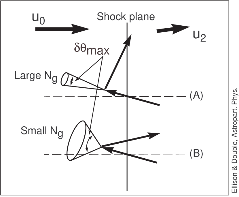
Figure 14: Schematic representation of particles crossing a shock with large and small values of $N_{g}$.

We illustrate this in Fig. 14. When $v_{p}\not\gg u_{0}$, flux weighting causes most particles crossing into the upstream region from downstream to be directed close to the shock normal, i.e., with pitch angles near $180^{\circ}$. A large $N_{g}$ means a particle will interact after a short $\delta t$ with a small $\delta\theta_{\rm max}$ and is less likely to broaden its pitch angle much before being swept back across the shock. This is illustrated in Fig. 14 with the particle trajectory labeled (A). If $N_{g}$ is small, $\delta\theta_{\rm max}$ is larger, the particle changes its pitch angle by a larger amount on average, and there is a greater chance the particle will cross back into the downstream region with a flatter trajectory as shown with the trajectory labeled (B). On average, particles crossing as in (A) with a large $N_{g}$ receive less energy per crossing than those crossing as in (B), where $N_{g}$ is small.

4 Conclusions

We have presented a comprehensive study of test-particle, diffusive shock acceleration in plane shocks of varying Lorentz factor $\gamma_{0}$, obliquity $\theta_{\mathrm{B0}}$, and scattering properties parameterized by $\eta_{\mathrm{mfp}}$ and $N_{g}$. We use a Monte Carlo computer simulation which smoothly spans the parameter space from nonrelativistic shocks through trans-relativistic ones to fully relativistic shocks, without requiring a transformation to the de Hoffmann-Teller frame or making any assumptions concerning the magnetic moment of shock crossing particles. Due to the Lorentz transformation of the magnetic field, relativistic shocks will have superluminal H-T speeds for virtually all obliquities, making transformations to the H-T frame of limited use.

For nonrelativistic shock speeds, the test-particle Fermi power law has a well-known analytic form which is used to test our computer simulations. For trans-relativistic and fully relativistic shocks, however, analytic results are rare or non-existent although several independent calculations provide a canonical power-law for ultra-relativistic particles in parallel, ultra-relativistic shocks, i.e., $f(p)\propto p^{-4.23\pm 0.1}$. We obtain this result and the fact that our simulation has a single algorithmic sequence spanning all $\gamma_{0}$’s and $\theta_{\mathrm{B0}}$’s provides some measure of assurance that our results are accurate in trans-relativistic regions where analytical results do not exist.

In contrast to nonrelativistic shocks, DSA in relativistic shocks depends critically on the details of how particles interact with the background magnetic turbulence. In real shocks, this turbulence must be self generated by the shock accelerated particles. However, the scattering interactions responsible for this generation are not known with any reliability and particle diffusion must be parameterized. Despite the complexity and unknown nature of the wave-particle interactions, we believe that much of the essential underlying physics can be modeled by first assuming that the scattering mean free path $\lambda$ is proportional to the gyroradius $r_{g}$ and then defining two parameters which control the finer scattering details. These parameters are $\eta_{\mathrm{mfp}}$ in the relation $\lambda=\eta_{\mathrm{mfp}}r_{g}$, which characterizes the “strength” of cross-field scattering, and the “fineness” of pitch-angle scattering $N_{g}$, where particles pitch-angle scatter after a fraction of a gyro-period $\delta t=\tau_{g}/N_{g}$ within a maximum angle given by eqn. (4). Spectra converge to a particular form as $N_{g}$ increases and the convergent value of $N_{g}$ is proportional to $\gamma_{0}^{2}$.

Our results show that particle distributions depend strongly on $\eta_{\mathrm{mfp}}$ and $\theta_{\mathrm{B0}}$, as well as on $N_{g}$ for relativistic shocks when $N_{g}$ is below the convergent value. Most importantly, we show that $f(p)$ departs significantly from $f(p)\propto p^{-4.23}$ in a wide trans-relativistic regime extending to above $\gamma_{0}=30$.

In our examples with $\gamma_{0}=2$ we find that the power law is flatter than $\sigma_{\mathrm{TP}}=3r/(r-1)$ (Fig. 6) for $\theta_{\mathrm{B0}}=0^{\circ}$. That is, the power-law index $\sigma\simeq 4.12$ versus $\sigma_{\mathrm{TP}}\simeq 4.29$. As long as $\theta_{\mathrm{B0}}=0^{\circ}$, the results are independent of $\eta_{\mathrm{mfp}}$. For $\theta_{\mathrm{B0}}>0^{\circ}$, the power law steepens as either $\theta_{\mathrm{B0}}$ or $\eta_{\mathrm{mfp}}$ is increased. For our most extreme $\gamma_{0}=2$ case, $\theta_{\mathrm{B0}}=89^{\circ}$ and $\eta_{\mathrm{mfp}}=6$, yielding $\sigma\simeq 6.5$.

For our more strongly relativistic examples ($\gamma_{0}\geq 10$), with convergence values of $N_{g}$, we obtain the canonical power-law index $\sigma\simeq 4.23$ for $\theta_{\mathrm{B0}}=0^{\circ}$. As with $\gamma_{0}=2$, the power law steepens when either $\theta_{\mathrm{B0}}$ or $\eta_{\mathrm{mfp}}$ is increased (Figs. 7 and 8), but the steepening becomes a weaker function of both $\theta_{\mathrm{B0}}$ and $\eta_{\mathrm{mfp}}$ as $\gamma_{0}$ increases. Our results are consistent with $\sigma\rightarrow 4.23$ independently of $\theta_{\mathrm{B0}}$ and $\eta_{\mathrm{mfp}}$ in the ultra-relativistic limit as widely reported (e.g., Bednarz & Ostrowski, 1998; Achterberg et al., 2001). We do show, however, that a wide range of Lorentz factors exists extending up to $\gamma_{0}\sim 30$ where $\sigma$ differs significantly from $4.23$.

In contrast to the effects of $\theta_{\mathrm{B0}}$ and $\eta_{\mathrm{mfp}}$, which diminish with increasing $\gamma_{0}$, the influence of $N_{g}$ remains as $\gamma_{0}$ increases. Figs. 9 and 10 show that small $N_{g}$ (large-angle scattering) produces large features in the spectra as individual shock crossings continue to show in $f(p)$ to high energies. There is no reason to believe this effect will diminish with increasing $\gamma_{0}$.

It is not at all obvious what realistic values of $N_{g}$ are or if they are large enough to produce convergence. Large values of $N_{g}$ imply that significant power in magnetic turbulence exists at extremely small length scales and it is possible that actual plasmas have some lower length-scale limit which may be larger than needed for convergence. In this case, the spectrum will depend on the effective $N_{g}$ and may be highly variable depending on the particle shock parameters. Furthermore, the highest momentum particles require magnetic turbulence with extremely long length scales for resonance. If this turbulence does not exist, the spectrum will turn over at some characteristic momentum determined by the longest magnetic length scale (see Niemiec & Ostrowski, 2004, for a discussion of such effects).

Some of the most exotic and interesting astrophysical objects are likely to harbor relativistic shocks. While it is probable that these shocks accelerate particles, the spectrum, even in unmodified, ultra-relativistic shocks, depends on the unknown details of the wave-particle interactions.

References

- Achterberg et al. (2001) Achterberg, A., Gallant, Y. A., Kirk, J. G., & Guthmann, A. W., 2001, MNRAS, 328, 393
- Axford, Leer, & Skadron (1977) Axford, W. I., Leer, E., & Skadron, G., 1977, in Proc. 15th ICRC (Plovdiv), 11, 132
- Ballard & Heavens (1991) Ballard, K.R. & Heavens, A.F., 1991, MNRAS, 251, 438
- Baring (1999) Baring, M. G. 1999, Proc. 26th Int. Cosmic Ray Conf. (Salt Lake City), 4, 5
- Baring et al. (1997) Baring, M. G., Ogilvie, K. W., Ellison, D. C., Forsyth, R. J., 1997, ApJ, 476, 889
- Bednarz & Ostrowski (1996) Bednarz, J. & Ostrowski, M., 1996, MNRAS, 283, 447
- Bednarz & Ostrowski (1998) Bednarz, J. & Ostrowski, M., 1998, Phys. Rev. Letts, 80, 3911
- Bell (1978) Bell, A. R., 1978, MNRAS, 182, 147
- Blandford & Ostriker (1978) Blandford, R.D., & Ostriker, J.P., 1978, ApJ, 221, L29
- Decker (1988) Decker, R. B., 1988, Space Sci. Rev., 48, 195
- Double (2003) Double, G. P. “Investigation of Lepton and Baryon Acceleration in Relativistic Astrophysical Shocks,” 2003, PhD Thesis, North Carolina State University, Raleigh, North Carolina
- Double et al. (2004) Double, G. P., Baring, M. G., Jones, F. C., & Ellison, D. C., 2004, ApJ, 600, 485
- Ellison, Baring, & Jones (1995) Ellison, D. C., Baring, M. G., & Jones, F. C., 1995, ApJ, 453, 873
- Ellison, Baring, & Jones (1996) Ellison, D. C., Baring, M. G., & Jones, F. C., 1996, ApJ, 473, 1029
- Ellison & Double (2002) Ellison, D. C. & Double, G. P., 2002, Astropart. Phys., 18, 213
- Ellison, Jones, & Baring (1999) Ellison, D. C., Jones, F. C., & Baring, M. G., 1999, ApJ, 512, 403
- Ellison, Jones, & Reynolds (1990) Ellison, D. C., Reynolds, S. P., & Jones, F. C., 1990, ApJ, 360, 702
- Ellison, Möbius, & Paschmann (1990) Ellison, D. C., Möbius, E., & Paschmann, G., 1990, ApJ, 352, 376
- Heavens & Drury (1988) Heavens, A.F. & Drury, L. O’C., 1988, MNRAS, 235, 997
- Jones & Ellison (1991) Jones, F.C., & Ellison, D.C., 1991, Space Sci. Rev., 58, 259
- Kirk & Heavens (1989) Kirk, J.G. & Heavens, A.F., 1989, MNRAS, 239, 995
- Kirk & Schneider (1987) Kirk, J.G. & Schneider, P., 1987, ApJ, 322, 256
- Krymsky (1977) Krymsky, G. F. 1977, Soviet Phys. Dokl., 22, 327.
- Meli (2002) Meli, A., “Particle Acceleration at Relativistic and Ultra-Relativistic Shock Waves”, 2002, PhD Thesis, Imperial College London, University of London
- Meli & Quenby (2003a) Meli, A. and Quenby, J. J., 2003b, Astropart. Phys., 19, 637
- Meli & Quenby (2003b) Meli, A. and Quenby, J. J., 2003b, Astropart. Phys., 19, 649
- Niemiec & Ostrowski (2004) Niemiec, J., & Ostrowski, M., 2004, in press (astro-ph/0401397)
- Ostrowski (1991) Ostrowski, M., 1991, MNRAS, 249, 551
- Ostrowski (1993) Ostrowski, M., 1993, MNRAS, 264, 248
- Peacock (1981) Peacock, J. A., 1981, MNRAS, 196, 135
- Piran (1999) Piran, T., 1999, Phys. Repts., 314, 575
- Quenby & Lieu (1989) Quenby, J. J., & Lieu, R., 1989, Nature, 342, 654
- Rees (2000) Rees, M.J., 2000, Nuclear Phys. A, 663, 42
- Vietri (1995) Vietri, M., 1995, ApJ, 453, 883
- Waxman (2000) Waxman, E., 1900, ApJS, 127, 519