Fe II/Mg II EMISSION LINE RATIOS OF QSOs. II. $z>6$ OBJECTS

Abstract

Near-infrared spectra of four QSOs located at $z>6$ are obtained with the OH-airglow suppressor mounted on the Subaru telescope. The Fe II/Mg II emission-line ratios of these QSOs are examined by the same fitting algorithm as in our previous study of $z<5.3$ QSOs. The fitting results show that two out of the four $z>6$ QSOs have significant Fe II emission in their rest-UV spectra, while the other two have almost no Fe II features. We also applied our fitting algorithm to more than 10,000 SDSS QSOs and found two trends in the distribution of Fe II/Mg II against redshift: (1) the upper envelope of the Fe II/Mg II distribution at $z>3$ shows a probable declination toward high redshift, and (2) the median distribution settles into lower ratios at $z\sim 1.5$ with small scatter compared to the other redshift. We discuss an Fe/Mg abundance evolution of QSOs with a substantial contribution from the diverse nature of the broad-line regions in high-redshift QSOs.

1 INTRODUCTION

The Fe/Mg abundance ratio, one of the most important parameters for estimating the age of a stellar system after its initial starburst, is based on the delay of iron enrichment by Type Ia supernovae and compared with the formation of such $\alpha$-elements as magnesium by Type II supernovae (see Hamann & Ferland 1999 for a review). The delay of iron formation was generally thought to be $\sim 1$ Gyr (e.g., Yoshii et al. 1996), while more recent studies suggest that this delay can be $\sim 0.3$ Gyr, depending on environmental conditions of the star formation process (Friaca & Terlevich, 1998; Matteucci & Recchi, 2001). The Fe II(UV)/Mg II emission-line ratio of QSOs is considered a probable indicator of the Fe/Mg abundance ratio, which has been measured in various redshift ranges: $3.1<z<4.7$ by Thompson et al. (1999, hereafter THE99), $0<z<5.3$ by Iwamuro et al. (2002, hereafter Paper I), $5.7<z<6.3$ by Freudling et al. (2003), $0<z<4.8$ by Dietrich et al. (2003), and $3.0<z<6.4$ by Maiolino et al. (2003). The median values of the Fe II/Mg II emission-line ratios are almost constant at all redshifts, while large scatter dominates the distribution of the ratios at $z>3$, indicating the diversity of the formation histories of high-redshift QSOs. On the other hand, recent photoionization calculations of Fe⁺ atoms in the broad-line regions of QSOs show that the Fe II(UV)/Mg II emission-line ratio is sensitive not only to Fe and Mg abundance but also to physical conditions, including microturbulence (Verner et al., 2003). However, the median value of the Fe II/Mg II emission-line ratio is expected to converge on a significantly smaller value when the age of the universe becomes less than $\sim 0.3$ – 1 Gyr, assuming that the substantial scatter caused by the diverse characteristics (or microturbulence velocities, etc.) of the broad-line regions in QSOs has the same contribution at any redshift.

In this paper, we report the Fe II/Mg II emission-line ratios of four QSOs at $z>6$ observed by the OH-airglow suppressor (OHS; Iwamuro et al. 2001) and CISCO (Motohara et al., 2002) mounted on the Subaru telescope. In $\S 2$ we analyze the data by the same method as in Paper I, and then we compare the results with other observations in $\S 3$. In $\S 4$ we discuss the expected Fe/Mg abundance evolution of QSOs using the combined samples of these results, the new Sloan Digital Sky Survey (SDSS) archival data, and the previous samples in Paper I. Throughout the paper we adopt a cosmology with $H_{0}=70$ km s^-1 Mpc^-1, $\Omega_{M}=0.3$, and $\Omega_{\Lambda}=0.7$.

2 OBSERVATIONS AND DATA REDUCTION

The observations were carried out on 2002 February 27 and March 2 and again on 2003 March 20 and 21, using OHS and CISCO mounted on the Subaru telescope. Since the Fe II and Mg II are redshifted to the $H$ and $K$ bands, respectively, for $z>6$ QSOs, the $K$-band spectra were obtained by CISCO and the $JH$-band spectra by OHS separately in each observation run. The typical exposure sequence is 200 s $\times$ 3 $\times$ 4 positions (CISCO) or 1000 s $\times$ 4 positions (OHS), in which the object is moved about $10\arcsec$ along the slit by nodding the telescope after every three exposures (CISCO) or one exposure (OHS). The slit widths were $0\farcs 8$ (CISCO) and $1\arcsec$ (OHS), providing spectral resolutions of 330 and 210, respectively. After this exposure sequence, a nearby SAO star with a spectral type of A or F was observed as a spectroscopic standard to remove the telluric atmosphere absorption features and to correct the instrumental response. The pixel scale was $0\farcs 106$/pixel with the infrared secondary mirror of the telescope, while the seeing size was $0\farcs 7$. To calibrate the relative flux between the $K$- and $JH$-band spectra, short imaging exposures of 20 s $\times$ 3 $\times$ 4 positions were executed by CISCO in both the $K^{\prime}$ (1.97–2.30 $\mu$m) and $H$ (1.50–1.79 $\mu$m) bands, except for SDSS 1030+0524. The observation log is summarized in Table 1.

The obtained data were reduced using IRAF with typical reduction procedures for infrared images (see Paper I). The resultant one-dimensional spectra in the $K$ and $JH$ bands were combined using the photometric results of the imaging observation by CISCO. As a result, through a circular aperture of 2$\farcs$2 diameter, the average fluxes between 1.97–2.30 and 1.50–1.79 $\mu$m correspond to the $K^{\prime}$- and $H$-band magnitudes respectively. The extraction procedure for Fe II and Mg II emission lines from the combined spectra is the same as in Paper I: nonlinear $\chi^{2}$ fitting for the Mg II (Moffat function) and for the continuum (power law) profile with six free parameters, after subtraction of the Fe II template from the composite QSO spectrum of the Large Bright Quasar Survey (LBQS; Francis et al. 1991) and the Balmer continuum template from the UV spectrum of 3C 273 (Wills et al., 1985) with various multiplying factors (see eq. (1)–(4) in Paper I). The fitting range is 2150–3300Å, which is also the wavelength range for our definition of Fe II flux. Note that the strength of the Fe II emission is determined by shape comparison between our Fe II template and the observed spectral features (large bumps and small depressions), which does not require the assumption of the power-law continuum level (we need the assumption of the shape of the Fe II template instead).

Although the Moffat function is very useful for fitting the various profiles of Mg II emission lines with the minimum number of parameters, a serious problem is that the fitted Mg II profile sometimes has very broad wings. To prevent such unexpected broad wings, we set the lower limits at $b\geq 0.5$ for the Moffat power (eq. (1) in Paper I) and reanalyzed all the data fitted with $b<0.5$ in Paper I (see Appendix).

3 RESULTS

The object spectra with fitted components are shown in Figure 1, and the numerical results are listed in Table 2. The spectra with wavelengths longer than 1.80 $\mu$m are obtained by CISCO, and the shorter parts by OHS. The strength of the Fe II emission is mainly determined by the break feature at rest 2200Å, which is observed by OHS with superior signal-to-noise ratios. The wavelength range between 1.80 and 1.95 $\mu$m corresponds to the atmospheric absorption band, whose contribution to the fitting results is very small because of large errors.

As shown in Figure 1 and Table 2, we detected strong Fe II emission from SDSS J1148+5251, which is consistent with Maiolino et al. (2003). SDSS J1048+4637 also shows significant Fe II emission, while the Fe II/Mg II ratio is not as much as the value of $\sim$8.1 reported by Maiolino et al. (2003). The absorption-line feature at 1.29 $\mu$m in SDSS J1048+4637 is the broad absorption line component of C III] reported by Maiolino et al. (2004). The observed spectra of these objects fit well into our template spectrum of Fe II in every detail. Although Barth et al. (2003) reported a smaller Fe II/Mg II ratio of $\sim$4.7 for SDSS J1148+5251, this inconsistency is mostly caused by the difference in the Fe II template under Mg II emission. On the other hand, SDSS J1030+0524 and SDSS J1630+4012 show almost no Fe II emission or any break feature at rest 2200Å. These results for SDSS J1030+0524 are consistent with Freudling et al.(2003), as well as the unknown absorption-line feature at 1.57 $\mu$m. As a result, even at $z>6$, the Fe II(UV)/Mg II emission-line ratios still show large diversity.

4 DISCUSSION

Figure 2 shows the Fe II/Mg II ratio and the absolute AB magnitude at rest 2500Å as a function of redshift, for which we reanalyzed the SDSS data on the basis of the DR1 quasar catalog (Schneider et al., 2003). The other $z<5.3$ data are the same as those plotted in Figure 7 of Paper I, except for four objects listed in the Appendix. The median values and the standard deviation of the sample distribution are shown by the squares with the cross bars in this figure whose numerical values are listed in Table 3. Although the number of samples at $z>3$ is insufficient to make a statistical argument, we can deduce the trends of the evolution of the Fe II/Mg II ratio from Figure 2. First, the median Fe II/Mg II ratios at $z>3$ are almost constant, while the upper envelope of the distribution plotted by the dashed line in Figure 2 shows a probable declination toward high redshift. Second, the median distribution settles into lower ratios at $z\sim 1.5$, with small scatter compared to the other redshift. Here, the downward error bars from these median points are almost equal to the typical fitting errors of the samples in each bin (column 3 in Table 3), while the longer upward error bars are affected by the substantial scatter of the Fe II/Mg II ratios.

Assuming that the Fe/Mg abundance ratio affects these rough trends, these small Fe II/Mg II ratios at $z\sim 1.5$ originated with the dilution of the Fe abundance with the outflow gas from low-mass stars after $\sim$3 Gyr from the initial starburst (Yoshii et al., 1998). The scatter of the sample at this redshift (a factor of $\sim$2 between the top and bottom of the cross bars) corresponds to the maximum contribution of the scatter caused by the differences in the physical conditions of the broad-line regions in high-redshift QSOs (Verner et al., 2003). If this substantial scatter of factor of $\sim$2 is the universal nature of the QSOs, independent of the redshift, the larger scatter of the $z>3$ samples are affected by the difference in the Fe/Mg abundance ratio or the time passage after the initial starburst. This idea is also consistent with the declination of the upper envelope of the Fe II/Mg II distribution toward high redshift, which is expected to be the initial abundance evolution of QSOs.

An alternative explanation for the variation of the Fe II/Mg II ratios at $z\sim 2$ may be their luminosity dependence such that the QSOs of higher luminosities, in a low-redshift ($z=$0.1-0.6) sample from Hubble Space Telescope ($HST$) UV archives (Tsuzuki, 2004) as well as in a high-redshift ($z=$3-5) sample from near-infrared observations (Iwamuro et al., 2002; Dietrich et al., 2003), are found to have higher Fe II/Mg II ratios. The larger variation of the Fe II/Mg II ratios for the brighter QSOs suggests that either the ionizing photon flux arriving at the broad-line-emitting clouds or the physical characteristics of the clouds would scatter more significantly for brighter QSOs. To estimate their respective contributions to the Fe II/Mg II ratio is a theoretical challenge that requires an elaborate photoionization model of Fe⁺ in the broad-line regions of QSOs.

Appendix A Re-analyzed Objects Having Broad Mg II Wings

We re-analyzed all the data having broad Mg II wings ($b<0.5$) in Paper I with lower limits at $b\geq 0.5$ for the Moffat profile of

$$F_{MgII}(\lambda)=i\left[1+\left(\frac{\lambda-2798\AA}{a}\right)^{2}\right]^{-b}.$$ (A1)

All the data were fitted with $b=0.5$ (Lorentzian), and the results are listed in Table 4. Three out of seven objects listed in Table 4 are not plotted in Figure 2 because we adopted the results of the OHS data rather than those of THE99 and the results of the $HST$ FOS archive rather than those of Kinney et al. (1991) (see Table 2 and Table 4 in Paper I).

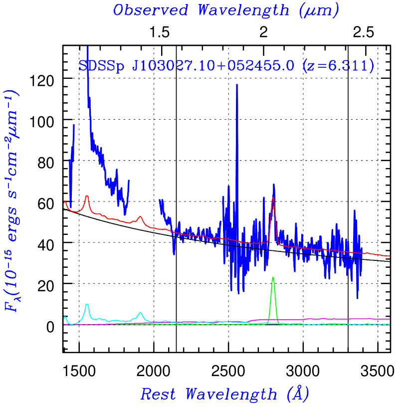
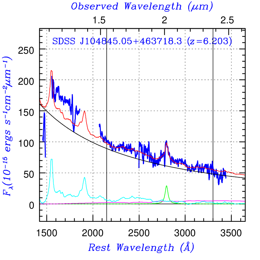
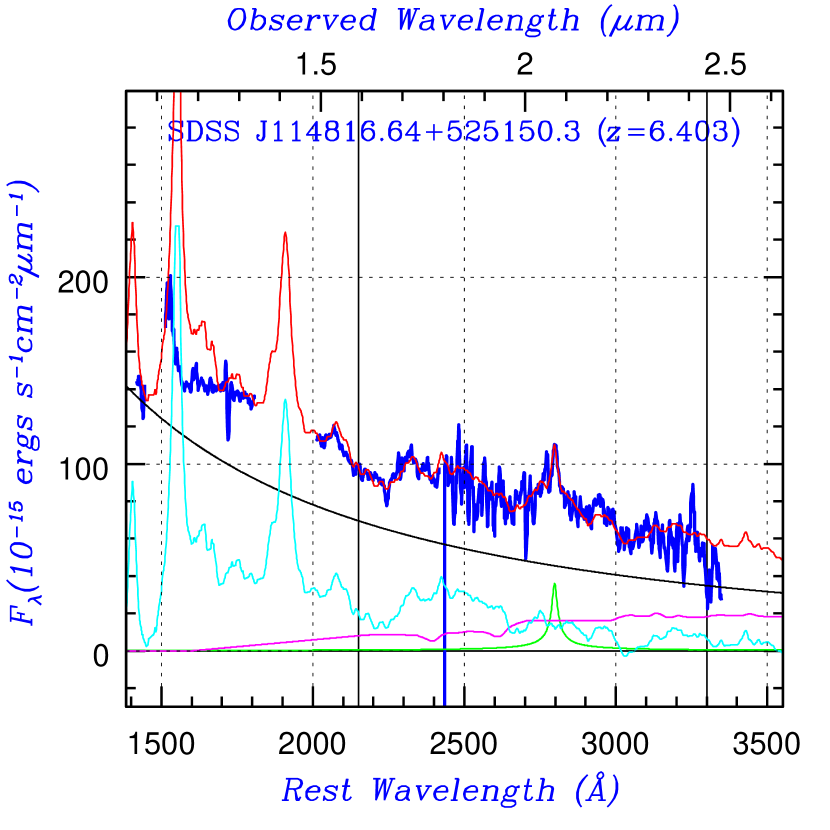
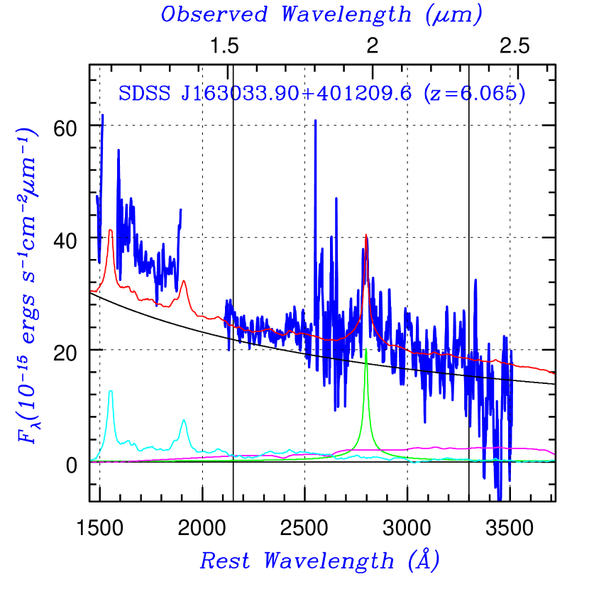
Figure 1: Observed spectra of the four QSOs listed in Table 1. A power law continuum, Mg II, Fe II, a Balmer continuum (including other lines except for Mg II), and the sum of these components are plotted for comparison with the observed spectrum with the boxcar-smoothing of six pixels. The two vertical lines indicate the fitting range of 2150–3300Å in the rest-wavelength.

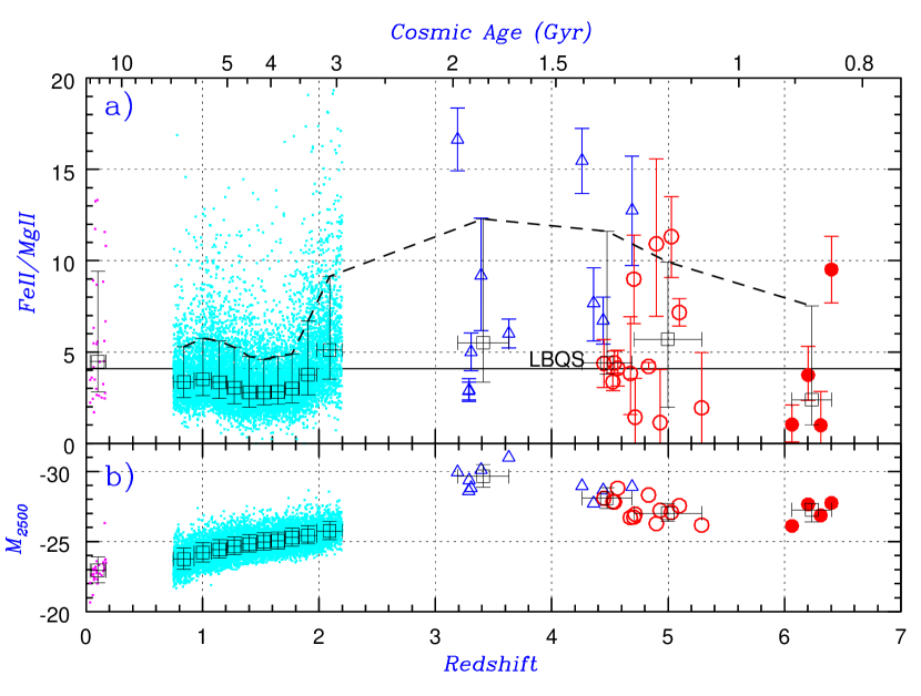
Figure 2: Redshifts vs. Fe II/Mg II and absolute magnitudes. The fitting results for the QSO spectra from Kinney et al. (1991), $HST$/FOS and SDSS archives (dots), THE99 (triangles), our data in Paper I (open circles), and this work (filled circles) are plotted with the median values (squares) of the appropriate bins. The horizontal solid line indicates the Fe II/Mg II of 4.09 for the LBQS composite spectrum (see Paper I). The squares with the cross-bars represent the median values and the standard deviations of the sample distribution, whose upper envelope is connected by a broken line. We assume $H_{0}=70$ km s^-1 Mpc^-1, $\Omega_{M}=0.3$, and $\Omega_{\Lambda}=0.7$ for the estimation of $M_{2500}$ (the absolute AB-magnitude at rest-frame 2500Å) and the cosmic age at the redshift.

Table 1: Log of Observations

						Exposure		Coordinate
Object Name	Redshift	$K^{\prime}$-mag	$H$-mag	Date	Instrument	Time (s)	Seeing	Reference
SDSS J103027.10+052455.0 (catalog )	6.28	17.67	—	2002 Feb.27	CISCO	2400	0$\farcs$80	1
		—	18.57	2002 Mar. 2	OHS	4000	0$\farcs$88
SDSS J104845.05+463718.3 (catalog )	6.23	17.12	17.76	2003 Mar.20	CISCO	2400	0$\farcs$56	2
		—	17.83	2003 Mar.21	OHS	4000	0$\farcs$71
SDSS J114816.64+525150.3 (catalog )	6.43	16.98	17.70	2003 Mar.20	CISCO	2400	0$\farcs$65	2
		—	17.62	2003 Mar.21	OHS	4000	0$\farcs$62
SDSS J163033.90+401209.6 (catalog )	6.05	18.40	19.25	2003 Mar.20	CISCO	2400	0$\farcs$71	2
		—	19.18	2003 Mar.21	OHS	8000	0$\farcs$68

References. — (1) Fan et al. (2001); (2) Fan et al. (2003).

Table 2: Results of Fitting Calculations

		FWHM	$I$(Fe II)	$I$(Mg II)		$EW$(Fe II)	$EW$(Mg II)
Object Name	$z$	(km s-1)	(10-16ergs s-1cm-2)		Fe II/Mg II	(Å)	(Å)
SDSS J103027.10+052455.0 (catalog )	6.311	3590	5.96${}^{+11.1}_{-5.96}$	6.04$\pm$1.40	0.99${}^{+1.86}_{-0.99}$	21.0	22.9
SDSS J104845.05+463718.3 (catalog )	6.203	4050	42.4$\pm$14.7	11.3$\pm$2.1	3.74$\pm$1.47	81.8	25.7
SDSS J114816.64+525150.3 (catalog )	6.403	3020	137$\pm$16	14.4$\pm$2.2	9.52$\pm$1.82	333	41.7
SDSS J163033.90+401209.6 (catalog )	6.065	2690	7.30$\pm$7.00	7.12$\pm$1.61	1.02$\pm$1.01	52.2	55.8

Table 3: Median values of Fe II/Mg II

Redshift	Fe II/Mg II	Error	Number
0.101$\pm$0.068	4.48${}^{+4.95}_{-1.66}$	0.84	30
0.839$\pm$0.089	3.36${}^{+1.93}_{-0.85}$	0.82	1101
1.003$\pm$0.075	3.49${}^{+2.26}_{-0.89}$	0.90	1101
1.144$\pm$0.066	3.34${}^{+2.25}_{-0.88}$	0.90	1101
1.273$\pm$0.063	3.05${}^{+2.22}_{-0.89}$	0.92	1101
1.402$\pm$0.066	2.78${}^{+1.98}_{-0.81}$	0.93	1101
1.528$\pm$0.060	2.79${}^{+1.80}_{-0.70}$	0.81	1101
1.647$\pm$0.060	2.81${}^{+1.94}_{-0.67}$	0.84	1101
1.769$\pm$0.063	3.00${}^{+1.89}_{-0.81}$	0.95	1101
1.907$\pm$0.075	3.75${}^{+2.95}_{-1.10}$	1.24	1101
2.091$\pm$0.109	5.11${}^{+4.03}_{-1.60}$	1.67	1099
3.411$\pm$0.220	5.50${}^{+6.77}_{-2.16}$	1.45	6
4.475$\pm$0.215	4.40${}^{+7.22}_{-0.61}$	1.76	9
4.997$\pm$0.291	5.69${}^{+4.25}_{-3.71}$	2.70	8
6.234$\pm$0.169	2.38${}^{+5.14}_{-1.37}$	2.02	4

Table 4: Results of Fitting Calculations for THE99 data

		FWHM		$EW$(Fe II)	$EW$(Mg II)
Object Name	$z$	(km s-1)	Fe II/Mg II	(Å)	(Å)	Reference
BR 1033$-$0327 (catalog )	4.527	4050	2.34$\pm$0.78	98.5	46.6	THE99
1358+391 (catalog )	3.288	4610	2.86$\pm$0.49	110	46.1	THE99
PKS 2126$-$158 (catalog )	3.290	3430	2.92$\pm$0.63	71.3	29.1	THE99
IIIZw 2 (catalog )	0.089	3020	1.95$\pm$0.28	155	79.1	$IUE$
PG 0844+349 (catalog )	0.065	2320	6.31$\pm$0.23	238	40.4	$HST$
IRAS 1334+24 (catalog )	0.109	3010	2.62$\pm$0.27	138	40.9	$HST$
MRC 2251-178 (catalog )	0.064	4200	3.53$\pm$0.27	424	143	$IUE$

References. — ($IUE$) Kinney et al. (1991) (ftp://dbc.nao.ac.jp/DBC/NASAADC/catalogs/3/3157/); ($HST$) $HST$ archive in CADC (http://cadcwww.dao.nrc.ca/hst/science.html); (THE99) Thompson et al. (1999)

References

- Barth et al. (2003) Barth, A. J., Martini, P., Nelson, C. H., & Ho, L. C. 2003, ApJ, 594, L95
- Dietrich et al. (2003) Dietrich, M., Hamann, F., Appenzeller, I., & Vestergaard, M. 2003, ApJ, 596, 817
- Fan et al. (2001) Fan, X. et al. 2001, AJ, 122, 2833
- Fan et al. (2003) Fan, X. et al. 2003, AJ, 125, 1649
- Francis et al. (1991) Francis, P. J., Hewett, P. C., Foltz, C. B., Chaffee, F. H., Weymann, R. J., & Morris, S. L. 1991, ApJ, 373, 465
- Freudling et al. (2003) Freudling, W., Corbin, M. R., & Korista, K. T. 2003, ApJ, 587, L67
- Friaca & Terlevich (1998) Friaca, A. C. S. & Terlevich, R. J. 1998, MNRAS, 298, 399
- Hamann & Ferland (1999) Hamann, F. & Ferland, G. 1999, ARA&A, 37, 487
- Iwamuro et al. (2001) Iwamuro, F., Motohara, K., Maihara, T., Hata, R., & Harashima, T. 2001, PASJ, 53, 355
- Iwamuro et al. (2002) Iwamuro, F., Motohara, K., Maihara, T., Kimura, M., Yoshii, Y., & Doi, M. 2002, ApJ, 565, 63
- Kinney et al. (1991) Kinney, A. L., Bohlin, R. C., Blades, J. C., & York, D. G. 1991, ApJS, 75, 645
- Maiolino et al. (2003) Maiolino, R., Juarez, Y., Mujica, R., Nagar, N. M., & Oliva, E. 2003, ApJ, 596, L155
- Maiolino et al. (2004) Maiolino, R., Oliva, E., Ghinassi, F., Pedani, M., Mannucci, F., Mujica, R., & Juarez, Y. 2003, A&A submitted, (astro-ph/0312402)
- Matteucci & Recchi (2001) Matteucci, F. & Recchi, S. 2001, ApJ, 558, 351
- Motohara et al. (2002) Motohara, K. et al. 2002, PASJ, 54, 315
- Schneider et al. (2003) Schneider, D. P. et al. 2003, AJ, 126, 2579
- Thompson et al. (1999) Thompson, K. L., Hill, G. J., & Elston, R. 1999, ApJ, 515, 487
- Tsuzuki (2004) Tsuzuki, Y. 2004, Ph.D. thesis, University of Tokyo
- Verner et al. (2003) Verner, E., Bruhweiler, F., Verner, D., Johansson, S., & Gull, T. 2003, ApJ, 592, L59
- Wills et al. (1985) Wills, B. J., Netzer, H., & Wills, D. 1985, ApJ, 288, 94
- Yoshii et al. (1996) Yoshii, Y., Tsujimoto, T., & Nomoto, K. 1996, ApJ, 462, 266
- Yoshii et al. (1998) Yoshii, Y., Tsujimoto, T., & Kawara, K. 1998, ApJ, 507, L113