Electric field screening by a proton counterflow in the pulsar polar cap

We propose a new mechanism to screen the electric field in the pulsar polar cap. Previous studies have shown that if an electron beam from the stellar surface is accelerated to energies high enough to create electron-positron pairs, the required electric field parallel to the magnetic field lines is too strong to be screened out by the produced pairs. We argue here that if non-relativistic protons are supplied from the magnetosphere to flow towards the stellar surface, they can provide an anode to screen out such a strong electric field. Injected electron-positron pairs yield an asymmetry of the electrostatic potential around the screening point. The required pair creation rate in this model is consistent with the conventional models.

1 INTRODUCTION

A spinning magnetized neutron star provides huge electric potential differences between different parts of its surface as a result of unipolar induction (Goldreich & Julian, 1969). A part of the potential difference may be expended on an electric field along the magnetic field somewhere in the magnetosphere. Although a fully self-consistent model for the pulsar magnetosphere has not yet been constructed, several promising models have been proposed. Among them, the polar cap model (Sturrock, 1971; Ruderman & Sutherland, 1975) assumes that an electric field $E_{\parallel}$ parallel to the magnetic field lines exists just above the magnetic poles. The electric field accelerates charged particles up to TeV energies, and resultant curvature radiation from these particles produces copious electron-positron pairs through magnetic pair production. These pairs may be sources for gamma-ray emission, coherent radio emission, and the pulsar wind.

The localized potential drop is maintained by a pair of anode and cathode regions. In the cathode region the space charge density $\rho$ deviates from the Goldreich-Julian (GJ) density negatively. On the other hand, $\rho$ must deviate positively for the anode. Outside the accelerator the electric field will be screened. In the polar cap model, especially for a space charge-limited flow model (Fawley et al., 1977; Scharlemann et al., 1978; Arons & Scharlemann, 1979), where electrons can freely escape from the stellar surface, i.e., $E_{\parallel}=0$ on the stellar surface, the formation mechanism of a static anode-cathode pair that can sustain enough potential drop for pair production is a long-standing issue. Since the current flows steadily along the magnetic field lines, the charge density is determined by the magnitude of the current and the field geometry with suitable boundary conditions. Basic considerations on this problem for space charge-limited flows are given in Shibata (1997). The mechanism of the electric field screening, i.e., a way to provide an anode, may be provided by pair polarization. Although most papers take it for granted that copious pair production can instantly screen the field, recently Shibata et al. (1998, 2002: hereafter SMT98 and SMT02, respectively) have casted doubt on this issue; electric field screening is not as easy as most researchers consider conventionally.

SMT98 and SMT02 investigated the screening of electric fields in the pair production region. They found that the required thickness of the screening layer is restricted to be as small as the braking distance $l_{\rm E}=m_{\rm e}c^{2}/|eE_{\parallel}|$, for which decelerating particles become non-relativistic, where $m_{\rm e}$ and $-e$ are the electron mass and charge, respectively. If the above condition does not hold, too many positrons are reflected back and destroy the negative charge region (cathode). In order to screen the electric field consistently, a huge number of pairs should be injected within a region as small as $l_{\rm E}$. The required pair multiplication factor per primary particle is enormously large and cannot be realized in the conventional pair creation models. Thus, some other ingredients are required for the electric field screening.

In relation to this problem, Lyubarskii (1992) proposed a model with a positron counterflow and argued that the model makes it possible to screen the electric field for any current density. He showed that the electric field on the stellar surface can be screened by the injection of electron-positron pairs plus a positron counterflow from the magnetosphere for any current density. In his model the positron counterflow is introduced to adjust the current desnity in the polar cap and does not play a critical role as an anode formation. Most importantly, his model is different from the space charge-limited flow considered here and cannot be applied to our problem. As SMT98 and SMT02 have shown, the way to screen the electric field at a reasonable altitude is unknown for space charge-limited flows which we believe to be the most suitable model because the work function of the matter on the neutron surface is considered to be small enough.

In previous studies of the screening, pairs were assumed to accelerate or decelerate along the 0-th order trajectories determined by $E_{\parallel}$. However, if an electrostatic (longitudinal) instability occurs, the excited waves may produce effective friction which will change the charge polarization process. Asano & Takahara (2004) numerically investigated an electrostatic instability of electron-positron pairs injected in an external electric field. However, they found that the density of electron-positron pairs in the standard pulsar model is too low to induce the instability needed to provide strong friction. This means that each particle moves stably along the trajectory determined by the external electric field since collective forces from other particles are negligible.

In this paper, we present a new model with a proton counterflow to solve the screening problem in the polar cap model with pair injection. Since the proton mass is much larger than the electron mass, its inertia effect is much stronger and can provide an anode structure more easily if non-relativistic protons are supplied from the outer magnetosphere to flow towards the polar caps. Our purpose is to point out a possibility that the proton flow can explain the structure of the electric field in the polar cap. Therefore, our model is highly idealized and simplified. Detailed investigations of the situation in our model are beyond the scope of the present paper. In Sect. 2 we briefly summarize the space charge-limited flow model in the pulsar polar cap to give a basic framework for the present model. In Sect. 3 we consider the model with proton counterflow and demonstrate the effectiveness of the screening by the proton counterflow. Sect. 4 is devoted to a summary and discussion.

2 THE POTENTIAL FOR SPACE CHARGE LIMITED FLOW

Before we present the model with a proton counterflow, we summarize the basic features of the behaviour of the electric potential in the pulsar polar cap to make clear the fundamental points of the problem. The notations are the same as in SMT98 and SMT02 in which the one-dimensional (1D) approximation is used. We assume that $\mathbf{\Omega}_{*}\cdot\mathbf{B}>0$, where $\mathbf{\Omega}_{*}$ and $\mathbf{B}$ are the angular velocity of the star and magnetic field, respectively. Although the current density distribution is most likely to be determined by the global dynamics in the magnetosphere, we will investigate a local region just above the stellar pole. We therefore treat the current density as an adjustable free parameter in our paper, as assumed in SMT98 and SMT02. A steady electron beam flows from the stellar surface and is accelerated by a negative electric field parallel to a magnetic field line with zero electric field on the stellar surface. Beyond a certain altitude called the pair production front (PPF), electron-positron pairs are assumed to be injected continuously into space. In this case a part of the injected positrons returns towards the stellar surface. Here, we consider mainly the behavior of the electric potential inside the PPF while that outside the PPF was treated in SMT02.

Since the current due to the primary electron beam flowing outward and that due to positrons returning towards the stellar surface flow inward along the magnetic field, both currents are negative. Inside the PPF the difference in the charge density determined by these currents and the GJ density gives the effective charge density. We define the GJ current density as

$$J_{0}\equiv-\frac{\mathbf{\Omega}_{*}\cdot\mathbf{B}}{2\pi}.$$ (1)

We normalize the potential $\Phi$, length along the magnetic field line $s$, GJ current density $J_{0}$, current density due to the primary electron beam $J$, and current density due to the returning positrons $J_{+}$ as

$$\phi \equiv \frac{e\Phi}{m_{\rm e}c^{2}},$$ (2)

$$l \equiv \frac{\omega_{\rm p}s}{c},$$ (3)

$$j_{0} \equiv \frac{J_{0}}{J_{B}},$$ (4)

$$j \equiv \frac{J}{J_{B}},$$ (5)

$$j_{+} \equiv \frac{J_{+}}{J_{B}},$$ (6)

where

$$J_{B} \equiv -\frac{\Omega_{*}B}{2\pi}<0,$$ (7)

$$\omega_{\rm p}^{2} \equiv \frac{4\pi e|J_{B}|}{m_{\rm e}c}.$$ (8)

The current densities $J$, $J_{+}$, $J_{0}$, and $J_{B}$ are all negative, so that $j_{0}$, $j$, $j_{+}$ are all positive, and by definition $j_{0}\leq 1$. The equation of continuity ensures that $j\propto J/B$ and $j_{+}\propto J_{+}/B$ are constant along the magnetic field line. On the other hand, $j_{0}\propto B_{z}/B$, where $B_{z}$ is the component of the magnetic field along the rotation axis, may change along the field line. When the magnetic field line curves away from the rotation axis, $j_{0}$ decreases with increasing $l$. Conversely, when the field line curves toward the rotation axis, $j_{0}$ increases with $l$. Adopting the 1D approximation, the non-dimensional Poisson equation becomes

$$\frac{d^{2}\phi}{dl^{2}}=\frac{j}{\beta}+\frac{j_{+}}{\beta_{+}}-j_{0}\simeq\frac{j}{\beta}-j_{+}-j_{0},$$ (9)

where $\beta=v/c>0$ and $\beta_{+}=v_{+}/c<0$ are velocities of the primary electron beam and the returning positrons normalized by the light velocity, respectively. Since positrons are ultra-relativistic inside the PPF, we have approximated as $\beta_{+}\simeq-1$ here.

The boundary conditions are given on the stellar surface ($l=0$) as follows; $\phi=0$, $d\phi/dl=0$, and the electron beam is supplied with $\beta=0$. In this case, the first term due to the electron beam, on the right hand side of Eq. (9), dominates the other terms on the stellar surface. The non-relativistic electron beam provides a huge negative charge density at $l=0$. As a result, just above the stellar surface $d^{2}\phi/dl^{2}>0$, which means that the potential curve is downward convex, irrespective of $j_{+}$ and $j_{0}$. As long as the first term $j/\beta$ dominates, $\phi$ increases with increasing $l$ and the electric field becomes negative. The electric field accelerates the electron beam, and $\beta$ becomes $\simeq 1$ at a certain altitude. Hereafter, we represent the scale of the transition from $\beta\sim 0$ to $\sim 1$ as $l_{\rm nr}$; for $l>l_{\rm nr}$, we write $\beta\simeq 1$. For $l>l_{\rm nr}$, the Poisson equation is approximated as

$$\frac{d^{2}\phi}{dl^{2}}=-\rho_{\rm in},$$ (10)

where

$$\rho_{\rm in}\equiv-j+j_{+}+j_{0},$$ (11)

is the effective charge density inside the PPF except for $0<l<l_{\rm nr}$. In general, the scale $l_{\rm nr}$ is much smaller than the length from the stellar surface to the PPF. In the greater part inside the PPF, the potential obeys Eq. (10).

When we assume that $j_{0}$ is constant neglecting effects of field line curvature, $\rho_{\rm in}$ is constant. In this case, the behaviour of the potential is determined only by $\rho_{\rm in}$ and the situation is classified into the two cases: $\rho_{\rm in}<0$ and $\rho_{\rm in}>0$. Hereafter we call the case of $\rho_{\rm in}<0$ ($j>j_{+}+j_{0}$) Super-GJ and that of $\rho_{\rm in}>0$ ($j<j_{+}+j_{0}$) Sub-GJ.

2.1 Sub-GJ

First, we discuss Sub-GJ. In the region inside $l_{\rm nr}$, the non-dimensional electric field $E=-d\phi/dl<0$ grows with $l$ as was mentioned before. For Sub-GJ, $d^{2}\phi/dl^{2}$ for $l>l_{\rm nr}$ is negative, so that the potential curve is upward convex. In this region the absolute value of $E$ declines with $l$ as schematically shown in Fig. 1. The electric field can be screened at a certain distance even without pair formation. In the approximation of constant $\rho_{\rm in}$, the solution of Eq. (10) is obtained as

$$\phi = -\frac{\rho_{\rm in}}{2}l^{2}+E_{0}l,$$ (12)

$$E = -\frac{d\phi}{dl}=-E_{0}+\rho_{\rm in}l,$$ (13)

where $E_{0}>0$ represents the magnitude of the electric field at $l=0$. Strictly speaking, for $l<l_{\rm nr}$ the above solution is not correct and the electric field grows from 0 at $l=0$ to $-E_{0}$ inside $l_{\rm nr}$. The length $l_{\rm nr}$ is negligibly small when considering the region $l>l_{\rm nr}$. From Eq. (13), the screening altitude, where the electric field becomes zero again, is approximated as

$$l_{\rm scr}=\frac{E_{0}}{\rho_{\rm in}}.$$ (14)

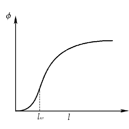
Figure 1: Potential for Sub-GJ and constant $j_{0}$. The position $l=l_{\rm nr}$ is the inflection point. For $l<l_{\rm nr}$, the effective charge density is negative, owing to the non-relativistic electron beam. For $l>l_{\rm nr}$, the effective charge density becomes $\rho_{\rm in}>0$.

If there is no pair injection, the electric field is not screened but changes sign at $l_{\rm scr}$ so that the electrons are decelerated outside $l_{\rm scr}$. Thus, the model becomes inconsistent. Let us further assume that around $l_{\rm scr}$ electron-positron pairs are injected and the electric field is screened. We represent the Lorentz factor of the beam at $l=l_{\rm scr}$ as $\Gamma(=\phi(l_{\rm scr})+1)=10^{6}\Gamma_{6}$. Using $\Gamma$, the electric field at $l=0$ is written by

$$E_{0}\simeq\sqrt{2\rho_{\rm in}\Gamma}.$$ (15)

Substituting this into Eq. (14), the altitude of the screening is obtained as

$$s_{\rm scr} = \frac{cl_{\rm scr}}{\omega_{\rm p}}=\sqrt{\frac{2\Gamma}{\rho_{\rm in}}}\frac{c}{\omega_{\rm p}},$$ (16)

$$= 5\times 10^{4}\Gamma_{6}^{1/2}\rho_{{\rm in},-3}^{-1/2}T_{0.3}^{1/2}B_{12}^{-1/2}\quad{\rm cm},$$ (17)

where $\rho_{{\rm in},-3}=\rho_{\rm in}/10^{-3}$, $B_{12}=B/10^{12}$ G and $T=0.3T_{0.3}$ s is the rotation period of pulsar.

To estimate $l_{\rm scr}$, we must estimate plausible ranges of $E_{0}$, $\rho_{\rm in}$ and $\Gamma$. The value of $\Gamma$ is considered to be $10^{6}\sim 10^{7}$ to obtain copious pair production. To constrain $E_{0}$ and $\rho_{\rm in}$, let us consider the behaviour of the potential just above the stellar surface ($l<l_{\rm nr}$). Multiplying Eq. (9) by $E$ and integrating it from the stellar surface to an arbitrary height,

$$-\frac{1}{2}\left[E^{2}\right]_{l=0}^{l=l}=\int_{0}^{\phi}d\phi\left(j_{0}-\frac{j}{\beta}+j_{+}\right),$$ (18)

where we use the relation $Edl=-d\phi$. The above condition corresponds to the Gauss law; the column charge density between $l$ and the stellar surface is equal to $E(l)$. Then we obtain

$$-\frac{1}{2}E^{2}=(j_{0}+j_{+})\phi-j\sqrt{\phi^{2}+2\phi}.$$ (19)

For Sub-GJ, $|E|$ takes the maximum value at $\phi=\phi_{\rm m}$ which is given by

$$\phi_{\rm m}^{2}+2\phi_{\rm m}=\frac{A^{2}}{1-A^{2}},$$ (20)

where $A\equiv j/(j_{0}+j_{+})<1$. From Eq. (19), we obtain the maximum electric field as

$$\frac{1}{2}E_{\rm max}^{2}=(1-\sqrt{\mathstrut 1-A^{2}})(j_{0}+j_{+})<j_{0}+j_{+},$$ (21)

We consider that this electric field gives an estimate of $E_{0}$ in Eq. (15). Then we have

$$\Gamma\simeq\frac{E_{\rm max}^{2}}{2\rho_{\rm in}}<\frac{j_{0}+j_{+}}{\rho_{\rm in}}.$$ (22)

Since $\Gamma$ is very large, $\rho_{\rm in}$ should be very small as long as $j_{0}$ and $j_{+}$ are of order of unity.

In order to complete the electric field screening, the effective charge density should be zero outside $l_{\rm scr}$ which is identified with the PPF. Outside the PPF, excess pair electrons provide the normalized current $j_{-}$ which is equal to the current $j_{+}$ due to returning positrons inside the PPF. Using the approximation that both electrons and positrons are relativistic, the effective charge density outside the PPF is given by

$$\rho_{\rm out}\equiv-j-j_{+}+j_{0}=0.$$ (23)

Thus, $j_{+}=j_{0}-j$ should be satisfied for self-consistency. The value $j_{+}$ to be positive requires $j<j_{0}$, which is equivalent to the Sub-GJ condition without pair injection. Then the constraint of a very small $\rho_{\rm in}=2(j_{0}-j)=2j_{+}$ implies that the number of returning positrons is very small and that $E_{0}$ is of order of unity (see Eq. (21)). If we assume $\Gamma\sim 10^{6}$, $\rho_{\rm in}\sim 10^{-6}$, which implies a high screening height of $s_{\rm scr}\sim 10^{6}$ cm from Eq. (17). This altitude is much higher than conventionally supposed and actually, geometrical effects will play a role either in screening or in changing the flow into a Super-GJ flow.

2.2 Super-GJ

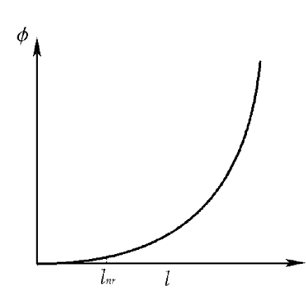
Figure 2: Potential for Super-GJ and constant $j_{0}$. The effective charge density is negative everywhere independently of the velocity of the electron beam.

For Super-GJ, since $\rho_{\rm in}<0$ and $d^{2}\phi/dl^{2}>0$ the potential curve is downward convex everywhere (see Fig. 2), The potential and the amplitude of the electric field steadily increase with $l$. The electric field is given by Eq. (13) and becomes

$$E\simeq\rho_{\rm in}l,$$ (24)

for large $l$ by neglecting $E_{0}$. If we conventionally assume that pair production can screen the electric field and if we also assume that the screening height $l_{\rm scr}$ roughly corresponds to the PPF, the screening height turns out to be given by Eq. (17), when $\rho_{\rm in}$ is replaced by $|\rho_{\rm in}|$. The non-dimensional electric field around the PPF is obtained as

$$E_{\rm scr}\simeq-\sqrt{2|\rho_{\rm in}|\Gamma}=-44.7\times|\rho_{{\rm in},-3}|^{1/2}\Gamma_{6}^{1/2}.$$ (25)

If $|\rho_{\rm in}|$ is large, $E_{\rm scr}$ becomes large around the PPF, while the screening height becomes low. As was shown in SMT02, pair polarization cannot screen the field when $E_{\rm scr}$ is more than a few. If $E_{\rm scr}$ is lower than a few, the situation is the same as for Sub-GJ, i.e., geometrical effects play a role without pair production. Another problem of Super-GJ is the following. For Super-GJ, the condition that the effective charge density outside the PPF vanishes becomes

$$\rho_{\rm out}=-j-j_{+}+j_{0}=\rho_{\rm in}-2j_{+}=0,$$ (26)

where all the components are assumed to be relativistic. This condition is never satisfied for positive $j_{+}$ within the 1D approximation. In order to achieve screening for Super-GJ, some components should be non-relativistic. The existence of the anode implies that the effective charge is positive at the point where $E=0$. Therefore the effective charge density should decrease outside this point. As a result, the models may require that a space charge density wave continues outside the PPF as was shown in SMT98. In this wave, the speeds of electrons and positrons go and return repeatedly between a non-relativistic speed and the light speed. The average effective charge density outside of the PPF is zero, while the local charge density oscillates spatially.

3 THE PROTON COUNTERFLOW MODEL

Our proton counterflow model is motivated by the difficulties discussed in the previous section and provides a mechanism for realizing relevant $E_{\rm scr}$ and $l_{\rm scr}$ for a reasonable $\Gamma$. As was shown in SMT98 and SMT02 and discussed in the previous section, it is difficult to screen the electric field in the system composed of the electron beam and injected pairs only. For Super-GJ, we need to screen an electric field that is as strong as given by Eq. (25). In this section we show that non-relativistic protons flowing backward can screen the electric field owing to the large proton mass.

3.1 Origin of the Proton Counterflow

To resolve the screening problem, we add a proton counterflow as a minimal alteration to the standard model. The existence and origin of the proton counterflow is highly speculative and it is difficult to give definite mechanisms at the present stage. Although it is highly unlikely that protons flow towards the polar cap from outside the light cylinder, the proton counterflow can be realized if protons exist in the magnetosphere. Considering that we still do not well understand the fundamental issues of pulsar physics such as the current closure problem, we should be free from any kind of prejudices.

There are some candidates for the origin of the proton counterflow. One of the most plausible candidates for the source is protons existing in the co-rotating magnetosphere. In the 0-th approximation such protons are confined to closed magnetic lines so that the protons do not flow into the polar cap region. However, if transport phenomena like the anomalous diffusion found in laboratory plasmas occur, the protons can flow into the polar cap region across magnetic field lines. Electrostatic (longitudinal) drift-waves are considered to be the most dominant diffusion process in tokamaks (Liewer, 1985), while vast amounts of theoretical efforts have been devoted to the understanding of the anomalous diffusion.

A density gradient of particles is likely to exist on the boundary between open and closed field lines. The drift motion due to the density gradient occurs along the direction (hereafter $y$-axis) perpendicular to both field lines and the density gradient ($x$-axis). Electrostatic drift-waves are excited accompanying the drift motion, so that the induced electric field along the $y$-axis induces $\mathbf{E}\times\mathbf{B}$ drift and particles diffuse along the $x$-axis, which will provide the source of the proton counterflow. The diffusion coefficient for this process may be obtained from numerical simulations.

The source of the anomalous diffusion is not limited to the electrostatic drift-waves due to the density gradient. The extremely high brightness temperature of pulsar radio emission requires a coherent source for this radiation and excitation of strong plasma waves in the open field line region. These waves may affect the corotating magnetosphere to induce proton diffusion.

As an example, let us roughly estimate the amount of protons that diffuse from the co-rotating magnetosphere. Assuming that the diffusion occurs around the “outer region” (radius $R_{\rm O}\sim R_{\rm L}/2$, where $R_{\rm L}\equiv c/\Omega_{*}$ is the radius of the light cylinder). Since the magnetic field is relatively weak (typically $10^{3}$-$10^{6}$ G), the drift velocity $v_{\bot}\sim cE/B$ due to the excited electric field can be large enough. Here, we assume that the scale of the proton diffusion region $\Delta R$ is much smaller than $R_{\rm O}$. We denote $\Delta R=fR_{\rm O}$ ($f\ll 1$) hereafter. Then, the number of protons escaping from the co-rotating magnetosphere is written as

$$2\pi R_{\rm O}\Delta R\delta n_{\rm O}v_{\bot}=\pi f(c/\Omega_{*})^{2}\delta n_{\rm O}v_{\bot}/2,$$ (27)

where $\delta n_{\rm O}$ is the proton number density resonating with the excited waves.

As will be shown below, our model requires that the proton current density on the polar cap is of the order of the GJ-current density. The typical size of the polar cap region $R_{\rm pol}$ on the stellar surface is $\sim 10^{4}$ cm. In our model the number of protons flowing into the polar cap region per unit time is

$$\dot{N}_{\rm p}\sim\frac{J_{0}}{e}R_{\rm pol}^{2}\sim\frac{\Omega_{*}B_{*}R_{\rm pol}^{2}}{2\pi e},$$ (28)

where $B_{*}$ is the magnetic field on the stellar pole. The supply rate given by Eq. (27) is larger than the required rate if

$$\delta n_{\rm O} > \frac{B_{*}R_{\rm pol}^{2}\Omega_{*}^{3}}{\pi^{2}c^{2}efv_{\bot}}$$ (30)

$$\sim 700\times$$

$$T_{0.3}^{-3}B_{12}\left(\frac{R_{\rm pol}}{10^{4}{\rm cm}}\right)^{2}\left(\frac{f}{0.1}\right)^{-1}\left(\frac{v_{\bot}}{0.1c}\right)^{-1}{\rm cm^{-3}}.$$

This value seems very small for the atmosphere around such a high density celestial object, and it is less than the Goldreich-Julian density at $R_{\rm O}$, though there are large uncertainties for $v_{\bot}$ and $f$. In some atmosphere models (Ho & Lai, 2001; Zane et al., 2001) that are consistent with observed proton-cyclotron resonance in a soft gamma repeater or an anomalous X-ray pulsar (Ibrahim et al., 2003; Rea et al., 2003), the proton density is assumed to be larger than $10^{20}{\rm cm^{-3}}$. Although the situation here is quite different from such models, the proton density in the magnetosphere may be much higher than the value of Eq. (30). Therefore, we consider that it is not so unlikely that a fraction of the protons diffuse from the co-rotating magnetosphere flow into the polar cap region, and that the global dynamics in the magnetosphere adjusts the current density distribution to screen the electric field.

Further detailed discussion of the diffusion depends on the wave excitation mechanism, the model of global current flows, the model of the atmosphere, and the convection in the co-rotating magnetosphere etc., which are not well understood. We will not discuss those problems in this paper. There may be mechanisms for the diffusion from the co-rotating magnetosphere other than described here and we do not stick to a specific mechanism. The existence of protons may be connect with the current closure problem and the source and role of proton flows are interesting subjects in connection with all the problems in pulsar physics.

3.2 Overview of the Model

The schematic picture for the proton counterflow model is depicted in Fig. 3. As shown in this figure, our model incorporates a bulge of the potential, which is divided into the following four regions: region I ($E<0$, effective charge density $\rho_{\rm eff}<0$), II ($E<0$, $\rho_{\rm eff}>0$), III ($E>0$, $\rho_{\rm eff}>0$), and IV ($E>0$, $\rho_{\rm eff}<0$). The potential increases from the stellar surface through regions I and II and peaks at the boundary between regions II and III. At the peak of the potential the electric field becomes zero. Then the potential decreases and the electric field becomes positive in regions III and IV. Our model requires that the electric field vanishes again in region IV. The potential curve in region IV is downwards convex and reaches the bottom again (we call this point “valley”, hereafter). In our model we assume that pair electrons do not return, so that the potential drop should be smaller than the electron energy at injection. As was mentioned in Sect. 2.2, the potential continues to oscillate outside of the valley. The potential curve shown in Fig. 3 is possible if the proton counterflow exists, as will be explained below.

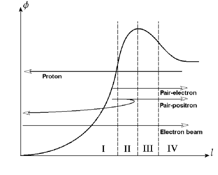
Figure 3: Schematic picture for the proton counterflow model.

We assume that the PPF is located in region I or II. Positrons in regions I and II are decelerated, and a part of the positrons returns towards the stellar surface. Therefore, in most of region I there are three relativistic flows: the electron beam coming from the stellar surface, the returning positron flow, and the proton counterflow. In this region the effective charge density determined from these flows is assumed to be negative (Super-GJ). As is discussed in Sect. 2.2, the amplitudes of the potential and electric field grow with $l$ in region I. As the potential increases with $l$, protons become non-relativistic and their speed decreases with $l$. As a result, the positive charge density due to protons increases. In regions II and III the effective charge density is positive and the potential curve is upwards convex, because of the contribution of the non-relativistic protons. In region IV the effective charge density once again becomes negative, because the speed of protons increases with $l$.

The bulge of the potential is formed by the positive charge density due to the proton counterflow. Electron-positron pairs cause an asymmetry between region I-II and region III-IV. If there is no pair injection, region I-II and region III-IV are symmetric and the valley becomes $\phi=0$. In this case, the potential becomes periodic within the 1D approximation. When pairs are injected, as is required for pulsar action, part of the positrons cannot cross the potential peak and return towards the stellar surface. On the other hand, all injected electrons cross the peak and flow into region III. Thus, there is an asymmetry of the charge density between regions I-II and III-IV. In our model the local effective charge density in region IV ($\sim-j_{+}$) is much larger than that in region I ($|\rho_{\rm in}|\ll 1$). The existence of excess negative charge due to pair electrons in region IV leads to an immediate change of $d\phi/dl$ with $l$, and will keep the valley shallow enough.

3.3 Region of $E<0$

In this subsection we discuss regions I and II. Following SMT02, outside the PPF the potential satisfies the Poisson equation,

$$\frac{d^{2}\phi}{dl^{2}}=j+\frac{j_{\rm p}}{\beta_{\rm p}}-j_{0}-\bar{\rho}_{+}-\bar{\rho}_{-},$$ (31)

where $j_{\rm p}>0$ and $\beta_{\rm p}<0$ are the normalized current density and velocity of the proton counterflow, respectively, and $\bar{\rho}_{+}\equiv c\rho_{+}/|J_{B}|$ and $\bar{\rho}_{-}\equiv c\rho_{-}/|J_{B}|$ are non-dimensional charge densities of pair positrons and electrons, respectively. Since pairs are injected for a finite length; their densities are calculated by integrating over the injection place, which will be done below.

Let us set $\phi=0$ and $E=E_{\rm F}$ at the PPF. At the peak of the potential ($\phi=\phi_{\rm M}$), namely the boundary between regions II and III, the electric field becomes zero. Integrating the Poisson equation between the PPF and the peak as was done in Sect. 2.1, we obtain

$$-\frac{1}{2}E_{\rm F}^{2}= \int_{0}^{\phi_{\rm M}}d\phi(j-j_{0})-\int_{0}^{\phi_{\rm M}}d\phi(\bar{\rho}_{+}+\bar{\rho}_{-})$$ (32)

$$-\int_{0}^{\phi_{\rm M}}d\phi\frac{j_{\rm p}}{|\beta_{\rm p}|}.$$

The first term of the right hand side in Eq. (32) becomes

$$\int_{0}^{\phi_{\rm M}}d\phi(j-j_{0})=(j-j_{0})\phi_{\rm M}.$$ (33)

To calculate the second term we follow the same procedure as SMT02. We introduce the multiplication factor $m(l)$ in order to take into account the contribution of injected electron-positron pairs. The net pair flux produced between the PPF and a position $l$ is denoted by $m(l)j$. Since $\phi$ and $m$ are both monotonic functions of $l$ in this region, $m$ or $\phi$ can be used to designate the coordinate position. The charge densities of pairs injected by a small flux element between $m$ and $m+dm$ are given by

$$d\bar{\rho}_{\pm}=\pm j\frac{dm}{|\beta_{\pm}|}=\pm\frac{j\gamma_{\pm}}{\sqrt{\gamma_{\pm}^{2}-1}}dm,$$ (34)

where the Lorentz factors $\gamma_{\pm}$ are measured at the position $\phi$, and are functions of the injection point denoted by $\phi_{\rm inj}(m)$, i.e.,

$$\gamma_{-}=\phi-\phi_{\rm inj}(m)+\bar{\gamma}$$ (35)

for electrons and

$$\gamma_{+}=-\phi+\phi_{\rm inj}(m)+\bar{\gamma}$$ (36)

for positrons; $\bar{\gamma}$ is the Lorentz factor at injection, and assumed to be constant for simplicity.

A detailed analytic calculation of the second term in Eq. (32) in general cases is shown in SMT02. Here, for simplicity, we adopt a toy model for the pair injection rate; the pair creation rate is constant with respect to the ‘$\phi$-coordinate’, as $dm=\alpha_{\phi}d\phi$, where $\alpha_{\phi}$ is constant. While $\alpha_{\phi}$ is the pair multiplication factor created in a unit potential drop $m_{\rm e}c^{2}/e$, taking a constant $\alpha_{\phi}$ is a good approximation for a spatially uniform pair injection model (see SMT02). In this case the charge density of pair electrons is easily calculated as

$$\bar{\rho}_{-}(\phi) = -j\alpha_{\phi}\int_{0}^{\phi}d\phi_{\rm inj}\frac{1}{\beta_{-}}$$ (37)

$$= j\alpha_{\phi}\left(\sqrt{\mathstrut\bar{\gamma}^{2}-1}-\sqrt{(\bar{\gamma}+\phi)^{2}-1}\right).$$

At a given position $\phi$, the Lorentz factor of positrons injected at $\phi_{\rm inj}=\phi-\bar{\gamma}+1$ becomes $\gamma_{+}=1$. These positrons turn around there and return toward the stellar surface. For $\phi>\bar{\gamma}-1$, positrons injected between $\phi-\bar{\gamma}+1<\phi_{\rm inj}<\phi$ move forward at a position $\phi$. Positrons injected at $\phi_{\rm inj}<1+\phi_{\rm M}-\bar{\gamma}$ return before $\phi=\phi_{\rm M}$ and do not enter region III, while positrons injected at $\phi_{\rm inj}\geq 1+\phi_{\rm M}-\bar{\gamma}$ enter region III and do not return. Therefore, at a given position $\phi$, positrons moving backward were injected at $\phi-\bar{\gamma}+1<\phi_{\rm inj}<1+\phi_{\rm M}-\bar{\gamma}$. Thus, the charge density of pair positrons at $\phi$ is given by

$$\bar{\rho}_{+}(\phi)= j\alpha_{\phi}\int_{\phi-\bar{\gamma}+1}^{\phi}d\phi_{\rm inj}\frac{1}{|\beta_{+}|}$$ (38)

$$+j\alpha_{\phi}\int_{\phi-\bar{\gamma}+1}^{1+\phi_{\rm M}-\bar{\gamma}}d\phi_{\rm inj}\frac{1}{|\beta_{+}|},$$

where the first term of the right hand side is due to the positrons moving forward, and the second is due to the positrons moving backward. For $\phi\leq\bar{\gamma}-1$, we should change all the lower bounds of the integrals to zero. As a result, we obtain

$$\bar{\rho}_{+}=j\alpha_{\phi}\left\{\begin{array}[]{l}\biggl{(}\sqrt{\mathstrut\bar{\gamma}^{2}-1}+\sqrt{(\phi_{\rm M}-\phi+1)^{2}-1}\biggr{)},\\ \qquad\qquad\qquad\qquad\qquad\mbox{for $\phi>\bar{\gamma}-1$,}\\ \biggl{(}\sqrt{\mathstrut\bar{\gamma}^{2}-1}+\sqrt{(\phi_{\rm M}-\phi+1)^{2}-1}\\ \qquad\qquad\qquad-2\sqrt{(\bar{\gamma}-\phi)^{2}-1}\biggr{)},\\ \qquad\qquad\qquad\qquad\qquad\mbox{for $\phi\leq\bar{\gamma}-1$.}\\ \end{array}\right.$$ (44)

The charge density of pairs is straightforwardly integrated to give the second term in Eq. (32) as

$$\int_{0}^{\phi_{\rm M}}d\phi(\bar{\rho}_{+}+\bar{\rho}_{-})=j\alpha_{\phi}\Bigl{[}(2\phi_{\rm M}-\frac{1}{2}\bar{\gamma})\sqrt{\bar{\gamma}^{2}-1}$$

$$-\frac{1}{2}(\phi_{\rm M}+\bar{\gamma})\sqrt{(\phi_{\rm M}+\bar{\gamma})^{2}-1}$$

$$+\frac{1}{2}(\phi_{\rm M}+1)\sqrt{(\phi_{\rm M}+1)^{2}-1}$$

$$+\frac{1}{2}\log{\frac{G(\phi_{\rm M}+\bar{\gamma})G(\bar{\gamma})}{G(\phi_{\rm M}+1)}}\Bigr{]},$$ (45)

where

$$G(\phi)=\phi+\sqrt{\phi^{2}-1}.$$ (46)

The third term of Eq. (32) represents the contribution of protons. The Lorentz factor of protons is given by

$$\gamma_{\rm p}=(\phi_{\rm M}-\phi)\delta+\gamma_{\rm m},$$ (47)

where $\delta\equiv m_{\rm e}/m_{\rm p}$ and $\gamma_{\rm m}\simeq 1$ is the minimum Lorentz factor of the proton counterflow at $\phi=\phi_{\rm M}$. The third term in Eq. (32) becomes

$$\int_{0}^{\phi_{\rm M}}d\phi\frac{j_{\rm p}}{|\beta_{\rm p}|}=\frac{j_{\rm p}}{\delta}(\sqrt{(\delta\phi_{\rm M}+\gamma_{\rm m})^{2}-1}-\sqrt{\gamma_{\rm m}^{2}-1}).$$ (48)

Since we have calculated the righthand side of Eq. (32), we now investigate whether the proton counterflow can make $E_{\rm F}$ large enough. One constraint on the parameters is imposed by the flow inside the PPF, because we are treating Super-GJ with $\rho_{\rm in}<0$. Since all components are relativistic inside the PPF except very near the stellar surface, the charge density is approximated as

$$\rho_{\rm in}\equiv j_{0}-j+j_{+}+j_{\rm p}<0,$$ (49)

where $j_{+}$ is the non-dimensional current density due to returning positrons inside the PPF. Inside the PPF, positrons injected at $0<\phi_{\rm inj}<1+\phi_{\rm M}-\bar{\gamma}$ are returning. The charge density of positrons inside the PPF ($\phi<0$) is obtained as

$$\bar{\rho}_{+} = j\alpha_{\phi}\left(\sqrt{(\phi_{\rm M}-\phi+1)^{2}-1}-\sqrt{(\bar{\gamma}-\phi)^{2}-1}\right).$$ (50)

By definition, we have the relation

$${j_{+}}=j\alpha_{\phi}(1+\phi_{\rm M}-\bar{\gamma}).$$ (51)

It is seen that inside the PPF the charge density of positrons is approximated by $\bar{\rho}_{+}=j_{+}$ with high accuracy.

First of all, let us confirm that $E_{\rm F}$ should be smaller than the value in Eq. (25) when there is no proton counterflow. In this case

$$E_{\rm F}^{2}/2=\int_{0}^{\phi_{\rm M}}d\phi(\bar{\rho}_{+}+\bar{\rho}_{-})-(j-j_{0})\phi_{\rm M}.$$ (52)

In the limit of $\phi_{\rm M}\geq\bar{\gamma}\gg 1$ and $\Delta\equiv\phi_{\rm M}-\bar{\gamma}\gg 1$, we obtain

$$E_{\rm F}^{2}/2 \simeq j_{+}(\phi_{\rm M}/\Delta+\bar{\gamma})-(j-j_{0})\phi_{\rm M}$$ (53)

$$= (j-j_{0})(\phi_{\rm M}/\Delta-\Delta)+\rho_{\rm in}(\phi_{\rm M}/\Delta+\bar{\gamma}).$$

We should notice that $j-j_{0}>0$ and $\rho_{\rm in}<0$ for Super-GJ considered here. The second term on the righthand side is always negative. If $\Delta\sim\phi_{\rm M}$ (namely $\phi_{\rm M}\gg\bar{\gamma}$), the first term $\simeq-\Delta(j-j_{0})$ becomes negative too. Therefore, positive $E_{\rm F}^{2}$ is possible only for $\Delta^{2}\ll\phi_{\rm M}$. As is understood from Eq. (53), $E_{\rm F}^{2}$ cannot be larger than $\sim 10^{3}$, for $\Delta\gg 1$, $j-j_{0}\sim O(1)$ and $\phi_{\rm M}\sim\bar{\gamma}=10^{2}$–$10^{3}$. If $\Delta$ is of the order of unity or less, $E_{\rm F}^{2}$ can be large. In this case, however, $\alpha_{\phi}=j_{+}/j(1+\Delta)$ becomes of the order of unity, while $\alpha_{\phi}\ll 1$ in realistic situations (see SMT02). Thus, only $E_{\rm F}$ of the order of unity can be screened through pair polarization.

When a proton counterflow exists, the situation changes drastically. The third term of Eq. (32) is easily calculated, and we obtain

$$E_{\rm F}^{2}/2\simeq\frac{j_{\rm p}}{\delta}\sqrt{(\delta\phi_{\rm M}+\gamma_{\rm m})^{2}-1}+j_{+}(\phi_{\rm M}/\Delta+\bar{\gamma})$$

$$-(j-j_{0})\phi_{\rm M},$$ (54)

where the first and second terms are due to the proton counterflow and pairs, respectively. As long as the proton flow is non-relativistic, $\gamma_{\rm m}$ is not important for determining $E_{\rm F}$, though the local charge density depends strongly on $\gamma_{\rm m}$. In conventional pair creation models, $\bar{\gamma}$ is assumed to be a few hundreds, namely $\bar{\gamma}\sim O(1/\delta)$. If $\phi_{\rm M}\gg 1/\delta$, $E_{\rm F}^{2}/2\simeq(\rho_{\rm in}-j_{+})\phi_{\rm M}+j_{+}\bar{\gamma}=\rho_{\rm in}\phi_{\rm M}-j_{+}\Delta<0$. Too large a value of $\phi_{\rm M}$ leads to a large negative contribution of the last term. Therefore, $E_{\rm F}^{2}$ becomes positive and large only when $\phi_{\rm M}$, $1/\delta$ and $\bar{\gamma}$ are of the same order, but $1/\delta$ is a few times larger than the others; in this case the contribution of the second and third terms becomes $\sim-\Delta j_{+}-j_{\rm p}\phi_{\rm M}$. Even if $\Delta\sim\phi_{\rm M}$, this contribution is as small as $\sim-O(j_{\rm p}\phi_{\rm M})$ for $j_{+}\sim j_{\rm p}$. The proton contribution is a few times $j_{\rm p}/\delta$ and can provide a large value of $E_{\rm F}\sim\sqrt{j_{\rm p}/\delta}$. When $j_{\rm p}$ is of the order of unity, $E_{\rm F}$ is a few times ten, which is close to the value in Eq. (25). The small value of $\delta$ makes $E_{\rm F}$ large enough. When $j_{+}\gg j_{\rm p}$, the contribution of $-\Delta j_{+}$ in the second and third terms dominates the other terms. Therefore, the current $j_{+}$ is at most comparable to $j_{\rm p}$.

3.4 Region of $E>0$

In this subsection we discuss regions III and IV, where the electric field becomes positive so that positrons are accelerated while electrons are decelerated. The speed of incoming protons increases with $l$. There are two possibilities to complete the screening; one is to vanish charge density and the other is to obtain a small-amplitude charge density wave with vanishing average charge density, which was shown in SMT98. The first possibility is unlikely because this requires that the effective charge should vanish suddenly at the point where $E=0$, although the charge density (proton density) tends to increase toward the peak ($\rho_{\rm eff}>0$) of the potential and decrease toward the valley ($\rho_{\rm eff}<0$). Thus, the second possibility is more natural. The oscillation amplitude should be small enough since if the amplitude in the potential is too large in this region, injected electrons would return to region II and continue to oscillate around the potential peak without escaping to infinity.

In this subsection we discuss the condition for producing the valley. The Poisson equation was given in Eq. (31). Part of the pairs injected in regions I and II flow into regions III and IV. The injection region for such electrons is $0<\phi<\phi_{\rm M}$ in regions I and II, and for positrons it is $1+\phi_{\rm M}-\bar{\gamma}<\phi<\phi_{\rm M}$. As for pairs injected in regions III and IV, we assume $dm=-\alpha_{\phi}d\phi$, because $\phi$ decreases with $l$ in regions III and IV, Then we obtain

$$\bar{\rho}_{-}=j\alpha_{\phi}\bigl{(}2\sqrt{(\bar{\gamma}+\phi-\phi_{\rm M})^{2}-1}-\sqrt{\mathstrut\bar{\gamma}^{2}-1}$$

$$-\sqrt{(\bar{\gamma}+\phi)^{2}-1}\bigr{)},$$ (55)

$$\bar{\rho}_{+}=j\alpha_{\phi}\bigl{(}2\sqrt{(\bar{\gamma}-\phi+\phi_{\rm M})^{2}-1}-\sqrt{\mathstrut\bar{\gamma}^{2}-1}$$

$$-\sqrt{(\phi_{\rm M}-\phi+1)^{2}-1}\bigr{)}.$$ (56)

Since our model requires that the oscillation amplitude of the potential is small enough, all electrons and positrons injected in regions III and IV are relativistic. Therefore, the charge densities of such electrons and positrons cancel out, and scarcely contribute to the total charge density at all. The charge density due to pairs ($\bar{\rho}_{-}+\bar{\rho}_{+}$) becomes $\sim-j_{+}$ in regions III and IV, which is confirmed from the above equations.

In region III the positive charge due to protons dominates over the negative charge density due to pairs, because of the low speed of the proton counterflow. As the speed of the proton flows increases with $l$, the negative charge due to pairs dominates in region IV and the valley will appear. Further out the spatial wave of the potential and charge density will repeat; this will be discussed in the next subsection. The condition to make the effective charge density negative in region IV is $j_{\rm p}/|\beta_{\rm p}|<j_{+}+(j-j_{0})=2j_{+}+j_{\rm p}-\rho_{\rm in}$. On the other hand, opposite inequality applies in region III because of the positive effective charge density in region III. A small value of $\beta_{\rm p}$ in region III satisfies the condition.

The condition in region IV is rewritten as $|\beta_{\rm p}|>j_{\rm p}/(2j_{+}+j_{\rm p}-\rho_{\rm in})$. In order to obtain a larger value of $E_{\rm F}$, a smaller value of $j_{+}<\sim j_{\rm p}$ is favorable, while a finite value of $j_{+}$ is required to create the assymetry in the potential. From the above conditions, $\beta_{\rm p}$ should vary significantly ($\sim O(1)$), which requires that the typical amplitude of potential variation is of the order of $1/\delta$. At the same time, pair electrons and positrons are assumed to flow outward continuously, which requires a fairly large value of $\bar{\gamma}>\sim 1/\delta$ to overcome the potential variation.

In the next subsection we will confirm numerically whether the model can reproduce both a shallow valley and a strong $E_{\rm F}$.

3.5 Numerical Demonstration

We here numerically demonstrate the screening by the proton counterflow model in order to confirm the behaviour of the potential in regions III and IV especially. In this subsection we assume that $j_{0}=1.0$, $\rho_{\rm in}=-0.001$, $\bar{\gamma}=500$, and $\beta_{\rm m}\equiv-\sqrt{1-1/\gamma_{\rm m}^{2}}=-0.1$. The other parameters are $j_{\rm p}$, $j_{+}$, and the potential difference between the PPF and the peak, $\phi_{\rm M}$. The physical quantities $j$ and $\alpha_{\phi}$ are determined by the above parameters. We assume that the currents $j_{\rm p}$, $j_{+}$, and $j$ are all $O(1)$. From Eq. (32) we can determine the electric field at the PPF, $E_{\rm F}$. By setting $E=E_{\rm F}$ and $\phi=0$ at the PPF, we can numerically solve the Poisson equation from the charge densities we have obtained in this section. In Table 1 we show some examples of our numerical results that succeed in screening the electric field with subsequent charge density wave. As discussed in Sect. 3.2, pair electrons return from region III when $\bar{\gamma}$ is as small as $100$, because the model requires that potential variation is of the order of $1/\delta$. Since $\phi_{\rm M}>\bar{\gamma}$ (namely $j_{+}>0$) in our model to yield the asymmetry of the potential, a larger $\bar{\gamma}$ leads to a larger $\phi_{\rm M}$. As mentioned in Sect. 3.1, $\phi_{\rm M}$ should be $\sim 1/\delta$. This is the reason why we have chosen $\bar{\gamma}=500$. When we adopt a larger value of $\bar{\gamma}$, the numerical results show that $E_{\rm F}$ becomes smaller. Fig. 4 shows the potential and charge densities for one of our results, Case 1.

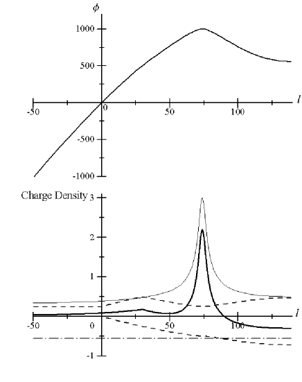
Figure 4: Potential (upper) and charge densities (lower) for Case 1. In the lower figure, the thick solid line is the effective total charge density. Thin solid line, dashed lines, and dash-dotted line are the charge densities due to protons ($-j_{\rm p}/|\beta_{\rm p}|$), injected pairs ($\rho_{-}<0$ and $\rho_{+}>0$), and the constant contribution ($-(j-j_{0})=-0.55$), respectively.

Table 1 indicates that a smaller $\phi_{\rm M}$ and a larger $j_{\rm p}$ lead to a larger amplitude of $E_{\rm F}$, as discussed in Sect. 3.1. In all our examples the PPF ($\phi=0$ and $l=0$) is in region II. The position where the electric field becomes strongest is on the boundary of regions I and II. Since the proton acceleration is slower than the electron acceleration, the boundary is far inside the PPF. For Case 1 the effective charge density becomes zero at $l=-800$ where $\phi=-2\times 10^{4}$. At this point the amplitude of $E$ becomes maximum. In Table 1 we also tabulate the maximum electric field $E_{\rm M}$ numerically obtained. The value of $E_{\rm M}$ rather than $E_{\rm F}$ is the electric field screened in our model. The results show that $E_{\rm M}$ is close to the value in Eq. (25).

Table 1: Model parameters and numerical results for $E_{\rm F}$ and $E_{\rm M}$

	$j_{\rm p}$	$j_{+}$	$\phi_{\rm M}$	$j-j_{0}$	$\alpha_{\phi}$	$|E_{\rm F}|$	$|E_{\rm M}|$
Case 1	0.30	0.25	1000	0.55	$3.2\times 10^{-4}$	18.5	25.7
Case 2	0.30	0.25	600	0.55	$1.6\times 10^{-3}$	21.2	29.3
Case 3	0.90	0.70	1000	1.60	$5.4\times 10^{-4}$	32.9	46.2
Case 4	0.90	0.70	600	1.60	$2.7\times 10^{-3}$	36.8	52.0

Region I ($l\leq-800$) is not shown in Fig. 4. The effective charge density is already positive at the left edge ($l=-50$) of this figure. The density of positrons initially grows outside the PPF, but begins to decrease around the point where the positrons injected at the PPF turn around. Although the total charge density decreases once from this point, the charge density of protons immediately makes the total charge density increase again. In regions III and IV the densities of both pair-electrons and positrons increase while the charge density due to pairs is maintaining, $\bar{\rho}_{+}+\bar{\rho}_{-}\simeq-j_{+}$. The potential of the valley for Case 1 is $\sim 600$ and high enough.

In our examples $\alpha_{\phi}$ turns out to be $10^{-4}$-$10^{-3}$, which is much smaller than the value required in SMT02. In our model the number of electron-positron pairs a beam-electron creates per unit time at the PPF is $E_{\rm F}\alpha_{\phi}\omega_{\rm p}$, which becomes $\sim 2\times 10^{8}T_{0.3}^{1/2}B_{12}^{-1/2}$ ${\rm s^{-1}}$ for Case 1. On the other hand, the photon number a primary beam electron emits per unit time via curvature radiation is $2e^{2}\Gamma/3r\hbar\simeq 10^{7}\Gamma_{6}(r/10^{7}{\rm cm})^{-1}$ ${\rm s^{-1}}$, where $r$ is the radius of curvature of the field line. The resultant number of pairs created from these photons will be of the same order. Although we have adopted a very simple model and estimate the numbers roughly, these numbers are rather close. The required pair creation rate in our examples may be consistent with the conventional pair creation models.

In order to keep the valley shallow enough, our model requires that the negative charge due to pairs flows into region IV, which leads to the negative charge density of $-j_{+}$. Since this charge density is very large compared with $\rho_{\rm in}$, the total effective charge density remains negative in the valley. Therefore, outside the valley the potential grows again. Since the charge density due to protons is a function of only $\phi$, this charge density dominates again as the potential grows, and the potential again begins to decrease at $\phi=\phi_{\rm M}$ again. Electron-positron pairs injected after the peak flow outwards almost at light speed (the lowest $\gamma_{-}$ at the valley is $\sim 100$ for Case 1), so that these pairs do not contribute to the charge density. Reiterating this process, a space charge density wave continues outside the valley. This wave is essentially the same as the wave observed in the numerical solutions in SMT98. Of course, the average effective charge density is zero in this region.

4 CONCLUSIONS AND DISCUSSION

We have shown a possibility that the proton counterflow and injected electron-positron pairs screen a strong electric field expected in the polar cap model. In our numerical examples the required pair creation rate is consistent with the prediction of the conventional pair creation models. A space charge density wave appears outside the PPF in our model. In order to screen a stronger electric field, a larger proton current ($j_{\rm p}\simeq j-j_{+}-j_{0}$) and a smaller potential difference between the PPF and the peak, $\phi_{\rm M}$, are favorable. The values of $\phi_{\rm M}$ and the Lorentz factor of pairs at injection $\bar{\gamma}$ should be the same order.

In addition, the amplitude of the charge density wave should be small enough to keep pair-electrons from returning from outside the screening point. The currents of returning positrons and protons should be comparable, in order to achieve both a small wave amplitude and screening of a large electric field. Since a smaller $\phi_{\rm M}$ requires a higher pair creation rate, the parameter is limited to $\phi_{\rm M}\sim O(10^{3})$. As for the pair Lorentz factor, $\bar{\gamma}\simeq 500$ is the best choice. We found that the non-dimensional electric field our model can screen is a few times ten at most. To attain the Lorentz factor of the primary electron-beam, $\Gamma\sim 10^{6}$, such a value of the electric field requires $\rho_{\rm in}<0.01$, which means that the screening height is greater than $10^{4}$ cm.

In our model the flux of positrons and protons falling onto the star is a few times the GJ flux. The particles falling onto the star heat up the polar caps. The X-ray thermal luminosity from the neutron star investigated by ROSAT (Becker & Trümper, 1997) does not indicate that there is a significant number of particles falling onto the star. Therefore, the fraction of the active region in which the electron beam is accelerated in the whole polar cap region should be small enough in this model.

Our model predicts the appearance of a space charge density wave after the screening. Particles flow forward while accelerating and decelerating in turn. Though the spatial average of the effective charge density is zero, the local charge density is finite. In more realistic cases, the potential wave may not be steady, but oscillate with time. The stability of the potential structure may be determined by the global dynamics in the magnetosphere, which is beyond the scope of this paper. However, the existence of the wave is interesting when we consider the pulsar emission mechanism. The wave may induce the charge bunching that causes coherent radio emission.

If most ions in the co-rotating magnetosphere are Fe irons, the counterflow could be iron flow. In this case the scenario depends on the degree of ionization. If the mass and charge of the Fe irons are $m_{\rm Fe}$ and $qe$, respectively, $\delta$ should be replaced by $\delta^{\prime}=q(m_{\rm p}/m_{\rm Fe})\delta$ in our model. The smaller $q$ becomes, the larger the typical amplitude of the potential variation becomes. Thus we need to adopt a larger value of $\bar{\gamma}$ to avoid electrons returning. Even if Fe irons are fully ionized ($q=26$), $\bar{\gamma}$ is required to be more than $\sim 1000$ in our numerical estimate, while $E_{\rm F}$ becomes larger than in the proton model.