The clustering of Luminous Red Galaxies around Mg ii absorbers

Abstract

We study the cross-correlation between 212 Mg ii quasar absorption systems and $\sim\!\hbox{20,000}$ Luminous Red Galaxies (LRGs) selected from the Sloan Digital Sky Survey Data Release 1 in the redshift range $0.4\!\leq\!z\!\leq\!0.8$. The Mg ii systems were selected to have $\lambda\lambda$2796 & 2803 rest-frame equivalent widths $\geq\!1.0$ Å and identifications confirmed by the Fe ii $\lambda 2600$ or Mg i $\lambda 2852$ lines. Over comoving scales 0.05–13$h^{-1}{\rm\,Mpc}$, the Mg ii–LRG cross-correlation has an amplitude $0.67\pm 0.09$ times that of the LRG–LRG auto-correlation. Since LRGs have halo-masses greater than $3.5\times 10^{12}$ M_⊙ for $M_{R}\!\la\!-21$, this relative amplitude implies that the absorber host-galaxies have halo-masses greater than $\sim 2$–$8\times 10^{11}$ M_⊙. For $10^{13}$ M_⊙ LRGs, the absorber host-galaxies have halo-masses $0.5$–$2.5\times 10^{12}$ M_⊙. Our results appear consistent with those of Steidel et al. (1994) who found that Mg ii absorbers with $W_{\rm r}^{\rm MgII}\!\geq\!0.3$ Å are associated with $\sim\!0.7L_{B}^{*}$ galaxies.

1 Introduction

The connection between quasar (QSO) absorption line systems and galaxies (Bergeron & Boisse, 1991) is important to our understanding of galaxy evolution. Absorption lines provide detailed information about the physical conditions and kinematics of galaxies out to large impact parameters ($R\!\ga\!100{\rm\,kpc}$), regardless of the absorber’s intrinsic luminosity (e.g. Rauch et al., 1996; Ellison et al., 2000). Mg ii $\lambda\lambda$2796 & 2803 are amoungst the most studied metal lines since the doublet signature makes for easy detection.

Past results show that Mg ii absorbers are not unbiased tracers of galaxies but are biased towards late-type galaxies which do not evolve strongly from $z\!\simeq\!1$. The morphological constraints come from imaging by Steidel & Sargent (1992) and Steidel, Dickinson & Persson (1994) who found that Mg ii absorber host-galaxies have $K$-band luminosities consistent with normal $0.7L^{*}_{B}$ Sb galaxies. Further Hubble Space Telescope imaging (Steidel, 1998) indicated that Mg ii absorbers at $z_{\rm abs}\!<\!1$ are drawn from field galaxies of all disk morphological types. These galaxies are also found to have roughly constant star formation rate since $z\!\sim\!1$: from a sample of 58 Mg ii absorbers with rest-frame equivalent widths $W_{\rm r}^{\rm MgII}\!\geq\!0.30$ Å, Steidel et al. (1994) found that the mean rest-frame $M_{B}$ and $B\!-\!K$ colours of the host-galaxies do not evolve in the redshift range $0.2\!<\!z_{\rm abs}\!<\!1$. Furthermore, their rest-frame $K$-band luminosity function (LF) closely matches the $K$-band LF at $z\!=\!0$ down to $0.05L^{*}_{K}$. This ‘no evolution’ picture of the $K$-band LF implies little or no stellar mass evolution from $z\!\simeq\!1$. However, using more direct constraints from deep imaging surveys, Dickinson et al. (2003) and Rudnick et al. (2003) find that the stellar mass increased by a factor of 2 over this epoch. Thus, these earlier studies imply that Mg ii absorption-selected galaxies are biased towards non-evolving, luminous disk morphological types.

From the observed absorber–host-galaxy impact parameter distribution, Steidel (1993, 1995) constrained the cross-section of Mg ii absorbers with $W_{\rm r}^{\rm MgII}\!\geq\!0.30$ Å to have radius $R_{\times}\!\sim\!40h^{-1}{\rm\,kpc}$ (physical, $70h^{-1}{\rm\,kpc}$ comoving). In addition, these systems are always found to be associated with neutral hydrogen absorbers in the Lyman limit regime ($\log\hbox{$N_{\hbox{{\rm H}{\sc\,i}}}$}\!\geq\!3\!\times\!10^{17}{\rm\,cm}^{-2}$).

Little information currently exists about the environment of Mg ii absorbers on scales up to $10h^{-1}{\rm\,Mpc}$. Recently, Haines, Campusano & Clowes (2004) analysed the clustering of early-type galaxies around two Mg ii absorbers at $z_{\rm abs}\!=\!0.8$ & $1.2$ using wide field images ($40\arcmin\times 35\arcmin$). They find a significant excess of galaxies across the field and conclude that large-scale structures containing Mg ii absorbers mark out volumes of enhanced galaxy density.

All the above studies are based on relatively small ($\la\!50$) samples of Mg ii absorbers and, with the exception of Haines et al. (2004), relatively small-area ($\la\!10\arcmin\times 10\arcmin$) galaxy surveys. The Sloan Digital Sky Survey (SDSS; Stoughton et al., 2002) allows us to significantly transcend these limitations. In this paper we use $\sim\!\hbox{20,000}$ Luminous Red Galaxies (LRGs) from SDSS Data Release 1 (DR1; Abazajian et al., 2003; Strauss et al., 2002) to constrain the environment, and more specifically, the mass of the halos associated with 212 Mg ii absorbers. In a hierarchical galaxy formation scenario, the amplitude ratio of the Mg ii–LRG cross-correlation and LRG–LRG auto-correlation is a measure of the relative masses of the halos associated with Mg ii absorbers and LRGs.

Throughout this paper, we adopt $\Omega_{\rm M}\!=\!0.3$, $\Omega_{\Lambda}\!=\!0.7$, $\sigma_{8}=0.8$, and $H_{0}\!=\!100h\,\hbox{${\rm km\,s}^{-1}$}{\rm\,Mpc}^{-1}$. Thus, at $z\!=\!0.6$, $1\arcsec$ corresponds to $7.44h^{-1}{\rm\,kpc}$ and $1\arcmin$ corresponds to $446h^{-1}{\rm\,kpc}$, both comoving. At that redshift $H(z)\!=\!1.39H_{0}$, so $\delta z\!=\!0.1$ corresponds to $216h^{-1}{\rm\,Mpc}$ in comoving coordinates.

2 Sample definitions

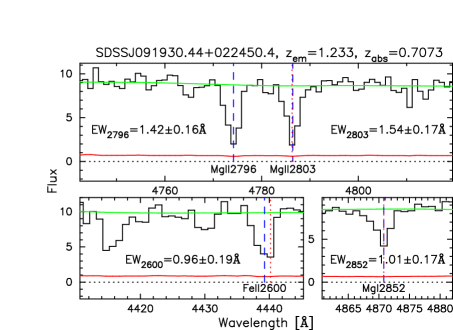
Figure 1: Example Mg ii absorption system showing the Mg ii $\lambda\lambda$2796/2803 doublet and the supporting transitions, Fe ii $\lambda 2600$ and Mg i $\lambda 2852$. Note also the Fe ii $\lambda$2587 line at $\lambda_{\rm obs}\approx 4415$Å. The upper solid line is our fitted continuum and the lower solid line is the $1\,\sigma$ error array.

2.1 Mg ii absorbers

For the 16713 QSO spectra in the SDSS QSO sample of Schneider et al. (2003), we searched for Mg ii $\lambda\lambda$2796/2803 absorption doublets with $\hbox{$z_{\rm abs}$}\leq 0.8$ using a largely automated technique. A third-order polynomial was fitted to overlapping 2500-${\rm km\,s}^{-1}$ sections of each QSO spectrum from 10,000 ${\rm km\,s}^{-1}$ above the Ly$\alpha$ emission line to 10,000 ${\rm km\,s}^{-1}$ below the Mg ii emission line. Pixels with flux $>\!2\,\sigma$ below and $>\!5\,\sigma$ above the continuum are rejected and the continuum is re-fitted to the remaining points. This process is iterated until no more points are rejected. Overlapping portions of adjacent continua are joined by weighting each linearly from zero at the edge to unity at the centre. The final continuum is smoothed over 11 pixels ($\approx\!760$ ${\rm km\,s}^{-1}$). The 2500 ${\rm km\,s}^{-1}$ chunk-size is small enough to fit most emission features but large enough so that strong Mg ii doublets do not cause significant spurious bends in the continuum.

Candidate Mg ii $\lambda 2796$ lines are searched for by identifying the pixel within a $\Delta\lambda_{\rm rest}\!=\!7$ Å sliding window with the most significant flux deviation $>\!2\,\sigma$ below the continuum. This $\Delta\lambda_{\rm rest}$ accounts for most of the Mg ii $\lambda 2796$ absorption while avoiding significant overlap with the Mg ii $\lambda 2803$ line. A similar window is centred on the Mg ii $\lambda 2803$ wavelength with the same redshift, $z_{\rm abs}$, as the putative Mg ii $\lambda 2796$ line. If $W_{\rm r}^{\rm MgII}\!\geq\!1.0$ Å and the mean signal-to-noise ratio (S/N) is $\geq\!10$ within each window, the system is identified as a candidate Mg ii absorber.

Candidates require at least one supporting transition to be considered real detections: Fe ii $\lambda 2600$ or Mg i $\lambda 2852$. Fe ii is the preferred line since it is stronger than Mg i. Fe ii $\lambda 2600$ is, in principle, detectable in SDSS spectra when $\hbox{$z_{\rm abs}$}\!\ga\!0.47$ (i.e. $\lambda_{\rm obs}\!\ga\!3800$Å) and so we use the criterion advocated by Nestor et al. (2003) to select for damped Ly$\alpha$ systems (DLAs), $W_{\rm r}^{\rm FeII}\!\geq\!0.5$Å. If Fe ii $\lambda 2600$ is not detectable or if ${\rm S/N}\!<\!10$ in the Fe ii $\lambda 2600$ window, we require that Mg i $\lambda 2852$ is detected with ${\rm S/N}\!\geq\!10$ and ${W_{\rm r}^{\rm MgI}\!\geq\!0.2}$Å. Several caveats apply to the above requirements, particularly when one or more transitions fall near emission features and the broad absorption features often associated with them. We will describe these caveats in detail in a later paper, suffice it to note here that they apply to $\la\!20$ per cent of (real) systems.

Finally, we remove clearly spurious candidates by visually inspecting each Mg ii spectrum. The most common mis-identification is broad C iv absorption near the C iv emission line.

With the above algorithm we detected and visually confirmed 212 Mg ii absorbers in the DR1. A typical Mg ii absorption doublet is shown in Fig. 1. Note that, in addition to the crucial lines for selection, the Fe ii $\lambda$2587 line also often confirms the detection. We provide a catalogue of the Mg ii absorbers in Table 1 and the absorption redshift distribution is shown in Fig. 2.

Table 1: Catalogue of 212 Mg ii absorbers from the SDSS DR1 with $0.4\!\leq\!z_{\rm abs}\!\leq\!0.8$. The J2000 name, QSO and absorption redshifts and the measured $W_{\rm r}$ for Mg ii$\lambda\lambda$2796 & 2803, Mg i $\lambda 2852$ and Fe ii $\lambda 2600$ are given. Here we show only a small sample from the full table which is available in the electronic edition of this paper and from http://www.ast.cam.ac.uk/$\sim$mim/pub.html. Full name designations and statistical uncertainties in $W_{\rm r}$ are given in the electronic version.

			Rest equivalent width $\left[{\rm\AA}\right]$
SDSSJ	$z_{\rm qso}$	$z_{\rm abs}$	2796	2803	2852	2600
004041$-$005537	2.090	0.6612	4.37	3.46	0.86	1.83
004721$+$154652	1.272	0.7742	1.31	1.92	0.57	1.12
005130$+$004150	1.190	0.7394	2.19	1.71	0.58	1.27
005408$-$094638	2.128	0.4778	2.18	2.09	1.20	2.17

2.2 Luminous red galaxies

SDSS DR1 contains more than $10^{6}$ LRGs over $\sim\!2000$ sq. degrees which have luminosities $M_{g}\!<\!-21$ and fall on the red sequence with $(u\!-\!g)_{0}\!\simeq\!2$ (Eisenstein et al., 2001; Scranton et al., 2003).

For each Mg ii absorber, galaxies meeting the following criteria were extracted from the SDSS DR1 galaxy catalogue:

$$i^{*}_{\rm petro} < 21,$$ (1)

$$0.7(g^{*}-r^{*})+1.2[(r^{*}-i^{*})-0.18] > 1.6\,,$$ (2)

$$(g^{*}-r^{*}) > 1\,,$$ (3)

$$({\rm d}_{\perp}\equiv)(r^{*}-i^{*})-(g^{*}-r^{*})/8 > 0.4\,,$$ (4)

$$r^{*}_{\rm psf}-r^{*}_{\rm model} > 0.3\,,$$ (5)

$$\left|z_{\rm phot}-z_{\rm abs}\right| < 0.05\,.$$ (6)

We also required errors on the model magnitudes to be less than $0.2{\rm\,mag}$ in $r^{*}$ and $i^{*}$, and we excluded objects flagged by SDSS as BRIGHT, SATURATED, MAYBE_CR or EDGE. The model magnitudes were used to compute the colours. Equations (1)–(4) are the LRG selection criteria of Scranton et al. (2003). Criterion 4 is equivalent to imposing $z_{\rm phot}\!\ga\!0.3$. Criterion 5 separates stars from galaxies. Criterion 6 is the selection of galaxies within a redshift slice of width $W_{z}\!=\!0.1$ around $z_{\rm abs}$ using the photometric redshifts, $z_{\rm phot}$, of Csabai et al. (2003) who showed these to be accurate to $\sigma_{z}\!=\!0.1$ at $r^{\prime}\!<\!21$. The choice of the slice width $W_{z}\!=\!0.1$ corresponds to $\sim\!200h^{-1}{\rm\,Mpc}$ (co-moving) and is arbitrary. It is a compromise to optimise the signal-to-noise: too small a width will yield too few correlated pairs, too large a width will wash out the signal. Finally, we remove the 10 per cent of the galaxies with problematic photometric redshifts by requiring that galaxies have $z_{\rm phot}$ uncertainties $\sigma_{z_{\rm phot}}\!<\!0.5$. A total of 33,348 galaxies met all these criteria in our 212 fields ($\sim\!300$ sq. degrees). Fig. 2 shows the redshift distribution of these LRGs for the 212 fields. We used the spectroscopic redshift when available, which includes only $\sim\!160$ LRGs. This situation will change in the future with the 2dF/SDSS program to obtain spectra of LRGs.

Figure 2: Redshift distribution of the LRGs (bottom) and Mg ii systems (top). The solid curve shows the LRG distribution smoothed with a Gaussian kernel. The inset shows the distribution of QSO emission redshifts.

LRGs are expected to have halo-masses $>\!10^{12}$ M_⊙. Brown et al. (2003) showed that the clustering of red ($B_{W}\!-\!R\!>\!1.44$) galaxies between $z\!=\!0.3$ and $0.9$ in the NOAO deep wide survey is a strong function of luminosity: in the luminosity range $-21.5\!<\!M_{R}\!<\!-20.5$, the correlation length is $6.3\pm 0.5h^{-1}{\rm\,Mpc}$, and rapidly increases to $11.2h^{-1}{\rm\,Mpc}$ at $M_{R}\!=\!-22$. Such strong clustering is consistent with halo-masses of $3.5\times 10^{12}$ to $3\times 10^{13}$ M_⊙ using the bias prescription of Mo & White (2002).

3 Results

3.1 Theoretical background

A widely used statistic to measure the clustering of galaxies is the correlation function, $\xi(r)$. The absorber–galaxy cross-correlation, $\xi_{\rm ag}$, is defined from the conditional probability of finding a galaxy in a volume d$V$ at a distance $r=|\mathbf{r}_{2}\!-\!\mathbf{r}_{1}|$, given that there is a Mg ii absorber at $\mathbf{r}_{1}$:

$$P({\rm LRG}|\hbox{{\rm Mg}{\sc\,ii}})=\overline{n}_{u}\left[1+\xi_{\rm ag}(r)\right]\mathrm{d}V,$$ (7)

where $\overline{n}_{u}$ is the unconditional background galaxy density.

The observed amplitudes of the auto- and cross-correlation functions are related to the dark matter correlation function, $\xi_{\rm DM}$, through the bias, $b(M)$, which is a function of the dark matter halo-mass (e.g. Mo et al., 1993; Mo & White, 2002):

$$\xi_{\rm gg}(r) = b^{2}(M_{\rm g})\,\xi_{\rm DM}(r)\,,$$ (8)

$$\xi_{\rm ag}(r) = b(M_{\rm a})\,b(M_{\rm g})\,\xi_{\rm DM}(r)\,.$$ (9)

Thus, the amplitude ratio of the cross- to auto-correlation, which is $(r_{\rm 0,ag}/r_{\rm 0,gg})^{\gamma}$ for $\xi(r)=(r/r_{0})^{-\gamma}$, is a measurement of the bias ratio $b(M_{\rm a})/b(M_{\rm g})$ which in turn yields the relative halo-masses ($M_{\rm a}/M_{\rm g}$). This assumes that $\xi_{\rm ag}$ and $\xi_{\rm gg}$ have the same slope $\gamma$.

Since our LRG sample is made up of galaxies with photometric redshifts, we computed the projected cross- and auto-correlation functions, i.e. as a function of physical distance $r_{\theta}=D_{A}(1+z)\theta$ in comoving Mpc with $D_{A}$ the angular diameter distance. From the definitions of $w_{\rm gg}(r_{\theta})$ (e.g. Phillipps et al., 1978; Peebles, 1993) and $w_{\rm ag}(r_{\theta})$ (e.g. Eisenstein, 2003; Adelberger et al., 2003), the amplitude of both $w_{\rm gg}(r_{\theta})$ and $w_{\rm ag}(r_{\theta})$ is inversely proportional to $1/W_{z}$, where $W_{z}$ is the width of redshift distribution $\frac{\mathrm{d}N}{\mathrm{d}z}$. For a top-hat $\frac{\mathrm{d}N}{\mathrm{d}z}$, the ratio $w_{\rm ag}(r_{\theta})/w_{\rm ag}(r_{\theta})$ is exactly the bias ratio $b(M_{\rm a})/b(M_{\rm g})$, irrespective of $W_{z}$ . In the case of a Gaussian redshift distribution $\frac{\mathrm{d}N}{\mathrm{d}z}$, $w_{\rm ag}(r_{\theta})/w_{\rm ag}(r_{\theta})$ is overestimated by $25\pm 10$ per cent. This factor was determined using (i) numerical integration and (ii) mock catalogues (from the GIF2 collaboration, Gao et al., 2004) made of galaxies that had a redshift uncertainty equal to the slice width, $W_{z}$, as in the case of our LRG sample. Note that this factor depends on the shape of $\frac{\mathrm{d}N}{\mathrm{d}l}$, not its width.

3.2 Mg ii–luminous red galaxy cross-correlation

Fig. 3 (filled circles) shows $w_{\rm ag}$ for the entire sample, where we used the following estimator of $w_{\rm ag}(r_{\theta})$ (also advocated by Adelberger et al., 2003):

$$1+w_{\rm ag}(r_{\theta})=\frac{\rm AG}{\rm AR}\,,$$ (10)

where AG is the observed number of absorber–galaxy pairs between $r_{\theta}-dr/2$ and $r_{\theta}+\mathrm{d}r/2$, summed over all the fields. AR is the normalized absorber–random galaxy pairs where the normalization is applied to each field independently: ${\rm AR}\!=\!\sum_{i}{\rm AR}^{i}\;N_{g}^{i}/N_{r}^{i}$, where ARⁱ is the number of random pairs in field $i$, and $N_{g}^{i}$ ($N_{r}^{i}$) is the total number of galaxies (random galaxies) for that field. From the sample of 33,348 objects within the initial search radius of $40\arcmin$, there are 19,496 objects within $r_{\theta}\!=\!12.8h^{-1}{\rm\,Mpc}$ which is the outer radius of the largest bin used. Taking into account the areas missing from the SDSS within our search radius, we generated approximately $200$ times more random galaxies to reduce the shot noise of AR to an insignificant proportion. Table 2 shows the total number of pairs, AG, and the expected number of pairs, AR, if Mg ii absorbers and LRGs were not correlated.

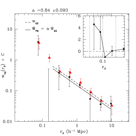
Figure 3: The projected Mg ii–LRG cross-correlation, $w_{\rm ag}(r_{\theta})$, for 212 Mg ii absorbers and 19,496 LRGs is shown by the filled circles. The error bars are computed using the Jackknife technique. The filled triangles show the LRG–LRG auto-correlation, $w_{\rm gg}$, offset by 0.025 in $r_{\theta}$ for clarity, and the dashed line shows the fit to $w_{\rm gg}$. The solid line shows the relative amplitude of $w_{\rm ag}$ and $w_{\rm gg}$, i.e. using $\hat{w}_{\rm ag}=a\times\hat{w}_{\rm gg}$ for scales $r_{\theta}\!>\!200h^{-1}{\rm\,kpc}$ since the smallest scales will be affected by the finite cross-section of the absorbers. The best-fitting relative amplitude is $a\!=\!\hbox{$0.84\pm 0.09$}$. The inset shows the first two bins, 50–100$h^{-1}{\rm\,kpc}$ and $100$–$200h^{-1}{\rm\,kpc}$ (dotted lines), split into two sub-bins. The third sub-bin, 100–150$h^{-1}{\rm\,kpc}$, contains no galaxies due to the absorber cross-section effects.

The $w_{\rm ag}$ error bars are computed using the jackknife estimator (Efron, 1982): we divide the sample into 10 parts and compute the covariance matrix from the $N_{\rm jack}\!=\!10$ realisations for each part:

$${\rm COV}_{ij}=\frac{N_{\rm jack}-1}{N_{\rm jack}}\sum_{k=1}^{N_{\rm jack}}[w_{k}(r_{\theta_{i}})-\overline{w}(r_{\theta_{i}})]\cdot[w_{k}(r_{\theta_{j}})-\overline{w}(r_{\theta_{j}})]$$ (11)

where $w_{k}$ is the $k$th measurement of the cross-correlation and $\overline{w}$ is the average of the $N_{\rm jack}$ measurements.

Table 2: The total number of absorber–LRG pairs AG and the number of absorber–random pairs AR, for the cross-correlation shown in Fig. 3. The number of pairs expected if one extrapolated $w_{\rm ag}$ to $r_{\theta}\!<\!0.2h^{-1}{\rm kpc}$ are shown in parentheses (see text).

$r_{\theta}$	AG	AR	$w_{\rm ag}$	$\sigma(w)$
[$h^{-1}{\rm\,Mpc}$]
0.05–0.1	4(2.5)	0.834	3.797	2.40
0.1–0.2	3(7)	3.45	$-$0.135	0.625
0.2–0.4	20	14.7	0.361	0.274
0.4–0.8	72	57.1	0.261	0.146
0.8–1.6	263	232	0.134	0.0265
1.6–3.2	956	925	0.0330	0.0457
3.2–6.4	3702	3650	0.0154	0.0132
6.4–12.8	14439	14200	0.0171	0.0281

Two important internal consistency checks on these results were performed: using either synthetic Mg ii absorbers with real LRGs or synthetic LRGs with real Mg ii absorbers, we find no cross-correlation signal.

3.3 Relative amplitude of cross- and auto-correlation

In order to constrain the amplitude of $w_{\rm ag}$ with respect to that of the LRG–LRG auto-correlation $w_{\rm gg}$, we use the following estimator with the same galaxies used for the cross-correlation:

$$1+w_{\rm gg}(r_{\theta})=\frac{\rm GG}{\rm GR}\,.$$ (12)

GG is the total observed number of galaxy–galaxy pairs between $r_{\theta}-\mathrm{d}r/2$ and $r_{\theta}+\mathrm{d}r/2$ and GR is the total galaxy–random galaxy pairs, computed as before. The filled triangles in Fig. 3 show $w_{\rm gg}$. The errors and the covariance matrix for $w_{\rm gg}$ are computed using $N_{\rm jack}\!=\!10$ jackknife realisations.

The arguments in section 3.1 require that both $w_{\rm ag}$ and $w_{\rm gg}$ have the same slope $\gamma$. Therefore, to constrain the amplitude ratio $w_{\rm ag}/w_{\rm gg}$, we first fitted a power law to $w_{\rm gg}(r_{\theta})$, and used that as a model for ${w}_{\rm gg}$. We will only use the scales larger than $200h^{-1}{\rm\,kpc}$ in the rest of this paper in order to avoid possible cross-section effects (discussed at the end of this section).

First, the model $\hat{w}_{\rm gg}(r_{\theta})=A_{\rm gg}r_{\theta}^{\beta_{\rm gg}}$ for $w_{\rm gg}$ gives a best amplitude, $A_{\rm gg}$, at $1h^{-1}{\rm\,Mpc}$ and slope $\beta_{\rm gg}$ of $0.175\pm 0.028$ and $-0.780\pm 0.147$ respectively . The fitted power law $\hat{w}_{\rm gg}(r_{\theta})$ is shown by the dashed line in Fig. 3.

Then, from the following model for $w_{\rm ag}$,

$$\hat{w}_{\rm ag}=a\times\hat{w}_{\rm gg},$$ (13)

where $a$ is the amplitude ratio $A_{\rm ag}/A_{\rm gg}$, we find that the best amplitude ratio

$$a=\hbox{$0.84\pm 0.09$}$$ (14)

by minimizing $\chi^{2}\propto[\mathbf{w}-\mathbf{\hat{w}}]^{T}\mathrm{COV}^{-1}[\mathbf{w}-\mathbf{\hat{w}}]\,,$ where $\mathbf{w}$ and $\mathbf{\hat{w}}$ are the vector data and model respectively and ${\rm COV}^{-1}$ is the inverse of the covariance matrix, calculated using single value decomposition techniques (see discussion in Bernstein, 1994). This value is consistent with the fact that 5 of the 6 bins of $w_{\rm ag}$ at $r_{\theta}>200h^{-1}$ kpc are below $w_{\rm gg}$ (Fig. 3). Furthermore, the average of the bin ratios $w_{\rm ag}(r_{\theta})/w_{\rm gg}(r_{\theta})$ gives 0.85, close to $0.84\pm 0.09$. Fig. 3 shows both $\hat{w}_{\rm ag}$ (solid line) and $\hat{w}_{\rm gg}$ (dashed line).

For completeness, a power law fit to $w_{\rm ag}(r_{\theta})$, i.e. $\hat{w}_{\rm ag}(r_{\theta})=A_{\rm ag}r_{\theta}^{\beta_{\rm ag}}$, gives $A_{\rm ag}=\hbox{$0.179\pm 0.026$}$, the fitted amplitude at $1h^{-1}{\rm\,Mpc}$, , and $\beta_{\rm ag}\hbox{$-0.955\pm 0.118$}$, the slope.

Note that the relative amplitude, $a$, is free of systematics from contaminants (e.g. stars). This is due to the fact that (1) we use the same galaxies for $w_{\rm ag}$ and $w_{\rm gg}$, and (2) the estimators in equations 10 and 12 are both $\propto 1/N_{g}$, where $N_{g}$ is the number of galaxies. Any contaminants will affect the cross- and auto-correlation function in exactly the same way. We find that $a$ is also robust under numerous different cuts and subsamples. For example, a more restrictive star–galaxy separation [equation (5)] gives consistent results. Similarly, $a$ is robust to a more stringent cut on the redshift difference between the LRGs and Mg ii absorbers than in equation (6). Finally, there is no significant variation in $a$ when excluding LRGs with larger or smaller SDSS magnitude errors.

If the Mg ii cross-section radius ($R_{\times}$) is larger than some of the radial bins, this will affect $w_{\rm ag}(r_{\theta})$ and there will be a redistribution of galaxies in the bins near $r_{\theta}\!\simeq\!R_{\times}$. Steidel (1995) constrained $R_{\times}$ to be $\sim 70h^{-1}{\rm\,kpc}$ (comoving) for absorbers with $W_{\rm r}^{\rm MgII}\!\geq\!0.3$ Å. In fact, we find that (1) the first bin at $r_{\theta}\!=\!50$–$100h^{-1}{\rm\,kpc}$ is higher than expected if $w_{\rm ag}$ is a single power law extrapolated from the large scales (see Table 2); (2) the second bin at $r_{\theta}\!=\!100$–$200h^{-1}{\rm\,kpc}$ is negative and 2$\,\sigma$ below the fit in Fig. 3. The inset in Fig. 3 focuses on these two bins (indicated by the vertical dotted lines) which are divided into two smaller sub-bins. The region from $r_{\theta}\!\sim\!100h^{-1}$ to $150h^{-1}{\rm\,kpc}$ (comoving) contains no galaxies. Note that since we used projected correlations $w(r_{\theta})$, this region corresponds to different angular scales for the range of absorber redshifts, $0.4\!<\!z_{\rm abs}\!<\!0.8$. We also find that this signature is present even with less restrictive samples. We speculate that given the results of Steidel (1995), this deficit of galaxies at $r_{\theta}\!=\!100$–$150h^{-1}{\rm\,kpc}$ is a signature of $R_{\times}$. However, it could be due to some other physical process that prevent pairs at that particular scale. In a future paper, we will explore these hypotheses with larger data sets and simulations.

4 Summary and Discussion

From the SDSS DR1, we selected $\sim\!\hbox{20,000}$ LRGs and 212 Mg ii absorbers with $W_{\rm r}^{\rm MgII}\!\geq\!1$ Å for Mg ii $\lambda\lambda$2796 & 2803 and $W_{\rm r}^{\rm FeII}\!\geq\!0.5$Å for Fe ii $\lambda 2600$. We have examined the clustering of these LRGs around the Mg ii absorbers with unprecedented statistics on small and large scales ($0.05\!\la\!r_{\theta}\!\la\!13h^{-1}{\rm Mpc}$). The amplitude of the Mg ii-LRG cross-correlation relative to that of the LRG–LRG auto-correlation is $0.67\pm 0.07\pm{0.05}$, after applying a correction of $25\pm 10$ per cent discussed in section 3.1 and in the Appendix. The two error terms reflect the statistical and systematic uncertainty, respectively. By adding the errors in quadrature,

$$a=\hbox{$0.67\pm 0.09$}\,.$$ (15)

This corresponds to a correlation length $r_{\rm 0,ag}=(a)^{1/1.8}r_{\rm 0,gg}=5.04^{+0.62}_{-0.63}h^{-1}$ Mpc for $w_{\rm ag}$, and $r_{\rm 0,aa}=(a)^{2/1.8}r_{\rm 0,gg}=4.04^{+0.78}_{-0.78}h^{-1}$ Mpc for the Mg ii–Mg ii autocorrelation $w_{\rm aa}$, where we used the minimum auto-correlation length $r_{\rm 0,gg}=6.3\pm 0.5h^{-1}{\rm\,Mpc}$ of LRGs from Brown et al. (2003).

Within the context of hierarchical galaxy formation [equations (8–9)], equation 15 implies that our Mg ii absorbers have halo masses 4–20 times smaller than the LRG mininum-mass ($3.5\times 10^{12}$ M_⊙), or $\sim 2$–$8\times 10^{11}$ M_⊙. For $10^{13}$ M_⊙ LRG halos, the Mg ii absorbers have halos of $0.5$–$2.5\times 10^{12}$ M_⊙.

Is our mass constraint of Mg ii absorbers in agreement with the results of Steidel et al. (1994) who found that Mg ii absorbers with $W_{\rm r}^{\rm MgII}\!\geq\!0.3$ Å are associated with $\sim\!0.7L_{B}^{*}$ galaxies? Our mass measurement appears broadly consistent with those results given that $\sim L_{B}^{*}$ galaxies have halos of mass $\sim\!10^{12}$M_⊙. Furthermore, the expected amplitude ratio is $\sim\!0.70$, close to our $a\!=\!0.67$. The expected amplitude ratio is found assuming that the correlation length does not evolve from $z=0.5$ to $z=0$ and using the local correlation of early and late type galaxies. At $z=0$, Shepherd et al. (2001) found that the early- and late-type galaxy auto-correlation lengths were $r_{0}\!=5.45{\rm\,Mpc}$ and $3.95$ respectively. Budavári  et al. (2003) found $r_{0}\!=6.5{\rm\,Mpc}$ and $4.5$ respectively. Assuming $\gamma\!=\!1.8$ for both of these auto-correlations, then from equations 8 & 9 one expects the late–early cross-correlation amplitude to be $(3.95/5.45)^{1.8/2}\!\simeq\!0.74$ (0.72 for Budavári  et al., 2003) times that of the auto-correlation.

Note that there are important differences between our Mg ii sample and that of Steidel et al. (1994). Firstly, our larger equivalent width threshold, $W_{\rm r}^{\rm MgII}\!\geq\!1$ Å, will preferentially select systems with a larger velocity dispersion over the absorption components. Thus, our sample is potentially biased towards more massive halos. Secondly, our Mg ii sample will be dominated by DLAs: Rao & Turnshek (2000) find that $\sim\!50$ per cent of systems with $W_{\rm r}^{\rm MgII}\!\geq\!0.5$ Å and $W_{\rm r}^{\rm FeII}\!\geq\!0.5$ Å are DLAs. Nestor et al. (2003) use $W_{\rm r}^{\rm MgII}\!\geq\!1$ Å to select a larger proportion of DLAs.

It should be emphasized that this method (i.e. measuring a correlation ratio) has the following advantages: (i) it is free of systematics from contaminants (e.g. stars), (ii) it does not require knowledge of the true width of the redshift distribution, and (iii) it constrains the masses of the Mg ii/DLA host-galaxies in a statistical manner without directly identifying them. Thus, with a sample of confirmed DLAs which are not selected on the basis of Mg ii line-strength, one should be able to derive the mean mass of the DLA host-galaxies with only relatively shallow wide-field imaging. This could help establish the relative proportions of low- and high-luminosity contributions to DLA host-galaxies. This topic is currently under some debate (e.g. compare Rao et al. 2003 and Chen & Lanzetta 2003).

Appendix A On correlation functions

It may seem that taking the ratio between the cross- and auto-correlation is inappropriate since the former is based on absorbers with spectroscopic (i.e. accurate) redshifts and a sample of galaxies with photometric redshifts (accurate only to $\sigma_{z}\simeq 0.1$), while the latter comprises only galaxies with photometric redshifts. In this paper, we have measured the projected correlation function $w_{\rm p}(r_{\theta})$. For a given field (with one absorber) with galaxies distributed with $\frac{\mathrm{d}N}{\mathrm{d}z}$, one may think that the auto-correlation is proportional to $\int\left(\hbox{$\frac{\mathrm{d}N}{\mathrm{d}z}$}\right)^{2}\mathrm{d}z$ while the cross-correlation is proportional to $\int\left(\hbox{$\frac{\mathrm{d}N}{\mathrm{d}z}$}\right)^{1}\mathrm{d}z$. Thus, at first glance, their ratio is therefore not very useful. Below we show the situation to be not so trivial.

First, some definitions and results that will be useful later. For a 3D correlation function $\xi(r)=(r/r_{0})^{-\gamma}$, the projected correlation function $w_{\rm p}(r_{\rm p})$ is (Davis & Peebles, 1983):

$$w_{\rm p}(r_{\rm p}) = \int_{\infty}^{\infty}\mathrm{d}y\;\xi(r_{\rm p},y)=\int_{\infty}^{\infty}\mathrm{d}y\;\xi(\sqrt{r_{\rm p}^{2}+y^{2}})$$ (16)

$$= (r_{\rm p})^{1-\gamma}\;r_{0}^{\gamma}\;H_{\gamma}$$

where $\xi(r_{\rm p},y)$ is the 3D correlation function decomposed along the line of sight $y$ and on the plane of the sky $r_{\rm p}$, i.e. $r^{2}=y^{2}+r_{\rm p}^{2}$. $H_{\gamma}$ is in fact the Beta function $B(a,b)=\int_{0}^{1}t^{a-1}\;(1-t)^{b-1}\;\mathrm{d}t$ evaluated with $a=1/2$ and $b=(\gamma-1)/2$, i.e. $H_{\gamma}=B(\frac{1}{2},\frac{\gamma-1}{2})=\hbox{$\Gamma(\frac{1}{2})\Gamma(\frac{\gamma-1}{2})/\Gamma(\frac{\gamma}{2})$}$.

In appendix C of Adelberger et al. (2003), one finds the expected number of neighbours between $r_{\theta}-\mathrm{d}r/2$ and $r_{\theta}+\mathrm{d}r/2$ within a redshift distance $|\Delta_{z}|\!<\!r_{\rm z}$:

$$w_{\rm p}(r_{\theta}\!<\!r_{\rm z}) = \frac{1}{r_{\rm z}}\int_{0}^{r_{z}}\mathrm{d}l\;\xi(\sqrt{r_{\theta}^{2}+l^{2}})$$ (17)

$$= \frac{1}{2r_{z}}(r_{\theta})^{1-\gamma}\;r_{0}^{\gamma}\;H_{\gamma}\;I_{x}(\frac{1}{2},\frac{\gamma-1}{2})$$

where $x=r_{\rm z}^{2}/(r_{\rm z}^{2}+r_{\theta}^{2})$ and $I_{x}$ is the incomplete Beta function $B_{x}(a,b)=\int_{0}^{x}t^{a-1}\;(1-t)^{b-1}\;\mathrm{d}t$ normalized by ${B(a,b)}$: $I_{x}(a,b)\equiv B_{x}(a,b)/B(a,b)$.

Many papers (Phillipps et al., 1978; Peebles, 1993; Budavári  et al., 2003) have shown that the angular correlation function is

$$w(\theta)=(\theta)^{1-\gamma}\;r_{0}^{\gamma}\;H_{\gamma}\times\int_{0}^{\infty}\mathrm{d}z\left(\hbox{$\frac{\mathrm{d}N}{\mathrm{d}z}$}\right)^{2}g(z)^{-1}f(z)^{1-\gamma}$$ (18)

where $g(z)=\mathrm{d}r/\mathrm{d}z=c/H(z)$ and $f(z)=D_{c}(z)$ is the comoving line-of-sight distance to redshift $z$, i.e. $D_{c}(z)=\int_{0}^{z}\mathrm{d}t\frac{c}{H(t)}$.

Equation 18 can be derived from the definitions of the angular and 3D correlation functions, $w(\theta)$ and $\xi(r)$ (e.g. Phillipps et al., 1978). We reproduce the derivation here and extend it to projected auto- and cross-correlation functions. The probabilities of finding a galaxy in a volume d$V_{1}$ and another in a volume d$V_{2}$ at a distance $r=|\mathbf{r}_{2}\!-\!\mathbf{r}_{1}|$, along two lines of sight separated by $\theta$ are

$$\mathrm{d}P(\theta) = {\cal N}^{2}\;\mathrm{d}\Omega_{1}\mathrm{d}\Omega_{2}[1+w(\theta)]\,\hbox{or}$$ (19)

$$\mathrm{d}P(r) = n(z)^{2}\;\mathrm{d}V_{1}\mathrm{d}V_{2}[1+\xi(r)]$$ (20)

where $\cal N$ is the number of galaxies per solid angle, i.e. $\mathrm{d}N/\mathrm{d}\Omega$, and $n(z)$ is the number density of galaxies, which can be a function of redshift. Given that ${\cal N}=\frac{1}{\mathrm{d}\Omega}\int\,n(z)\mathrm{d}V(z)$ and that $\mathrm{d}V=f^{2}(z)g(z)\mathrm{\;}d\Omega\mathrm{d}z$, ${\cal N}\equiv\int\mathrm{d}z\;\hbox{$\frac{\mathrm{d}N}{\mathrm{d}z}$}=\int\mathrm{d}z\;n(z)f^{2}(z)g(z)$.

To relate $w(\theta)$ and $\xi(r)$, one needs to integrate equation 20 over all possible lines-of-sight separated by $\theta$ (i.e. along $z_{1}$ and $z_{2}$) and equate it with equation 19:

$${\cal N}^{2}[1+w(\theta)] = \int_{0}^{\infty}\mathrm{d}z_{1}f(z_{1})^{2}g(z_{1})n(z_{1})\cdot$$ (21)

$$\int_{0}^{\infty}dz_{2}f(z_{2})^{2}g(z_{2})n(z_{2})[1+\xi(r_{12})]\;.$$

In the regime of small angles, the distance $r_{12}$ (in comoving Mpc) can be approximated by:

$$r_{12}^{2} = r_{1}^{2}+r_{2}^{2}-2r_{1}r_{2}\cos\theta$$ (22)

$$\simeq (r_{1}-r_{2})^{2}+r^{2}\theta^{2}\quad\hbox{with}\;r=\frac{r_{1}+r_{2}}{2}$$

$$\simeq (g(z)(z_{1}-z_{2}))^{2}+f(z)^{2}\theta^{2}\quad\hbox{with}\;z=\frac{z_{1}+z_{2}}{2}$$

$$\simeq g(z)^{2}y^{2}+f(z)^{2}\theta^{2}\quad\hbox{with}\;y={z_{1}-z_{2}}\,.$$

Changing variables in equation 21 from ($z_{1},z_{2}$) to ($z,y$), assuming the the major contribution is from $z_{1}\simeq z_{2}$ and using equation 22, the angular correlation function is

$$w(\theta)=\frac{\int_{0}^{\infty}dzf(z)^{4}g(z)^{2}n(z)^{2}\int_{-\infty}^{\infty}\mathrm{d}y\xi(\sqrt{f(z)^{2}\theta^{2}+g(z)^{2}y^{2}})}{\left[\int_{0}^{\infty}dzf^{2}(z)g(z)n(z)\right]^{2}}\,.$$ (23)

Changing variables to $l=g(z)y$, using equation 16 and using a normalized redshift distribution, i.e. $\int\mathrm{d}z\;\hbox{$\frac{\mathrm{d}N}{\mathrm{d}z}$}=1$, equation 23 becomes

$$w(\theta)=\int_{0}^{\infty}dz\left(\hbox{$\frac{\mathrm{d}N}{\mathrm{d}z}$}\right)^{2}g(z)^{-1}\times(f(z)\theta)^{1-\gamma}\;r_{0}^{\gamma}\;H_{\gamma}$$ (24)

which leads to equation 18 (equation 9 in Budavári  et al., 2003) and is one version of Limber’s equations.

In this paper, we measured the projected auto-correlation of the LRGs, $w_{\rm gg}(r_{\theta})$, where $r_{\theta}=f(z)\theta$ . Following the same steps as above with $r_{\theta}$ instead of $\theta$, and $\mathrm{d}V=(\mathrm{d}r_{\theta})^{2}g(z)\mathrm{d}z$, $w_{\rm gg}(r_{\theta})$ is:

$$w_{\rm gg}(r_{\theta})=r_{\theta}^{1-\gamma}\;r_{\rm 0,gg}^{\gamma}\;H_{\gamma}\int_{0}^{\infty}dz\left(\hbox{$\frac{\mathrm{d}N}{\mathrm{d}z}$}\right)^{2}g(z)^{-1}$$ (25)

In the case of the projected cross-correlation, $w_{\rm ag}(r_{\theta})$, the conditional probability of finding a galaxy in the volume $\mathrm{d}V_{2}$ given that there is an absorber at a known position $\mathbf{r}_{1}$ is, by definition (e.g. Eisenstein, 2003),

$$\mathrm{d}P(2|1)(\theta) = {\cal N}_{\rm g}\;\mathrm{d}\Omega_{2}[1+w_{\rm p}(r_{\theta})]$$ (26)

$$\mathrm{d}P(2|1)(r) = n_{\rm g}(z)\;\mathrm{d}V_{2}[1+\xi(r)]\,.$$ (27)

Using the same approximations (equation 22) and one integral along the line of sight $z_{2}$ (keeping the absorber at $z_{1}$), one finds that the projected cross-correlation is:

$$w_{\rm ag}(r_{\theta}) = \int_{0}^{\infty}dz_{2}f(z_{2})^{2}g(z_{2})n(z_{2})\xi(r_{12})$$ (28)

$$= \int_{0}^{\infty}dz\left(\hbox{$\frac{\mathrm{d}N}{\mathrm{d}z}$}\right)\xi(\sqrt{r_{\theta}^{2}+g(z)^{2}(z_{1}-z_{2})^{2}})$$

$$= \int_{0}^{\infty}dy\,g(z)\left(\hbox{$\frac{\mathrm{d}N}{\mathrm{d}z}$}\right)g(z)^{-1}\xi(\sqrt{r_{\theta}^{2}+g(z)^{2}y^{2}})$$

$$= \int_{0}^{\infty}dl\frac{\mathrm{d}N}{\mathrm{d}l}\xi(\sqrt{r_{\theta}^{2}+l^{2}})$$

$$\simeq \frac{1}{W_{z}}\times(r_{\theta})^{1-\gamma}\;r_{\rm 0,ag}^{\gamma}\;H_{\gamma}\,,$$ (29)

where we approximated $\frac{\mathrm{d}N}{\mathrm{d}z}$ with a normalized top-hat of width $W_{z}=2r_{z}$, used equation 17, and the fact that $I_{x}\simeq 1$ since $x\simeq 1$ for a typical width $W_{z}$ of 200$h^{-1}$ Mpc (Section 2.2). Thus, as one would have expected, the cross-correlation is inversely proportional to the width of the galaxy distribution. Naturally, in equation 26 and 27, the redshift of galaxy 1 (i.e. the absorber) is assumed to be known with good precision. If the absorber population had poorly known redshifts, one would need to add an integral to equation 28, washing out the cross-correlation signal further. This is not an issue for our Mg ii absorbers.

For the projected auto-correlation (equation 25), if one approximates $\frac{\mathrm{d}N}{\mathrm{d}z}$ by a top-hat function of width $W_{z}$, then

$$w_{\rm gg}(r_{\theta}) = (r_{\theta})^{1-\gamma}\;r_{\rm 0,ag}^{\gamma}\;H_{\gamma}\times\int_{0}^{\infty}\mathrm{d}z\,g(z)\left(\hbox{$\frac{\mathrm{d}N}{\mathrm{d}z}$}\right)^{2}g(z)^{-2}$$ (30)

$$= (r_{\theta})^{1-\gamma}\;r_{\rm 0,gg}^{\gamma}\;H_{\gamma}\times\int_{0}^{\infty}\mathrm{d}l\left(\frac{\mathrm{d}N}{\mathrm{d}l}\right)^{2}$$

$$\simeq \left(\frac{1}{W_{z}}\right)^{2}\;W_{z}\times(r_{\theta})^{1-\gamma}\;r_{\rm 0,gg}^{\gamma}\;H_{\gamma}\,,$$

which shows that the auto-correlation depends on the redshift distribution of the galaxies in the same way as the cross-correlation, i.e. $\propto 1/W_{z}$. The reason for this is that the redshift distribution $\frac{\mathrm{d}N}{\mathrm{d}z}$ has a very different role with respect to the correlation functions, which can be seen by comparing equations 25 and 28. It is this very different role that leads to the same $1/W_{z}$ dependence.

The above considerations were for one absorber and can be easily extended for many absorbers, since the projected correlations are measured at the same scales (by definition): $\overline{w}_{\rm p}(r_{\theta})=\frac{1}{N_{\rm a}}\sum_{i}^{N_{\rm a}}w_{{\rm p},i}(r_{\theta})$, where $w_{{\rm p},i}$ is the projected correlation function for one field and $N_{\rm a}$ is the number of absorbers (or fields).

In the case of a Gaussian redshift distribution $\frac{\mathrm{d}N}{\mathrm{d}z}$, the ratio of cross- and auto-correlations may not be exactly unity. Using Mock galaxy samples (from the GIF2 collaboration, Gao et al., 2004) selected in a redshift slice of width, $W_{z}$, equal to their artificial Gaussian redshift errors $\sigma_{z}$, we find that the cross-correlation is overestimated by $25\pm 10$ per cent. Quite importantly, this correction factor is independent of the width of the redshift distribution as long as $\sigma_{z}\simeq W_{z}$ or as long as it is Gaussian. This implies that the ratio of the correlation functions ($w_{\rm ag}/w_{\rm gg}$) will be insensitive to errors in photometric redshifts.

This paper has been typeset from a TeX/ LaTeX file prepared by the author.

References

- Abazajian et al. (2003) Abazajian K. et al., 2003, AJ, 126, 2081
- Adelberger et al. (2003) Adelberger K. L., Steidel C. C., Shapley A. E., Pettini M., 2003, ApJ, 584, 45
- Bergeron & Boisse (1991) Bergeron J., Boisse P., 1991, A&A, 243, 344
- Bernstein (1994) Bernstein G. M., 1994, ApJ, 424, 569
- Brown et al. (2003) Brown M. J. I., Dey A., Jannuzi B. T., Lauer T. R., Tiede G. P., Mikles V. J., 2003, ApJ, 597, 225
- Budavári et al. (2003) Budavári T., et al., 2003, ApJ, 595, 59
- Chen & Lanzetta (2003) Chen H., Lanzetta K. M., 2003, ApJ, 597, 706
- Csabai et al. (2003) Csabai I. et al., 2003, AJ, 125, 580
- Davis & Peebles (1983) Davis M., Peebles P. J. E., 1983, ApJ, 267, 465
- Dickinson et al. (2003) Dickinson M., Papovich C., Ferguson H. C., Budavári T., 2003, ApJ, 587, 25
- Efron (1982) Efron B., 1982, The Jackknife, the Bootstrap and other resampling plans. Society for Industrial and Applied Mathematics (SIAM), Philadelphia, U.S.A.
- Eisenstein (2003) Eisenstein D. J., 2003, ApJ, 586, 718
- Eisenstein et al. (2001) Eisenstein D. J. et al., 2001, AJ, 122, 2267
- Ellison et al. (2000) Ellison S. L., Songaila A., Schaye J., Pettini M., 2000, AJ, 120, 1175
- Gao et al. (2004) Gao L., White S. D. M., Jenkins A., Stoehr F., Springel V., 2004, MNRAS, in press, preprint (astro-ph/0404589)
- Haines et al. (2004) Haines C. P., Campusano L. E., Clowes R. G., 2004, A&A, 421, 157
- Hogg (1999) Hogg D. W., 1999, preprint (astro-ph/9905116)
- Mo et al. (1993) Mo H. J., Peacock J. A., Xia X. Y., 1993, MNRAS, 260, 121
- Mo & White (2002) Mo H. J., White S. D. M., 2002, MNRAS, 336, 112
- Nestor et al. (2003) Nestor D. B., Rao S. M., Turnshek D. A., Vanden Berk D., 2003, ApJ, 595, L5
- Peebles (1993) Peebles P. J. E., 1993, Principles of physical cosmology. Princeton University Press, Princeton, NJ, USA
- Phillipps et al. (1978) Phillipps S., Fong R., Fall R. S. E. S. M., MacGillivray H. T., 1978, MNRAS, 182, 673
- Rao et al. (2003) Rao S. M., Nestor D. B., Turnshek D. A., Lane W. M., Monier E. M., Bergeron J., 2003, ApJ, 595, 94
- Rao & Turnshek (2000) Rao S. M., Turnshek D. A., 2000, ApJS, 130, 1
- Rauch et al. (1996) Rauch M., Sargent W. L. W., Womble D. S., Barlow T. A., 1996, ApJ, 467, L5
- Rudnick et al. (2003) Rudnick G. et al., 2003, ApJ, 599, 847
- Schneider et al. (2003) Schneider D. P. et al., 2003, AJ, 126, 2579
- Scranton et al. (2003) Scranton R. et al., 2003, Phys. Rev. Lett., submitted, preprint (astro-ph/0307335)
- Shepherd et al. (2001) Shepherd C. W., Carlberg R. G., Yee H. K. C., Morris S. L., Lin H., Sawicki M., Hall P. B., Patton D. R., 2001, ApJ, 560, 72
- Steidel (1998) Steidel C., 1998, in Zaritsky D., ed., ASP Conference Series Vol. 136, Galactic Halos. Astron. Soc. Pac., San Francisco, CA, U.S.A, p. 167
- Steidel (1993) Steidel C. C., 1993, in Shull J. M., Thronson H. A., eds, The Environment and Evolution of Galaxies. Kluwer, Dordrecht, p. 263
- Steidel (1995) Steidel C. C., 1995, in Meylan G., ed., QSO Absorption Lines. Springer-Verlag, Berlin, Germany, p. 139
- Steidel et al. (1994) Steidel C. C., Dickinson M., Persson S. E., 1994, ApJ, 437, L75
- Steidel & Sargent (1992) Steidel C. C., Sargent W. L. W., 1992, ApJS, 80, 1
- Stoughton et al. (2002) Stoughton C. et al., 2002, AJ, 123, 485
- Strauss et al. (2002) Strauss M. A. et al., 2002, AJ, 124, 1810