Clusters and Superclusters in the Sloan Survey

Abstract

We find clusters and superclusters of galaxies using the Data Release 1 of the Sloan Digital Sky Survey. We calculate a low-resolution density field with a smoothing length of 10 $h^{-1}$ Mpc to extract superclusters of galaxies, and a high-resolution density field with a smoothing length of 0.8 $h^{-1}$ Mpc to see the fine structure within superclusters. We found that clusters in a high-density environment have luminosities that are about five times higher than the luminosities of clusters in a low-density environment. Numerical simulations show that in large underdense regions most particles form a rarefied population of pregalactic matter whereas in large overdense regions most particles form a clustered population in rich clusters. Simulations show also that very massive superclusters are great attractors and have small bulk motions. Less massive superclusters are smaller attractors and have much larger bulk motions.

Tartu Observatory, EE-61602 Tõravere, Estonia

1. Introduction

Clusters and superclusters of galaxies are the basic building blocks of the Universe on cosmological scales. The first catalogues of clusters of galaxies (Abell abell (1958), Zwicky et al. 1961– (68)) were constructed by visual inspection of the Palomar Observatory Sky Survey plates. Cluster catalogues have been used to define superclusters of galaxies (Oort oort83 (1983), Bahcall b88 (1988), Einasto et al. e1994 (1994), e1997 (1997),  e2001 (2001), hereafter E94, E97 and E01, Basilakos bas03 (2003)).

In the present study we found catalogues of groups/clusters and superclusters using galaxy samples of the Data Release 1 of the Sloan Digital Sky Survey (DR1 of SDSS). For comparison we use the cluster catalogue of the 2 degree Field (2dF) redshift survey by Eke et al. eke04 (2004). These data enable us to investigate the properties of clusters of galaxies in various environment, from rich superclusters to poor filaments of loose groups in voids. For comparison we also use clusters and superclusters found in N-body simulations of evolution of structure. The present study is a continuation of the study of clusters and superclusters based on the Early Data Release of SDSS and the Las Campanas Redshift Survey by Einasto et al. 2003a , 2003b , 2003c , 2003d (hereafter E03a, E03b, E03c and E03d, respectively), and Heinämäki et al. hei03 (2003). E03a and E03b found clusters of galaxies as density enhancements in the high-resolution density field. In the present study we shall define groups and clusters in the conventional way using 3-dimensional data on the distribution of galaxies. The overall distribution of superclusters in space can be best studied using the Abell superclusters (E94, E97 and E01); the data used here allow a more detailed investigation of the fine structure of superclusters. A Powerpoint version of the talk with colored figures is available on the web-sites of Tartu Observatory (http://www.aai.ee/$\sim$einasto) and of the conference (http://mensa.ast.uct.ac.za/$\sim$zoaconf).

2. Data

The SDSS Data Release 1 consists of two slices of about 2.5 degrees thick and $65-100$ degrees wide, centered on the celestial equator, and of several regions at higher declinations. In the present study we have used only the equatorial slices. From the general DR1 sample we extracted the Northern and Southern slice samples using the following criteria: the redshift interval $1000\leq cz\leq 60000$ km s^-1, the Petrosian $r^{*}$-magnitude interval $13.0\leq r^{*}\leq 17.7$, the right ascension and declination interval $145^{\circ}\leq RA\leq 250.0^{\circ}$ and $-1.25^{\circ}\leq DEC\leq 1.25^{\circ}$ for the Northern slice, and $350^{\circ}\leq RA\leq 55.0^{\circ}$ and $-1.25^{\circ}\leq DEC\leq 1.25^{\circ}$ for the Southern slice. The number of galaxies extracted $N_{\rm gal}$ and the width $\Delta RA$ are given in Table 1.

Table 1.: Data on SDSS DR1 galaxies, clusters and superclusters

Sample $$\Delta$$RA

SDSS.N 19783 2754 10232 26

SDSS.S 11562 1451 6202 16

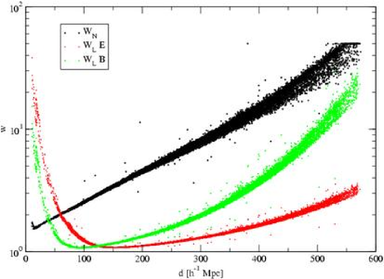
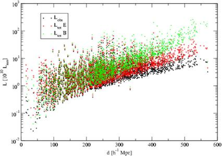
Figure 1.: The left panel shows the weights for observed galaxies, which are used to correct for invisible galaxies outside the observational window. Black symbols show the number-density weights, green and red symbols show the luminous-density weights, using the Blanton and Einasto sets of the Schechter function parameters, respectively. In the right panel we plot luminosities of galaxies: black symbols show observed luminosities, and green and red symbols show total luminosities for the Blanton and Einasto sets of the Schechter function parameters.

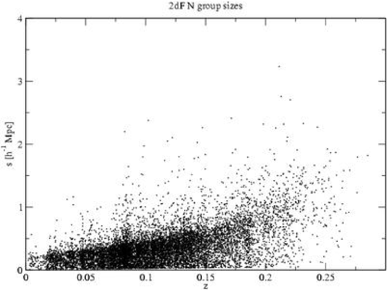
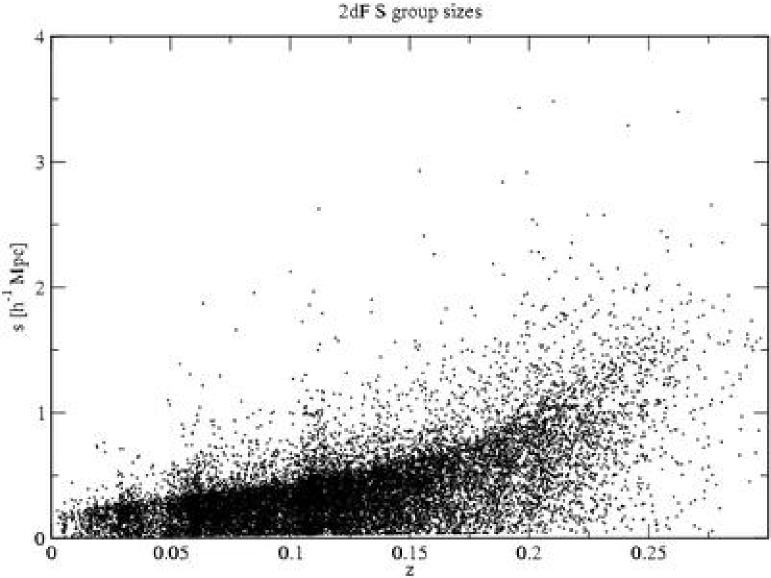
Figure 2.: Sizes of groups in the 2dF survey as found by Eke et al. eke04 (2004) as a function of their redshift $z$. The left panel shows the groups in the Northern Galactic hemisphere, the right panel shows the groups in the Southern hemisphere.

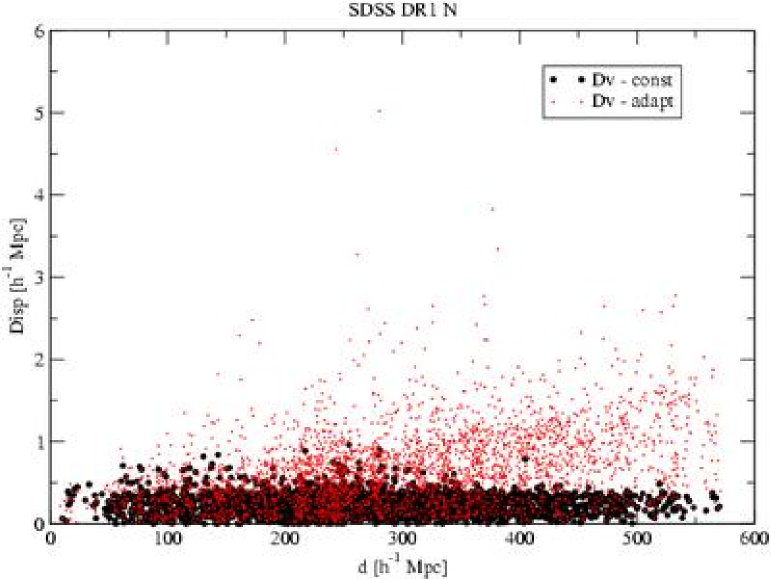
Figure 3.: The virial radii of groups(clusters) of galaxies in the Northern hemisphere, found with a constant (black dots) and a variable (red crosses) search radius.

3. Data reduction

Our data reduction procedure consists of several steps: (1) calculation of the distance, the absolute magnitude, and the weight factor for each galaxy of the sample; (2) finding groups/clusters of galaxies using the friends-of-friends algorithm; (3) calculation of the density field using an appropriate kernel and a selected smoothing length. When calculating luminosities of galaxies, we regard every galaxy as a visible member of a density enhancement (group or cluster) within the visible range of absolute magnitudes, $M_{1}$ and $M_{2}$, corresponding to the observational window of apparent magnitudes at the distance of the galaxy. This assumption is based on observations of nearby galaxies, which indicate that practically all galaxies belong to poor groups, like our own Galaxy, where one bright galaxy is surrounded by a number of faint satellites. Using this assumption we find halos, either halos of single giant galaxies with their companions, or halos of groups/clusters. Further, we assume that the luminosity function derived for a representative volume can be applied also for individual groups and galaxies.

Figure 4.: An example of an observed complex of galaxies (in equatorial coordinates), collected to a group using a variable search radius (open and filled circles), and a constant search radius (filled circles only). The group found with a variable search radius (DR1 199) consists of a cluster of galaxies, A933=DR1 244, and of a group DR1 202, embedded in a cloud of loosely located galaxies.

Calculation of distances, absolute magnitudes and weight factors for galaxies has been described in detail in E03a. In order to derive total luminosities of galaxies from their observed luminosities, we applied the Schechter S76 (1976) function with two sets of parameters. One set is based on the SDSS luminosity function by Blanton et al. blanton (2001), the other set on the SDSS luminosity function found in E03a, which yields better properties of clusters of galaxies; the respective values of the characteristic luminosity $M^{\ast}$ and the shape parameter $\alpha$ are given in Table 1. The subscripts B and E denote the parameter sets by Blanton et al. and Einasto et al., respectively.

In Fig. 1 we show the number-density and luminous-density weights as a function of distance. The number-density weight (shown here for comparison only) increases very rapidly with distance, showing the decrease of the number of galaxies in the observational window. The luminous-density weights based on the Blanton parameter set are rather large at large distances, the weights based on the Einasto set are much lower. The right panel of Fig. 1 shows the observed and total luminosities of galaxies at various distances. The total luminosities are corrected to account for galaxies outside of the observational window.

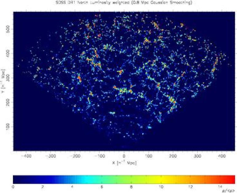
Figure 5.: The high-resolution density field of the Northern slice of SDSS DR1. The density was calculated using Gaussian smoothing with $\sigma=0.8$$h^{-1}$ Mpc. When calculating total luminosities of galaxies, the Schechter function parameters of the set E were used.

The next step is the search for groups and clusters of galaxies. Here we used the conventional friends-of-friends algorithm by Zeldovich, Einasto & Shandarin zes82 (1982) and Huchra & Geller hg82 (1982) (hereafter ZES and HG, respectively). These algorithms are essentially identical with one difference: ZES used a constant search radius to find neighbours whereas HG applied a variable search radius depending on the volume density of galaxies at a particular distance from the observer. The variant with a variable search radius is widely used, in particular by Eke et al. eke04 (2004), for constructing the group/cluster catalogue of 2dF redshift survey. To see how good this search algorithm is, we analyzed the mean radii of groups of this catalogue. The results of the analysis are shown in Fig. 2. We see that the sizes of groups, generated with a variable search radius, increase systematically with redshift $z$. Thus the population of such groups is not homogeneous, the groups at the far-away side of the sample are different from nearby groups.

For our group/cluster catalogue for SDSS DR1 we generated two versions, one with a constant search radius of 0.5 $h^{-1}$ Mpc, and the second with a variable search radius, which increased with distance proportionally to the mean distance between galaxies (as in HG). In both cases a radial linking length 500 km/s was used. The results are shown in Fig. 3. We see that the mean virial radii of groups/clusters are practically constant for the constant search radius case, and increase with distance for the variable search radius case. As an example, Fig. 4 shows the distribution of galaxies in the sky for one rich cluster. Using a variable search radius we include in the cluster two clusters of galaxies and a number of nearby field galaxies. One of these clusters is Abell 933; a constant search radius collects to the cluster galaxies inside a circle of radius 1.5 $h^{-1}$ Mpc, as used by Abell in his cluster catalogue. The second cluster is less rich and is not included in the Abell catalogue, its radius is also a bit smaller.

In the following analysis we have used only the group/cluster catalogue found with a constant search radius. The numbers of groups/clusters found for both equatorial slices are given in Table 1.

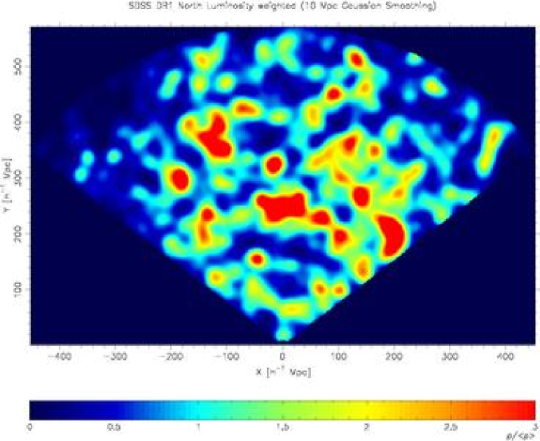
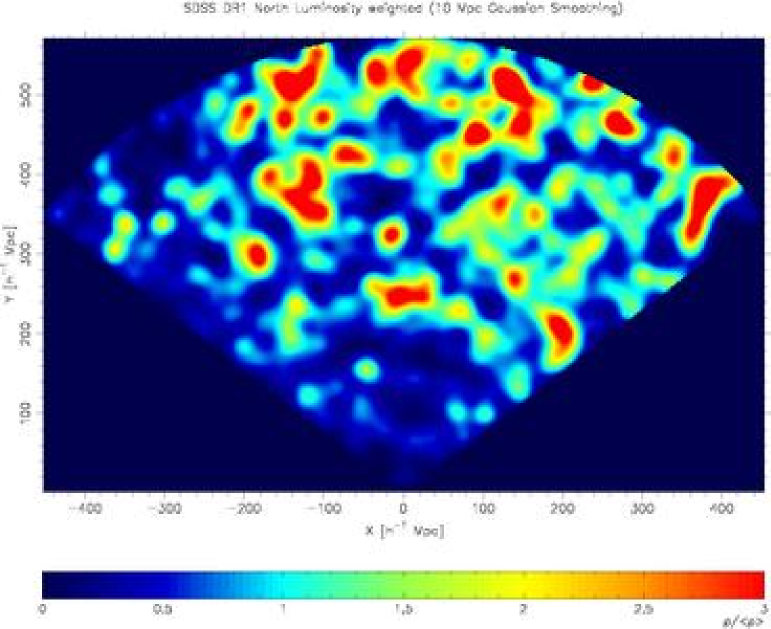
Figure 6.: The low-resolution luminosity density field of the Northern slice of SDSS DR1 (in units of the mean density). The density was calculated using Gaussian smoothing with $\sigma=10$$h^{-1}$ Mpc. The left panel shows the luminosity density for the set E of the Schechter function parameters, and the right panel – for the set B.

4. Density field

As both equatorial slices are very thin, we calculated only 2-dimensional luminosity density fields. As in E03a and E03b, we calculated the high-resolution density field using Gaussian smoothing with $\sigma=0.8$$h^{-1}$ Mpc, and the low-resolution field with $\sigma=10$$h^{-1}$ Mpc. The high-resolution field was found using the Schechter parameters of set E, and the low-resolution field with both parameter sets. The results are shown in Figs. 5 and 6, respectively. The low-resolution field was used to define superclusters as connected over-density regions. As in E03a, we used the density thresholds 1.8–2.1 to find superclusters. At lower thresholds superclusters start to merge into percolating systems, violating the definition of superclusters as largest but still isolated high-density regions. For higher thresholds the number of superclusters rapidly decreases (many of them have lower peak density).

The comparison of high- and low-resolution fields yields information on the fine structure of superclusters of various size and luminosity. We see that within superclusters clusters may form a single filament, a branching system of filaments, or a more or less diffuse cloud of clusters. Also we see that clusters themselves have various richness: in massive superclusters most clusters are very bright, in poor superclusters galaxy systems are also poor.

Fig. 6 shows that the mean luminosity of superclusters found for the set B of the Schechter parameters increases considerably with distance. In other words, this parameter set gives too high weights for galaxies outside the visibility window. In contrast, the parameter set E yields superclusters that are a bit too luminous at medium distances from the observer. We note that the superclusters found by E03a and E03b for SDSS EDR and LCRS have luminosities which are, in the mean, independent of the distance from the observer. This shows that a very careful choice of the parameters of the Schechter function is essential. In the following analysis we used the parameter set E to find environmental densities for clusters of galaxies, as in this case the distance dependence of supercluster luminosities is much less than for the set B.

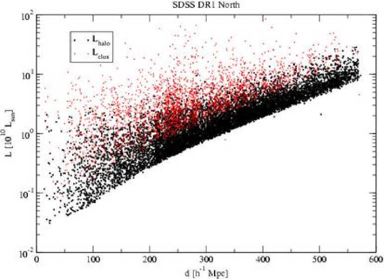
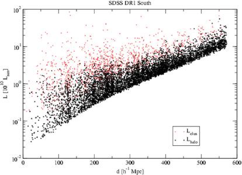
Figure 7.: Luminosities of groups/clusters at different distances, corrected for galaxies outside the visibility window. Red symbols denote groups with at least two visible galaxies, black symbols denote halos containing only one galaxy in the visibility window. The left panel shows the results for the SDSS Northern slice, the right panel – for the Southern slice.

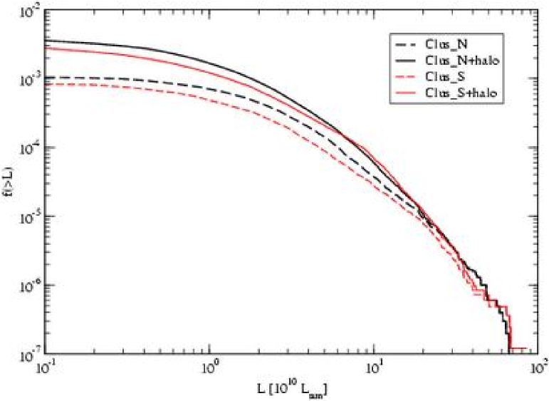
Figure 8.: Luminosity functions for SDSS DR1 groups/clusters. Dashed lines show functions found using clusters with at least two galaxies in the observational window, and solid lines show the luminosity functions for all groups/clusters, including halos with only one galaxy in the observational window. The set E of the Schechter function parameters was used to calculate total luminosities.

5. Properties of clusters and superclusters

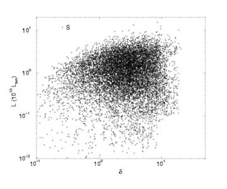
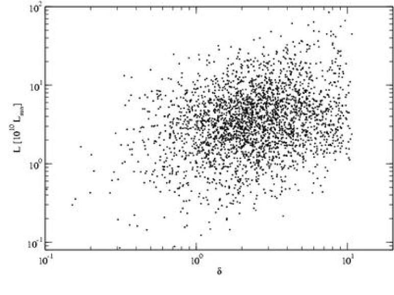
Figure 9.: The left panel shows the luminosities of galaxies in various density environments for the SDSS EDR Southern slice. The environmental density was calculated using Gaussian smoothing with $\sigma=2$$h^{-1}$ Mpc. The right panel shows the luminosities of the SDSS DR1 Northern slice clusters as a function of the environmental density, found with Gaussian smoothing of the luminous density field with $\sigma=10$$h^{-1}$ Mpc.

Fig. 7 shows luminosities of groups/clusters at different distances from the observer. We see that there exists a well-defined lower limit of cluster luminosities at larger distances; this limit is linear in the $\log L-d$ plot. Such behaviour is expected, as at large distances an increasing fraction of clusters does not contain any galaxies bright enough to fall into the observational window of absolute magnitudes, $M_{1}\dots M_{2}$. The limit is lower for groups containing only one galaxy in the visibility window; these groups are actually halos with one bright galaxy surrounded by faint companions. The low-luminosity limit for halos and groups containing at least two galaxies in the visibility window is two times higher, as expected (this factor corresponds to the case when both galaxies in the visibility window have equal luminosities).

Fig. 8 shows the integrated luminosity function of groups/clusters for the SDSS DR1 Northern and Southern samples. The absence of low-luminosity clusters at large distances has been taken into account by a standard weighting procedure (for details see E03a). The luminosity function was calculated separately for groups/clusters with at least two visible galaxies, and for all groups/clusters including halos with only one visible galaxy in the visibility window. In both cases the numbers of clusters have been corrected to take into account selection effects. Our calculations show that in the second case the number of groups/clusters per unit volume is larger for the low luminosity range of the luminosity function. This difference is probably due to the small number of low-luminosity groups.

The volume density of groups/clusters according to the SDSS DR1 data is $3\times 10^{-3}$ ($h^{-1}$ Mpc)^-3 for $L\geq 10^{9}$ $L_{\odot}$ groups/clusters. This estimate is in fairly good agreement with the estimates of the number density of groups based on the group mass function by Girardi & Giuricin gg00 (2000).

Let us now consider properties of galaxies and clusters in various environments. We shall use the density found with 2 $h^{-1}$ Mpc smoothing as an environmental parameter to describe the surrounding density of galaxies. Similarly, we use the density found with 10 $h^{-1}$ Mpc smoothing as the global density in the supercluster environment of clusters. The luminosity of galaxies as a function of the environmental density is shown in the left panel of Fig. 9. This Figure demonstrates the well-known density dependence of galaxies in systems: in groups and clusters the centrally located main galaxy has considerably higher luminosity than the surrounding galaxies.

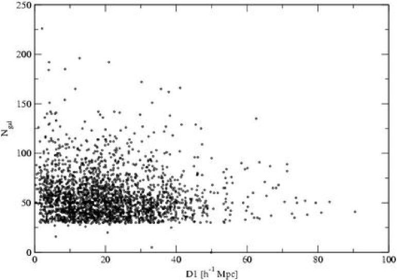
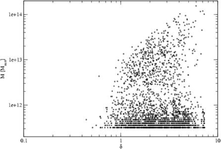
Figure 10.: The left panel shows Abell cluster richness (the number of galaxies in clusters) as a function of the distance to the 1st nearest neighbour, used as the environmental density parameter. The right panel shows masses of clusters in environments of various density in the N-body simulation. The density was found, using an Epanechnikov kernel with the radius 10 $h^{-1}$ Mpc.

On supercluster scales this effect is seen on the right panel of Fig. 9. There is a clear correlation between the luminosity of DF-clusters and their environmental density. Luminous clusters are predominantly located in high-density regions, and low-luminosity clusters – in low-density regions. This tendency can be seen also in Fig. 5. Here densities are color-coded, and we see that small clusters in voids have blue color, which indicates medium and small densities, whereas rich clusters having red color populate dominantly the central high-density regions of superclusters. For Abell clusters the dependence of the cluster richness on the density of the environment is shown on left panel of Fig. 10. The domination of faint galaxies in void regions was noticed by Lindner et al. l95 (1995). The environmental enhancement effect was found in the vicinity of rich clusters of galaxies by E03c and E03d.

6. Comparison with N-body models

The final step in our study is comparison of observational data with numerical simulations. We have used in this preliminary stage of the study a simulation with $128^{3}$ particles in a 100 $h^{-1}$ Mpc cube. Conventional cosmological parameters were used: the matter density $\Omega_{m}=0.3$, the dark energy density $\Omega_{\Lambda}=0.7$, the power spectrum amplitude parameter $\sigma_{8}=0.8$. Clusters were identified by the FoF algorithm with the search radius parameter $b=0.2$.

The mass of groups/clusters is plotted in the Fig. 10 as a function of the density of the environment, calculated with the Epanechnikov kernel 10 $h^{-1}$ Mpc. Here the dependence of the cluster mass on the density of the environment is very well expressed: most massive clusters in high-density environments have masses that are about two orders of magnitude higher than the masses of most massive clusters in low-density environments.

To understand better the dependence of cluster properties on the environment we studied the distribution of particle densities. We attributed to every particle in the simulation two density values, corresponding to the density at the location of the particle, found without smoothing and with smoothing. In the second case we used smoothing with the Epanechnikov kernel of a smoothing radius 10 $h^{-1}$ Mpc. This second density was used as a global environmental parameter. The whole simulation box was divided into 4 regions according to the global density $D$ (in units of the mean density): $D\geq 2$, $1\leq D<2$, $0.5\leq D<1$, and $D<0.5$. These global density regions correspond approximately to superclusters, rich and poor filaments, and systems in large voids. The results are shown in Fig. 11. We see that in superclusters (regions of high global density) the majority of particles are located in systems of high local density (rich clusters of galaxies). Further we see that a small fraction of particles is located in poor clusters or groups, and even a smaller fraction of particles form the void population. These particles have the local density less then 1 and cannot cluster, since galaxy formation starts only in the case if the local density exceeds a certain threshold, much higher than the mean density (see Press & Schechter ps74 (1974)). With a decreasing global density the fraction of particles in very rich clusters decreases, most particles belong to intermediate rich groups and clusters, and the fraction of particles in voids increases. Finally, in the void regions of the lowest global density most particles have local density less than 1, and a small fraction of particles are clustered forming very poor groups of galaxies (with local densities less than 10).

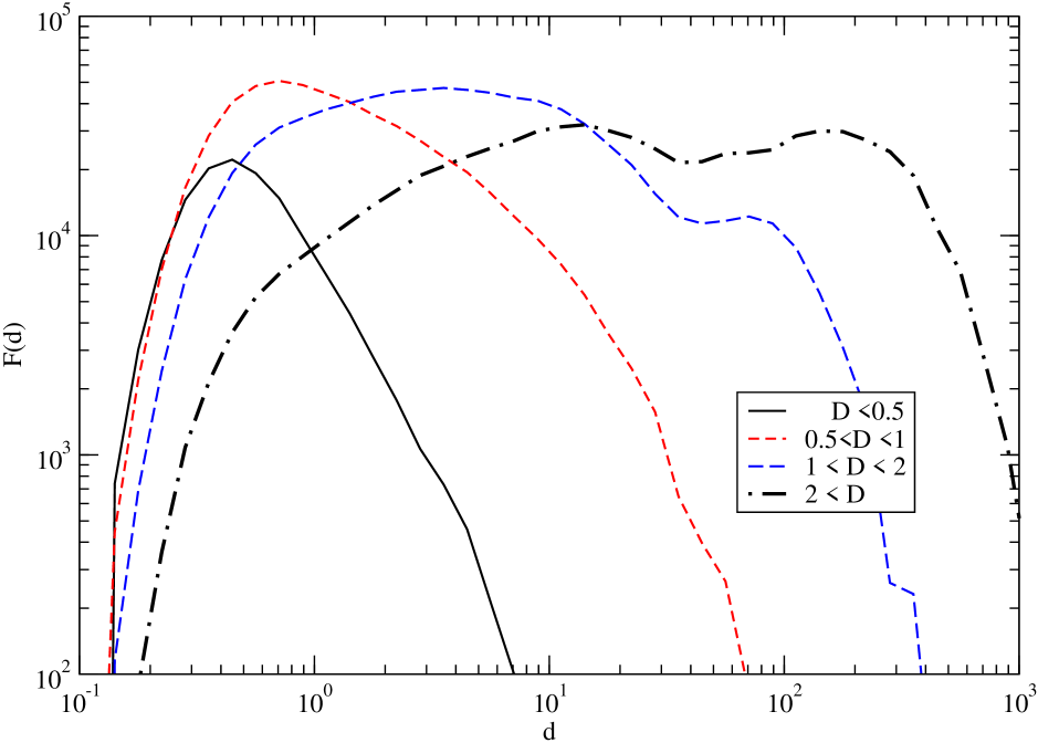
Figure 11.: The distribution of particles as a function of the local density $d$ of the environment in a N-body model. The local density of particles was found by interpolation of the unsmoothed density field. The distribution is shown for various regions of the global density $D$.

Differences in the evolution of high and low-density regions were studied by Frisch et al. f95 (1995), they are evident also in movies prepared by Gottlöber and Müller in the Potsdam Astrophysical Institute. One movie was made for a high-density region (the central cluster of a rich supercluster), the other movie for a large under-dense region of 20 $h^{-1}$ Mpc diameter (in co-moving coordinates). In the high-density region the galaxy formation starts at an early epoch and leads to a rapid merging of numerous small clumps to a very rich cluster. In the large void region a filamentary network of clustered particles also forms, but these filaments are relatively poor and contain only a small number of knots which can be identified with dwarf galaxies and very poor groups.

Finally we used numerical simulations to investigate properties of superclusters. In addition to the density fields derived with two different smoothing lengths we calculated also the gravitational potential field with and without smoothing. In the unsmoothed potential field all clusters of galaxies are seen as local attractors, which distort the otherwise smooth potential field. Rich superclusters can be identified as large depressions in the potential field. However, in contrast to the density field derived with a large smoothing length, it was impossible to define low-mass superclusters using the potential field. The reason is simple – the potential field is much shallower than the density field, and low-mass superclusters do not generate a depression in the potential field deep enough to make the identification of the supercluster possible.

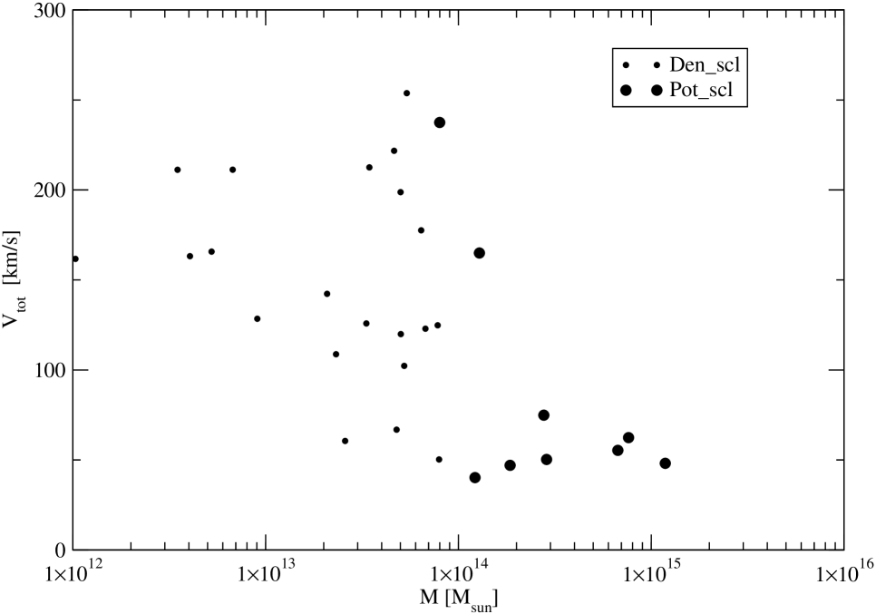
Figure 12.: The mean total velocity of superclusters in a N-body simulation as a function of their mass (in Solar mass units). Large symbols denote for superclusters which can be identified both in the gravitational potential as well as in the smoothed density field, small symbols denote superclusters which were found only in the density field.

To find superclusters in a simulation we applied the same procedure as for real superclusters, i.e. they were identified as relatively isolated high-density regions in the low-resolution density field. Experimentation with various threshold density levels showed that the optimal density level to extract superclusters lies in the interval $1.8\dots 2.1$ (in units of the mean density). Similar threshold densities were also applied to find real superclusters in both the SDSS and LCRS galaxy samples by E03a and E03b. We calculated masses of superclusters by adding masses of clusters within supercluster boundaries. Next we calculated mean velocities of superclusters by summing up velocities of all clusters in superclusters. These velocities as a function of supercluster mass are shown in Fig. 12. In this figure, massive superclusters which can be identified both in the density, as well as in the potential field, are plotted by large symbols. We see that these massive superclusters have low bulk velocities, and there is a rather sharp transition to less massive superclusters, which have much larger bulk velocities. In other words, massive superclusters can be considered great attractors, whereas low-mass superclusters are much smaller attractors. Presently this phenomenon has been established only in a relatively small simulation box.

To conclude we can say that the study of clusters in the SDSS DR1 using 3-dimensional information has confirmed our preliminary results based on the SDSS EDR and LCRS on the environmental dependence of cluster properties. Numerical simulations show that in large underdense regions most particles form a rarefied population of pregalactic matter whereas in large overdense regions most particles form a clustered population in rich clusters. Comparison of observational data with results of numerical simulation shows that superclusters can be divided into two classes; very massive superclusters are great attractors, low-mass superclusters are small attractors having larger bulk velocities.

References

- (1) Abell, G., 1958, ApJS, 3, 211
- (2) Abell, G., Corwin, H. & Olowin, R., 1989, ApJS, 70, 1
- (3) Andernach, H. & Tago, E., 1998, in Large Scale Structure: Tracks and Traces, eds. V. Müller, S. Gottlöber, J.P. Mücket & J. Wambsganss, World Scientific, Singapore, p. 147
- (4) Bahcall, N., 1988, ARA&A, 26, 631
- (5) Basilakos, S., 2003, MNRAS, 344, 602
- (6) Blanton, M. R., Dalcanton, J., Eisenstein, D. et al. 2001, AJ, 121, 2358
- (7) Einasto, J., Einasto, M., Hütsi, G., Saar, E., Tucker, D. L., Tago, E., Müller, V., Heinämäki, P., & Allam, S. S., 2003a, A&A, 410, 425, (E03a)
- (8) Einasto, J., Hütsi, G., Einasto, M., Saar, E., Tucker, D. L., Müller, V., Heinämäki, P., & Allam, S. S., 2003b, A&A, 405, 425, (E03b)
- (9) Einasto, M., Einasto, J., Tago, E., Dalton, G. & Andernach, H., 1994, MNRAS, 269, 301 (E94)
- (10) Einasto, M., Einasto, J., Tago, E., Müller, V. & Andernach, H., 2001, AJ, 122, 2222 (E01)
- (11) Einasto M., Einasto J., Müller, V., Heinämäki, P.,& Tucker, D. L., 2003c, A&A, 401, 851, (E03c)
- (12) Einasto M., Jaaniste, J., Einasto J., Heinämäki, P., Müller, V., & Tucker, D. L., 2003d, A&A, 405, 821, (E03d)
- (13) Einasto, M., Tago, E., Jaaniste, J., Einasto, J. & Andernach, H., 1997, A&A Suppl., 123, 119 (E97)
- (14) Eke, V. R., Baugh, C. M., Cole, S., et al., 2004, astro-ph/0402567
- (15) Frisch, P., Einasto, J., Einasto, M., Freudling, W., Fricke, K. J., Gramann, M., Saar, V. & Toomet, O., 1995, å, 296, 611
- (16) Girardi, M., & Giuricin, G., 2000, ApJ, 540, 45
- (17) Heinämäki, P., Einasto, J., Einasto, M., Saar, E., Tucker, D. L., & Müller, V., 2003, A&A, 397, 63
- (18) Huchra, J. P., & Geller, M. J., ApJ, 257, 423
- (19) Lindner, U., Einasto, J., Einasto, M., Freudling, W., Fricke, K.,& Tago, E., 1995, A&A, 301, 329
- (20) Oort, J.H., 1983, ARAA, 21, 373
- (21) Press, W.H. & Schechter, P.L., 1974, ApJ, 187, 425
- (22) Schechter, P., 1976, ApJ, 203, 297
- (23) Tucker, D.L., Oemler, A.Jr., Hashimoto, Y., Shectman, A., Kirshner, R.P., Lin, H., Landy, S.D., Schechter, P.L.,& Allam, S.S., 2000, ApJS, 130, 237
- (24) Zeldovich, Ya.B., Einasto, J. & Shandarin, S.F. 1982, Nature, 300, 407
- 1961– (68) Zwicky, F., Wield, P., Herzog, E., Karpowicz, M. & Kowal, C.T. 1961–68, Catalogue of Galaxies and Clusters of Galaxies, 6 volumes. Pasadena, California Inst. Techn.