A Homogenous Set of Globular Cluster Relative Distances and Reddenings

We present distance modulus and reddening determinations for 72 Galactic globular clusters from the homogeneous photometric database of Piotto et al. (2002), calibrated to the HST flight F439W and F555W bands. The distances have been determined by comparison with theoretical absolute magnitudes of the ZAHB. For low and intermediate metallicity clusters, we have estimated the apparent Zero Age Horizontal Branch (ZAHB) magnitude from the RR Lyrae level. For metal rich clusters, the ZAHB magnitude was obtained from the fainter envelope of the red HB. Reddenings have been estimated by comparison of the HST colour-magnitude diagrams (CMD) with ground CMDs of low reddening template clusters. The homogeneity of both the photometric data and the adopted methodological approach allowed us to obtain highly accurate relative cluster distances and reddenings. Our results are also compared with recent compilations in the literature.

1 Introduction

Galactic Globular Clusters (GGCs) are extremely useful astronomical probes. Because they are the oldest objects for which we can estimate the age, GGCs are commonly used to infer relevant information on both the Galaxy formation timescale and the early Universe. Moreover, they constitute a well suited laboratory to study both the evolution of low-mass stars, and stellar dynamics.

Two key parameters needed in GGC studies are their distances and reddenings. As an example, the use of the absolute magnitude of turnoff stars in the cluster colour-magnitude-diagram (CMD) to determine the cluster age (see, e.g. Vandenberg, Stetson & Bolte 1996; Salaris & Weiss 1998, and references therein) needs an accurate distance estimate. Also, the comparison between various observed features of their CMDs (e.g., the absolute magnitude of the luminosity function red giant branch bump, or the level of the tip of the red giant branch) and the theoretical counterparts does require a preliminar knowledge of both the cluster reddening and the distance.

A definitive assessment of both the absolute and relative GGC distance scale is still lacking, mostly due to the fact that the ’traditional’ Population II standard candle, e.g. the brightness of RR Lyrae pulsating stars, is not yet reliably calibrated empirically (e.g. Cacciari 2003). This is partially due to the paucity of RR Lyrae stars in the solar neighbourhood, and the consequent large errors in RR Lyrae parallax determinations, even for the recent $Hipparcos$ data (Groenewegen & Salaris 1999), and also to the existence of significant systematic and random uncertainties in other less direct methods applied to determine the RR Lyrae intrinsic brightness (Bono 2003).

The advent of $Hipparcos$ parallaxes has on the other hand improved the accuracy of the GGC distance determination by the subdwarf Main Sequence (MS) fitting technique (e.g.. Carretta et al. 2000). The problem here is that this method can be reliably applied only to a handful of low reddening clusters, with deep and well calibrated high accuracy MS photometry; in addition, current uncertainties on the metallicity scale of both clusters and subdwarfs, and on the cluster reddenings may still cause sizable uncertainties on the distances derived by means of this method (compare, e.g., the results by Carretta et al. 2000 with Reid 1997, 1998).

In order to assess the accuracy and reliability of the various methods used to infer GGC distances, it is important to compare the distance measurements obtained with as many as possible different and independent distance indicators, such as the aforementioned empirical MS fitting, the RR Lyrae method, and the fitting of theoretical Horizontal Branch (HB) models to their observational counterpart. This kind of comparison is relevant not only for checking the consistency between the various distance indicators, but also for verifying the reliability of the adopted, if any, theoretical scenario, as in the case of distances based on the fit to HB models. On this respect, we note that a database of relative distances and reddenings is of extreme importance: once we have accurate absolute distances and reddenings for a set of GGCs, this database can be easily used to obtain the absolute values for all the other clusters.

In the last decade, we have been working on a long-term project aimed at carrying out a detailed quantitative analysis of the various evolutionary sequences in the CMD of GGCs. Our main goals include the derivation of an accurate GGC relative age scale (Rosenberg et al. 1999, Piotto et al. 2000), and a test of the accuracy of theoretical models for low-mass metal-poor stars. The main body of this investigation has been performed by adopting an homogeneous and self-consistent photometric dataset (available at http://dipastro.pd.astro.it/globulars), based on both ground based observations (Rosenberg et al 2000a, 2000b), and Hubble Space Telescope data (the HST snapshot catalogue: Piotto et al. 2002). This large observational database has also been used to investigate the level of agreement between theory and observations concerning evolutionary timescales (Zoccali and Piotto 2000), the brightness and size of the luminosity function Red Giant Branch (RGB) bump (Zoccali et al. z99 (1999); Bono et al. 2001; Riello et al. 2003), the mixing length parameter (Palmieri et al. 2002), the initial helium content (Zoccali et al. 2000; Cassisi et al. 2003; Salaris et al. 2004), the HB morphology (Piotto et al. 1999), the blue straggler stellar population (Piotto et al. 2004). The majority of these works needed an as accurate as possible distance and reddening determination, and in most cases we used a new set of distances and reddenings, based on our photometrically homogeneous HST snapshot database. In this paper we present and thoroughly discuss how we obtained the distances and reddenings adopted in the works above mentioned.

Distance estimates have been obtained from the fitting of theoretical HB models to the observed counterpart in the CMD. We accurately measured the observed HB luminosity level and, in turn, the distance modulus, for about 40% of the total GGC population, covering most of the GGC metallicity range. Our relative distances and reddenings are more accurate than previous compilations, because they are based on a homogeneous photometric database, and have been derived by applying consistently the same technique to all clusters. Moreover, the theoretical HB models we employed (Pietrinferni et al. 2004) have been computed accounting for the most updated input physics.

The plan of the paper is as follows: in Section 2, we describe briefly the photometric database and the theoretical models. Section 3 presents the actual measurements and the values of the distance moduli. We compare our distance estimates with relevant data available in the literature in Section 4 and, finally, the main conclusions are summarized in Section 5.

2 The observational and theoretical databases

2.1 The cluster database

The distance determinations presented here are based on the large photometric data set from Piotto et al. (2002), observed with HST in the F439W and F555W bands, calibrated to the WFPC2 flight system. The complete database includes a total of 74 GGCs, and represents an unique opportunity to measure fundamental parameters of GGCs.

The observations, preprocessing, photometric reduction, and calibration of the instrumental magnitudes to the HST flight system, as well as the artificial star experiments performed to derive the star count completeness, are reported in full details in Piotto et al. (2002). For the purpose of this paper, we point out that all the data have been processed following the same reduction steps: after the pre-processing, the instrumental photometry for each cluster was obtained with DAOPHOT II/ALLFRAME (Stetson, 1987; Stetson, 1994), the correction for the CTE effect and the calibration to the flight system was accomplished following the prescriptions by Dolphin (2000).

2.2 The GGCs metallicity scale

One of the pivotal problems in estimating both distances and ages for GGCs is the adopted metallicity scale. As recently stated by Rutledge, Hesser & Stetson (1997, see also VandenBerg v00 (2000); Caputo & Cassisi cc02 (2002) and Kraft & Ivans ki03 (2003)) current estimates of the [Fe/H] values for GGCs are affected by an uncertainty of the order of at least 0.15 dex. The situation becomes even more uncertain when we consider the $\alpha-$element enhancement in GGC stars: the measurements of $\alpha-$elements are affected by both random and systematic uncertainties, they have been obtained in an heterogeneous way, and only for a very limited number of GGCs.

In order to properly account for these unavoidable drawbacks we decided, as in our previous works, to adopt the two most widely used scales for the metal abundance in GGCs: the Zinn & West (1984) scale (hereinafter ZW), and the Carretta & Gratton (1997, hereinafter CG) one. As for the $\alpha-$element enhancement, due to the lack of self-consistent and accurate measurements for a sizeable sample of GGCs, we adopt the following assumption: a mean [$\alpha$/Fe]=0.3 dex for metal-poor and metal-intermediate clusters $(\mathrm{[Fe/H]}<-1.0)$, and [$\alpha$/Fe]=0.2 dex for metal-rich clusters $(\mathrm{[Fe/H]}\geq-1.0)$. The choice of the former value is based on the estimates provided by Carney (carney (1996)), while the latter is obtained as a mean between the values collected by Carney (carney (1996)) and by Salaris & Cassisi (sc96 (1996)).

In order to estimate the global cluster metallicity by accounting for the proper [Fe/H] value, and the chosen $\alpha-$element enhancement, we have adopted the prescriptions provided by Salaris, Chieffi & Straniero (scs93 (1993)), i.e.:

[M/H] $=[Fe/H]+log(0.638f+0.362)$ ; $\log{f}=[\alpha/Fe]$

We assume an uncertainty of the order of $\pm$ 0.15 dex on [M/H], which accounts for the uncertainties on both $\mathrm{[Fe/H]}$ and $[\alpha/\mathrm{Fe}]$ measurements (Rutledge et al. 1997).

2.3 The theoretical framework

The theoretical predictions adopted in this investigation are based on the updated set of stellar models by Pietrinferni et al. (2004), and we refer the interested reader to that paper for a complete discussion about these models. For the purposes of this paper, we briefly list the main changes in the adopted physical inputs with respect to previous works (Cassisi & Salaris 1997):

• the radiative opacity is obtained from the OPAL tables (Iglesias & Rogers 1996) for temperatures larger than $10^{4}$ K, and from Alexander & Ferguson (alexander (1994)) for lower temperatures. Conductive opacity for electron degenerate matter is computed following Potekhin (pot (1999)).

• We updated the energy loss rates for plasma-neutrino processes by using the most recent and accurate results provided by Haft, Raffelt & Weiss (haft (1994)). For all other processes we still rely on the same prescriptions adopted by Cassisi & Salaris (1997).

• The nuclear reaction rates have been updated by using the NACRE database (Angulo et al. 1999), with the exception of the ¹²C$(\alpha,\gamma)^{16}$O reaction. For this reaction we now adopt the more accurate recent determination by Kunz et al. (kunz (2002)).

• The accurate Equation of State (EOS) by A. Irwin has been used. An exhaustive description of this EOS is still in preparation (Irwin et al. 2004) but a brief discussion of its main characteristics can be found in Cassisi, Salaris & Irwin (csi03 (2003)). It is enough to mention here that this EOS, whose accuracy and reliability is similar to the OPAL EOS developed at the Livermore Laboratories (Rogers, Swenson & Iglesias rsi96 (1996)) and recently updated in the treatment of some physical inputs (Rogers & Nayfonov rn02 (2002)), allows us to compute self-consistent stellar models in all evolutionary phases relevant to present investigation.

• The extension of the convective zones is fixed by means of the classical Schwarzschild criterion. Induced overshooting and semiconvection during the He-central burning phase are accounted for following Castellani et al. (cast85 (1985)). The thermal gradient in the superadiabatic regions is determined according to the mixing length theory, whose free parameter has been calibrated by computing a solar standard model.

• The set of evolutionary models has been computed for metallicities in the range: $0.0001\leq{Z}\leq 0.04$. However, in the present work only the models for metallicity equal or lower than the solar one have been used. We adopt the scaled-solar heavy element mixture (Grevesse & Noels gn93 (1993)).

• As far as the initial He-abundance is concerned, we adopt the estimate recently provided by Salaris et al. (s04 (2004)) on the basis of new measurements of the $R$ parameter in a large sample of GGCs. They found an initial He-abundance for GGC stars of the order of $Y=0.245$, which is in fair agreement with recent empirical measurements of the cosmological baryon density provided by W-MAP (Spergel et al. 2003). To reproduce the calibrated initial solar He-abundance we used $dY/dZ\approx 1.4$ (Pietrinferni et al. 2004).

• For each fixed chemical composition, we have adopted the He core mass and the surface He abundance at the RGB tip of a star igniting central He burning at an age of about $\sim 12$ Gyr. Once the RGB progenitor mass is chosen, a suitable set of Zero Age Horizontal Branch (ZAHB) models for different assumptions about the mass of the H-rich stellar envelope – i.e., about the efficiency of mass loss during the RGB phase – has been computed. In brief, the initial models of our HB sequences have a fully homogeneous H-rich envelope around the He core mass of the selected progenitor; the proper ZAHB model is obtained when all the secondary elements involved in the H-burning through the CNO-cycle are relaxed to their equilibrium values.

• Bolometric magnitudes have been transformed to HST F555W magnitudes according to the transformations provided by Origlia & Leitherer (origlia (2000)), which based on the atmosphere models computed by Bessell, Castelli & Plez (bcp98 (1998)).

From the computed ZAHB models, we have estimated the ZAHB brightness at the level of the RR Lyrae instability strip, i.e., at $\log{T_{e}}\approx 3.85$. In Table 1 we list, for each assumed chemical composition, the bolometric magnitude, the star mass and the HST F555W magnitude of the ZAHB at $\log{T_{e}}=3.85$.

By performing a quadratic regression to these data, we obtain the following dependence of the ZAHB F555W magnitude on the stellar total metallicity:

M${}^{ZAHB}_{F555W}=0.981+0.410[M/H]+0.061[M/H]^{2}$       1)

with $r^{2}=0.99$, which is valid in the metallicity range: $-2.3\leq[M/H]\leq 0.06$.

The models adopted in this work have been computed by neglecting atomic diffusion. However, Castellani et al. (1997) and Cassisi et al. (1998) have shown that the effect of atomic diffusion on the ZAHB brightness at the level of the RR Lyrae instability strip is to decrease it of about $\Delta{\log}(L/L_{\odot})\approx 0.02$, i.e., $\Delta{F555W}\approx+0.05$ mag. This means that, if we would account for the occurrence of atomic diffusion, the derived distance modulus estimates (see next section) would be decreased only by about 0.05 mag.

As stated above, our theoretical ZAHB luminosities are based on updated stellar models, computed by accounting for the ‘best’ physics presently available. However we are aware of remaining uncertainties affecting the prediction of the HB brightness, as discussed by several authors (Vandenberg et al. 2000, De Santis & Cassisi 1999, Cassisi et al. 1998 and references therein). We refer the reader to the quoted papers for deeper analysis on this subject. Here we will compare the distances obtained using our ZAHB models with independent empirical determinations, in order to test the accuracy of the models we employed.

Table 1: Theoretical predictions for the ZAHB luminosity, evolutionary mass and absolute F555W magnitude at the RR Lyrae instability strip as a function of $[M/H]$.

$[M/H]$	$M/M_{\odot}$	$\log(L/L_{\odot})$	F555W (mag)
-2.27	0.821	1.780	0.351
-1.79	0.721	1.732	0.468
-1.27	0.650	1.687	0.564
-0.96	0.620	1.653	0.634
-0.66	0.594	1.614	0.721
-0.25	0.565	1.540	0.884
0.06	0.543	1.489	0.988

3 Distance moduli determination

The distance modulus for each cluster in the database was obtained by comparing the F555W apparent ZAHB magnitude with the theoretical absolute magnitude as obtained from equation 1). A standard method for deriving the ZAHB magnitude for both intermediate and metal-poor clusters is to adopt the mean magnitude of the corresponding RR Lyrae stars. This however was not possible in our case because the Piotto et al. (2002) photometry covers a very short time interval and, as a consequence, the RR Lyrae stars were always measured at random pulsation phases.

In order to overcome this problem, we have undertaken an approach similar to the one already used by Zoccali et al. (1999). We first divided the clusters into two samples on the basis of their metallicity: the low- and intermediate-metallicity (hereinafter LIM) clusters ($[Fe/H]<-1.0$), and the metal-rich (hereinafter MR) clusters ($[Fe/H]\geq-1.0$). In the following, we describe in details the different approaches we used to estimate the ZAHB level for the two different cluster samples.

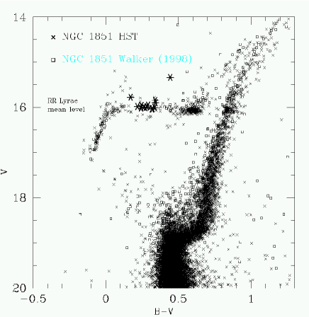
Figure 1: Comparison between the ground-based CMD of NGC1851 obtained by Walker (1998) and the HST CMD one, transformed to the standard Johnson system. The location of the RR Lyrae stars as observed by Walker (1998) is also shown (asterisks). The horizontal line displays the mean RR Lyrae luminosity level.

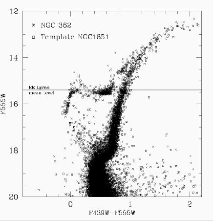
Figure 2: Determination of the mean RR Lyrae F555W magnitude in the cluster NGC362 by comparing its CMD with the template CMD of NGC1851. The horizontal line displays the estimated mean RR Lyrae magnitude.

3.1 The ZAHB luminosity level for LIM clusters

Since the HB morphology does strongly depend on the cluster metallicity, we selected five clusters, all with metallicity lower than – or approximately equal to – [Fe/H]=$-1.0$, to use as template clusters. They have been selected according to the following prescriptions:

• low interstellar reddening;

• a sizeable population of RR Lyrae variables;

• accurate ground-based photometric data for both static and pulsating stars.

The selected clusters are NGC 1851( Walker, 1998), NGC 4590 (Walker 1994), NGC 5272 (Buonanno et al. 1994), NGC 5904 (Caputo et al. 1999) and NGC 6362 (Walker 2001, priv. com.).

By using the histogram of the observed RR Lyrae mean magnitudes, we estimated the mean RR Lyrae luminosity level in the standard Johnson system, for all the five clusters selected from the literature. These clusters will be used to determine the ZAHB level in other GGCs, that cannot fulfill all three conditions listed before, within a narrow metallicity range around the template ones.

The metallicity of the templates on the ZW scale, the [Fe/H] range within which they have been employed, and the mean $V$ and $F555W$ magnitudes of their RR Lyrae stars are listed in Table 2.

We took care that all the selected template clusters had a reddening E($B-V$)$<$0.1, in order to minimize calibration errors in the determination of the RR Lyrae level when comparing the ground-based CMDs with the HST snapshot ones transferred in the Johnson system (see below).

The method for estimating the ZAHB luminosity level in the F555W HST band, adopted for all LIM clusters, is the following:

• the mean RR Lyrae luminosity level in the ground-based Johnson system for the template clusters has been translated into the HST flight photometric system. Due to the fact that there are non-negligible differences between the standard ground-based Johnson photometry and the HST flight photometry, this has been accomplished following a two-step procedure. As a first step, we have superposed the ground-based CMD to the corresponding HST snapshot CMD calibrated to the Johnson system. This has allowed us to set the RR Lyrae mean magnitude measured on the groundbased CMD on the HST snapshot CMD. After this, we have transferred the RR Lyrae mean level to the CMD in the WFPC2 flight system. This allowed us to measure the RR Lyreae mean $F555W$ magnitude in the WFPC2 flight system. The mean apparent magnitude of the template cluster RR Lyrae stars has been then transformed into the apparent ZAHB magnitude by accounting for the formula by Cassisi & Salaris (1996). The use of this relation is particularly justified by the fact that all the template clusters have a sizeable population of RR Lyraes stars.

  m${}^{ZAHB}_{F555W}=m^{RR-Lyrae}_{F555W}+0.152+0.041[M/H]$

  NGC 5272, was not included in the Piotto et al. (2002) database. For that reason, we overlapped its CMD to the snapshot CMD of NGC 1904 ([Fe/H]=$-1.6$) in order to fix the RR Lyrae level, and then adopted the snapshot CMD of NGC 1904 as template to determine the ZAHB level of the clusters in the corresponding (see table. 2) metallicity interval.

• the ZAHB $F555W$ magnitude for each remaining cluster in our sample has been determined in the following way. The appropriate template HST snapshot CMD calibrated to the flight system has been shifted in both magnitude and colour over the CMD of the cluster, until their HBs overlap, as illustrated in Fig. 2. In particular, we have been careful to match the region of the blue HBs around the point where the HB becomes vertical in the ($F555W$, $F439W-F555W$) plane. The location of this point on the CMD depends only on the bolometric correction, and is independent on metallicity (Brocato et al.  1998). This procedure allowed us to obtain both the m${}^{ZAHB}_{F555W}$ magnitude and the E($F439W-F555W$) reddening relative to the template one.

Table 2: Cluster templates for the measurement of the average RR Lyrae level. The estimated error in the mean RR Lyrae F555W magnitude is of the order of 0.05 mag.

Cluster	[Fe/H]	metallicity range	$<V(RR)>$	$<F555W(RR)>$
NGC 6362	$-1.1$	$-$1.1$<$[Fe/H]$<-$0.8	15.29	15.30
NGC 1851	$-1.2$	$-$1.3$<$[Fe/H]$\leq-$1.1	16.04	16.04
NGC 5904	$-1.4$	$-$1.5$<$[Fe/H]$\leq-$1.3	15.07	15.10
NGC 1904	$-1.7$	$-$1.8$<$[Fe/H]$\leq-$1.5	16.17	16.16
NGC 4590	$-2.1$	[Fe/H]$\leq-1.8$	15.58	15.65

Figure 3: Determination of F555W magnitude of the ZAHB for the metal-rich cluster NGC 104. Left panel: the HST CMD of the cluster. Right panel: the histogram of the stellar cluster population within the box shown in the left panel.

3.2 High metallicity clusters

For clusters with [Fe/H] $\geq$ -1.0, showing generally a red HB and no RR Lyrae stars, the magnitude m${}^{ZAHB}_{F555W}$ was derived according to the following relation (see Zoccali et al. (1999) for more details):

m${}^{ZAHB}_{F555W}=m^{le}_{F555W}-3\sigma_{F555W}$

where m${}^{le}_{F555W}$ is the magnitude of the lower (fainter) envelope of the red HB, previously determined on the histogram of the magnitude distribution of the HB stars, as shown in Figure 3, and $\sigma_{F555W}$ is the photometric error at the HB magnitude interval, estimated through artificial star experiments. In general, $\sigma_{F555W}$ is of the order of 0.02 mag, representing very small deviations in magnitude. Where possible (i.e. for clusters with a red HB, but a metallicity low enough to be able to determine the RR Lyrae level by comparison with the template clusters), we have verified that the two methods give consistent ZAHB magnitudes.

The final apparent distance moduli for all our clusters were calculated by simply computing the difference (m${}^{ZAHB}_{F555W}$ - M${}^{ZAHB}_{F555W}$), where the absolute ZAHB magnitudes were obtained from Eq. 1. Tables 3 and 4 list the distance moduli and reddenings obtained for our data set. Note that, due to the CMD photometry accuracy, we could measure the distance to 72 out of the 74 clusters in the snapshot sample. For 2 clusters, field star contamination and/or differential reddening made impossible to measure the ZAHB magnitude.

ID	m(ZAHB)	(m-M)	Reddening	E(B-V)	[Fe/H]	[Fe/H]
	$F555W$	$F555W$			ZW	CG
ic1257	20.20	19.69$\pm$0.10	0.71	0.72	…….	……
ic4499	17.75	17.22$\pm$0.10	0.15	0.15	-1.5	-1.29
n0104	14.16	13.41$\pm$0.08	…….	…….	-0.71	-0.70
n0362	15.50	14.85$\pm$0.10	0.005	0.004	-1.27	-1.15
n1261	16.85	16.26$\pm$0.09	0.01	0.01	-1.31	-1.17
n1851	16.15	15.52$\pm$0.10	0.02	0.02	-1.36	-1.20
n1904	16.25	15.71$\pm$0.08	0.01	0.01	-1.69	-1.37
n2808	16.35	15.70$\pm$0.09	0.14	0.14	-1.37	-1.21
n3201	14.85	14.32$\pm$0.08	0.24	0.25	-1.61	-1.23
n4590	15.73	15.30$\pm$0.08	0.05	0.05	-2.09	-1.99
n4147	16.98	16.50$\pm$0.08	0.01	0.01	-1.80	-1.55
n4372	15.58	15.15$\pm$0.09	0.40	0.42	-2.08	-1.93
n4833	15.70	15.21$\pm$0.08	0.28	0.29	-1.86	-1.58
n5024	16.83	16.38$\pm$0.08	0.01	0.01	-2.04	-1.86
n5634	17.68	17.20$\pm$0.09	0.01	0.01	-1.82	-1.57
n5694	18.53	18.06$\pm$0.08	0.12	0.12	-1.92	-1.69
n5824	18.53	18.06$\pm$0.08	0.12	0.12	-1.87	-1.63
n5904	15.20	14.59$\pm$0.08	0.03	0.03	-1.40	-1.11
n5927	16.79	15.90$\pm$0.08	…….	…….	-0.30	-0.14
n5946	17.60	17.01$\pm$0.09	0.63	0.64	-1.37	-1.21
n5986	16.70	16.17$\pm$0.08	0.26	0.27	-1.67	-1.42
n6093	16.35	15.85$\pm$0.08	0.21	0.22	-1.68	-1.43
n6139	18.05	17.54$\pm$0.09	0.71	0.72	-1.65	-1.40
n6171	15.79	15.11$\pm$0.09	0.48	0.49	-0.99	-0.97
n6205	15.05	14.51$\pm$0.08	0.01	0.01	-1.65	-1.39
n6218	14.80	14.24$\pm$0.20	0.21	0.22	-1.61	-1.37
n6229	18.10	17.53$\pm$0.09	0.02	0.02	-1.54	-1.32
n6235	17.00	16.42$\pm$0.09	0.30	0.31	-1.40	-1.22
n6256	18.22	17.42$\pm$0.09	1.18	1.18	…….	…..
n6266	16.30	15.69$\pm$0.09	0.53	0.54	-1.28	-1.15
n6273	16.55	16.04$\pm$0.08	0.33	0.34	-1.68	-1.43
n6284	17.50	16.90$\pm$0.08	0.28	0.29	-1.40	-1.22
n6287	17.13	16.70$\pm$0.08	0.65	0.66	-2.05	-1.88
n6293	16.48	16.02$\pm$0.08	0.61	0.62	-1.92	-1.69
n6304	16.39	15.58$\pm$0.09	…….	…….	-0.59	-0.60
n6316	17.92	17.07$\pm$0.10	…….	…….	-0.47	-0.44
n6325	18.05	17.41$\pm$0.09	1.02	1.03	-1.44	-1.25

Table 3: Apparent ZAHB F555W magnitude (Col. 2), corresponding distance modulus in F555W (Col. 3), the reddening in flight system E(F439W-F555W) (Col. 4), the reddening in Johnson system E(B-V) (Col. 5) and the metallicity in the Zinn & West and Carretta & Gratton scales (Col. 6 and 7 respectively).

ID	m(ZAHB)	(m-M)	Reddening	E(B-V)	[Fe/H]	[Fe/H]
	$F555W$	$F555W$			ZW	CG
n6342	17.07	16.28$\pm$0.09	…….	…….	-0.62	-0.64
n6355	17.80	17.25$\pm$0.10	0.77	0.78	-1.5	-1.29
n6356	17.65	16.81$\pm$0.09	…….	…….	-0.62	-0.64
n6362	15.42	14.71$\pm$0.09	0.08	0.08	-1.08	-0.96
n6380	19.62	18.75$\pm$0.15	1.58	1.58	-1.00	-0.98
n6388	17.99	16.49$\pm$0.09	…….	…….	-0.74	-0.77
n6401	17.85	17.19$\pm$0.15	0.90	0.91	-1.13	-1.06
n6402	17.40	16.82$\pm$0.09	0.65	0.66	-1.39	-1.22
n6440	18.92	17.99$\pm$0.09	…….	…….	-0.26	-0.06
n6441	17.96	17.13$\pm$0.09	…….	…….	-0.59	-0.60
n6453	17.80	17.25$\pm$0.09	0.61	0.62	-1.53	-1.31
n6517	19.20	18.61$\pm$0.09	1.23	1.23	-1.34	-1.19
n6522	16.80	16.23$\pm$0.09	0.53	0.54	-1.44	-1.25
n6539	18.52	17.71$\pm$0.09	…….	…….	-0.66	-0.69
n6540	15.95	15.31$\pm$0.09	0.52	0.53	…….	…….
n6544	15.25	14.71$\pm$0.08	0.76	0.77	-1.56	-1.33
n6569	17.62	16.91$\pm$0.08	0.56	0.57	-0.86	-0.88
n6584	16.60	16.04$\pm$0.09	0.02	0.02	-1.54	-1.32
n6624	16.11	15.24$\pm$0.10	…….	…….	-0.35	-0.23
n6637	16.04	15.27$\pm$0.09	…….	…….	-0.59	-0.60
n6638	16.97	16.27$\pm$0.10	0.38	0.39	-1.15	-1.08
n6642	16.70	16.11$\pm$0.09	0.43	0.44	-1.29	-1.16
n6652	16.06	15.38$\pm$0.08	0.13	0.13	-0.89	-0.90
n6681	15.75	15.20$\pm$0.08	0.06	0.06	-1.51	-1.30
n6712	16.22	15.53$\pm$0.09	0.38	0.39	…….	…….
n6717	15.80	15.19$\pm$0.20	0.22	0.23	-1.32	-1.18
n6723	15.55	14.89$\pm$0.10	0.05	0.05	-1.09	-1.04
n6760	17.92	17.09$\pm$0.08	…….	…….	-0.52	-0.51
n6838	14.54	13.75$\pm$0.10	…….	…….	-0.58	-0.70
n6864	17.70	17.10$\pm$0.09	0.20	0.21	-1.32	-1.18
n6934	16.95	16.41$\pm$0.10	0.08	0.08	-1.54	-1.32
n6981	16.90	16.32$\pm$0.08	0.05	0.05	-1.54	-1.32
n7078	15.88	15.48$\pm$0.11	0.09	0.09	-2.15	-2.12
n7089	16.03	15.50$\pm$0.09	0.01	0.01	-1.62	-1.38
n7099	15.23	14.81$\pm$0.08	0.03	0.03	-2.13	-1.91

Table 4: Apparent ZAHB F555W magnitude (Col. 2), corresponding distance modulus in F555W (Col. 3), the reddening in flight system E(F439W-F555W) (Col. 4), the reddening in Johnson system E(B-V) (Col. 5) and the metallicity in the Zinn & West and Carretta & Gratton scales (Col. 6 and 7 respectively).

For each cluster, the total E($F439W-F555W$) reddening was determined by adding the shift in colour of the CMD fit to the reddening of the corresponding template. For the metal rich clusters ([Fe/H]$>$-0.8), no reddening determination was therefore possible.

The E($F439W-F555W$) reddening of the templates was calculated starting from the E($B-V$) values tabulated by Harris (2003), and by interpolating the relationship given by Holtzman et al. (1995) between E($B-V$) and the extinctions A_F555W and A_F439W.

The error in (m-M)_F555W has been determined considering: i) the error in matching the CMDs of the templates to find the RR Lyrae level in the flight system ($\sim$ 0.04 magnitudes), ii) the error in matching the CMD of the template with that of the object cluster ($\sim$ 0.07 magnitudes), iii) the photometric error at the level of the ZAHB ($\sim$ 0.02 magnitudes), iv) the standard deviation of the mean of the RR Lyrae magnitudes, and v) the photometric error of the template clusters. The first two errors where determined repeating several times the match and considering the scatter in the results.

Column 5 of Tables 3 and 4 lists our reddening values transformed to the Johnson system by interpolating the relationship given by Holtzman et al. (1995) between the extinctions A_F555W and A_F439W and E($B-V$).

Figure 4: Comparison of the reddenings from this paper with those of Harris (2003). The E($B-V$) values of Harris (2003) have been transformed into the corresponding E($F439W-F555W$) reddenings by calculating the extinctions coefficents A_F555W and A_F439W following Holtzman et al. (1995). The differences are plotted as a function of the cluster reddening. Clusters with E($F439W-F555W$)$>$0.75 (open symbols) are not considered in the mean.

Figure 5: Comparison of the distance moduli from this paper with those of Harris (2003), Ferraro et al.  (1999), Carretta et al. (2000) and Carretta et al. (2003, filled triangles). The differences (our measurements with repect to the literature ones) are plotted as a function of the cluster reddening. Clusters with E($F439W-F555W$)$>$0.75 (open symbols) or [Fe/H]$>$-0.8 (triangles) have not been used in the calculation of the mean differences and standard deviations.

Figure 6: Same as Figure 4, but with the differences plotted as a function of metallicity from Carretta & Gratton (1997) (left column) panel, and Zinn & West (1984) (right column). Clusters with E($F439W-F555W$)$>$0.75 (open symbols) or [Fe/H]$>$-0.8 (triangles) have not been used in the calculation of the mean differences and standard deviations.

4 Comparison with other datasets

The relative distances inferred from Tabs. 3 and 4 are the most accurate ones that can be obtained for such a huge set of GGCs with the present observational techniques. They are based on a photometrically homogeneous database, and they have been obtained following the same methodology. In this respect, the empirical measurement of the apparent magnitude of the ZAHBs are robust. The assumptions we made in estimating our distance moduli are clearly stated. One can easily adopt a different relationship between the theoretical ZAHB brightness and the metallicity, and obtain apparent distances starting from the observed ZAHB levels listed in Tabs. 3 and 4. The same is valid for the reddenings, and consequently absolute distances.

In view of the significant importance of the GGC distance modulus estimates, it is worth to compare the present results with others in the astronomical literature. We have selected three recent and independent works dealing with GGC distances and reddenings: Harris (2003), Ferraro et al. (1999), and Carretta et al. (2000, 2003). The Harris (2003) catalogue is a database of parameters for GGCs collected from the literature, and therefore coming from photometrically inhomogeneous CMDs, and based on different methods for the HB level measurements. Although it represents a very useful tool for analizing the general properties of the GGC system, this limitation has to be taken into account. Ferraro et al. (1999) have compiled an extensive catalogue of parameters for a sample of 61 clusters, including their distances. These have been obtained by using, as a standard candle, different theoretical determinations of the HB brightness (see Ferraro et al. 1999 for details). Again, the Ferraro et al. (1999) observational database, as the Harris (2003) one, is not photometrically homogeneous. Carretta et al.  (2000, 2003) have provided the distance to a small sample of GGCs by adopting the MS fitting method. Due to the impressive care devoted in deriving the subdwarfs parameters such as metallicity, color, and absolute visual magnitude, as well as cluster metallicity and reddening, their distance measurements appear the most accurate ones presently available for GGCs. Therefore, despite the small number of objects involved, the Carretta et al. measurements provide an important check of the accuracy and reliability of the distances presented in this paper.

It is worth remembering that our apparent distance modulus determinations have been obtained in the HST F555W band. Even if this photometric band is similar to the Johnson visual band (used in the other works), it is not exactly the same. In order to perform a meaningful comparison, for clusters with [Fe/H] $<$ -0.8, we transformed the F555W apparent distance modulus estimates into extinction corrected ones, by using our estimates of E($F439W-F555W$), and the relation presented by Holtzman et al. (1995, Table 12). For comparison purposes, we also transformed the E($B-V$) values of Harris (2003) into the corresponding E($F439W-F555W$) reddenings by calculating the extinctions coefficents A_F555W and A_F439W following Holtzman et al. (1995).

Fig. 4 shows a comparison of our reddenings and those of Harris (2003). There is an overall good agreement down E($F439W-F555W$)$\sim 0.75$, though the dispersion of the differences increases at increasing reddening. For reddenings larger than 0.75, there seems to be a systematic trend. This is very likely due to problems in the transformations of Harris’ E($B-V$) to the E($F439W-F555W$). The transformations of Holtzman et al. (1995) from the E($B-V$) in the Johnson system to the extinctions coefficents in the WFPC2 flight system are likely less reliable for E($B-V$)$>0.75$. On the other hand, our reddening measurements, as derived from the overlap of the object and the template CMDs, could be also more uncertain for very high, sometimes differential, reddenings.

In Figs. 5 and 6, we perform a comparison between our absolute distance modulus determinations and those of Harris (2003), Ferraro et al. (1999), and Carretta et al. (2000, 2003) as a function of cluster reddening and metallicity, respectively. Because of the problems on the transformation of reddenings to the flight systems for high extinctions, we did not use clusters with E($F439W-F555W$)$>0.75$ (open symbols in the figures) in the calculations of the mean differences. Similarly, we did not include clusters with [Fe/H]$>$-0.8 (triangles) because we had no E($F439W-F555W$) values to perform the transformation from apparent to absolute distance moduli (for these clusters the E(B-V) from Harris 2003 catalogue were used to plot the differences in the figure).

The results of the comparisons in Fig. 5 and 6 can be summarized as follows:

• The mean difference between our estimates and the Harris’s (2003) ones is of 0.09 magnitudes, our distances being on average larger. This fact can be easily accounted for when considering the brightness difference between the theoretical HB luminosity adopted in the present work and the one adopted by Harris (2003). The dispersion of the residuals around the mean value is equal to 0.11 magnitudes.

• When comparing our data with those by Ferraro et al. (1999), we obtain a mean difference of 0.09 mag., with a dispersion of about 0.17 magnitudes. Once again, our distance modulus estimates are larger than those provided by Ferraro et al. (1999). This difference is mainly due to the fact that our theoretical values of the HB luminosity at the RR Lyrae instability strip are brighter by $\approx 0.10$ mag than those adopted by Ferraro et al. (1999). It is not so clear the origin of the larger dispersion and the apparent dependence of the differences on metallicity. The two clusters with the highest disagreement are NGC 6584 and NGC 2808. However, Ferraro et al.’s distance moduli for these clusters are inconsistent with Harris’ estimates too, with differences of the order of 0.3 mag, Ferraro et al.’s values being lower. On the other hand, there is a good agreement between ours and Harris’s distances for these two specific objects. In fact, the difference (our paper–Harris catalogue) is 0.09 for both clusters, perfectly consistent with the average zero point difference between us and Harris. Finally, we note that the disagreement between Ferraro’s and Harris’ values is particularly high for intermediate metallicity clusters.

• The comparison with the data by Carretta et al. (2000, 2003) shows that the average difference in the derived true distance estimates is of the order of only -0.015 mag and the dispersion around the mean value of the difference is of the order of 0.084 mag.

Our distance modulus zero point appears to be in good agreement with those provided by Carretta et al. (2000, 2003). Even if this comparison is possible only for a very small number of clusters, this evidence strongly supports the accuracy and reliability of our distance estimates. In addition, the dispersion of the differences is smaller than the difference rms in the comparisons with Harris (2003) and Ferraro (1999) et al.  further strengthening the overall accuracy of our distance estimates.

5 Final remarks

We have employed a large sample of GGC CMDs, obtained and analized in a fully homogeneous and self-consistent framework, to estimate the apparent cluster ZAHB luminosity levels as well as the cluster reddenings.

By using updated stellar evolution models, and in particular new predictions about the ZAHB luminosity level, we have provided an estimate of the distances to all clusters. Even if we are aware of remaining systematic uncertainties which can affect theoretical ZAHB absolute magnitudes, we are confident that at least our relative distances are reliable. In addition, we remark that by using the apparent m${}^{ZAHB}_{F555W}$ values listed in table 3) and 4), which are completely model independent, any interested reader can derive distance estimates by using the preferred theoretical framework.

In order to assess the intrinsic accuracy of the present results, we have performed a comparison between current data and similar measurements presented by Harris (2003), Ferraro et al. (1999) and Carretta et al. (2002, 2003). This comparison showed that there are some problems in the determination of the extinction coefficients in the WFPC2 flight system from the classical E($B-V$) system for E($B-V$)$>$0.75, using Holtzman et al. (1995) recipe.

We have also to notice the fine agreement achieved in the comparison with the empirical MS-fitting distances by Carretta et al. (2000, 2003). This lends strong support to both our relative and absolute ZAHB distance scale. Accurate empirical analysis like the Carretta et al. ones, extended to a larger sample of objects, are needed in order to definitely confirm the reliability of our ZAHB absolute distances.

- (1) Alexander, D. R., & Ferguson, J. W. 1994, ApJ, 437, 879
- (2) Angulo, C. et al. 1999, Nucl. Phys. A, 656, 3
- Bedin (2000) Bedin, L. R., Piotto, G., Zoccali, M., Stetson, P.B., Saviane, I., Cassisi, S., & Bono, G. 2000, A&A, 363, 159
- Behr (1999) Behr, B.B., Cohen, J. G., McCarthy, J. K., & Djorgovski, S. G. 1999, ApJ, 517, L31
- Behr (2000a) Behr, B.B.,Djorgovski, S. G., Cohen, J. G., McCarthy, J. K., Ct, P., Piotto, G., & Zoccali, M. 2000, ApJ, 528, 849 [B00a]
- Behr (2000b) Behr, B.B., Cohen, J. G., & McCarthy, J. K. 2000b, ApJ, 531, L37 [B00b]
- (7) Bessell, M. S.; Castelli, F.; Plez, B, 1998 A&A, 333, 231
- (8) Bonifacio, P., Pasquini, L., Spite, F., Bragaglia, A., Carretta, E., Castellani, V., Centurion, M. et al. 2002, A&A, 390, 91
- (9) Bono, G., Cassisi, S., Zoccali, M., & Piotto, G. 2001, ApJ, 546, L109
- (10) Bono, G. 2003, Proceedings of the workshop “Stellar Candles”, ed. W. Gieren & D. Alloin, Lect. Notes Phys. 635, 85
- (11) Buonanno, R.; Corsi, C. E.; Buzzoni, A.; Cacciari, C.; Ferraro, F. R.; Fusi Pecci, F., 1994, A&A, 290, 69
- (12) Cacciari, C., 2003, New Horizons in Globular Cluster Astronomy, ASP Conference Proceedings, Vol. 296, 329
- (13) Caputo, F.; Castellani, V.; Marconi, M.; Ripepi, V., 1999, MNRAS, 306, 815
- (14) Caputo, F., & Cassisi, S. 2002, MNRAS, 333, 825
- (15) Carney, B. W. 1996, PASP, 108, 900 (C96)
- (16) Carretta, E., & Gratton, R. G. 1997, A&AS, 121, 95 (CG)
- (17) Carretta, E., Gratton, R. G., Clementini, G., Fusi Pecci, F. 2000, ApJ, 533, 215
- (18) Carretta, E., private communication
- Cassisi (1997) Cassisi, S.; Salaris, M., 1997, MNRAS, 285, 593
- Cassisi (1998) Cassisi, S.; Castellani, V.; degl’Innocenti, S.; Weiss, A. 1998, A&AS, 129, 267
- Cassisi (1999) Cassisi, S., Castellani, V., degl’Innocenti, S., Salaris, M., & Weiss, A. 1999, A&AS, 134, 103
- (22) Cassisi, S., Salaris, M., & Irwin, A. W. 2003, ApJ, 588, 852
- (23) Castellani, V., Chieffi, A., Tornambe, A., & Pulone, L. 1985, ApJ, 296, 204
- (24) Castellani, V.; Ciacio, F.; degl’Innocenti, S.; Fiorentini, G. 1997 A&A, 322, 801
- Catelan (1998) Catelan, M., Borissova, J., Sweigart, A. V., & Spassova, N. 1998, ApJ, 494, 265
- (26) De Santis, R.; Cassisi, S., 1999, MNRAS, 308, 97 Dolphin, A. E. 2000 PASP, 112, 1397
- Dubath (1990) Dubath, P., Meylan, G., Mayor, M. et al. 1990, A&A, 239, 142
- (28) Grevesse, N., & Noels, A., 1993, in: Prantzos, N., Vangioni-Flam, E., Casse, M. (eds.) , Origin and Evolution of the Elements, (Cambridge University Press), 15
- Groenewegen (1999) Groenewegen, M.A.T. & Salaris, M. 1999, A&A, 384, L33
- Grundahl (1999) Grundahl, F., Catelan, M., Landsman, W. B., Stetson, P. B., & Andersen, M. I. 1999, ApJ , 524, 242 [G99]
- (31) Haft, M., Raffelt, G., & Weiss, A. 1994, ApJ, 425, 222
- Harris (1996) Harris, W.E. 1996, AJ, 112, 1487 [H96]
- Harris (2003) Harris, W.E. 2003, revised version of [H96]
- Holtz (1995) Holtzman, J. A., Burrows, C. J., Casertano, S., et al. 1995, PASP, 107, 1065
- (35) Iglesias, C. A.; Rogers, F. J., 1996, ApJ, 464, 943
- (36) Kraft, R. P.; Ivans, I. I., 2003, PASP, 115, 143
- (37) Kunz, R., et al. 2002, ApJ, 567, 643
- (38) Origlia, L.; Leitherer, C., 2000, AJ, 119, 2018
- Palm (02) Palmieri, R.; Piotto, G.; Saviane, I.; Girardi, L.; Castellani, V., 2002, A&A, 392, 115
- Piotto (1999) Piotto, G. et al. 1999, AJ, 118, 1737 [P99]
- (41) Pietrinferni, A., Cassisi, S., Salaris, M. & Castelli, F. 2004, ApJ, submitted to
- Piotto (2000) Piotto, G.; Rosenberg, A.; Saviane, I.; Aparicio, A.; Zoccali, M., 2000, Proceedings of the 35th Liege International Astrophysics Colloquium, 471
- Piotto (2002) Piotto, G. et al. 2002, A&A, 391, 945
- Piotto (2003) Piotto, G., De Angeli, F, Djorgovski, S.G., Bono, G., Cassisi, S., Meylan, G., Recio-Blanco, A., Rich, M. R., Davies, M. B., ApJL, 2004, submited
- (45) Potekhin, A.Y. 1999, A&A, 351, 787
- Nos (2002) Recio-Blanco, A., Piotto, G., Aparicio, A. & Renzini, A. 2002, ApJ, 572, L71 [R02]
- reid (1997) Reid, I.N. 1997, AJ, 114, 161
- reid (1997) Reid, I.N. 1998, AJ, 115, 204
- Renzini (1977) Renzini, A. 1977;in Advanced Stages in Stellar Evolution,Geneva Observatory, p.149
- (50) Rogers, F. J., Swenson, F. J., & Iglesias, C. A. 1996, ApJ, 456, 902
- (51) Rogers, F. J., & Nayfonov, A. 2002, ApJ, 576, 1064
- Rosenberg (2000a) Rosenberg, A.; Saviane, I.; Piotto, G. & Aparicio, A., 1999, AJ, 118, 2306
- Rosenberg (2000a) Rosenberg, A., Piotto, G., Saviane, I., & Aparicio, A. 2000, A&AS, 144, 5
- Rosenberg (2000b) Rosenberg, A., Aparicio, A., Saviane, I., & Piotto, G. 2000, A&AS, 145, 451
- Rudledge (1997) Rutledge, G. A.; Hesser, J. E.; Stetson, P. B., 1997, PASP, 109, 907
- (56) Salaris, M., Chieffi, A. & Straniero, O. 1993, ApJ, 414, 580
- (57) Salaris, M.; Cassisi, S., 1996, A&A, 305, 858
- salaris (1998) Salaris, M. & Weiss, A. 1998, A&A, 335, 943
- (59) Salaris, M.; Riello, M.; Cassisi, S. & Piotto, G. 2004, A&A, in press, astro-ph/0403600
- (60) Spergel et al. 2003, ApJS, 148, 175
- Stetson (1987) Stetson, P. B. 1987, PASP, 99, 191
- Stetson (1994) Stetson, P. B. 1994, PASP, 106, 250
- (63) VandenBerg, D. A. , Stetson, P. B. , Bolte, M., 1996, ARA&A, 34, 461
- (64) VandenBerg, D. A. 2000, ApJS, 129, 315
- (65) VandenBerg, D. A., Swenson, F. J., Rogers, F. J., Iglesias, C. A., & Alexander, D. R. 2000, ApJ, 532, 430
- (66) Walker, A. R., 1994, 1994, AJ, 108, 555
- (67) Walker, A. R., 1998, AJ, 116, 220
- (68) Walker, A. R., 2001, private communication.
- (69) Zinn, R., & West, M. J. 1984, ApJS, 55, 45 (ZW)
- (70) Zoccali, M., Cassisi, S., Piotto, G., Bono, G., & Salaris, M. 1999, ApJ, 518, L49 (Z99)
- (71) Zoccali, M.; Piotto, G., 2000, A&A, 358, 943
- (72) Zoccali, M., Cassisi, S., Bono, G., Piotto, G., Rich, R. M., Djorgovski, S. G. 2000, ApJ, 538, 289