Detectability of GRB Iron Lines by Swift, Chandra and XMM

Abstract

The rapid acquisition of positions by the upcoming Swift satellite will allow the monitoring for X-ray lines in GRB afterglows at much earlier epochs than was previously feasible. We calculate the possible significance levels of iron line detections as a function of source redshift and observing time after the trigger, for the Swift XRT, Chandra ACIS and XMM Epic detectors. For bursts with standard luminosities, decay rates and equivalent widths of 1 keV assumed constant starting at early source-frame epochs, Swift may be able to detect lines up to $z\sim 1.5$ with a significance of $\lower 4.0pt\hbox{$\buildrel>\over{\sim}$}3\sigma$ for times $t\lower 4.0pt\hbox{$\buildrel<\over{\sim}$}10^{4}$ s. The same lines would be detectable with $\lower 4.0pt\hbox{$\buildrel>\over{\sim}$}4\sigma$ significance at $z\lower 4.0pt\hbox{$\buildrel<\over{\sim}$}6$ by Chandra, and at $z\lower 4.0pt\hbox{$\buildrel<\over{\sim}$}8$ by XMM, for times of $t\lower 4.0pt\hbox{$\buildrel<\over{\sim}$}10^{5}$ s. For similar bursts with a variable equivalent width which peaks at 1 keV between 0.5 and 1 days in the source frame, Swift achieves the same significance level for $z\sim 1$ at $t\sim 1$ day, while Chandra reaches the previous detection significances around $t\sim 1-2$ days for $z\sim 2-4$, i.e. the line is detectable near the peak equivalent width times, and undetectable at earlier or later times. For afterglows in the upper range of initial X-ray luminosites afterglows, which may also be typical of pop. III bursts, similar significance levels are obtained out to substantially higher redshifts. A distinction between broad and narrow lines to better than $3\sigma$ is possible with Chandra and XMM out to $z\sim 2$ and $\sim 6.5$, respectively, while Swift can do so up to $z\sim 1$, for standard burst parameters. A distinction between different energy centroid lines of 6.4 keV vs. 6.7 KeV (or 6.7 keV vs. Cobalt 7.2 keV) is possible up to $z\lower 4.0pt\hbox{$\buildrel<\over{\sim}$}0.6$, $1.2$, and $2$ ( $z\lower 4.0pt\hbox{$\buildrel<\over{\sim}$}1,\ 5,\ 7.5$), with Swift, Chandra, and XMM respectively. For the higher luminosity bursts, Swift is able to distinguish at the $5\sigma$ level between a broad and a narrow line out to $z\lower 4.0pt\hbox{$\buildrel<\over{\sim}$}5$, and between a 6.7 keV vs. a 7.2 keV line center out to $z\lower 4.0pt\hbox{$\buildrel<\over{\sim}$}5$ for times of $t\lower 4.0pt\hbox{$\buildrel<\over{\sim}$}10^{4}$ s.

¹Dpt. Astron. & Astrophys., Pennsylvania State University, University Park, PA 16802
²Dpt. of Physics, Pennsylvania State University, University Park, PA 16802
³The institute for Advanced Study, Princeton, NJ 08540
⁴NASA Goddard Space Flight Center, LHEA, Code 665, Greenbelt, MD 20771

Revised :  01/05/2005

1 Introduction

The detection of Fe K-$\alpha$ X-ray lines can play an important role in understanding the nature of GRB. It may provide insights into the nature and details of the GRB progenitor, e.g. through possible differences in the line properties of short GRBs and long GRBs. While long GRBs are convincingly associated with the collapse of massive stars, short GRBs are, lacking other evidence, largely believed to arise from compact star mergers such as NS/NS or NS/BH systems. Thus in short bursts one might expect an ambient gas density which is lower, and a stellar remnant or stellar funnel which is more compact than in the long burst case. In the latter, the explosion may be expected to take place in a higher density medium, e.g. a star forming region, or the pre-burst wind of the progenitor, and the progenitor is spatially more extended.

In the case of long GRBs, several mechanisms have been proposed for generating iron lines. These fall mainly into two categories: distant reprocessor or nearby reprocessor models. Both of them assume photoionization and reprocessing by a stellar remnant medium outside the source of continuum photons associated with the afterglow. In the distant models, based on the supranova paradigm, the x-rays from the burst and early afterglow emission illuminate iron-rich material at a distance of $\lower 4.0pt\hbox{$\buildrel>\over{\sim}$}10^{16}\ cm$ which is outside the fireball region, deposited there by a supernova explosion occurring months before the GRB event (Lazzati et al. 1999). In this case, the line intensity variations are thought to be due to light travel time effects between the GRB and the reprocessor. Alternatively, in the nearby reprocessor models, the line emission is attributed to the interaction of a long lasting outflow from the central engine with the progenitor stellar envelope at distances $R\lesssim 10^{13}cm$ (Rees & Mészáros 2000; Mészáros & Rees 2001; Böttcher & Fryer 2001). In this case, line variations are attributed to changes or decay of the photoionizing radiation continuum or jet. Therefore, iron emission line feature (e.g. equivalent width ($EW$)) produced by the different mechanisms will be different (Ballantyne, et al. 2002, Kallman et al., 2002).

Among the well-localized GRBs, $\sim$ 90% have x-ray afterglows and about 60% of bursts with x-ray afterglow detections are also detected in the optical band. However the other 40% are optically dark. In several cases (e.g. GRB 970508, GRB 970828, GRB 991216, GRB990705), the x-ray redshifts derived from the iron lines were consistent with those from optical spectroscopy of the host galaxy (Piro 2002). This shows that measurements of the redshift by X-ray spectroscopy is more than mere a possibility, and can provide reliable results, which is particularly interesting when the optical spectroscopy is difficult or non-existent, as in dark bursts.

The possible role of iron lines in tracing the high redshift Universe has been discussed by Mészáros & Rees (2003), Ghisellini et al (1999) and others. Since little absorption is expected from either our galaxy or the intergalactic medium in the X-ray band above $\sim 0.2$ keV, one can expect the Fe K-$\alpha$ line to be in principle detectable up to redshifts 30, if GRB are present there and if the signal to noise ratio is sufficient for a given spectrometric instrument. It is this latter question which we address here.

So far, 5 iron line features have been detected: GRB 970508 (Piro et al. 1999, BeppoSAX), GRB 970828 (Yoshida et al. 1999, ASCA), GRB 990705 (Amati et al. 2000, BeppoSAX, prompt x-ray emission), GRB 991216 (Piro et al. 2000, Chandra), GRB 000214 (Antonelli et al. 2000, BeppoSAX). However, almost all of them are detected marginally. A compilation of the significance levels is GRB 970508: $\sim 2.46\sigma$ (99.3%); GRB 970828:$\sim 2.12\sigma$ (98.3%); GRB 990705: $\sim 1.71\sigma$ (95.6%) (based on the fit results of Amati et al. (2000) and our own); GRB 991216, Piro et al.: $\sim 2.58\sigma$ (99.5%); Ballantyne et al.: $\sim 2.06\sigma$ (98%); GRB 000214: 3$\sigma$. Because of the low signal to noise in these previous observations, it is difficult to differentiate between the two main classes of line production models. One example here is GRB 991216, for which Piro et al. (2000) argued that it can be explained well by a distant reprocessor model, whereas Ballantyne et al. (2002) argued that it could be explained in a reflected emission model too, which is compatible with the nearby model. Thus, the detection of higher signal to noise line features is necessary. This would be necessary also in order to have some confidence in the utility of the lines as redshift tracers.

In a number of other bursts, several low Z (ionic charge) lines have been reported with XMM (Reeves et al. 2002; Watson et al. 2002, 2003; see also Table 1 in O’Brian et al. (2003) for the summary of all detected low Z x-ray lines). The non-detection of iron lines at a significant level in these same objects by XMM, and the non-detection of significant lower Z elements in the objects where Chandra detected Fe lines, is an interesting question which remains to be clarified. Observations at an earlier phase of the afterglow, when the lines may be easier to detect, could throw light on this question. Swift, due for launch in late 2004, has spectral capabilities and a very short slewing time ($t\lesssim\ 1$ minute). Thus, if strong enough lines are produced at minutes to hours, as many $\sim 100\ {\rm yr^{-1}}$ bursts with lines might be detected with higher signal to noise ratio than heretofore. On the other hand, the significance level of most of the GRB afterglow line systems reported in the literature have been put into question (Sako, Harrison & Rutledge 2004). This underlines the uncertainties of the previous detections, and the importance of finding, or not finding, such lines with the improved detection sensitivities made possible by earlier spectral measurements when Swift comes on line. In this paper, we investigate the detectability of Iron line emission, both with Swift and with Chandra and XMM, and address the question of how far can bursts be detected and their redshifts measured with a quantifiable confidence level ($\lower 4.0pt\hbox{$\buildrel>\over{\sim}$}3\sigma$), as function of the epoch after the trigger when the line forms and is observed.

2 Model and Procedure

The start time of the GRB X-ray afterglow depends on various details about the external density and the parameters of the burst. Here we adopt the usual phenomenological definition which takes the start of the X-ray afterglow $t_{i}$ to coincide with the end of GRB itself (i.e. of its $\gamma$-ray duration).

For the X-ray afterglow continuum flux, we use the observer frame flux $F_{E}(E,t)$ as a function of observed energy $E$ and observer time $t$ for a spectrum parameterized as $F_{E}\propto E^{a}t^{b}$ (Lamb & Reichart 2000), generalized to a double power law to account for the jet break and consequent steepening of the light curve. The source is assumed to have an initial luminosity $L_{E,t_{i}}$ which in the rest frame is constant between the trigger time and source frame prompt phase duration time $T/(1+z)$, which we take nominally to be 20 s. This is followed by an initial power law decay $\propto t^{b1}$, and after a time $t_{br}/(1+z)$ (the source frame jet break time, nominally taken to be 0.5 days), the decay is assumed to follow a steeper power law $\propto t^{b2}$, due to the jet having a finite size. The observer-frame spectral flux is then

$$F_{E}(z,t)={L_{E,t_{i}}\over 4\pi D_{l}(z)^{2}(1+z)^{-1-a+{b1}}}\Bigl{[}({t\over t_{i}})^{b1}H({t_{br}\over t})+({t_{br}\over t_{i}})^{b1}({t\over t_{br}})^{b2}H({t\over t_{br}})\Bigr{]}~{},$$ (1)

Here $L_{E,t_{i}}=10^{49.3}L_{x,50}E_{\rm keV}^{a}\ {\rm ergs\ s^{-1}\ keV^{-1}}$ is the initial GRB afterglow isotropic-equivalent luminosity per energy corresponding to an X-ray luminosity in the 0.2-10 keV band of $L_{x}\simeq 10^{50}$ erg s^-1, assumed to be constant from trigger time up to the nominal source frame duration $T/(1+z)=20$ s of the gamma-ray emission, and $t_{i}=\min[t/(1+z),T/(1+z)]$. We assume nominal values for the initial temporal decay index $b1\sim-1.1$, and for the index after the jet break $b2\approx-2$. For the energy spectral index we adopt a nominal value $a\approx-0.7$, and $D_{l}$ is the luminosity distance, using $\Omega_{tot}=1,\Omega_{m}=0.3,\rm{and}\ \Omega_{\Lambda}=0.7$.

Models for the time-dependence of the equivalent width ($EW$) of the X-ray lines involve a number of physical and geometrical assumptions (Ghisellini, Lazzati & Campana 1999; Lazzati, Campana, & Ghisellini 1999; Weth et al 2000; Mészáros & Rees 2000; Lazzati et al 2002; Rees & Mészáros 2000; Kallman, Mészáros & Rees 2003). We do not intend here to delve into the details of these models, setting ourselves instead a simpler goal. That is, assuming that the lines so far detected are real and representative, we ask ourselves up to what redshifts and at what times would such lines be detectable with X-ray instruments available in the next few years (in particular, taking advantage of Swift’s fast response time). In what follows we adopt a phenomenological description of the equivalent width of Fe group lines in the afterglow, based on the reported detections in five cases of emission lines with equivalent widths $EW^{\prime}\sim 0.5-1$ keV at observer epochs $t\sim 0.5-1$ day after the trigger. Earlier measurements with a large area high resolution instrument do not exist (although one prompt absorption line lasting of order $10$ s was reported with the wide-field detector on Bepoo-SAX, Amati, etal, 2000), and this could be due to slewing time limitations of previous missions. However, one expects in a distant reprocessor (e.g. supranova) model the line to become prominent at 0.5-1 day due to the geometry of the model (Lazzati et al 1999; Weth et al 2000). On the other hand, in nearby reprocessor (e.g. stellar funnel) models, a crude argument indicates that emission lines could start as early as minutes after the trigger (Mészáros & Rees 2001), and the $EW$ may remain roughly constant for times of order one day, due to a long-lived decaying jet or ourflow. Ballantyne & Ramirez-Ruiz (2001) calculated in more detail the evolution of $EW$ with incident luminosity, using the reflection code developed by Ross, Weaver, & McCray (1978) and updated by Ross & Fabian (1993). Using solar abundances and incidence angles of 45 and 75 degrees, they find for both distant and nearby models a similar $EW$ tendency of an initial increase as a power law until reaching a plateau maximum, followed by a steeper decay. For the distant model, this can be understood as being due to the ionization parameter $\xi=L_{x}/nr^{2}$ being in the range $10^{2}-3\times 10^{3}$ where high-ionization Fe lines are prominent (for solar abundances) at the time when the effective emitting area dictated by the light travel time to the shell reaches a maximum, and afterwards dropping off. For the nearby model, the similar behavior in this calculation may be ascribed to the $L_{x}$ drop in time, $\xi$ initially being too high for Fe lines, then after a decrease being for a finite time into the optimum range for high-ionization Fe lines, and then dropping below the optimum range. Thus qualitatively this calculation suggests that both models have a rising and decaying $EW$, with a peak near one day, compatible with current observations.

There are a number of factors, however, which can lead to significant changes in the simple model discussed above. For instance, more shallow incidence angles, as might be expected in nearby funnel models, can increase significantly the $EW$ over what is obtained at wider incidence angles (Kallman, Mészáros & Rees, 2003), and the $EW$ also increases when the Fe abundance is larger than solar. A supersolar Fe abundance also affects the luminosity dependence of the ionization equilibrium; as shown by Lazzati, Ramirez-Ruiz & Rees (2002), an Fe abundance ten time solar extends to $3\times 10^{1}\lesssim\xi\lesssim 10^{5}$ the range where highly ionized Fe lines are prominent. Thus, for a typical nearby funnel model with $\sim 1M_{\odot}$ inside a shell $\Delta r/r=10^{-1}$ at $r\sim 10^{13}r_{13}$ cm and density $n\sim 10^{18}n_{18}$ cm^-3, an initial luminosity $L_{x}\sim 10^{50}$ erg/s at source time $T^{\prime}=10$ s decaying $\propto t^{-1.2}$ leads to a prominent Fe line (for ten times supersolar Fe) for $10^{5}\gtrsim\xi\gtrsim 30$ between source times $10^{2}\lesssim t^{\prime}\lesssim 10^{5}$ s, corresponding at $z=9$ to observer times $10^{3}{\rm s}\lesssim t\lesssim 10^{6}\ {\rm s}$. For 100 times supersolar Fe, the Fe lines are expected to be prominent starting at even shorter times. A funnel model can be expected to be metal enriched and to have very shallow incidence angles. Thus, based on the above simple argument, it is plausible to assume that in a funnel model a large $EW$, say of order the 0.5-1 keV values reported, could be present starting minutes after the trigger and up to days. Such approximate estimates, of course, would need more careful testing via numerical calculations, requiring a number of additional assumptions and extensive parameter space modeling. Short of doing that, we can bracket the line $EW$ behavior of funnel models as ranging between, at one extreme, being similar to that of the distant models (that is, an $EW\sim 1$ keV only near 0.5-2 days), and at he other extreme, having an almost constant $EW\sim 1$ keV from minutes to days. Clearly, a distinction between nearby or distant models will require much further numerical modelling, and/or observations determining whether a dense reprocessor can be present at $r\gtrsim 10^{16}$ cm at the time of the burst. We do cannot address such a choice here. However, noting that the generic behavior of a line producing region is bound to be bracketed between the above mentioned two extremes, we investigate the line detectability in the case of both of these behaviors.

The simplified approach adopted here is to assume a phenomenological X-ray continuum whose time behavior is given by equation (1), and assume that the afterglow produces Fe group lines whose rest-frame $EW^{\prime}\sim 1$ keV is comparable to the reported values, without specifying the physical model giving rise to them. For the line temporal behavior we consider the two cases above. One case has an (approximately) constant $EW$ between minutes to days, which may be plausible for nearby (funnel) models under conditions as discussed above. The other case treated assumes a variable $EW$, which starts small and peaks around one day (based on the calculations of Ballantyne & Ramirez-Ruiz, 2001, e.g. their intermediate curve, where $EW$= 10 eV for $L_{x}>10^{48}$ erg/s; then an $EW$ increasing as a power law for $10^{46.5}>L_{x}>10^{48}$ erg/s, up to $EW\sim 1$ keV for $10^{45.5}<L_{x}<10^{46.5}$ erg/s; and an $EW$ exponential decay for $L_{x}<10^{45.5}$ erg/s. This implies an $EW$ peak time around $\sim$1-2 days at redshift $z\sim 1$ in our model. For these two models, we then calculate the signal to noise ratio of the line observation as a function of redshift and observer time.

The typical procedure which we follow is: (i) we create a nominal observed spectrum from the theoretical equation (1) and an emission line of a given $EW$ and assumed width (e.g. due to thermal motions or bulk dispersion velocities), and convolve this with the response function of the instrument, using the standard X-ray spectral fitting package XSPEC. As examples, we have used the response functions of Swift XRT, Chandra ACIS and XMM-epic. The relative effective areas of these instruments are shown in figure 1.

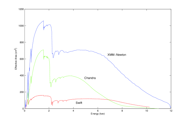
Figure 1: Effective area of the Swift XRT, Chandra-ACIS and XMM-Epic detectors

In practice, the input spectrum is a power-law continuum plus a gaussian $K\alpha$ iron line, taking into account the absorption by the galactic medium (wabs*(powerlaw+gaussian)). For this model, we have to input 6 initial parameters: (a) galactic column density, (b)power-law continuum power-law index, (c)continuum flux normalization factor, (d) gaussian line energy, (e) line width, and (f) normalization for the gaussian line. The galactic column density was set to a typical value $2\times 10^{20}\ {\rm cm^{-2}}$ (N. Brandt 2003, private communication). The continuum normalization is determined by the continuum flux given by the formula (1), making those two fluxes consistent over the instrument observing band (e.g. 0.2-10 keV). Because the simulated spectrum is seen in the observer frame, the Gaussian line energy is given by the equation $E_{l}=6.7\ {\rm keV}/(1+z)$. The line width is taken to be proportional to the line energy. Observationally, there is no consensus on how much the “typical” line width is. For the same burst GRB 991216, Piro (2000) obtained a line width of $\sigma>1$ keV, while Ballantyne et al. (2002) used a narrow line ($\sigma=0.01$ keV) to get a better fit. However, it is reasonable to assume it to be a broad line, because physically the photoionization of Fe-rich plasmas for an ionization parameter $\xi\sim 10^{3}$ is expected to result in an equilibrium rest-frame temperature of a few keV. In the simulations, we have used a fixed relation between the line energy and the line width, which for the most part is $\sigma_{l}=0.1\ E_{line}$ keV (except where we compared broad vs. narrow lines).The last parameter (f) is the equivalent width $EW$, which for the constant $EW$ models is set to be 1 keV, and in the varying $EW$ case it is given by the time dependence discussed above leading to a value $\sim 1$ keV at about one day.

(ii) Once we have the simulated spectrum, we follow the standard method of analyzing the spectrum using the XPSEC software package and determine to what degree the line is detectable, calculating the significance level (in standard deviations $\sigma$) for one specific detection according to the F-test.

(iii) We repeat the steps ((i) and (ii)) for at least 100 times, and check the repeatability of the detection rate of a line at a certain significance level.

In addition, we have also tested the degree to which instruments can differentiate a broad line from a narrow line, or distinguish between lines with different central energies, such as 6.4 and 6.7 keV. This is of interest as a diagnostic for the dynamics and thermal conditions in the emission region, which would provide a valuable tool in assessing models. The procedure used for these two tests are similar to those described above. The simulated spectra are obtained assuming the same input parameters as before. Each simulated spectrum is fitted with a power law and a fixed rest-frame line energy at either 6.4 keV or 6.7 keV, and we check the chi-square difference between the two fits, which indicates how the change of line energy affects the fit result. We repeated this fit and comparison procedure for each set of parameters 50 times, in order to reduce the statistical errors, and derive from this an average chi-square difference. Based on the chi-square difference, we find the corresponding probability, which is a function of the chi-square difference and the degrees of freedom (Chapter 15.6, Numerical Recipes in C++, Press et al. 2002). For example, a chi-square difference of 21 and 5 degrees of freedom corresponds to a probability 0.999, which is 3 $\sigma$. For the narrow line versus broad line test, we fixed as examples the line width to be 670 eV (broad line) and 200 eV (narrower line), respectively, in the rest frame, and follow a similar procedure as above for the line energy test.

Note that in our simulations we have used the chi-square statistics throughout, instead of likelihood statistics, which is valid and guaranteed by the large enough number of photons in each bin (at least 20 photons) and in total (usually thousand of photons collected during the whole integration time).

3 Simulation Results: Line Detection Significance

We have done simulations for several sets of GRB afterglow model parameters. The source-frame duration of the GRB is taken to be $T^{\prime}=20$ s or $T^{\prime}=40$ s. We show only the plots for $T^{\prime}=20$ s, the longer durations being used only for comparison. The initial isotropic-equivalent luminosity is usually taken to be $L_{X,0}=10^{50}\ {\rm ergs\ s^{-1}}$, consistent with the present ($z\lower 4.0pt\hbox{$\buildrel<\over{\sim}$}$ few) observations (Costa 1998). As an alternative, we also consider a higher than usual initial X-ray luminosity, $L_{X,0}=10^{51}$ erg s^-1, which might be typical of high redshift GRB, e.g. Schneider et al, 2002). (Note that we take an initial X-ray luminosity which is assumed to be about one order of magnitude below the corresponding prompt $\gamma$-ray luminosity). The source-frame equivalent width is typically taken as $EW^{\prime}=1.0$ or 0.5 keV (only the 1 keV results are shown). We consider the two generic line temporal behaviors discussed above, one in which the K$\alpha$ line has a a large $EW^{\prime}\sim 1{\rm keV}\sim$ constant from minutes after the trigger up to days, and another in which the $EW^{\prime}$ starts low, grows to $EW^{\prime}\sim 1$ keV on a timescale $\sim 1$ day, and drops rapidly afterwards (see discussion in §2). The integration time was taken to be 0.6 times the observing time, counted after the GRB trigger (i.e. for an observer time 1 day we take we take an integration time of 0.6 days ending at 1 day.

We took a grid of values in redshift $z$ and observer time $t$, and with the above parameters and the procedure outlined in the previous section we calculate for each pair of $z,t$ values the significance level of the detection with various instruments. For most of the calculations (unless stated otherwise) this procedure is repeated 300 times for each point, and the average chi-squared value is adopted, resulting in contour plots of the standard deviation $\sigma$ in the $z,t$ plane. E.g., regions in the plot with significance levels $\lower 4.0pt\hbox{$\buildrel>\over{\sim}$}3\sigma$ indicate that the detection is likely to be real.

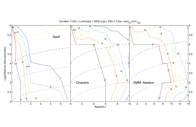
Figure 2: Fe K-$\alpha$ detection significance level contour plot for Swift (left), Chandra (middle) and XMM (right), assuming a source-frame GRB duration $T^{\prime}=20$ s and a constant $EW^{\prime}=1.0$ keV, initial X-ray luminosity $L_{X,0}=10^{50}\ {\rm ergs}\ {\rm s^{-1}}$ and integration time $t_{int}=0.6\ t_{obs}$. The dashed lines indicate contours of constant source-frame time.

Fig 2 shows the line detection significance levels attainable with Swift, Chandra and XMM for a burst of initial X-ray luminosity $L_{X,0}=10^{50}\ {\rm ergs}\ {\rm s^{-1}}$, source-frame equivalent width $EW^{\prime}=1.0$ keV (assumed constant), for a source-frame GRB prompt duration $T^{\prime}=20$ s. This shows that Swift can detect such iron lines with significance $\lower 4.0pt\hbox{$\buildrel>\over{\sim}$}4\sigma$ up to $z\lower 4.0pt\hbox{$\buildrel<\over{\sim}$}1.5$ for observer times $t\lower 4.0pt\hbox{$\buildrel<\over{\sim}$}10^{3}$ s, or up to $z\lower 4.0pt\hbox{$\buildrel<\over{\sim}$}1.2$ for observer times $t\lower 4.0pt\hbox{$\buildrel<\over{\sim}$}10^{4}$ s. to $z\lower 4.0pt\hbox{$\buildrel<\over{\sim}$}1$ for observer times up to a day. The bends in the significance level plots, e.g. at intermediate redshifts and times for Swift, are due to the minima in the effective area of the instrument at intermediate energies (figure 1). This is superposed on the expected overall tendency of a decreasing significance level with increasing time and redshift. For longer burst durations, e.g. $T^{\prime}$=40 s, the continuum flux level is correspondingly higher at the same time, and the lines are detectable to correspondingly higher redshifts or times. For a decreased equivalent width, e.g. $EW^{\prime}=$0.5 keV, Swift can detect such iron lines only in very nearby ($z\lesssim 0.3$) afterglows at a significance level of $\lower 4.0pt\hbox{$\buildrel>\over{\sim}$}4\sigma$, at observer times up to a day.

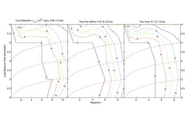
Figure 3: Bursts of higher initial luminosity $L_{X,0}=10^{51}$ ergs s^-1 observed by Swift. Shown is the ability to detect an Fe-$\alpha$ line (Left panel). Also shown is the ability to distinguish Fe 6.7 keV lines of different widths $\Delta E$=0.67 keV vs. $\Delta E$=0.2 keV (Middle panel), and to distinguish two lines of different central energies 6.7 keV (He-like Fe) vs. 7.2 keV (He-like Co) (Right panel). The contour levels give the significance for separating the two lines. In all cases, $EW^{\prime}=1.0$ keV, GRB duration $T^{\prime}=20$ s, and integration time $t_{int}=0.6\ t_{obs}$.

The same calculations for the same burst with the Chandra ACIS detector (Fig. 2, middle) and the XMM Epic detector (Fig 2, right) show a significantly greater depth of detection, as is to be expected from the larger effective areas. In all cases, the significance levels become lower as the observing time increases, as expected from the dimming, hence an earlier acquisition of the target as well as an early turn-on of the line improve the chances of detection. These plots also show features which are due to the detector characteristics. Roughly, one can say that bursts with the standard parameters used here would be detectable at better than $4\sigma$ confidence level with Chandra up to $z\lower 4.0pt\hbox{$\buildrel<\over{\sim}$}6-6.5$, and with XMM up to $z\lower 4.0pt\hbox{$\buildrel<\over{\sim}$}8.5-9$, at observer times $\lower 4.0pt\hbox{$\buildrel<\over{\sim}$}10^{5}$ s = 1 day. For later observer times, similar significance may be obtained for lower redshifts.

Fig 3 (left panel) shows the Swift line detection ability for a higher initial X-ray luminosity case, $L_{X,0}\sim 10^{51}\ {\rm erg\ s^{-1}}$, and constant $EW^{\prime}$ =1.0 keV. Such values may occur occasionally at moderate to low redshifts, and may also characterize bursts from very massive pop. III stars at large redshifts $z\lower 4.0pt\hbox{$\buildrel>\over{\sim}$}6$ (Schneider et al. 2002). For such higher initial fluxes, Swift may be able to detect lines at those high redshifts, while Chandra and XMM would do even better. Results for Swift in Fig. 3 (left panel) show that Fe lines would be detectable to better than $4\sigma$ up to $z\lower 4.0pt\hbox{$\buildrel<\over{\sim}$}8$ for observed times $t\lower 4.0pt\hbox{$\buildrel<\over{\sim}$}10^{5}$ s. (For $EW^{\prime}=0.5$ keV, not shown, this significance is achievable only to $z\lower 4.0pt\hbox{$\buildrel<\over{\sim}$}3.5$ and $t\lower 4.0pt\hbox{$\buildrel<\over{\sim}$}10^{4}$ s). There is a significant difference between the redshifts for, say, a $5\sigma$ line detection in the $L_{x,0}=10^{50}$ erg/s and for $L_{x,0}=10^{51}$ erg/s cases. For the lower luminosity case, this significance extends only up to $z\sim 1$, while for the higher luminosity the same significance level is reached up to $z\sim 7$. The difference is due mainly to two factors. First, the K-correction factor $(1+z)^{-1-a+b1}\sim(1+z)^{-1.4}$ (for the parameters used in the paper) compensates in part for the flux reduction as the luminosity distance increases with redshift. Second, there is a detector effective area difference between low and high redshift lines, which from Fig. 1 is seen to a factor $\sim 2$ increase in effective area for lines at $z\sim 7$ relative to those at $z\sim 1$.

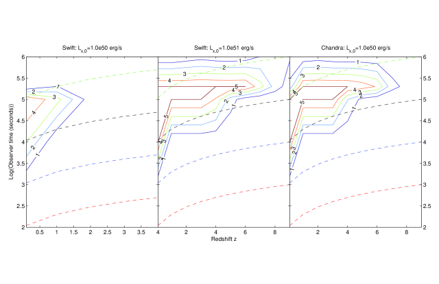
Figure 4: Variable equivalent width case, for a standard luminosity burst $L_{X,0}=10^{50}$ erg/s seen with Swift (left), a higher luminosity burst $L_{X,0}=10^{51}$ erg/s seen with Swift (middle), and a standard luminosity burst $L_{X,0}=10^{50}$ erg/s seen with Chandra (right). Shown are the line detection significance contours, in all cases the $EW$ peaks at 1 keV at one day in the rest frame (see text). Other parameters and symbols are the same as in Fig. 2

.

Fig 4 shows the line detectability by Swift in the case of a varying $EW$, using the $EW$ behavior with time calculated by Ballantyne & Ramirez-Ruiz, as discussed in §2. The most prominent characteristic on this plot is that the region where the detection confidence level is high lies, as expected, inside a strip corresponding to source times between $10^{4.5}$ and $10^{5.5}$ s. For the case of Swift and the standard initial luminosity $L_{X,0}=10^{50}\ {\rm ergs}\ {\rm s^{-1}}$ the $4\sigma$ level is achieved for $z\lower 4.0pt\hbox{$\buildrel<\over{\sim}$}0.7$ and observer times $t\sim 10^{4.5}-10^{5}$ s, while for the higher $L_{X,0}=10^{51}\ {\rm ergs}\ {\rm s^{-1}}$ case this is achieved at $z\lower 4.0pt\hbox{$\buildrel<\over{\sim}$}6$ and $10^{4.5}-10^{5.5}$ s (left and middle panels of Fig. 4). Most of the area on the plot outside this ridge shows a low significance, as expected, since in this case for initial observer time $\sim 10^{4}$ s, and also after $\sim 10^{5.5}$ s, the iron lines have a low $EW$ and are too weak to be detected. Comparing with the $EW$-constant case for the same parameters, the detectability of the varying $EW$ result near the peak is consistent with what is obtained in the constant $EW$ case. With Chandra, the same varying $EW$ case but with the standard initial luminosity $L_{X,0}=10^{50}\ {\rm ergs}\ {\rm s^{-1}}$ indicates that detection at the $4\sigma$ level can be achieved up to $z\lower 4.0pt\hbox{$\buildrel<\over{\sim}$}5.5$ at $t\sim 10^{4.5}-10^{5.5}$ s.

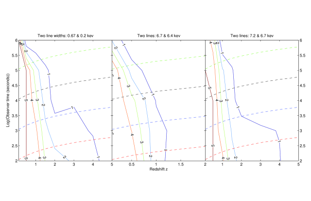
Figure 5: Swift ability to distinguish two Fe 6.7 keV lines of widths 0.67 keV vs. 0.2 keV (Left), or two Fe lines of the same width 0.67 keV and central energies 6.4 keV vs. 6.7 keV (Middle), or two lines of the same width but central energies 6.7 keV (He-like Fe) vs. 7.2 keV (He-like Co) (Right). The contour levels give the significance for separating the two lines, for standard bursts of initial X-ray luminosity $L_{X,0}=10^{50}$ ergs s^-1, $EW^{\prime}=1.0$ keV, GRB duration $T^{\prime}=20$ s, and integration time $t_{int}=0.6\ t_{obs}$.

Another useful calculation is to find the maximum redshifts and times for which various instruments can still distinguish a narrow from a broad line, or between different line energies, say between Fe 6.4 keV vs. 6.7 keV, or between corresponding Fe and Co K-$\alpha$ lines. For determining the significance level to which line differences can be measured, we follow the method discussed in §2. In principle, one might expect that when the line broadening decreases below the nominal energy resolution of a detector, one cannot differentiate between widths below this value. The resolution of the Chandra ACIS S3 instrument is $\sim 0.1$ keV, and that of the Swift XRT detector is $\sim 0.3$ keV. Thus with Chandra, for a line width of 0.67 keV, or 10% of the rest frame line energy, the observed line width for a GRB at $z\sim 6$ would be at the nominal energy resolution limit. However, even if this redshift is exceeded, or if the line is narrower, different width lines may still be distinguishable in a statistical way. The distinguishability of different line broadenings or line energies is affected by several additonal factors, such as the $EW$, the integration time, the degree to which the centroid of the lines can be characterized, etc.

Figure 6: Chandra ability to distinguish two Fe 6.7 keV lines of widths 0.67 keV vs. 0.2 keV (Left), or two Fe lines of the same width 0.67 keV and central energies 6.4 keV vs. 6.7 keV (Middle), or two lines of the same width but central energies 6.7 keV (He-like Fe) vs. 7.2 keV (He-like Co) (Right) . The contour levels give the significance for separating the two lines, for standard bursts of initial X-ray luminosity $L_{X,0}=10^{50}$ ergs s^-1, $EW^{\prime}=1.0$ keV, GRB duration $T^{\prime}=20$ s, and integration time $t_{int}=0.6\ t_{obs}$.

In practice, using XSPEC and the averaging of multiple tries described above, the maximum redshift to which lines of different broadenings can be differentiated is found to be somewhat larger than what is expected from the simple estimate above. In our simulations, we have taken a nominal “broad” line width of 0.67 keV (10% of the line energy) and a nominal ”narrow” line width of 0.2 keV, for the Fe K$\alpha$ 6.7 keV line. The results for Swift are shown in the left panel of Fig 5, while the results for Chandra are shown in the left panel of Fig 6 and those for XMM are shown in the left panel of Fig 7, for the standard luminosity burst case.

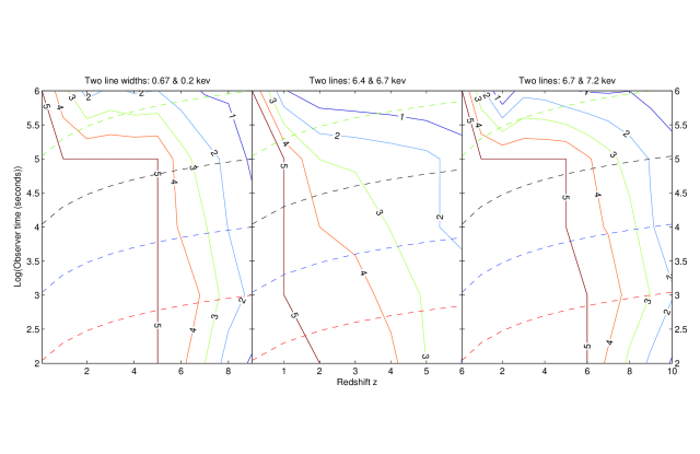
Figure 7: XMM-Newton ability to distinguish two Fe 6.7 keV lines of widths 0.67 keV vs. 0.2 keV (Left), or two Fe lines of the same width 0.67 keV and central energies 6.4 keV vs. 6.7 keV (Middle), or two lines of the same width but central energies 6.7 keV (He-like Fe) vs. 7.2 keV (He-like Co) (Right). The contour levels give the significance for separating the two lines, for standard bursts of initial X-ray luminosity $L_{X,0}=10^{50}$ ergs s^-1, $EW^{\prime}=1.0$ keV, GRB duration $T^{\prime}=20$ s, and integration time $t_{int}=0.6\ t_{obs}$.

For lines of different central energies, such as He-like Fe 6.7 keV K$\alpha$ and the lower ionization state Fe 6.4 keV line, the line energy difference is 0.3/(1+z) keV, and naively one expects a sensitivity to detecting different lines up to a redshift $z\sim 2$. The same factors, such as $EW$, integration time, etc, will affect the detectability. Using the statistical method described above, we have plotted for Swift in Fig 5, for Chandra in Fig 6, and for XMM-Newton in Fig 7 the significance contours for differentiating a 6.4 vs. a 6.7 keV line (middle panels).

We have also investigated the ability to distinguish between the He-like Fe 6.7 keV and the corresponding Co 7.2 keV or Ni 7.8 keV lines (which are all He-like) . We find that it is easier to distinguish Co or Ni He-like lines from the Fe 6.7 keV line than it is to distinguish between the Fe 6.7 and 6.4 keV lines, because the line energy differences are larger than that between Fe 6.4 and 6.7 keV lines. The significance contours for differentiating an Fe 6.7 keV from a Co 7.2 keV line are shown for Swift in Fig 5, for Chandra in Fig 6, and for XMM-Newton in Fig 7 (right panels, in all three), for a standard burst of initial X-ray luminosity $L_{x}=10^{50}$ erg/s, $EW^{\prime}=1.0$ keV, $T^{\prime}=20$ s. For bursts of higher initial luminosity $L_{X,0}=10^{51}$ erg/s, Swift’s ability to discriminate between Fe 6.7 keV and Co 7.2 keV lines is shown in the right panel of Fig 3.

We note that if lines of different widths or different energies are determined to be distinguishable with the above procedure, this implies that the lines are detectable at the 3 $\sigma$ or higher level. This is because in XSPEC, if a line is not detectable or is detectable at a smaller significance level, the possible parameter range does not make a significant difference in the fitting results. The converse, however, is not true, since there may be cases where a line is detectable at the 3 $\sigma$ level, while differences in the line energies or line widths cannot be distinguished at a comparable level of significance.

4 Discussion

We have quantitatively investigated the prospects for the detection of Fe group X-ray emission lines in gamma-ray burst afterglows, for various redshifts extending up to $z\sim 14$ and observing times extending up to 10 days after the trigger. We have used as a template for the X-ray continuum the spectral and temporal behavior inferred from afterglow observations, and have assumed Fe line rest-frame equivalent widths $EW^{\prime}\sim 1$ keV comparable to those reported in a number of GRB afterglows. These line and continuum models are purely phenomenological, without explicit reference to particular models. It is not known at present whether lines, if present, are formed soon after the outburst or only after periods of a day or so, as suggested by existing observations, since slewing time constraints in previous experiments prevented verification of the time of onset of the lines. Thus, we have tested for the line detectability at observer times starting at $t\sim 100$ s and up to days. We have assumed two simplified models for the equivalent width time behavior, motivated by generic analytical and numerical photoionization models. One of these assumes an equivalent width which does not change significantly with time, being a constant fraction of the photoionizing continuum. This model may be pertinent to so-called nearby models of line formation in the jet funnel or outer parts of the expanding star. The other assumes an equivalent width which grows in time up to a maximum value reached at about one day, and subsequently declines. This is motivated by so-called distant, or geometric models, e.g. where a shell of dense material is encountered at about a light day from the source. A similar behavior, however, may occur for some values of the parameters also in nearby models.

The results for simulated observations with the X-ray detectors in Swift (XRT), Chandra (ACIS S3) and XMM (Epic) are presented as contour plots of the significance level of line detection, expressed in standard deviations, for a Gaussian line of constant or varying equivalent width superposed on a power law continuum declining in time, as a function of redshift and observing time. As expected, the line detectability is sensitively dependent on the initial and subsequent continuum X-ray luminosity and on the equivalent width. Due to the K-correction effects whereby the spectral and temporal redshift-dependent changes partially cancel out, the sensitivity decrease in a given energy band with increasing redshift is more moderate than one would naively expect from the bolometric decay. Notice that this is dependent on the afterglow spectral and temporal indices entering in $F_{E}\propto E^{a}t^{b}$. For the nominal values adopted here, $a=-0.7$, $b=b1=-1.1$ (before the break), the K-correction is $(1+z)^{-1.4}$, but the specific values can differ substantially between bursts.

For an initial X-ray isotropic-equivalent luminosity $L_{X,0}=10^{50}$ erg/s, a constant source-frame equivalent width $EW^{\prime}=1.0$ keV and a prompt-phase source-frame duration $T^{\prime}=20$ s, Swift, Chandra, and XMM can detect lines with significance $\lower 4.0pt\hbox{$\buildrel>\over{\sim}$}4\sigma$ roughly out to $z\lower 4.0pt\hbox{$\buildrel<\over{\sim}$}1.5,\ 6,{\rm and}\ 8.5$ respectively (Fig 2), for times of order $t\lower 4.0pt\hbox{$\buildrel<\over{\sim}$}10^{3},~{}10^{5},~{}10^{5}$ s. For a similar initial luminosity but an equivalent width $EW^{\prime}=0.5$ keV, the corresponding redshifts drop substantially; e.g. Swift and Chandra could detect lines to $z\lower 4.0pt\hbox{$\buildrel<\over{\sim}$}0.3\ {\rm and}\ 2$, respectively, with the same confidence level as above for times of $t\lower 4.0pt\hbox{$\buildrel<\over{\sim}$}10^{3},~{}10^{5}$ s.

In a more detailed model, the equivalent width could vary in time, and in this case one would expect the line detectability to be maximal when the equivalent width reaches its peak value (See §2 for detailed model). Outside the peak range, the $EW$ is smaller and the detectablity drops rapidly. Our calculations for a standard luminosity burst of $L_{X,0}=10^{50}$ erg/s indicate that Swift could detect Fe lines up to $z\lower 4.0pt\hbox{$\buildrel<\over{\sim}$}0.7$ for times $t\lower 4.0pt\hbox{$\buildrel<\over{\sim}$}10^{4.5}-10^{5}$ seconds (Fig 4, left). For the same parameters, Chandra could detect Fe lines out to $z\lower 4.0pt\hbox{$\buildrel<\over{\sim}$}5.5$ for times of $\lower 4.0pt\hbox{$\buildrel<\over{\sim}$}10^{4.5}-10^{5}$ seconds (Fig 4, right). For more luminous afterglows of $L_{X,0}=10^{51}$ erg/s (which may be characteristic of pop. III bursts), Fe lines could be detected with Swift out to $z\lower 4.0pt\hbox{$\buildrel<\over{\sim}$}6$ with the same confidence level and observer time range as Chandra does for the standard (lower) luminosity case.

An interesting question is how far and how late can various instruments distinguish between lines of the same energy centroid but different widths, or between lines of similar widths but different energy centroids. The former is more difficult, especially at high redshifts or late times when the detection is marginal, and for this we investigated the distinguishability of nominal ”broad” lines with $\Delta E/E\sim$ 0.1 vs. ”narrow” lines with $\Delta E/E\sim$ 0.03, i.e. 0.6 keV vs. 0.2 keV widths for the Fe 6.7 keV lines. For investigating the sensibility to different line centroids, we assumed the same widths $\Delta E=0.67$ keV for lines of centroid energies 6.7 keV vs. 6.4 keV (He-like Fe vs. the lower ionization Fe line complex), as well as 6.7 keV (He-like Fe) vs. 7.2 keV (He-like Co). For a standard luminosity afterglow of $L_{X,0}=10^{50}$ erg/s and a constant equivalent width $EW^{\prime}=1.0$ keV, $T^{\prime}=20$ s, the figures (5), (6) and (7) show the ability to distinguish these different line cases with Swift, Chandra and XMM-Newton, respectively. One sees that for such standard luminosity bursts, Swift can differentiate an 0.67 keV line width from an 0.2 keV width out to $z\lower 4.0pt\hbox{$\buildrel<\over{\sim}$}1.2$ with confidence level of $\lower 4.0pt\hbox{$\buildrel<\over{\sim}$}4\sigma$ for times $t\lower 4.0pt\hbox{$\buildrel<\over{\sim}$}10^{3.5}$ s. It it can distinguish a 6.7 keV line from a 6.4 keV line out to $z\lower 4.0pt\hbox{$\buildrel<\over{\sim}$}0.2$ with confidence level $\sim 4\sigma$ at times $t\lower 4.0pt\hbox{$\buildrel<\over{\sim}$}10^{5}$ seconds; and a 6.7 keV line from a 7.2 keV line out to $z\sim 0.75$ with $\lower 4.0pt\hbox{$\buildrel<\over{\sim}$}4\sigma$ for times $t\lower 4.0pt\hbox{$\buildrel<\over{\sim}$}10^{5}$ s. As might be expected, a 7.2 keV line is easier to distinguish from a 6.7 keV than the latter is from a 6.4 keV line, since the energy difference is larger. Because Chandra and XMM have much larger effective areas, one expects that they can make such distinctions out to larger redshifts and longer times, as is verified from an inspection of fig 2 (middle and right panels). E.g. with Chandra, and $L_{X,0}=10^{50}$ erg/s, $EW^{\prime}=1.0$ keV, the same line width differences can be distinguished out to roughly $z\sim 1.5$ and $t\lower 4.0pt\hbox{$\buildrel<\over{\sim}$}10^{5}$ s with a confidence level $\sim 4\sigma$ (Fig 6, left), and energy differences of 6.4 vs. 6.7 keV out to $z\sim 1$ and $t\lower 4.0pt\hbox{$\buildrel<\over{\sim}$}10^{4.5}$ s (Fig 6, middle); while energy difference of 6.7 vs. 7.2 keV can be distinguished out to $z\sim 1.8$ and $t\lower 4.0pt\hbox{$\buildrel<\over{\sim}$}10^{4.5}$ s with $\sim 4\sigma$( Fig 6, right). For XMM, the corresponding redshifts are of order is $z\lower 4.0pt\hbox{$\buildrel<\over{\sim}$}5.5,\ 1.5,\ 6$ with a confidence level of $\lower 4.0pt\hbox{$\buildrel<\over{\sim}$}4\sigma$ for times of order $10^{5}$ s (Fig 7).

For larger initial isotropic-equivalent X-ray luminosities, e.g. $L_{X,0}=10^{51}$ erg/s corresponding to an extreme low-resdhift case or a nominal high-redshift pop. III case, Swift (and of course Chandra and XMM) can detect lines out to much higher redshifts compared to the standard case of $L_{X,0}=10^{50}$ erg/s. This is shown in Fig 3, where for a constant $EW^{\prime}=1.0$ keV and $T^{\prime}=20$ s the maximum $4\sigma$ redshifts at $t\sim 10^{5}$ s are $z\sim 8$, $6$, and $5.5$ for the detection of a 6.7 keV line, for distinguishing two line widths of 0.67 vs. 0.2 keV, and for distinguishing two lines of 6.7 vs. 7.2 keV (left, middle and right panels, respectively).

In conclusion, if X-ray lines are present in GRB, Chandra and XMM, with their slower slew response times, should be able to detect them at observer times $\lower 4.0pt\hbox{$\buildrel>\over{\sim}$}0.5$ days ($0.5/(1+z)$ days in the source frame) out to very high redshifts $z\sim 7-10$, in the range where the universe started to reionize, for burst properties similar to those inferred in $z\sim 1-3$ objects. If XMM and Chandra do not detect new lines at a higher significance level than previously reported (noting that line evidence is considered currently for 9 out of 21 bursts, e.g. Sako et al. 2004), one might conclude that the conditions assumed here do not apply to some or all of the bursts; or the $EW$ are smaller (e.g. as in the variable $EW$ case, see Fig 4); or the luminosity is smaller; or the lines do not appear early on, when the flux is high, etc. If on the other hand lines are detected, XMM and Chandra should also be able to distinguish details such as line widths or central energies out to redshifts where the first galaxies formed, $z\sim 6$. Swift, with its fast slew time, should be able to detect lines at much earlier times, if present, starting at $t\sim 10^{2}-10^{3}$ s, and out to redshifts $z\sim 1.5$, or to higher redshifst for the more luminous bursts. In the latter case, it would also be able to answer questions about line broadening, ionization stage or line physics out to $z\lower 4.0pt\hbox{$\buildrel<\over{\sim}$}0.8$ and times up to a day.

Thus Swift, in conjunction with larger spacecraft such as Chandra and XMM, should be able to answer important questions about burst properties as a function of the age of the universe, such as whether X-ray lines occur in them, at what times in the source frame they form, and out to what redshifts, as well as details of the physical conditions in the burst.

References

- (1) Amati, L., et al. 2000, Science, 290, 953
- (2) Antonelli, A., et al. 2000, ApJ, 545, L39
- (3) Ballantyne, D.R., et al. 2002, A&A, 389, L74
- (4) Böttcher M., & Fryer, C.L. 2001 ApJ, 547, 338
- (5) Costa, E. 1999, A&AS, 138, 425
- (6) Ghisellini, G., et al. 1999, A&AS, 138, 545
- (7) Ghisellini, G., et al. 1999, ApJ, 517, 168
- (8) Ghisellini, G., et al. 2002, A&A, 389, L33
- (9) Kallman, T., Mészáros , P. & Rees, M.J. 2003, ApJ, 593, 946
- (10) Lazzati, D., Campana, S., & Ghisellini, G. 1999, MNRAS, 304, L31
- (11) Lazzati, D., Campana, S., & Ghisellini, G. 1999, A&AS, 138, 547
- (12) Lazzati, D., Ramirez-Ruiz, E., & Rees, M.J. 2002, ApJ, 572, L57
- (13) Mészáros , P. & Rees, M.J. 2001, ApJ, 556, L37
- (14) Mészáros , P. & Rees, M.J. 2003, ApJ, 591, L91
- (15) Rees, M.J. & Mészáros , P. 2000, ApJ, 545, 73
- (16) Reeves, J. et al. 2002, Nature, 416, 512
- (17) O’Brian, P.T., et al. 2003, astro-ph/0312602
- (18) Piro, L., et al. 1999, ApJ, 514, L73
- (19) Piro, L., et al. 2000, Science, 290, 955
- (20) Press, W.H., Teukolsky, S.A., Vetterling, W.T., & Flannery, B.P., 2002, Numerical Recipes in C++, Cambridge University Press
- (21) Sako, M., Harrison, F. & Rutledge, R.E., 2004, astro-ph/0406210
- (22) Schneider, R., Guetta,D., & Ferrara, A. 2002, MNRAS, 334, 173
- (23) Watson, D., et al. 2002, A&A, 393, L1
- (24) Watson, D., et al. 2003, ApJ, 595, L29
- (25) Weth, C., Mészáros , P., Kallman, T., & Rees, M.J. 2000, ApJ, 534, 581
- (26) Yoshida, A., et al. 1999, A&ASS, 138, 433