Towards a More Standardized Candle Using GRB Energetics and Spectra

Abstract

The use of $\gamma$-ray bursts (GRBs) energetics for cosmography has long been advanced as a means to probe out to high redshifts, to the epoch of deceleration. However, though relatively immune to systematic biases from dust extinction, the prompt energy release in GRBs, even when corrected for jetting geometry, is far from being a standard candle. In this work, we explore the cosmographic potential of a GRB standard candle based on the newly-discovered relation by Ghirlanda et al. between the apparent geometry-corrected energies ($E_{\gamma}$) and the peak in the rest frame prompt burst spectrum ($E_{p}$). We present an explicit, self-consistent formalism for correcting GRB energies with a thorough accounting for observational uncertainties. In contrast to other work, we demonstrate that the current sample of 19 GRBs is not yet cosmographically competitive to results from Type Ia supernovae, large-scale structure, and the microwave background. Although the $E_{p}$–$E_{\gamma}$ relation is a highly significant correlation across a range of cosmologies [$0\leq\Omega_{M},\ \Omega_{\Lambda}\leq 2$], the goodness of fit of the data to a power law ($E_{p}\propto E_{\gamma}^{\eta}$), depends strongly on input assumptions. The most important of these assumptions concern the unknown density (and density profile) of the circumburst medium, the efficiency of converting explosion energy to $\gamma$–rays, data selection choices for individual bursts (some of which were not included in similar work), and assumptions in the error analysis. Independent of assumptions, with very few low-$z$ bursts, the current sample is most sensitive to $\Omega_{M}$ but essentially insensitive to $\Omega_{\Lambda}$ (let alone the dark energy equation of state $w$). The proper use of the relation clearly brings GRBs an impressive step closer toward a standardizable candle, but until the physical origin of the $E_{p}$–$E_{\gamma}$ relation is understood, calibrated with a training set of low redshift (e.g., cosmology independent) bursts, and the major potential systematic uncertainties and selection effects are addressed, we urge caution concerning claims of the utility of GRBs for cosmography.

1 Introduction

As ultra-luminous explosions from the death of massive stars, gamma-ray bursts (GRBs) can, in principle, occur and be detected from redshifts at the epoch of reionization, serving as unique probes of the gas and metal-enrichment history in the early universe (e.g., Loeb & Barkana, 2001; Mészáros & Rees, 2003; Inoue, 2004). At such redshifts beyond $z\sim 7$, the dynamics of the universal expansion is not yet dominated by the cosmological constant $\Lambda$, so the construction of an early-universe Hubble diagram using GRBs would complement cosmography results found in the $\Lambda$-dominated regime at lower redshifts. Since $\gamma$-rays penetrate dust, a standard candle derived from GRB energetics could avoid potential systematic errors inherent in supernovae (SNe) due to uncertainties in dust extinction. Cosmological $k$-corrections for GRBs (Bloom et al., 2001b) are, in principle, more tractable than traditional optical $K$-corrections for SNe; where GRB spectra are devoid of emission/absorption features at $\gamma$-ray wavelengths, SNe spectra — due to the variety of filter bands used and uncertainty in the intrinsic spectral shape — are generally considered to contribute a redshift-dependent systematic error to SNe Ia magnitudes (Wang & Garnavich, 2001). Still, both samples necessarily contend with unknown evolution of the standard candle; but, owing to very different physics in the emission mechanisms, any such evolution would unlikely be the same for GRBs and SNe Ia.

Early attempts to meaningfully constrain cosmological parameters using GRB energetics were stymied (e.g., Dermer, 1992; Rutledge et al., 1995; Cohen & Piran, 1997) by what is now known (Bloom et al., 2001b; Schmidt, 2001) as a wide distribution — more than 3 orders-of-magnitude — in the intrinsic isotropic-equivalent energies ($E_{\rm iso}$) and luminosities of GRBs. The realization that GRBs are a jetted phenomena (Harrison et al., 1999; Stanek et al., 1999) led to the discovery that the geometry-corrected prompt energy release ($E_{\gamma}$) in GRBs appears nearly constant ($\sim$10⁵¹ erg $\equiv 1$ foe; Frail et al., 2001; Piran et al., 2001). This, along with the possibility of inferring GRB redshifts from the $\gamma$-ray properties alone (e.g., Reichart et al., 2001; Norris, 2002), renewed enthusiasm for the cosmographic utility of GRBs (Schaefer, 2003; Takahashi et al., 2003). Frail et al. (2001) had noted this apparent constancy for what was then the current sample of 17 GRBs with known redshifts. Bloom et al. (2003b), with an expanded sample of 29 GRBs with known $z$, later argued that even geometry-corrected energetics were not sufficient for cosmography on both conceptual and empirical grounds. First, while the physical motivation for a standard energy release is plausible, the geometry correction of $E_{\rm iso}$ is highly model dependent, requiring an inference of the nature of the circumburst environment and assumptions about the structure of the jet. This problem persists even with new energy corrections detailed herein. Second, the cosmographic utility of $E_{\gamma}$ was limited by the presence of several low energy and high energy outliers, comprising upwards of 20% of the sample, spanning three orders of magnitude (GRB 980425 aside). Bloom et al. (2003b) argued that without an energy-independent discriminant (such as properties of the afterglow) such outliers could not be excluded (or re-calibrated) a priori when constructing a GRB Hubble Diagram. A regularization of $E_{\gamma}$ would require a universal relation between $E_{\gamma}$ and other observables.

The recent discovery of a connection between $E_{\gamma}$ and the peak energy ($E_{p}$) in the rest-frame prompt burst spectrum (Ghirlanda et al., 2004a) is apparently such a universal relation spanning the hardest, brightest bursts to the softest, faintest X-ray Flashes (XRFs; Heise et al. 2001). In this paper, we demonstrate that this $E_{\gamma}$–$E_{p}$ (“Ghirlanda”) relation can serve as an approximate empirical correction to GRB energies, advancing GRB energetics towards a more standardized candle. In presenting the formalism for correcting GRB energetics, we draw a strong analogy between our corrections and the empirical light-curve shape corrections (based upon the peak brightness–decline rate correlation) used to standardize the peak magnitudes of Type Ia SNe (Phillips, 1993; Hamuy et al., 1995, 1996; Riess et al., 1995, 1996; Perlmutter et al., 1997; Tonry et al., 2003). In § 2 we confirm the $E_{p}$–$E_{\gamma}$ relation and show that although the goodness of fit to the simple power-law relation is highly sensitive to input assumptions, the correlation itself is still highly significant over a variety of plausible cosmologies. In § 3 we introduce a new formalism, with an explicit accounting for observational uncertainties, for correcting GRB energies. In § 4 we discuss similar work from Dai et al. (2004) and Ghirlanda et al. (2004c), noting critical differences in our respective methodologies and datasets. We then attempt to lay the groundwork for identifying relevant systematic errors and selection effects in § 5 and end with a discussion of the future prospects of an even more standardized GRB energy. Unless otherwise noted, we assume a standard cosmology of ($\Omega_{M}$, $\Omega_{\Lambda}$, $h=H_{0}/100$km s^-1 Mpc^-1) $=$ ($0.3,0.7,0.7$).

2 GRB Energetics and the $E_{p}$–$E_{\gamma}$ Relation Revisited

We compute the geometry-corrected prompt energy release in gamma-rays ($E_{\gamma}$) following Bloom et al. (2003b) and the associated uncertainties with a slightly improved formalism in § 2.1. All energies are computed using the “top hat” model prescription for the jet: the energy per steradian in the jet is assumed to be uniform inside some half-angle $\theta_{\rm jet}$ and zero outside (Rhoads, 1997; Sari et al., 1999). Following Frail et al. (2001), the total beaming corrected gamma-ray energy can be written as

$$E_{\gamma}=E_{\rm iso}f_{b}=\frac{4\pi S_{\gamma}\,k\,Dl_{\rm th}^{2}}{1+z}[1-\cos(\theta_{\rm jet})],$$ (1)

where $f_{b}=1-\cos(\theta_{\rm jet})$ is the beaming fraction, $z$ is the observed redshift, $Dl_{\rm th}$ is the theoretical luminosity distance for a given cosmology, $S_{\gamma}$ is the $\gamma$-ray fluence in the observed bandpass, and $k$ is the “cosmological $k$-correction” (Bloom et al., 2001b), a correction factor of order unity which blueshifts the observed redshifted GRB spectrum back into some “bolometric” cosmological rest-frame bandpass which we take as [20,2000] keV (Bloom et al., 2003b). See § 5.1 for a justification of this choice of bandpass. Following Sari et al. (1999), in the case of a homogeneous circumburst medium (“ISM”),

$$\theta_{\rm jet} = 0.101{\ \rm rad}\left(\frac{t_{\rm jet}}{1\ {\rm day}}\right)^{3/8}\left(\frac{\xi}{0.2}\right)^{1/8}\left(\frac{n}{10\ {\rm cm}^{-3}}\right)^{1/8}$$ (2)

$$\times\left(\frac{1+z}{2}\right)^{-3/8}\left(\frac{E_{\rm iso}}{10^{53}\ {\rm erg}}\right)^{-1/8},$$

where $z$ is the redshift, $t_{\rm jet}$ is the afterglow jet break time, $n$ is the density of the ambient medium (ISM), $E_{\rm iso}$ is defined via eq. 1, and $\xi$ is the efficiency for converting the explosion energy to $\gamma$-rays. For simplicity in the later formalism, we write eq. 2 as $\theta_{\rm jet}=B\ t_{\rm jet}^{3/8}\xi^{1/8}{n}^{1/8}(1+z)^{-3/8}E_{\rm iso}^{-1/8}$ defining the constant $B=0.101(1\,{\rm day})^{-3/8}(0.2)^{-1/8}(10$ cm${}^{-3})^{-1/8}(2)^{3/8}(10^{53}$ erg$)^{1/8}=5.08\times 10^{5}$ erg^1/8 cm^3/8 day^-3/8 which absorbs the relevant units. See § 5.4 for a discussion of how the analysis changes for a circumburst medium that is not homogeneous, for example, a wind profile from a massive star (Chevalier & Li, 1999, 2000).

2.1 Error Analysis

We estimate the uncertainty in $E_{\gamma}$ under the assumption of no covariance between the measurement of the observables $S_{\gamma}$, $k$, $t_{\rm jet}$, and $n$, and the inference of $\theta_{\rm jet}$. We assume the error in the determination of the redshift $z$ is negligible. We also assume priors on the Hubble constant ($h=0.7$) and $\gamma$–ray efficiency ($\xi=0.2$), each with no error. Under these assumptions, the fractional uncertainty in $E_{\gamma}$ is given by

$$\left(\frac{\sigma_{E_{\gamma}}}{E_{\gamma}}\right)^{2} = \left(1-\sqrt{C_{\theta_{\rm jet}}}\right)^{2}\left[\left(\frac{\sigma_{S_{\gamma}}}{S_{\gamma}}\right)^{2}\ +\ \left(\frac{\sigma_{k}}{k}\right)^{2}\right]\$$

$$\ +\ C_{\theta_{\rm jet}}\left[9\left(\frac{\sigma_{t_{\rm jet}}}{t_{\rm jet}}\right)^{2}\ +\left(\frac{\sigma_{n}}{n}\right)^{2}\right]\$$

where $C_{\theta_{\rm jet}}$ is defined in eq. 5 of Bloom et al. (2003b). The above expression is slightly modified from eq. 4 of Bloom et al. (2003b) which also assumed no covariance, but in contrast, employed the approximation of ignoring the implicit $E_{\rm iso}$ dependence inside of $f_{b}$. This changes the multiplicative factor for the terms on the first line of eq. LABEL:eq:E_gamma_err from the old term $(1+C_{\theta_{\rm jet}})$ to the new term $\left(1-\sqrt{C_{\theta_{\rm jet}}}\right)^{2}$, indicating that eq. 4 of Bloom et al. (2003b) was, at worst, conservatively overestimating the error by about 25% for a typical burst.

While the above expression makes fewer assumptions than previous work, the assumption of no covariance (also discussed in Bloom et al. 2003b) still requires justification, which we defer to § 5.2. However, using the triangle inequality, we can place a firm upper limit on $\sigma_{E_{\gamma}}$ even assuming maximal covariance.

$$\left(\frac{\sigma_{E_{\gamma}}}{E_{\gamma}}\right) \leq \left(1-\sqrt{C_{\theta_{\rm jet}}}\right)\left[\left(\frac{\sigma_{S_{\gamma}}}{S_{\gamma}}\right)\ +\ \left(\frac{\sigma_{k}}{k}\right)\right]\$$ (4)

$$\ +\ \sqrt{C_{\theta_{\rm jet}}}\left[3\left(\frac{\sigma_{t_{\rm jet}}}{t_{\rm jet}}\right)\ +\ \left(\frac{\sigma_{n}}{n}\right)\right]$$

Evaluating this expression for a typical burst tells us that even maximal covariance (we argue it is nowhere near maximal in § 5.2) would mean we are underestimating the errors by at most a factor of $\lesssim 2$. As such, we believe the assumption of no covariance is a reasonable starting point, although, in the extreme case, a factor of two increase in the error bars would significantly affect the results.

2.2 Dataset Compilation

Computing $E_{\gamma}$, $\sigma_{E_{\gamma}}$, and constructing the Ghirlanda relation requires a compilation of all available data. The observables of interest include $z$, $S_{\gamma}$, $t_{\rm jet}$, $n$, and $\xi$, as defined in § 2. Also needed are the observed peak energy $E^{\rm obs}_{p}$ [$E_{p}=E^{\rm obs}_{p}(1+z)$], as well as the low energy and high energy spectral slopes $\alpha$ and $\beta$ of the Band function, respectively (Band et al., 1993). Ideally, high-energy measurements would be derived from a single satellite and inferences of afterglow parameters would be construed from consistent modeling with homogeneously-acquired data. In practice, however, we must compile a heterogeneous dataset with varying degrees of accuracy on parameters derived from different models and different instrumentation.

Still, in the interest of obtaining from the literature the highest quality and most homogeneous dataset possible, we abide by several guidelines. First, we preferentially choose $E^{\rm obs}_{p}$ measurements with reported error bars that have accompanying reports of $\alpha$ and $\beta$ with errors. Second, we use input fluence measurements with reported errors with priority over fluence measurements in wider bandpasses. Third, we choose the best sampled afterglow light curve with the smallest errors on the best fit value of $t_{\rm jet}$, preferring those estimations that use the earliest available afterglow data before the break. Measurements reported in published papers are assumed to supersede those given in GCN or IAU Circulars. Notes on the data selection for individual bursts are given in Appendix A.

Often, measurements on some non-critical input parameters to the energetics are not available (we of course exclude bursts from our analysis where no redshift, fluence, or jet-break time is known). For these, we choose a single value for every burst with an associated “measurement error”. In the absence of reported values of $\alpha$ or $\beta$ (there are no cases of both missing in our sample), we set $\alpha=-1$ and $\beta=-2.3$ as described in Appendix A. Following Frail et al. (2001), we also assume $\xi=0.2$ (20%) for all bursts (see § 5.6 for a critique of this assumption). Following Bloom et al. (2003b), we assume $n=10\pm 5$ cm^-3 (the 50% error assumption is new to this work) in the absence of constraints from broadband afterglow modeling (see § 5.5 for a discussion of this choice). We note, however, that the analysis is very sensitive to the assumptions for the circumburst density (and to a lesser extent, the $\gamma$–ray efficiency), as we show in sections § 2.4, § 2.5. In the absence of reported errors, we assume errors of 10% for $S_{\gamma}$ and 20% for $E^{\rm obs}_{p}$. These errors are reflective of those for bursts with reported errors (see Table Towards a More Standardized Candle Using GRB Energetics and Spectra). Errors on $t_{\rm jet}$ are available for all bursts in the set we use (although see Appendix A). All errors on the cosmological $k$-correction are computed via the formalism in Bloom et al. (2001b). These implicitly depend on the low energy slope $\alpha$, the high energy slope $\beta$, and the break energy $E^{\rm obs}_{o}=E^{\rm obs}_{p}(2+\alpha)$, of the Band Function (Band et al., 1993), and we assume 20% errors on these parameters when they are not reported – as these are also typical of reported errors. When asymmetric fluence or peak energy errors are reported in the literature (e.g., HETE II bursts; Sakamoto et al. 2004), we assume $\sigma_{S_{\gamma}}=\sqrt{\sigma_{S_{\gamma}}^{+}\sigma_{S_{\gamma}}^{-}}$, and the $\sigma_{E^{\rm obs}_{p}}=\sqrt{\sigma_{E^{\rm obs}_{p}}^{+}\sigma_{E^{\rm obs}_{p}}^{-}}$ (i.e., the geometric mean). This assumption has little effect on the overall analysis. Finally, we assume $h=0.7$ with no error to calculate the energetics.

The most current input data and reported errors are listed in Table Towards a More Standardized Candle Using GRB Energetics and Spectra. Again, see Appendix A concerning data selection for individual bursts. Since the Bloom et al. (2003b) energetics compilation, spectroscopic redshifts have been determined for 10 additional bursts: XRF 020903, GRB 030226, GRB 030323, GRB 030328, GRB 030329, XRF 030429, GRB 031203, XRF 040701, GRB 040924, and GRB 041006 for a total of 39 bursts with $z$, along with at least 4 upper limits: XRF 020427, GRB 030324, GRB 030528, and XRF 030723. Of these 14 bursts, 10 have measurements or constraints on $t_{\rm jet}$, along with 7 bursts where constraints have been added or updated from the Bloom et al. (2003b) sample. We use this updated list of GRB observables as inputs to the energetics calculations which follow. The $E_{\gamma}$ values (with errors) of these new bursts, and updates to the previous compilation are given in Table 2 for the standard cosmology.

2.3 Refitting the $E_{p}$-$E_{\gamma}$ relation

Limited to only those 23 bursts with redshifts and observed jet break times without upper or lower limits (hereafter, “Set E”), the median value of $\log(E_{\gamma}{\rm[erg]})$ is 50.90 ($\sim$ 1 foe) with an RMS scatter of 0.55 dex. Under our assumptions, the average fractional error on $E_{\gamma}$ for these bursts is $\sim 26\%$. Including 10 more bursts with upper or lower limits taken at face value does not significantly affect the median, yielding 50.91 ($\sim$ 1 foe), with an RMS of 0.55 dex. It should be noted that the RMS scatter actually is an overestimate of the true 1-$\sigma$ error on the median since the distribution is only approximately gaussian with a broad tail extending to low energies: as recognized by a number of authors, the low redshift burst GRB 030329 ($z=0.1685$), as well as GRB 990712, GRB 021211, and XRF 030429 all appear to be under-energetic by around 1 order of magnitude. Moreover the low redshift GRB 031203 ($z=0.1055$) along with XRFs 030723 ($z<2.1$) and 020903 ($z=0.251$) also appear under-luminous by at least $2$–$3$ orders-of-magnitude — even assuming an isotropic explosion — as the geometry correction is not known for these bursts.

Ghirlanda et al. (2004a) recognized that these under-luminous bursts appeared systematically softer in the prompt burst spectrum than bursts of apparent higher $E_{\gamma}$. Expanding upon the much discussed correlation (Amati et al., 2002) between the isotropic-equivalent energy $E_{\rm iso}$ and the restframe peak energy in the GRB spectrum ($E_{p}$), the authors discovered a remarkably strong correlation between $E_{\gamma}$ and $E_{p}$, which can be represented as a power-law:

$$E_{p}=\kappa\left(\frac{E_{\gamma}}{E^{*}}\right)^{\eta}$$ (5)

The scaling $E^{*}$ is a constant which we choose in order to minimize the covariance between $\eta$ and $\kappa$ when fitting for this two-parameter relation, simplifying future error analyses. This choice of $E^{*}$ does not affect the values of the best fit slope $\eta$ (or the goodness of fit) and the parameter $\kappa$ simply scales as $(E^{*})^{\eta}$.

Using an updated set including 19 bursts with redshifts, $E_{p}=E^{\rm obs}_{p}(1+z)$, and reported $t_{\rm jet}$ measurements without upper/lower limits (hereafter “Set A”), we confirm the strong correlation in the standard cosmology for the set of assumptions detailed in § 2, finding the best fit values of $\eta=$ 0.669 $\pm$ 0.034, $\kappa=$ 252 $\pm$ 11 keV ($E^{*}=4.14\times 10^{50}$ erg), with a Spearman $\rho$ correlation coefficient of 0.86 (null hypothesis probability of $2.9\times 10^{-6}$).

The relation for a standard cosmology is shown in Figure 1, with inset panel indicating the cosmology dependence, which is discussed in detail in § 3.3. Although the correlation is clearly significant, we find a reduced $\chi^{2}_{\nu}\equiv\chi^{2}/$dof = 3.71 (for 17 degrees of freedom; dof), suggesting that a single power-law does not adequately accommodate the data, given the assumptions and dataset compilation: we will address the dependence of $\chi^{2}/$dof on various assumptions in detail in § 2.4, § 2.5.

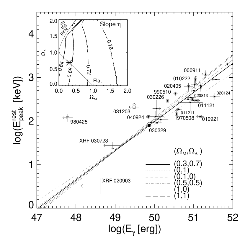
Figure 1: The (weak) cosmological dependence of the $E_{p}$–$E_{\gamma}$ relation. The best fit power-law relation for a representative set of cosmologies are shown as a series of lines. Only the derived $E_{\gamma}$ values in standard cosmology of ($\Omega_{M},\Omega_{\Lambda},h$)=($0.3,0.7,0.7$) are shown for clarity with upper/lower limits indicated with arrows. Set A is comprised of those bursts with no upper/lower limits (small filled squares), with a goodness of fit $\chi^{2}/$dof$=3.71$ (17 dof). Data are calculated for a bolometric rest frame bandpass of $[20,2000]$ keV, assuming a $\gamma$-ray production efficiency of $\xi=0.2$, and an external homogeneous ISM density of $n=10\pm 5$ cm^-3 when there are no reliable constraints from broadband afterglow modeling. Notable outliers under these assumptions are indicated with a large square surrounding the data points (small filled squares). GRBs 980425 and 031203 are major outliers regardless of their geometry correction or external density. The only outliers for which density is constrained are GRBs 970508 and 990510. As such, all other nominal outliers can be made consistent with the relation simply by changing the density (or increasing the error on the density), as discussed in § 2.5. With the current data, and our assumptions, XRFs 020903 and 030723 are consistent with the relation. Note GRB 030329, a large outlier in $E_{\gamma}$ (large filled black square), falls directly on the relation. The best fit value of the slope ($\eta$) is shown inset as a contour plot over the cosmological parameters ($\Omega_{M}$, $\Omega_{\Lambda}$). Over a wide range of cosmologies [$0\leq\Omega_{M}$, $\Omega_{\Lambda},\leq 2$], $\eta$ falls in a narrow range from $\sim 0.6$–$0.8$, with typical errors $\sim 0.03$–$0.5$ ($5$–$6\%$). Note that the data for a standard cosmology with best fit $\eta=$ 0.67 $\pm$ 0.03, (indicated by the asterisk in the inset contour plot, and the thick black best fit line in the outer plot), essentially brackets the fits across all cosmologies in the range [$0\leq\Omega_{M}$, $\Omega_{\Lambda}\leq 1$], $\eta\in[0.64,0.70]$, excepting only the extreme cosmologies with $\Omega_{M}\sim 0$ and $\Omega_{\Lambda}\sim 1$ or $\Omega_{M}\sim 1$. Thus, for a wide range of reasonable cosmologies, (not to mention $k$-correction bandpasses and external densities) the slope of the relation is $\sim 2/3$.

Despite the poor fit, Ghirlanda et al. (2004a) correctly noted that this power-law fit is better than the fit to the $E_{p}$–$E_{\rm iso}$ “Amati” relation $E_{p}=A\left(E_{\rm iso}/E^{\prime}\right)^{m}$ ($E^{\prime}=10^{52}$ erg). Indeed, for the subset of 29 bursts with measurements of redshift $z$, and $E_{p}$ without upper/lower limits (excluding GRB 980425), we find best fit $m=0.496\pm 0.037$, $A=90\pm 8$ keV and a Spearman $\rho$ correlation coefficient of $\rho=0.88$, with a null hypothesis probability of no correlation of $4.9\times 10^{-10}$. As originally recognized by Amati et al. (2002), the correlation is clearly significant. However the goodness of fit found here: $\chi^{2}_{\nu}\sim 9.48$ (27 dof), is clearly poorer than for the new Ghirlanda relation, and cannot easily be improved by changing input assumptions. Recent work (Nakar & Piran, 2004), indicates that a significant fraction of GRBs without known redshifts cannot fall on the Amati relation, which — due to selection effects — may be better understood as a demarcation of an upper limit (where burst energies can be no greater than their isotropic equivalents). This implies that any intrinsic spectra-Energy connection is more closely related to the Ghirlanda relation than the Amati relation; this is not surprising given the more physically motivated, beaming-corrected energy, rather than the poor approximation of energy inferred for a spherical explosion. However, see Band & Preece (2005) for a similar analysis of the Ghirlanda relation which raises the possibility that the relation itself could arise due to selection effects — mostly concerning the measurement of $t_{\rm jet}$, $E^{\rm obs}_{p}$, and $z$.

2.4 Comparison with Other Work

The $E_{p}$–$E_{\gamma}$ relation has been fit in several other works (Ghirlanda et al., 2004a, c; Dai et al., 2004) using different data sets and a range of input assumptions different from those assumed herein. We focus on comparing our results with the sample of Ghirlanda et al. (2004a) and Ghirlanda et al. (2004c): 15 bursts, hereafter “Set G”, which uses a more complete sample than that of Dai et al. (2004): 12 bursts, hereafter “Set D”. In contrast, our Set A contains 19 bursts (see our Table Towards a More Standardized Candle Using GRB Energetics and Spectra). The bursts belonging to each of these samples are noted in the leftmost column of our Table 2. For clarification, the Set name A, G, or D simply refers to the names of the bursts in the sample, not to the assumptions used by various groups or the individual references chosen for the data for a given burst, differences which are detailed in Appendix B. In referring below to the Ghirlanda et al. data, we refer to the overlapping subset of our data (Table Towards a More Standardized Candle Using GRB Energetics and Spectra) as G, and refer to the Ghirlanda et al. (2004a) data itself (their Tables 1-4), as G^∗, which uses their data selection and assumptions, and likewise for D (our Table Towards a More Standardized Candle Using GRB Energetics and Spectra) and D^∗ (Table 1 of Dai et al. 2004).

The parameterization of the $E_{p}$–$E_{\gamma}$ relation and the reported errors on the slope that we find; $\eta=0.669\pm 0.034$, $\chi^{2}_{\nu}$ =3.71 (17 dof), are consistent with those given in Ghirlanda et al. (2004a) and Ghirlanda et al. (2004c); $\eta=0.706\pm 0.047$, $\eta^{-1}=1.416\pm 0.09$, respectively. Both fits are performed in the standard ($\Omega_{M}$, $\Omega_{\Lambda}$, $h$) = (0.3, 0.7, 0.7), cosmology, but differ somewhat owing to the slightly larger sample used here to construct the fit (19 vs. 15 bursts), data selection differences for the bursts common to both samples (again, see Appendix A), differing assumptions for the density and its fractional error, as well as the different energy bandpass used for $E_{\gamma}$. We compute the energy in the restframe $[20,2000]$ keV band as opposed to $[1,10^{4}]$ keV in Ghirlanda et al. (2004a) and Ghirlanda et al. (2004c), although we find similar results for our data Set A by adopting the $[1,10^{4}]$ keV bandpass: $\eta=0.647\pm 0.034$, $\chi^{2}_{\nu}=4.15$ (17 dof), Spearman $\rho=0.83$ (null prob. $1.02\times 10^{-5}$), and in fact, for an even wider range of bandpasses (see § 5.1 for a detailed discussion of bandpass choice). Despite these differences, the value of the slope $\eta$ and the high significance of the correlation coefficient are remarkably insensitive to these assumptions and the sample selection — although $\eta$ itself does depend on the cosmology (see § 3.3).

Although the slope range $0.6<\eta<0.8$ (consistent with $\eta\sim 2/3$), and high correlation significance appear robust in our standard cosmology for a variety of input assumptions, the value of the goodness of the fit, however, is not. The value of $\chi^{2}_{\nu}$ is not reported in either Ghirlanda et al. (2004a) or Ghirlanda et al. (2004c), hindering a direct comparison. However, that group has since reported $\chi^{2}_{\nu}=1.27$ (13 dof) for the fit to the $E_{p}$–$E_{\gamma}$ relation (Ghirlanda et al., 2004b). After discussing the differences between our input assumptions (G. Ghirlanda & D. Lazzati – private communications), we re-fit the data directly from Tables 1–4 of Ghirlanda et al. (2004a), using their assumptions and confirm $\chi^{2}_{\nu}=1.27$. As such, we attempt here to reconcile their marginally good fit with our unacceptable fit by comparing our data and assumptions.

Ultimately, both values for $\chi^{2}_{\nu}$ follow from data compilation and input assumptions. However, the large discrepancy indicates that $\chi^{2}_{\nu}$ is highly sensitive to assumptions and individual parameter measurements. Figure 2 illustrates the sensitivity of the goodness of fit to the assumptions which differ between our analyses including density and its fractional error, $\gamma$–ray efficiency, $k$-correction bandpass, sample size, and data selection differences for the 15 bursts common to both samples. The dominant factors are the assumptions on density and its fractional error and the choice of references for individual bursts common to both samples. Although the $\gamma$–ray efficiency (set to $\xi=0.2$ in Fig. 2) plays the same role as density in eq’s. 1, 2, the former is less important as it is, by definition, constrained to values between $[0,1]$ (likely $\sim 1\%$–$90\%$ in practice), whereas the density can range over several orders-of-magnitude (see § 5.5, § 5.6). Although we must assume values for the fluence error, $\alpha$, $\beta$, and their errors for some bursts, we single out the assumptions for $n$ and $\xi$ in particular because i) they apply to most/all of the bursts in the sample, and ii) they have a much stronger effect on computing $E_{\gamma}$, $\sigma_{E_{\gamma}}$. Changing the $k$-correction bandpass alters $\chi^{2}_{\nu}$ slightly, but we find that the fits actually worsen going from our $[20,2000]$ keV to their $[1,10^{4}]$ keV bandpass (see Fig. 2). The addition of 4 new bursts to our sample slightly improves $\chi^{2}_{\nu}$, as do data updates to older bursts from the most current literature (e.g., Sakamoto et al. 2004).

Figure 2: The extreme sensitivity of the goodness of fit of the Ghirlanda relation to input parameters (density and $k$-correction bandpass) and data selection criteria. Here, we compare the effects of different assumptions on the 15 bursts common to our sample Set A, and the Ghirlanda et al. (2004a) and Ghirlanda et al. (2004c) sample Set – denoted by: G$\rightarrow$our data, and G^∗$\rightarrow$their data. Plotted are the reduced $\chi^{2}_{\nu}=\chi^{2}/{\rm dof}$ vs. ${\rm log}[(n/1$ cm${}^{-3})(\xi/0.2)]$, with all plots assuming $\xi=0.2$. Burst by burst comparison indicates only a few significant differences in the references, noted in detail in § 2.5 and Appendix B. However, using the Ghirlanda et al. (2004a) data (Set G^∗) results in an significantly improved goodness of fit in comparison to the same 15 bursts using our data (Set A), indicating the strong sensitivity of the fit to data selection choices. In an individual plot, we vary only the density assumed for all bursts without reliable density constraints. Various assumptions for $n$ and $\sigma_{n}/n$ from previous work are indicated with plot symbols referenced in the upper right panel. Frail et al. (2001)^∗ did not assume an error on the density, and we mark their density assumption of $n=0.1$ cm^-3 on the 10% error curve for display purposes only. For all datasets A, G, G^∗, a density choice of $n_{\rm min}\sim$ 1–2 cm^-3 minimizes the goodness of fit, essentially independent of the fractional error, $k$-correction bandpass. Clearly, an increased fractional error on the density improves the fit for any choice of density, as seen for each curve which corresponds to an increasing fractional error on the density. The top (bottom) plots show the results for a restframe $k$-correction of $[20,2000]$ keV ($[1,10^{4}]$ keV). Different $k$-correction bandpass change $\chi^{2}_{\nu}$ slightly, but the fits actually worsen going from our $[20,2000]$ keV to their $[1,10^{4}]$ keV bandpass for our data. The addition of the 4 new bursts after the original Ghirlanda 15 slightly improves $\chi^{2}_{\nu}$. Ultimately, there exist a certain set of input assumptions which lead to a good fit for the $E_{p}$–$E_{\gamma}$ relation (also see § 5.5). However, these assumptions are not favored a priori over many other equally-plausible assumptions which yield poor fits.

More specifically, following Bloom et al. (2003b), we assume $n=10$ cm^-3 (with 50% error), in the absence of constraints from broadband afterglow modeling, which applies to most bursts (13/19) in our sample. In contrast, Ghirlanda et al. (2004c) assume $n=3$ cm^-3, with errors where they “allow $n$ to cover the full [1-10] cm^-3 range”. Re-fitting their data directly from Tables 1-4 of Ghirlanda et al. (2004a), we determine that the error assumption as described in Ghirlanda et al. (2004c) translates to $n=3^{+7}_{-2}$ cm^-3, where the geometric mean of the asymmetric errors is then used to approximately symmetrize the errors, giving $n=3\pm 3.74$ cm^-3 (i.e., $\sigma_{n}\approx\sqrt{7\times 2}=\sqrt{14}=3.74$ cm^-3). Only with this assumption for the fractional error on the density can we recover $\chi^{2}_{\nu}=1.27$ from their data. This is a fractional error of about 125%, in contrast with our assumption of 50% error.

In fact, we find that for $\sigma_{n}/n$ between 10% and 300% (which covers the range of fractional errors on density which have been assumed in previous work — Bloom et al. 2003b; Dai et al. 2004; Ghirlanda et al. 2004a, c), the choice of density that minimizes $\chi^{2}_{\nu}$ for our data Set A and our data Set G, is around 1-2 cm^-3, for either the $[20,2000]$ keV or $[1,10^{4}]$ keV bandpass (see Figure 2). Although the choice of $n=3$ cm^-3 (Ghirlanda et al., 2004a, c) does not optimize the fit for our data sets A and G or their data set G^∗, (for either bandpass) it improves the fit dramatically as compared to our choice of $n=10$ cm^-3. Clearly an increase in $\sigma_{n}/n$ also improves the goodness of fit, as shown in Figure 2.

We also have different references for $S_{\gamma}$, $E_{p}$, $t_{\rm jet}$, and $n$, for several bursts common to both samples, although the majority of the input data are identical. See our Table Towards a More Standardized Candle Using GRB Energetics and Spectra compared to Tables 1-4 of Ghirlanda et al. (2004a) as well as Appendix B for detailed burst by burst comparison. As an example of the most notable differences, consider the jet break time for 020124: We use $t_{\rm jet}=15\pm 5$ days (e.g., $t_{\rm jet}=10$–$20$ days; Berger et al. 2002b), vs. their reference of $t_{\rm jet}=3\pm 0.4$ days, (also citing Berger et al. 2002b jointly with Gorosabel et al. 2002; Bloom et al. 2003b - see their Table 2), although we can not verify this number from those sources or anywhere else in the literature. For our data Set A, this single burst has a strong effect on the fit improving it from $\chi^{2}_{\nu}=3.71$ to $2.80$, simply by changing this jet break reference from our reference to their reference. As seen in the lower right panel of Figure 2, $\chi^{2}_{\nu}$ is very sensitive to these data selection differences for the bursts common to both samples, worsening dramatically for our slightly different references, the most sensitive of which we believe are either more current (e.g., Sakamoto et al. 2004), or more reliable (e.g., Berger et al. 2002b) than those cited in Ghirlanda et al. (2004a) for the bursts in question. In fact, the data in Ghirlanda et al. (2004a) for their Set G^∗ yields marginally acceptable fits for a much larger range of assumed densities and fractional errors (again, see Figure 2).

Dai et al. (2004) also re-examine the Ghirlanda relation, and do not include GRBs 990510 and 030226 (in addition to 970508, 021004, 021211, which were known at the time, as well as 030429 and 041006, which were discovered later), keeping only 12 bursts (hereafter “Set D”). Using those 12 bursts, a slightly different ($\Omega_{M}$, $\Omega_{\Lambda}$, $h$) = (0.27, 0.73, 0.71) cosmology, a $k$-correction bandpass of $[1,10^{4}]$ keV (as in Ghirlanda et al. 2004a, c), and $n=3\pm 0.33$ cm^-3 (i.e., D^∗; their Table 1), Dai et al. (2004) report $\chi^{2}_{\nu}=0.53$ ($\eta^{-1}=1.5\pm 0.08$), a very good fit to a power law. Using Set D, with our assumptions, we find, $\eta=$ 0.659 $\pm$ 0.034, and a reduced $\chi^{2}_{\nu}=2.70$ (10 dof), which is much worse than the Dai et al. (2004) fit. Since this comparison is for the same 12 bursts, again, the large discrepancy comes primarily from different density assumptions. As mentioned, Dai et al. (2004) assume $n=3\pm 0.33$ cm^-3, a choice which improves the fit relative to our choice of $n=10$ cm^-3, even though they assume a fractional error (11%) that is smaller than our assumption (50%), which, all other things being equal, would tend to worsen their fit. The different $k$-correction bandpasses, and the slightly different cosmology they use compared to our standard cosmology — ($\Omega_{M}$, $\Omega_{\Lambda}$, $h$) = (0.27, 0.73, 0.71) vs. our (0.3, 0.7, 0.7) choice — has little effect on the goodness of fit.

Under our assumptions, the fit to our Set D ($\chi^{2}_{\nu}=2.70$) is much better than the fit for our Set A ($\chi^{2}_{\nu}=3.71$), although both are poor. This discrepancy arises due to data selection, as the Dai et al. (2004) sample does not include two of the major outliers to the Ghirlanda relation, 990510 and 030226, as seen in Figure 1. Dai et al. (2004) specifically argue that these bursts should be left out on grounds which are somewhat controversial. The strong affect of removing only two bursts in such a small sample is not surprising, as we have already seen that the data are sensitive to reference choices for individual bursts (e.g., the jet break for 020124). Ultimately, the difference between sets D and A comes from data selection while the larger difference between fits for sets D^∗ and D comes from differing assumptions. The combination of both leads to the largest difference between fits for A ($\chi^{2}_{\nu}=3.71$) and D^∗ ($\chi^{2}_{\nu}=0.53$), although, as with the comparison to the data Set G^∗ (Ghirlanda et al., 2004a, c), the best fit slopes themselves remain largely unchanged.

The sample selection critique (i.e., excluding outlier bursts) does not apply to the Set G^∗ (Ghirlanda et al., 2004a, c), or to our Set G, as the fit could have been improved by including some of the bursts in our Set A and/or removing some burst from their set G^∗. Nevertheless, the realization that individual data selection choices can change the fit from a good one to a poor one, gives us great pause in believing a standard candle derived from the relation, which requires that the relation is well fit by a power law. To quantify this, we identify and discuss the role of outliers further in the following section.

2.5 Identifying $E_{p}$–$E_{\gamma}$ Outliers

If the $E_{p}$–$E_{\gamma}$ correlation holds, then eq. 5 can be rewritten to yield a dimensionless number, the GRB standard candle $A_{\gamma}$, which should be a constant of order unity from burst to burst, constructed as

$$A_{\gamma}=\left(\frac{E_{\gamma}}{E^{*}}\right)\left(\frac{\kappa}{E_{p}}\right)^{1/\eta}$$ (6)

with error (neglecting the uncertainty in redshift, and assuming no covariance ) given by

$$\left(\frac{\sigma_{A_{\gamma}}}{A_{\gamma}}\right)^{2} = \left(\frac{\sigma_{E_{\gamma}}}{E_{\gamma}}\right)^{2}\ +\ \left(\frac{1}{\eta}\right)^{2}\left\{\left(\frac{\sigma_{E_{p}}}{E_{p}}\right)^{2}+\left(\frac{\sigma_{\kappa}}{\kappa}\right)^{2}\right\}$$ (7)

$$\ +\ \left(\frac{1}{\eta}\right)^{2}\left\{\left(\frac{\sigma_{\eta}}{\eta}\right)^{2}\left[\ln\left(\frac{E_{p}}{\kappa}\right)\right]^{2}\right\}$$

Since the combination $\kappa^{1/\eta}/E^{*}$ (or equivalently $\kappa/(E^{*})^{\eta}$) is a constant for the fit, we are free to choose $E^{*}$ to minimize the covariance between $\eta$ and $\kappa$ without affecting $A_{\gamma}$, as $\kappa$ changes to compensate. As such, we can safely neglect the related covariance terms in eq. 7. Certainly $E_{p}$ and $E_{\gamma}$ themselves are correlated – this is the central point of interest in this work – however, this correlation is likely an intrinsic correlation (possibly due to local physics), not observational covariance, which must be dealt with in the error analysis (although see Band & Preece 2005). As before, we assume no covariance and delay further justification until § 5.2, although again, even assuming maximal covariance changes the errors by at most a factor of $\lesssim 2$, and simply indicates that certain bursts which were minor outliers may actually be consistent with the relation.

Computing $A_{\gamma}$ provides a quick diagnostic to determine which bursts deviate from the Ghirlanda relation. Bursts that fall significantly off the relation (outliers) will have an $A_{\gamma}$ value that significantly deviates from unity (within the errors). A list of $A_{\gamma}$ values for all bursts in our sample (Set A) in a standard cosmology, using our assumptions for density, etc…, can be found in Table 2, where 7 bursts from Set A (970508, 990510, 011211, 020124, 020405, 020813, and 030226) have computed $A_{\gamma}$ values at least 1-$\sigma$ from $A_{\gamma}=1$ (assuming no covariance). Of these, 020124 and 020405 are between 2-$\sigma$ and 3-$\sigma$ away, whereas 990510 and 030226 are at more than 3-$\sigma$ away from $A_{\gamma}=1$, respectively. Also see Fig. 1, where these nominal outliers are indicated on the plot. See Appendix B for a detailed burst by burst comparison of the outliers between Sets A, G, and D. Again, note that Set D excludes 990510 and 030226, the two largest outliers to the relation in our set.

Additionally, there are several bursts with upper/lower limits on $t_{\rm jet}$, $E^{\rm obs}_{p}$, or $z$, not included in Set A, which can be identified as outliers by considering limiting cases. Of course, one must assume the values of $\eta$ and $\kappa$ derived for Set A in order to place other bursts on the relation. As noted by Ghirlanda et al. (2004a), the very low-redshift GRB 980425 falls well-off the relation. Berger (2004b) recently noted that GRB 031203 also falls off the relation, with an $E_{p}>210$ keV (Sazonov et al., 2004). Although we cannot compute $\sigma_{A_{\gamma}}$ for these bursts, since neither have a jet break constraint, even assuming isotropy (i.e., $f_{b}=1$), these bursts appear as major outliers in the Ghirlanda relation, completely independent of any assumptions concerning circumburst density (see Fig. 1). Other bursts not in Set A (010222, 010921, 011121, 000911, 040924) are also minor (1-$\sigma$) to major (2–3 $\sigma$) outliers, depending on the assumptions involving $t_{\rm jet}$, $E_{p}$, and $z$. Several bursts with uncertain redshift (980326, 980519, 030528) also are outliers under reasonable assumptions. See Appendix B for details.

Despite the apparent ubiquity of outliers to the relation, in light of the results highlighted in Figure 2, a major caveat must be stressed. For most of these bursts, the ambient density is unknown, and any discussion about bursts being outliers is only meaningful modulo assumptions made concerning the density and the $\gamma$–ray efficiency. In fact, only for the bursts 980425 and 031203 (and to a lesser extent, 990510) can we be relatively certain that they are still outliers independent of the circumburst environment or $\gamma$–ray efficiency. More quantitatively, $E_{\gamma}\propto[(n/10$ cm${}^{-3})(\xi/0.2)]^{1/4}$ in the small $\theta_{\rm jet}$ limit [$1-{\rm cos}(\theta_{\rm jet})\approx\theta_{\rm jet}^{2}/2$]. As an example, simply changing the assumed density from, say, 10 cm^-3 to 1 cm^-3 (while keeping $\xi$=0.2) leads to a decrease in inferred energy by a factor of $\sim(1/10)^{1/4}=0.56$ ($\sim$ 50%), or vice versa. Ultimately, while the product ($n\xi$) can not be tuned arbitrarily — given existing constraints on $n$ (§ 5.5) and $\xi$ (§ 5.6) — it does provide enough freedom to make most outlier bursts consistent with the relation (980425 and 031203 aside). As such, we now conclude that without reliable density (and efficiency) estimates, GRB cosmology using the $E_{p}$–$E_{\gamma}$ relation becomes prohibitively uncertain. On the other hand, the current data do not rule out an eventual good fit to the relation, as there still exist reasonable density assumptions which yield good fits (see § 5.5). However, since these assumptions are not favored a priori over equally reasonable assumptions which yield poor fits, only an improved sample can determine the true goodness of fit to the relation.

2.6 Cosmology Dependence of the Relation

Although there are several significant outliers under our assumptions, and the goodness of fit of the $E_{p}$–$E_{\gamma}$ relation is sensitive to these assumptions, the relation does appear to be a significant correlation, for our standard cosmology, with a slope between roughly 0.6 and 0.8 independent of any density assumptions, with most choices of $n$ and $\sigma_{n}$ giving a slope $\sim$2/3. As also recently suggested by Dai et al. (2004) and Ghirlanda et al. (2004c), the correlation could provide a means to correct the energetics and use GRBs for cosmography. However, without any knowledge of the slope of the power law a priori, in the cosmographic context, it is imperative to demonstrate that the power-law fit to the correlation is statistically acceptable over the range of plausible cosmologies — this is non-trivial, given the complex dependence of $E_{\gamma}$ upon the luminosity distance (eq’s. 1, 2).

Figure 1 shows the correlation for Set A for a variety of cosmologies, placing emphasis on the outliers. The inset of Figure 1 shows the best fit values of $\eta$ as a contour plot in the ($\Omega_{M}$–$\Omega_{\Lambda}$) plane, with data calculated for our standard assumptions. Over a wide range of cosmologies [$0\leq\Omega_{M}$, $\Omega_{\Lambda}\leq 2$], $\eta$ falls in a narrow range from $\sim 0.6$–$0.8$, with typical errors $\sim 0.03$–$0.5$ ($5$–$6\%$) that are essentially invariant to the cosmology. Recalling eq. 5, by choosing the normalization parameter $E^{*}$ that minimizes the covariance between the slope $\eta$ and the intercept $\kappa$, we find that log($E^{*}{\rm[erg]}$) remains in a small range $[50.3-50.8]$ across the entire grid [$0\leq\Omega_{M}$, $\Omega_{\Lambda}\leq 2$], and that with this choice for $E^{*}$, $\kappa$ remains essentially a constant in the range $[247-256]$ keV. Along with associated 1-$\sigma$ error, the best fit value of $\eta=0.669\pm 0.034$ in a standard cosmology brackets the best fit values in all but the most extreme cosmologies in the range [$0\leq\Omega_{M}$, $\Omega_{\Lambda}\leq 1$]. We thus confirm the claim by Dai et al. (2004) that the slope of the $E_{p}-E_{\gamma}$ relation is relatively insensitive to $\Omega_{M}$, as it changes by no more than 25% across the entire grid, and by closer to 5 or 10% in what is arguably the most plausible region of the ($\Omega_{M}$–$\Omega_{\Lambda}$) plane. However, even these small changes in the slope, along with the uncertainty involved in determining it from the data, must be taken into account self-consistently to avoid circularity in the cosmography analysis.

Previously, we reported a poor fit ($\chi^{2}_{\nu}=3.71$) to the Ghirlanda relation for our Set A in the standard cosmology. Re-fitting the relation for Set A over many cosmologies shows that a power-law also provides an unacceptable fit ($5>\chi^{2}_{\nu}>3$) over the range [$0\leq\Omega_{M}$, $\Omega_{\Lambda}\leq 2$]. The fit also remains poor over this same region of the ($\Omega_{M}$, $\Omega_{\Lambda}$) plane for subsets G and D. Thus, based on our assumptions, the relation can not be well fit simply by changing the cosmology. However, as discussed for our standard cosmology, good fits exist for different density assumptions and, ultimately, this remains the case for every cosmology in our grid.

3 Formalizing the Standardized GRB Energy

Despite the apparent intrinsic scatter in the Ghirlanda relation, and the uncertainties in the assumptions used to fit it, the correlation is highly significant, and can be used to standardize GRB energetics with a simple empirical correction. By constructing the GRB standard candle $A_{\gamma}$, which should be identically unity if the Ghirlanda relation exactly holds for all bursts, we can derive an expression for the GRB luminosity distance ($Dl_{\gamma}$) and the GRB distance modulus ($DM_{\gamma}$). Although it is perfectly possible to solve for $Dl_{\gamma}$ numerically without employing the small angle approximation for the beaming fraction (as in Ghirlanda et al. 2004c, and outlined briefly below), such a choice leaves the formalism less explicit and not much is gained as the small angle approximation yields values of $Dl_{\gamma}$ that are accurate to within $\lesssim 1\%$ of the numerical result even for the widest jets in the sample ($\sim 20-30^{\circ}$), making the approximation much less important than the sensitivity due to input assumptions or the propagated observational errors. Although we do calculate these quantities numerically in practice for the subsequent analysis and for the values reported in Table 2, we still feel it is instructive to additionally present the formalism with the small angle approximation. As such, to derive $Dl_{\gamma}$ analytically, we can approximate $\theta_{\rm jet}$ as a small angle (i.e., $f_{b}\approx\theta_{\rm jet}^{2}/2$), yielding

$$E_{\gamma}\approx\left(\frac{B^{2}}{2}\right)\left(\frac{4\pi S_{\gamma}kt_{\rm jet}(n\xi)^{1/3}}{(1+z)^{2}}\right)^{3/4}Dl_{th}^{3/2}h_{70}^{-3/2}$$ (8)

where all variables are defined in § 2 and we assume $h_{70}=h/0.7=1$. This expression is accurate to within $\lesssim 1\%$ of the exact expression for $E_{\gamma}$ (eq. 1) for all bursts in the sample.

Under the standard candle assumption $A_{\gamma}\equiv 1$ (or equivalently, $E_{\gamma}\equiv E^{*}\left(E_{p}/\kappa\right)^{1/\eta}$), the GRB luminosity distance $Dl_{\gamma}$ is found by solving for $Dl_{\rm th}$ in eq. 8. Thus, if $A_{\gamma}\equiv 1$ is true for each burst, then $Dl_{\gamma}\equiv Dl_{\rm th}$. Making these substitutions and solving for $Dl_{\gamma}$, we find

$$Dl_{\gamma}\approx\left(\frac{2E^{*}}{B^{2}}\right)^{2/3}\left(\frac{E_{p}}{\kappa}\right)^{2/3\eta}\left(\frac{(1+z)^{2}}{4\pi S_{\gamma}kt_{\rm jet}(n\xi)^{1/3}}\right)^{1/2}h_{70}$$ (9)

This is similar to the derived quantity in Dai et al. (2004) (who take $\eta\equiv 2/3$).

As shown, $\sigma_{E_{\gamma}}$ can be derived analytically without the small angle approximation. As with $E_{\gamma}$, $\sigma_{E_{\gamma}}$ is also well approximated by direct error propagation of eq. 8, which assumes the small angle limit.. While $Dl_{\gamma}$ can not be derived analytically without the small angle or some other approximation (e.g., Bloom et al. 2003b), as mentioned, the small angle expression for $Dl_{\gamma}$ (eq. 9) is accurate to within $\lesssim 1\%$ of the numerical result. As with $\sigma_{E_{\gamma}}$, the error $\sigma_{Dl_{\gamma}}$ can be derived analytically without the small angle approximation (see § 3.1). However, unlike the case for $\sigma_{E_{\gamma}}$, the expression derived by propagating the errors in eq. 9 (as done similarly in Dai et al. 2004) actually overestimates the error in $Dl_{\gamma}$ by a factor of $\sim 4/3$ for each burst compared to direct error propagation of the RHS and LHS of the following equation, derived by combining eq’s. 1 and 2, and setting $Dl_{\rm th}\equiv Dl_{\gamma}$.

$$Dl_{\gamma}\sqrt{fb(Dl_{\gamma})}=\left(\frac{E^{\rm obs}_{p}(1+z)}{\kappa}\right)^{1/2\eta}\left(\frac{E^{*}(1+z)}{4\pi S_{\gamma}k}\right)^{1/2}h_{70}$$ (10)

where $fb(Dl_{\gamma})=1-{\rm cos}(\theta_{\rm jet}(Dl_{\gamma}))$. The more tractable terms not involving $Dl_{\gamma}$ are grouped on the RHS. This equation makes explicit how to solve for $Dl_{\gamma}$ numerically. Simply evaluate the RHS and vary $Dl_{\gamma}$ in the LHS until $|1-({\rm LHS/RHS})|<\epsilon$, where $\epsilon$ can be tuned to achieve the desired accuracy.

Returning to the small angle approximation, using an alternative approach, we recast eq. 9 in cgs units with an analogy to astronomical magnitudes, and derive the “apparent GRB distance modulus”, $DM_{\gamma}=5\,\log(Dl_{\gamma}/10{\rm\,pc})$, finding

$$DM_{\gamma}\approx-2.5\log\left(\frac{4\pi S_{\gamma}kt_{\rm jet}(n\xi)^{1/3}}{(1+z)^{2}}\right)+C_{\gamma}+{\rm zp}$$ (11)

with the “GRB energy correction” term in [mag]:

$$C_{\gamma}=\frac{10}{3\eta}\log\left(\frac{E^{\rm obs}_{p}(1+z)}{\kappa}\right)$$ (12)

and the zero point ${\rm zp}=(10/3)\log\left(2E^{*}/B^{2}\right)-5\log(3.085\times 10^{19}{\rm cm})+5\log(h_{70})$. The zero point ${\rm zp}$ contains unit conversion terms so that the first term + ${\rm zp}$ is in [mag], as well as the scaled Hubble constant $h_{70}$, and the normalization $E^{*}$ of the Ghirlanda relation (in [erg]), chosen to minimize the covariance between $\eta$ and $\kappa$. In principle, ${\rm zp}$ could also be defined in terms of $\kappa$ rather than $E^{*}$ since the quantity $\kappa/(E^{*})^{\eta}$ is related to the true “y-intercept” in the 2-parameter fit (with $\eta$) to the Ghirlanda relation. Note that since the parameters $\kappa/(E^{*})^{\eta}$ and $\eta$ are fit from the data for each cosmology, they do not need to be marginalized over, nor does $E^{*}$ via its role in ${\rm zp}$. In contrast to SNe Ia work, the Hubble constant does not need to be marginalized over, precisely because of the cosmology dependence of the GRB standard candle. In other words, while assuming a prior on $h$ (e.g., $h_{70}=1$) is necessary to calculate $E_{\gamma}$, $A_{\gamma}$, and $DM_{\gamma}$ for a given cosmology, it is unnecessary for cosmography as its effect cancels in the upcoming eq. 16, shown in § 3.3.

As discussed previously, the above analysis differs from the analysis in Bloom et al. 2003b (their eq’s. 2, 3), where the assumption was to neglect the implicit $Dl_{\rm th}$ dependence inside $f_{b}$, which itself is a reasonable approximation (see their footnote 7), but is not as accurate as the small angle jet approximation. The other main assumption in Bloom et al. (2003b) was a different standard candle assumption, namely $\epsilon_{\gamma}=E_{\gamma}/\bar{E_{\gamma}}\equiv 1$, where $\bar{E_{\gamma}}$ is the median energy for all the bursts in the sample, which, for self-consistency, must be recalculated for every cosmology in the same way that the Ghirlanda relation must be re-fit for every cosmology to determine the best fit $\eta$ and $\kappa$. Fitting for $\bar{E_{\gamma}}$ (or $\eta$ and $\kappa\rightarrow E^{*}$) thus represents the freedom in determining the cosmological zero point for each cosmology from a sample of high-$z$ bursts in the absence of a low-$z$ “training set” to calibrate the relation in a cosmology independent way (see § 6).

Based on the differences between the assumptions in Bloom et al. (2003b) and those herein, we can write an expression involving the “uncorrected” GRB distance modulus ($DM_{\gamma,{\rm unc}}$), which is related to the “corrected” GRB distance modulus (eq. 11) in the small angle limit by

$$DM_{\gamma}-DM_{\gamma,{\rm unc}}\approx C_{\gamma}-\frac{10}{3}\log\left(\frac{\bar{E_{\gamma}}}{E^{*}}\right)=\frac{10}{3}\log\left(\frac{\epsilon_{\gamma}}{A_{\gamma}}\right).$$ (13)

The value $C_{\gamma}$ corrects for the now untenable assumption of a standard energy. Note that $DM_{\gamma}-DM_{\gamma,{\rm unc}}\approx C_{\gamma}$ iff $\bar{E_{\gamma}}\approx E^{*}$. While the correction term $C_{\gamma}$ differs from burst to burst, the $(10/3)\log\left(\bar{E_{\gamma}}/E^{*}\right)$ term is simply a constant for all bursts in a given cosmology. Although $C_{\gamma}$ is defined in the context of the small angle approximation, it is still appropriate to think of the exact correction (where the difference $DM_{\gamma}-DM_{\gamma,{\rm unc}}$ is calculated numerically) as a magnitude correction, for which $C_{\gamma}\approx DM_{\gamma}-DM_{\gamma,{\rm unc}}+(10/3)\log\left(\bar{E_{\gamma}}/E^{*}\right)$ is a reasonable approximation. This can be seen by comparing the relevant columns in Table 2. For reference, $(10/3)\log\left(\bar{E_{\gamma}}/E^{*}\right)=0.95$ mag in the standard cosmology. For self-consistency, the comparison in eq. 13 should be derived for the same set of bursts used to define both the standard candles $\epsilon_{\gamma}$ and $A_{\gamma}$. Although there are 23 bursts (Set E) which can be used to compute $E_{\gamma}$ ($\bar{E_{\gamma}}$), and only 19 bursts (Set A) with all the data necessary for the $E_{p}$–$E_{\gamma}$ relation ($\eta$, $\kappa$), we still use all the bursts to compute $\bar{E_{\gamma}}$. In practice, this is a small point, since log($\bar{E_{\gamma}}$ [erg]) = 50.85 and 50.90 for sets A and E respectively.

Ultimately, we derive the formalism in terms of the distance modulus $DM_{\gamma}$ (rather than only the luminosity distance $Dl_{\gamma}$), and cast $C_{\gamma}$ in magnitudes to highlight a direct analogy to various empirical (magnitude) corrections for Type Ia supernovae (i.e., $\Delta m_{15}$, Phillips 1993; Hamuy et al. 1995, 1996; the Multicolor Light Curve Shape (MLCS) method, Riess et al. 1995, 1996; (MLCS2k2: S. Jha et. al in preparation); the Stretch method, Perlmutter et al. 1997, and the BATM method Tonry et al. 2003). From the Ghirlanda relation, a large, more positive, $C_{\gamma}$ is obtained for bursts with larger inferred $E_{\gamma}$, and $C_{\gamma}<0$ for bursts that are under-energetic from the median. As seen in Table 2, the spread in $C_{\gamma}$ is rather large, $\sim$8 mag, reflecting the intrinsic scatter of more than 3 orders-of-magnitude in $E_{\gamma}$. In contrast to typical, 1-parameter, peak luminosity corrections for SNe Ia involving factors of $\sim 2$–$3$, the GRB energy correction involves factors of $\gtrsim 10^{3}$. This alone requires more rigorous support to justify using GRBs for precision cosmology.

Figure 3 shows the effect of the correction term on the effective absolute GRB magnitude, as a function of redshift. The improvement in the scatter about the Hubble diagram is apparent. Equivalently, the corrected distribution of residuals, $DM_{\rm th}-DM_{\gamma}\approx(10/3)\log\left(A_{\gamma}/1\right)$, is clearly much narrower than the distribution of “uncorrected” residuals, $DM_{\rm th}-DM_{\gamma,{\rm unc}}\approx(10/3)\log\left(\epsilon_{\gamma}/1\right)$, (see Figure 3 inset plots) reflecting the relative superiority of the standard candle assumption $A_{\gamma}\equiv 1$ vs. $\epsilon_{\gamma}\equiv 1$. As seen in Table 2, the $A_{\gamma}$ distribution for Set A has a spread of only a factor of 2-3 as compared to several orders-of-magnitude for $\epsilon_{\gamma}$. Since the same assumptions for density apply to both the $\epsilon_{\gamma}$ and $A_{\gamma}$ standard candles, it is clear that the latter is far superior, independent of the relevant input assumptions.

Figure 3: (Top Row) The GRB Hubble Diagram with (left) and without (right) the GRB energy correction term $C_{\gamma}$. The solid curve is the theoretical distance modulus ($DM_{\rm th}$) in the standard cosmology of ($\Omega_{M}$, $\Omega_{\Lambda}$, $h$) = (0.3,0.7,0.7). The data are $DM_{\gamma}$ (left) and $DM_{\gamma,{\rm unc}}$ (right) with associated errors, respectively, both derived assuming the standard cosmology, and a density of $n=10\pm 5$ cm^-3 for bursts without constraints. Although $C_{\gamma}$ is defined using the small angle approximation, the data are calculated numerically. Bursts without upper or lower limit arrows (Set A) were used to fit the Ghirlanda relation to obtain the cosmological zero point to $DM_{\gamma}$ (left), while those with $z$, $t_{\rm jet}$ and no upper/lower limits (Set E) are used analogously for $DM_{\gamma,{\rm unc}}$ (right). The potential utility of $C_{\gamma}$ in a cosmographic context is best seen by the effect on GRB 030329 (lowest $z$ data shown): without the correction, that burst is significantly discrepant from the best fit by $\sim$4 magnitudes (a factor of $\sim$15 in energy), yet is consistent to within $\sim$0.2 mag with the $C_{\gamma}$ correction. (Bottom Row). The Hubble diagram residuals, $DM_{\gamma}-DM_{\rm th}\approx(10/3\eta)\log(A_{\gamma})$, and $DM_{\gamma,{\rm unc}}-DM_{\rm th}\approx(10/3\eta)\log(\epsilon_{\gamma})$, plotted for the corrected (left) and uncorrected (right) standard candles, respectively. Histograms of the residuals are also shown inset in the top row. The scatter about a constant value of 0 is a measure of the goodness of the standard candle. Clearly the correction improves the scatter about a “standard” GRB magnitude. Only 3 bursts (left) appear to be more than 2-$\sigma$ away from 0. While the highest redshift burst without upper/lower limits (020124, $z=3.198$) appears as major outlier, this can be remedied simply by changing the density from $n=10$ to $n=1$ cm^-3. As such, there is no apparent evolution with redshift, even out to $z=4.5$, but, ultimately, redshift evolution of a the standard candle $A_{\gamma}$ can not be probed accurately without better density constraints. Note that any cosmological parameter determination requires a separate plot like the upper left panel for each cosmology. The global minimum $\chi^{2}_{\nu}$ over all cosmologies then gives the favored cosmological parameters. However, for this cosmology, the fit is poor ($\chi^{2}_{\nu}\sim 6$). In fact, for Set A, $\chi^{2}_{\nu}\gtrsim 5$ for all cosmologies in our grid (see Fig. 4), undermining any cosmographic utility of the Ghirlanda relation at present, at least under the assumptions we have made.

3.1 Error Estimates

As with $\sigma_{E_{\gamma}}$, we estimate the error in the inferred GRB luminosity distance $Dl_{\gamma}$ under the assumption that there is no covariance between the measurement of the observables $S_{\gamma}$, $k$, $E^{\rm obs}_{p}$, $t_{\rm jet}$, $n$ and the inference of $\theta_{\rm jet}$. Under these assumptions, and the approximation of Gaussian errors, the fractional uncertainty in $Dl_{\gamma}$, which can be derived analytically without the small angle approximation, is given by

$$\left(\frac{\sigma_{Dl_{\gamma}}}{Dl_{\gamma}}\right)^{2} = \frac{1}{4}\left(\frac{\sigma_{E_{\gamma}}}{E_{\gamma}}\right)^{2}\ +\ \left(\frac{1}{2\eta}\right)^{2}\left\{\left(\frac{\sigma_{E_{p}}}{E_{p}}\right)^{2}\ +\left(\frac{\sigma_{\kappa}}{\kappa}\right)^{2}\right\}\$$

$$+\ \left(\frac{1}{2\eta}\right)^{2}\left(\frac{\sigma_{\eta}}{\eta}\right)^{2}\left[{\rm ln}\left(\frac{E_{p}}{\kappa}\right)\right]^{2}$$

$$= \frac{1}{4}\left(\frac{\sigma_{A_{\gamma}}}{A_{\gamma}}\right)^{2}$$

Equation 3.1 shows an implicit relationship between the intrinsic scatter in the Ghirlanda relation and the measurement errors in $E_{p}$. Note we have also treated the errors on $\eta$ and $\kappa$ as statistical, rather than systematic. See § 5.2 for a discussion of possible systematic errors from neglecting nonzero covariance, although, as discussed, even assuming maximal covariance — using the triangle inequality — implies that eq. 3.1 is underestimating the errors by at most a factor of $\lesssim 2$. The error on the apparent GRB distance modulus is then obtained from $\sigma_{DM_{\gamma}}=(5/\ln 10)\left(\sigma_{Dl_{\gamma}}/Dl_{\gamma}\right)\approx 2.17\left(\sigma_{Dl_{\gamma}}/Dl_{\gamma}\right)$.

Similarly, the errors on $C_{\gamma}$ (which uses the small angle approximation) are given by

$$\left(\sigma_{C_{\gamma}}\right)^{2}=\left(C_{\gamma}\right)^{2}\left(\frac{\sigma_{\eta}}{\eta}\right)^{2}+\left(\frac{10}{3\eta{\rm ln}10}\right)^{2}\left[\left(\frac{\sigma_{E_{p}}}{E_{p}}\right)^{2}+\left(\frac{\sigma_{\kappa}}{\kappa}\right)^{2}\right].$$ (15)

Figure 3 shows the GRB Hubble diagram for a standard cosmology with the $C_{\gamma}$ term and without. It is clear that the inclusion of the $C_{\gamma}$ term i) accommodates bursts that are highly-discrepant in $E_{\gamma}$ (e.g., 030329) and ii) significantly reduces the scatter about the luminosity distance, redshift relation. Under our assumptions, typical fractional errors are $\left(\sigma_{S_{\gamma}}/S_{\gamma}\right)\sim 9\%$, $\left(\sigma_{k}/\rm k\right)\sim 6\%$, $\left(\sigma_{t_{\rm jet}}/t_{\rm jet}\right)\sim 21\%$, $\left(\sigma_{n}/n\right)\sim 63\%$, $\left(\sigma_{E_{\gamma}}/E_{\gamma}\right)\sim 26\%$, $\left(\sigma_{E_{p}}/E_{p}\right)\sim 17\%$, $\left(\sigma_{\eta}/\eta\right)\sim 5\%$ and $\left(\sigma_{\kappa}/\kappa\right)\sim 4\%$. In order of decreasing importance, typical error terms in eq. 3.1 are $\left(1/2\right)\left(\sigma_{E_{\gamma}}/E_{\gamma}\right)\sim 0.132$, $\left(1/2\eta\right)\left(\sigma_{E_{p}}/E_{p}\right)\sim 0.059$, $\left(1/2\eta\right)\left(\sigma_{\kappa}/\kappa\right)\sim 0.014$, and $\left(1/2\eta\right)\left(\sigma_{\eta}/\eta\right)\left[{\rm ln}(E_{p}/\kappa)\right]\sim 0.002$, where the first of these terms implicitly includes sub terms from eq. LABEL:eq:E_gamma_err. The quadrature sum of these numbers gives a typical fractional error on $Dl_{\gamma}$ of $\left(\sigma_{Dl_{\gamma}}/Dl_{\gamma}\right)\sim 19\%$ or an error in the apparent GRB distance modulus of $\sigma_{DM_{\gamma}}\sim 0.42$ magnitudes, slightly more than a factor of 2 larger than the typical error in determining the distance modulus of Type Ia SNe ($\sim$ 0.2 mag, see Table 5 of Riess et al. (2004a), which uses the MLCS2k2 algorithm - S. Jha et. al in preparation).

Under our assumptions, the dominant terms come from the errors on the jet-break time and external density (which contribute to the error on $E_{\gamma}$), and the error on the observed spectral peak energy; assuming no error on $z$, the fractional error on $E_{p}$ is the same as the error on $E^{\rm obs}_{p}=E_{p}/(1+z)$. Although non-negligible, the intrinsic scatter in the fit to the Ghirlanda relation (via $\eta$ and $\kappa$), the fluence, and $k$-correction have the least important error terms. The relative unimportance of the statistical error $\sigma_{k}/k$ in determining the distance highlights an advantage of GRBs over SNe Ia, where the latter suffers from both statistical and additional systematic errors in determining the $K$–correction. However, as discussed, we can increase the errors arbitrarily by increasing the fractional error on density, which is implicit inside the error term for $E_{\gamma}$ in eq. 3.1. We also assume no error on the efficiency $\xi$, an assumption critiqued in § 5.6.

3.2 Are GRBs Useful as Cosmological Distance Indicators in Principle?

Given the preceding formalism, one can construct a GRB standard candle and use it to test cosmological models. However, a crucial point not yet addressed is whether GRBs are actually competitive as cosmological distance indicators in principle.

Of the main advantages — high-redshift detection, immunity to dust, more tractable $k$-corrections, orthogonal evolution to SNe Ia — the first is arguably the most important. While $z_{\rm max}\sim 1.7$ is essentially the upper limit for currently feasible SNe Ia redshift detection with HST (e.g., SN 1997ff; Riess et al. 2001), and future SNe Ia detection with SNAP (Linder & Collaboration, 2004), 10 GRBs out of the sample of 39 with known $z$ already have measured redshifts $\gtrsim 2$ (see Table Towards a More Standardized Candle Using GRB Energetics and Spectra). While this is clearly promising for future high-$z$ detections with Swift, it is not obvious that the $z>1.7$ region is an interesting part of the Hubble diagram since it is in the matter dominated epoch, and at first blush, does not strongly constrain the dark energy. However, Linder & Huterer (2003) argue that a full survey in the range $0<z<2$ is necessary for revealing the nature of dark energy because, while low-$z$ measurements are crucial for determining $\Omega_{\Lambda}$ and $w$, certain inherent systematic errors and degeneracies due to the dark energy and its possible time variation are only resolvable at high redshift. This is particularly evident in Figures 3–5 of Linder & Huterer (2003). Furthermore, depending on the nature of the time variation, the region of interest may conceivably include redshifts greater than $2$. In addition, although 5 bursts in Set A have $z>2$, the mean redshift in the sample is $\bar{z}\sim 1.3$, and with Swift, it is likely that GRBs will dominate the $1<z<2$ region — as compared to SNe Ia — several years before the launch of SNAP ($\sim$2010). Indeed there are 13 GRBs in our sample in the redshift range $0.65<z<2$  (9 in the range $0.9<z<2$), which is already comparable to the number of high-z SNe Ia so far discovered with HST (Table 3 of Riess et al. 2004a). This intermediate-to-high redshift regime is clearly important for more precisely constraining $\Omega_{M}$, $\Omega_{\Lambda}$, $w$, its possible time variation, and the transition redshift to the epoch of deceleration (Riess et al., 2004b, a).

Thus, as also stressed by Ghirlanda et al. (2004c), what may evolve from this work is a combination of GRBs and SNe Ia, where SNe Ia are primarily useful for determining $\Omega_{\Lambda}$ and $w$ at low $z$, and GRBs serve to provide independent, and potentially more accurate, constraints on $\Omega_{M}$ (without many low-$z$ bursts, GRBs alone are essentially insensitive to $\Omega_{\Lambda}$). GRBs could ultimately serve as an independent cross check to the systematic errors that would plague a SNe Ia sample with relatively sparse coverage in the $1<z<2$ region, as outlined in Linder & Huterer (2003). This is in addition to the orthogonality of GRBs to the systematic errors that are potentially the most problematic for SNe Ia, e.g., dust, $K$-corrections, and evolution.

3.3 Using the Standardized Energy for Cosmography

Granting that GRBs are cosmographically useful in principle, we can test this in practice for the current sample, noting of course that the sample is small (19 bursts), depends on the typically unknown external density, and is not well sampled at low redshift. Since the theoretical distance modulus $DM_{\rm th}$ and apparent GRB distance modulus $DM_{\gamma}$ are functions which have complex, but different, dependences on the cosmological parameters $\Omega_{M}$, and $\Omega_{\Lambda}$, a minimization of the scatter in the residuals $DM_{\rm th}-DM_{\gamma}\approx(10/3)\log\left(A_{\gamma}/1\right)$ (in the small angle jet limit) can in principle be a useful tool to probe the geometry of the universe.

We first stress the need to re-calibrate the slope of the relation for different cosmologies. To quantify this, although $\eta$ changes by no more than $\sim$25% across the full grid, this variation, as well as the error in determining the slope for each cosmology ($\sim$5%) must be self-consistently taken into account in the fit to the GRB Hubble diagram. Even changes of $\gtrsim 5\%$ in $\eta$ (and thus, $\kappa$ and $E^{*}$, since $\kappa/(E^{*})^{\eta}$ and $\eta$ are the two fundamental parameters in the fit) affect the apparent GRB luminosity distance sensitively as $Dl_{\gamma}\propto({E^{*}})^{2/3}(E_{p}/\kappa)^{2/3\eta}$ in the small angle limit (eq. 9). Ultimately, without a low redshift training set to calibrate $\eta$ or an a priori value of $\eta$ from physics, assuming a value of $\eta$ derived in a given cosmology will effectively input prior information about that cosmology into the analysis. As shown in § 4, this concern affects the analysis of Dai et al. (2004).

Although the intrinsic scatter (and sensitivity to input assumptions) in the Ghirlanda relation limits the precision of this cosmographic method, one can still apply a self-consistent approach to the current sample of GRBs with the required spectral and afterglow data and confirmed spectroscopic redshifts. First, for a given cosmology, we determine $E_{\gamma}$, $\sigma_{E_{\gamma}}$ for all GRBs of interest, assuming values for the $\gamma$–ray efficiency $\xi$, the external density $n$, its error, and other data where appropriate. We then re-fit the $E_{p}$–$E_{\gamma}$ correlation to find $\eta$, ($\sigma_{\eta}$), $\kappa$, ($\sigma_{\kappa}$) for that cosmology. After fitting for $\eta$, we determine the value of the normalization $E^{*}$ for that cosmology that minimizes the covariance between $\eta$ and $\kappa$ in order to eliminate the related terms from the error analysis. We then determine $DM_{\gamma}$ and $\sigma_{DM_{\gamma}}$ for all GRBs in the set. We repeat this for a grid of cosmologies spanning the range [$0\leq\Omega_{M}$, $\Omega_{\Lambda}\leq 2$]. For each cosmology we then compute

$$\chi^{2}(\Omega_{M},\Omega_{\Lambda},\eta,\kappa)=$$

$$\sum_{i=1}^{N_{\rm GRB}}\left(\frac{DM_{\gamma}(z_{i};\Omega_{M},\Omega_{\Lambda},\eta,\kappa)-DM_{\rm th}(z_{i};\Omega_{M},\Omega_{\Lambda})}{\sigma_{DM_{\gamma}}(\Omega_{M},\Omega_{\Lambda},\eta,\kappa)}\right)^{2},$$ (16)

where $N_{\rm GRB}$ is the number of GRBs. We do this for all cosmologies in our grid (with maximum resolution 51 x 51) and construct a $\chi^{2}$ surface, shown in Figure 4 (for Set A) for a range of assumptions for density and its error. In principle, the minimum $\chi^{2}$ should then correspond to the favored ($\Omega_{M}$,$\Omega_{\Lambda}$) cosmology. Equivalently, the cosmology can be parameterized in terms of ($\Omega_{M}$,$w$), as in Riess et al. (2004a), but the sample requires a substantial fraction of low-$z$ bursts (which our sample is lacking) for optimal sensitivity to $w$. Again, note that there is no need to marginalize over $E^{*}$ (implicit in the the zero point ${\rm zp}$ for $DM_{\gamma}$; eq. 11) because the parameters $\kappa/(E^{*})^{\eta}$ and $\eta$ are fit directly from the data for each cosmology. Similarly, there is no need to marginalize over the Hubble constant because its effect cancels in eq. 16; the $5{\rm log}(h)$ implicit each term of the numerator cancels and the denominator (a log space error) is a fractional error in real space, which is independent of $h$.

Figure 4: Plotted are $\chi^{2}$ contours for the GRB Hubble diagram for Set A (17 dof), for a range of assumed densities [cm^-3] and fractional errors. All other assumptions are as in the text. The jagged contours are an artifact of finite grid resolution, as is the discrepancy $\chi^{2}_{\nu,{\rm con}}=5.90$ (here), vs. $6.04$ (in Fig. 3) for the standard ($\Omega_{M}$,$\Omega_{\Lambda}$,$h$) = (0.3,0.7,0.7), concordance cosmology (e.g., “con”). With the steep shape of the surface, the outermost contour corresponds to $\Delta\chi^{2}=18.4$ — nominally 99.99% confidence for 2 parameters. As with the $E_{p}$–$E_{\gamma}$ relation itself, the goodness of fit at the minimum of the surface ($\chi^{2}_{\nu,{\rm min}}$) in all panels is clearly sensitive to density and its error. However, independent of these assumptions, the best fit ($\Omega_{M}$, $\Omega_{\Lambda}$)=($0.12$, $1.32$) cosmology (black filled square) lies abutting the cosmic loitering line, which borders the region in the $\Omega_{M}$–$\Omega_{\Lambda}$ plane for which there is no Big Bang. Also over-plotted are the standard concordance cosmology (asterisk) and the best fit cosmology assuming flatness (diamond). However, in each panel, the data yield a poor fit for any cosmology in our grid, precluding the use of the $\chi^{2}$ contours shown for meaningful cosmological parameter determination. One can recover a good fit in the Hubble diagram, for example, by increasing the density error arbitrarily, although for errors $\lesssim$125% (assumed in Ghirlanda et al. 2004c), the peculiar cosmology favored by GRBs remains essentially invariant to these choices. This cosmology is inconsistent with flatness and is close to conflicting with a Big Bang. Although not shown here, even when removing individual bursts — which sensitively changes the global shape of the surface via small number statistics — the favored loitering cosmology persists (also see Ghirlanda et al. 2004c; Firmani et al. 2005). In light of the independent evidence from SNe Ia, LSS, and the CMB, this result strongly supports the idea that — at least for the current data — GRBs are simply not useful for cosmography (although see Firmani et al. 2005, who claim a Bayesian rather than $\chi^{2}$ analysis removes the loitering problem).

Although the method is, in principle, sound, the current data provide essentially no meaningful constraints on the cosmological parameters because the shape and normalization of the $\chi^{2}$ surfaces is highly sensitive to input assumptions and data references for individual bursts (which are outliers to the Ghirlanda relation for some input data and not for others). Under our assumptions, the data do not give a good fit for the Hubble diagram in any cosmology in our grid [$0\leq\Omega_{M}$,$\Omega_{\Lambda}\leq 2$], with a minimum $\chi^{2}_{\nu}=4.78$ for the ($\Omega_{M}$, $\Omega_{\Lambda}$) = ($0.12$, $1.32$) cosmology (see Figure 4). Although not shown here, for our assumptions, we find 2$\chi^{2}_{\nu}\gtrsim 2$ (a poor fit), at the minimum of the Hubble diagram surface for each of the data sub sets A, G, and D. This is not surprising since the Ghirlanda relation itself — the basis for the cosmographic standard candle assumption — is not well fit by a power law under our input assumptions in any reasonable cosmology for any of the data sets.

As with the Ghirlanda relation, by changing the input assumptions, once can improve the Hubble diagram fit. However, an interesting — but somewhat anticlimactic — feature emerges. As shown in Figure 4, for our Set A, the peculiar, GRB-favored loitering cosmology ($\Omega_{M}$, $\Omega_{\Lambda}$) = ($0.12$, $1.32$) remains essentially invariant over a range of input assumptions for density and its error. Although not shown herein, we have confirmed that this strange attractor-like behavior (at the surface minimum) remains for our data Set G (less so for Set D), although the shape and minimum $\chi^{2}_{\nu}$ of the surface do change sensitively due to small number statistics. This is not surprising, as Ghirlanda et al. (2004c) find a similar best fit cosmology, ($\Omega_{M}$, $\Omega_{\Lambda}$) = ($0.07$, $1.2$), for their data Set G^∗, although this point is overshadowed as they present their fit jointly with SNe Ia data (see § 4). Extending upon the work of Ghirlanda et al. (2004c), Firmani et al. (2005) also note the appearance of “mathematically undesirable attractors” near the loitering region, claiming that they are mathematical artifacts which can be removed with a new Bayesian approach. The Firmani et al. (2005) method does not use the traditional goodness of fit from a $\chi^{2}$ analysis, and although it probably deserves further study, it is unclear if it is warranted given the data and sensitivity to input assumptions. At least for our data and assumptions, the best fit parameters and errors are only meaningful if the fit is implicitly good, which is not the case for all density assumptions with fractional errors $\lesssim 125\%$ (the value assumed in Ghirlanda et al. 2004c). This is illustrated in Figure 4. Thus, on statistical grounds, we are not entitled to believe the best fit loitering cosmology currently favored by GRBs, relieving us of the burden of explaining a cosmology inconsistent with flatness which comes close to seriously challenging the Big Bang model. All told, the results herein indicate that, when considering the full data set for a range of input assumptions, GRBs are simply not yet useful for cosmography.

4 Cosmography Comparisons

Since there are a host of potential uncertainties in this nascent approach to GRB cosmography, at present, we focus on constraining $\Omega_{M}$ and $\Omega_{\Lambda}$ using GRBs alone. While Dai et al. (2004) and Ghirlanda et al. (2004c) have attempted to constrain $w$, the former with GRBs alone, and the latter using a combined fit with SNe Ia, we consider this well-motivated but likely premature, due both to the presence of many unaddressed and potentially problematic systematic errors (which we attempt to address in § 5), along with the aforementioned sensitivity to input assumptions, data set, and the relatively small GRB sample compared to SNe Ia.

4.1 Addressing the Dai et al. Cosmographic Analysis

Dai et al. (2004) have made use of the $E_{p}$–$E_{\gamma}$ relation to form a more standard candle and test cosmological models. They report remarkably tight constraints on $\Omega_{M}=0.35^{+0.15}_{-0.15}$ (68.3% confidence assuming flatness). Yet, there are a number of reasons why we believe this work has significantly overstated the cosmographic power of GRBs. First, the Dai et al. sample contains 7 fewer bursts (12 vs. 19; $>$ 50%) than our sample. As seen in Table 2 and graphically in Figure 1, two of the absent bursts (GRBs 990510 and 030226) are the two most extreme outliers in $A_{\gamma}$. GRB  990510 remains an outlier independent of density assumptions as it has a density constraint (Panaitescu & Kumar, 2002), while GRB  030226 is an outlier under either set of assumptions, worsening for the Dai et al. (2004) density assumption relative to ours. Dai et al. do offer some justification to exclude these two bursts, but clearly these exclusions — which we feel are unwarranted — help to significantly tighten the scatter and improve the cosmology statistics.

Second, the authors did not perform the fit of the Ghirlanda relation self-consistently but instead assumed the slope of the relation to be fixed for all cosmologies. The value $\eta^{-1}=1.5\pm 0.08$ derived in Dai et al. (2004) assumes a ($\Omega_{M}$, $\Omega_{\Lambda}$, $h$) = (0.27, 0.73, 0.71) cosmology. The authors treat their fit as a rough confirmation of the $\eta=0.706\pm 0.047$ slope found in Ghirlanda et al. (2004a) for a slightly different ($\Omega_{M}$, $\Omega_{\Lambda}$, $h$) = (0.3, 0.7, 0.7) cosmology, and fix $\eta^{-1}\equiv 1.5$, thereafter, neglecting the derived uncertainty. Dai et al. (2004) do attempt to justify this and note “this power to be insensitive to $\Omega_{M}$” for their data set. However, as we have shown, while the particular value of the slope does not vary dramatically, even for a wide range of cosmologies, one can not ignore even this small cosmology dependence in the context of self-consistent cosmography. By fixing $\eta^{-1}\equiv 1.5$, the Dai et al. (2004) analysis ignores the fact that the value of $\eta$ is not known a priori, but instead is a simple empirical (bad) fit to noisy data. Ghirlanda et al. (2004c) also express similar concerns in their discussion of the Dai et al. (2004) analysis.

As with Ghirlanda et al. (2004a) and Ghirlanda et al. (2004c), Dai et al. (2004) assumed a density ($n=3$ cm^-3) which improves the fit relative to our assumption of $n=10$ cm^-3. Dai et al. (2004) also assume the small angle approximation, which, as mentioned, is accurate for $E_{\gamma}$, $Dl_{\gamma}$, and $\sigma_{E_{\gamma}}$, but overestimates the error in $Dl_{\gamma}$, which can be derived analytically (see § 3.1). Alone, overestimating the errors $\sigma_{Dl_{\gamma}}$ improves the fit to the GRB Hubble diagram. However, this is compensated for in eq. 5 of Dai et al. (2004) relative to our eq. 3.1, since they assume a smaller error on the density ($11\%$ v.s. $50\%$), and their eq. 5 neglects the error terms we include involving $\eta$, $\kappa$, and the $k$-correction. These competing effects lead us to derive similar typical errors on the distance modulus, where we find $\sim 0.42$ mag, vs. $\sim 0.45$ mag in Dai et al. (2004). However, it is hard to perform a direct comparison since the authors do not report a goodness of fit for their favored cosmology, whereas we find a minimum $\chi^{2}/$dof $=4.78$, (17 dof) for the GRB Hubble diagram under our assumptions for our Set A. Furthermore, Dai et al. present constraints on the equation of state parameter $w$ given priors on flatness and $\Omega_{M}$, which is an interesting potential application of GRB cosmology, but may be premature given the small dataset, the large dependence upon the outliers, and the strong sensitivity to input assumptions.

4.2 Addressing the Ghirlanda et al. (2004b) Analysis

Ghirlanda et al. (2004c) have taken a number of steps to improve upon the Dai et al. analysis. They have rightfully acknowledged that the $E_{p}$–$E_{\gamma}$ correlation should be re-calibrated for each cosmology and should include the uncertainty in the slope $\eta$ when performing a cosmographic analysis. They too, independent of our work, have noted that GRBs alone are insensitive to the measurement of $\Omega_{\Lambda}$ (we specifically note that this insensitivity is directly attributable to the lack of low-redshift bursts, although Ghirlanda et al. 2004c do suggest the need for more lower-$z$ bursts). The Ghirlanda et al. 2004c analysis does not include 4 bursts (these bursts actually slightly improve the goodness of fit of the relation to a power law). Ghirlanda et al. also avoid using the small angle approximation to calculate $E_{\gamma}$ in practice, although they do not present the equations for the error analysis explicitly.

Both our fit to the $E_{p}$–$E_{\gamma}$ relation and the Ghirlanda et al. fit — with $\chi^{2}_{\nu}=3.71$ (17 dof) and $\chi^{2}_{\nu}=1.27$ (13 dof), respectively — follow from our different input assumptions and data selection choices. This highlights the extreme sensitivity to the input assumptions (especially density), uncovered here when trying to reconcile the differences between our respective works.

Our original disagreements stemmed from the difficulty involved in interpreting the cosmographic method of analysis in Ghirlanda et al. (2004c), which, in contrast to Dai et al. (2004), is presented in words but not explicitly formulated in equations. As mentioned, from Ghirlanda et al. (2004c) alone, it is not clear that when they “allow $n$ to cover the full [1-10] cm^-3 range”, this means $n=3^{+7}_{-2}$ cm^-3 $\rightarrow\sigma_{n}\approx\sqrt{7\times 2}=\sqrt{14}=3.74$ cm^-3 (roughly 125% error), which is required to reproduce $\chi^{2}_{\nu}=1.27$ for the fit to the $E_{p}$–$E_{\gamma}$ relation from their data. This turns out to be crucial, because without this extra information, it is not possible to compare or even reproduce their results for the $E_{p}$–$E_{\gamma}$ relation from Ghirlanda et al. (2004c) and Ghirlanda et al. (2004a) alone. Ultimately, however, investigation of this elucidated the sensitivity to density.

Rather than focusing on the cosmology selected by GRBs alone, the authors report a joint fit with SNe Ia. By including a set of 15 GRBs (with large errors) along with 156 (better constrained) SNe Ia data points (the “Gold” sample of Riess et al. 2004a), it is clear that the joint fit presented in Ghirlanda et al. (2004c) is dominated by the supernovae, which already are consistent with today’s favored cosmology concordance model derived from CMB data (Spergel et al., 2003), and large-scale structure (Tegmark et al., 2004). Ghirlanda et al. (2004c) argue that SNe Ia themselves are only marginally consistent with WMAP, whereas the combined SNe Ia + GRB fit results in contours that are more consistent with a flat, $\Lambda$–dominated universe. However, this line of reasoning ignores the fact that GRBs alone are strikingly inconsistent with WMAP or flatness, where the best fit found in Ghirlanda et al. (2004c) straddles the cosmic loitering line, which borders the region in the $\Omega_{M}$–$\Omega_{\Lambda}$ plane for which there is no Big Bang (although see Firmani et al. 2005). While it is certainly reasonable to assume flatness as a prior and explore the outcome, we feel it is important to stress the cosmographic potential of GRBs alone, and first determine whether GRB cosmography is robust and comparable to cosmography with SNe Ia before attempting to combine them. Ultimately, the sensitivity to input assumptions and data selection we have found here makes it currently inappropriate to use GRBs for cosmography, let alone combine with other better understood standard candles.

5 Potential Biases for Future GRB Cosmography

Here, we briefly identify some major potential systematic errors concerning GRB cosmography. The list is not meant to be comprehensive, but to serve as the starting point for future work. We do not discuss possible selection effects on the sample (e.g., Malquist bias), but see Band & Preece (2005) which considers selection effects in testing the consistency of a large sample of BATSE bursts with the Ghirlanda relation, extending upon similar work for the Amati relation (Nakar & Piran, 2004). Although Band & Preece (2005) conclude that as many as $\sim 33\%$ of the bursts in their sample may not be consistent with the Ghirlanda relation, this depends sensitively on the assumed distribution for $f_{b}$. Under the least model-dependent assumption which only requires $E_{\gamma}\leq E_{\rm iso}$ for all bursts (e.g., $f_{b}\leq 1$), Band & Preece (2005) estimate that only 1.6% of their sample is inconsistent with the Ghirlanda relation. In any case, the Band & Preece (2005) analysis raises the possibility that the Ghirlanda relation itself may merely reflect observational selection effects, which, if true, would fundamentally undermine any cosmographic use of the relation.

5.1 Cosmological $k$-correction

The choice of rest frame bolometric bandpass for the cosmological $k$-correction (Bloom et al., 2001b) $[E_{1},E_{2}]$ is implicit in the definition of, and any interpretation of, $E_{\gamma}$ (eq. 1). If any bursts have $E_{p}<E_{1}$ (or $E_{p}>E_{2}$) keV then we may be systematically underestimating the fluence and energy outside the bandpass. In our Set A, however, the lowest $E_{p}$ bursts – (030329: $79$ keV, 021211: $91$ keV, 041006: $109$ keV, and XRF 030429: $128$ keV) all have $E_{p}>20$ keV by at least a factor of $\sim$4. XRFs 020903 and 030723 have only upper limits $E_{p}<10$ keV and $E_{p}<30$ keV, respectively, so are not included in Set A. There is one burst, however, with $E_{p}>2000$ keV, 990123: $E_{p}=2030$ keV (the second closest is 000911: $E_{p}=1192$ keV). Thus, for some bursts, we slightly underestimate the energy. As such, a bandpass of $[1,10^{4}]$ keV (Bloom et al., 2001b; Amati et al., 2002; Dai et al., 2004; Ghirlanda et al., 2004a, c), may be more appropriate than the traditional BATSE bandpass, although this choice has a much smaller effect than the sensitivity to input assumptions, at least for the current sample. For future samples, with several XRFs (or GRBs) with low $E_{p}$, it may be more appropriate to choose $E_{1}<1$ keV (also stressed by G. Ghirlanda — private communication). In contrast, there are diminishing returns for increasing $E_{2}$ arbitrarily, as the typical fractional error on the $k$-correction increases from $\sim$11% for $[1,10^{4}]$ keV, to $\sim$ 25% for the $[1,10^{5}]$ keV bandpass, with the typical $k$-correction only increasing from $\sim$1.5 to $\sim$2. Furthermore, for $E_{2}>10^{4}$ keV (10 MeV), we are surpassing the limit beyond which we have strong evidence to believe in our extrapolation of the Band spectrum.

5.2 Covariance Between Observables

Ignoring covariance where it exists will systematically underestimate the error on the GRB distance modulus. However, as shown in earlier error analysis, even assuming maximal covariance — which we argue is unlikely — leads to at most a factor of $\lesssim 2$ underestimate of the errors in $E_{\gamma}$, $A_{\gamma}$, or $Dl_{\gamma}$, respectively.

Bloom et al. (2003b) discuss possible covariances between $S_{\gamma}$ and the inference of $\theta_{\rm jet}$ (or $f_{b}$) arguing that the effects should be small as the two quantities are determined from the observationally distinct measurements of different phenomena - i.e., the prompt emission and the afterglow. Bloom et al. (2003b) also argue that, despite both being derived from broad band afterglow modeling, $t_{\rm jet}$ and $n$ should have small covariance, because $t_{\rm jet}$ is usually determined from early optical/IR afterglow data whereas $n$ — in the rare cases where it is estimated — is best constrained by late time radio data (see their footnote 6). Bloom et al. (2001b) also argue that the possible covariance between $S_{\gamma}$ and $k$ is small, introducing at most a factor of $\sim$2 uncertainty into the error on $k$ (see their §2.1).

Because of the $k$-correction, $E_{\gamma}$ = $E_{\gamma}[{k}(E_{p})]$, and thus $E_{p}$ and $E_{\gamma}$ are not completely independent variables. As such, there is certainly some covariance, but it should be small in practice, because $k$ and $\sigma_{k}$ are only slowly varying functions of their inputs and depend most on the choice of rest frame bolometric bandpass $[E_{1},E_{2}]$ keV. Although the goodness of fit to the Ghirlanda relation worsens (under our assumptions) if one ignores the k-correction (i.e., by assuming $k=1$ for all bursts), the value of $E_{\gamma}$ itself depends on a combination of observables with no relation to $E_{p}$ (e.g., $t_{\rm jet}$, $n$, etc…), implying that the $E_{p}$–$E_{\gamma}$ relation itself is not in doubt on these grounds. As such, there is also certainly an intrinsic correlation between $E_{p}$ and $E_{\gamma}$, but unlike the covariance above, which describes a mathematical dependence affecting the correlated measurement of $E_{\gamma}$ and $E_{p}$, the intrinsic correlation is presumably based on local GRB physics, and is therefore not reflective of observations with correlated errors (although, again, see Band & Preece 2005).

Finally, a judicious choice of $E^{*}$ can minimize the covariance between the measurements of the parameters $\eta$ and $\kappa$ (i.e., the off-diagonal elements in the covariance matrix of the $E_{p}$–$E_{\gamma}$ fit $\rightarrow$ 0), thus eliminating covariance terms from the Ghirlanda parameters in the cosmography error analysis. A different choice of $E^{*}$ would not affect the value of $Dl_{\gamma}$ or $A_{\gamma}$, since the value of $\kappa$ in the fit to the Ghirlanda relation would change to compensate, scaling as $\kappa\propto(E^{*})^{\eta}$.

5.3 Gravitational Lensing

Gravitational lensing is not likely to dominate the systematics, though higher redshift bursts are more likely to be lensed than lower redshift SNe Ia. Bloom (2003) has argued, based on beaming, that the probability of detection for a high-redshift GRB is largely unaffected by Malquist bias (but see also Baltz & Hui 2005); so the principal concern is whether the inferred values of $E_{\gamma}$ will be systematically skewed for bursts at higher redshift. The probabilities of strong lensing or micro-lensing the GRB are small, $<5\times 10^{-3}$ ($z_{\rm GRB}<5$; Porciani & Madau 2001) and $\leq$0.01 (Nemiroff et al., 1998), respectively. Here we disregard the higher probability of micro-lensing of the afterglow, since afterglow fluxes are not used to derive $E_{\gamma}$, although, clearly, a micro-lensed afterglow could confound the measurement of $t_{\rm jet}$. Still, strongly-lensed GRBs should be more recognizable as such by the observations of strong foreground absorption in the early-afterglow spectra and/or the presence of a galaxy near the burst line-of-sight in late-time imaging. Weak lensing, with a broad probability of amplification between 0.8 and 1.2, is expected at $z>3$ in a $\Lambda$CDM model (Wang et al., 2002) but, since there is roughly an equal probability of amplification and de-amplification, weak lensing biases are systematically suppressed with a larger sample size.

5.4 Wind-Blown Circumburst Environment

If GRB progenitors are massive Wolf-Rayet type stars as in the popular collapsar model (Woosley, 1993) or the hypernova model (Paczynski, 1998), one naturally expects at least some bursts to go off in the presence of a wind-blown environment (WIND) where the radial density profile varies as the inverse square of the radial distance (Chevalier & Li, 1999, 2000; Li & Chevalier, 2003). Following equation (31) of Chevalier & Li (2000), a WIND modifies our equation 2 for the jet opening angle, and in general, $E_{\gamma}$ will be smaller when inferred for the WIND case for the same value of $t_{\rm jet}$ and typical density scalings (e.g., $A_{*}$=1, defined in Chevalier & Li 2000). Thus, in the context of the fit to the Ghirlanda relation, a WIND will help an outlier burst to fall on the relation only if $E_{\gamma}$, calculated assuming an ISM, was too large (i.e., the data point has excess energy on the x-axis in Figure 1 relative to the best fit line). Of the bursts that are outliers in this sense (970508, 011211, 020124, and 020813 – with 011121 and 010921 as lower and upper limit outliers respectively), only for 011121 is there strong support for a WIND (Price et al., 2002b). For GRB 970508, the analysis of Frail et al. (2000) claims to rule out a WIND, whereas Chevalier & Li (2000) and Panaitescu & Kumar (2002) claim support for a WIND. For the remaining bursts in our sample Set A where a WIND has been supported by at least some analyses: 980703; Panaitescu & Kumar (2001), 991216; Panaitescu & Kumar (2001) and Panaitescu & Kumar (2002), 021004; Li & Chevalier (2003) (but see Pandey et al. 2003), 030226; Dai & Wu (2003), the WIND would tend to lower the energy in the x-axis of Figure 1, making them greater outliers. Generally, there is a lack of strong evidence for a WIND for most bursts. Furthermore, WIND interaction with the ambient medium (termination shock) may still lead to a roughly constant density (ISM) profile beyond some radius (Ramirez-Ruiz et al., 2001). As such, the ISM assumption is reasonable and does not lead to a major systematic error relative to the WIND case.

5.5 Density Assumptions

The assumption of the same density for all bursts lacking constraints leads to a potentially major systematic error. From the set of 12 bursts with the best constrained densities in Table Towards a More Standardized Candle Using GRB Energetics and Spectra, estimates range from $0.29$–$30$ cm^-3 with a mean of 16.5 cm^-3 and a standard deviation of 12.7 cm^-3. This gives some justification to our earlier order of magnitude assumption of $n=10$ cm^-3, but highlights the large uncertainty in assuming the same density for all unknown bursts, which, in nature will be drawn from a wider distribution. Current constraints limit density roughly to the $0.1$–$100$ cm^-3 range or greater (see Panaitescu & Kumar 2002). In addition, even these constraints are highly uncertain as density is not measured directly but requires detailed broadband afterglow modeling, where in most cases, the fit parameters are under-constrained by the sparse data and the model uncertainties may be much greater than the reported statistical uncertainties. All this indicates that, at the very least, a more conservative error assumption is appropriate for the density. This, of course, would naturally improve the fit to the Ghirlanda relation.

Despite the uncertainties, we have shown that good fits are possible simply by changing the unknown density (and error) for all bursts (Figure 2). However, granting that the true densities likely follow some wide distribution (rather than the effective $\delta$-function we have been assuming), one can allow the assumed densities of individual bursts to vary, drawing them from this distribution. As a simple exercise, we use a Komolgorov-Smirnoff (K-S) test to determine whether the distribution of known densities is consistent with the distribution of densities tuned to make all the nominal outlier bursts fall on the relation. For simplicity, we fix $\xi=0.2$ for the exercise. From the set of the 12 most reliable density estimates, only 6 are also in Set A, leaving 13 of 19 bursts with no density constraints. Fitting the $E_{p}$–$E_{\gamma}$ relation only with those 6 bursts, we find $\eta=0.806\pm 0.074$, $\chi^{2}_{\nu}=3.96$ (4 dof). Using this as a baseline fit, we solve for the individual densities necessary to make all remaining 13 bursts fall on the relation. Comparing the set of 12 known and 13 tuned densities via a K–S test indicates an acceptable consistency with a K–S probability of 11%, which is meaningful if there are at least 4 bursts in each set (Press et al., 1992). If the density distributions had been obviously inconsistent, say with K–S probabilities $\ll 5\%$, then the relation would remain a poor fit independent of any assumptions for the density. In fact, we find that there are reasonable density choices consistent with the distribution of known densities which lead to a good fit for the relation.. This leaves some hope that a sample of bursts with well-constrained densities (and efficiencies) in the Swift era may reveal an underlying good of fit for the relation, which is a prerequisite for any cosmographic utility. More detailed analysis would require marginalizing over, or sampling statistically from, the assumed density distribution (e.g., a Monte Carlo simulation), which is beyond the scope of this work.

5.6 Assuming a $\gamma$–ray Production Efficiency

As with density, assuming the same efficiency for all bursts represents a potential systematic error, although, as discussed, it is likely to be a much weaker effect. Following, Frail et al. (2001), we assume a $\gamma$–ray production efficiency of $\xi=0.2$ (20%) for all bursts in our sample. In the context of the internal shock model, this is consistent with the range of theoretically predicted efficiencies: $\lesssim 1\%-90\%$ (Kobayashi et al. 1997; Kumar 1999; Lazzati et al. 1999; Beloborodov 2000; Guetta et al. 2001; Kobayashi & Sari 2001). Furthermore, $\xi$ has been reported for individual bursts for the $[20,2000]$ keV bandpass, as determined with radio fireball calorimetry, X-Ray modeling of the afterglow kinetic energy, or other estimates of the total energy of the fireball (Panaitescu & Kumar, 2001, 2002; Yost et al., 2003; Berger et al., 2003a, 2004; Lloyd-Ronning & Zhang, 2004). Estimates for individual bursts range from $\sim$3% (970508: Yost et al. 2003; Berger et al. 2004), to as high as $\sim$88% (991208: Panaitescu & Kumar 2002). Although the various techniques used to estimate $\xi$ are highly uncertain, clearly the assumption of a constant efficiency for each burst is suspect. In light of the uncertainty involved, it may be appropriate to at least assume some error on $\xi$, for example a 50–100% error, in future work. As with density, a potential future approach involves assuming a distribution (e.g., a Gaussian), and marginalizing over it, or sampling from it statistically.

6 Discussion

We have shown that, given our set of assumptions, the fit to the Ghirlanda relation remains poor in the standard cosmology ($\chi^{2}_{\nu}>3$), across the entire grid of cosmologies, and for all data subsets that we consider. As was the case for the standard cosmology, $\chi^{2}_{\nu}$ can only be made acceptable at the minimum of these surfaces by changing the input assumptions or by choosing different parameter references for individual bursts. Although this casts doubt on the current cosmographic utility of the relation, it must be stressed that it is possible to obtain good fits simply by changing the density (and/or efficiency) — to otherwise reasonable values — for bursts without reliable constraints.

The value of $\eta$ (and $\kappa$) might be determined a priori from i) a well motivated theoretical model or ii) by measuring a sample of GRBs at low redshift, where the observed GRB properties are essentially independent of the cosmology (Ghirlanda et al., 2004c). This low-$z$ population would represent a “training set”, analogous to the training set of low-$z$ SNe Ia used to calibrate the various light curve shape corrections to Type Ia SNe magnitudes in a cosmology independent way. With GRBs, at present, we do not have the luxury of such low redshift calibration, so the best one can do is use the data itself as the training set, and calibrate the relation separately for each cosmology. As also realized by Ghirlanda et al. (2004c) (in contrast to Dai et al. 2004), this is currently the only self-consistent way to do cosmology with GRBs.

Procuring such a training set may be feasible in practice. In the current sample of $39$ bursts with known redshifts (Table Towards a More Standardized Candle Using GRB Energetics and Spectra), GRBs 980425, 030329, and 031203 have $z<0.17$. With a similar detection ratio, Swift may find $\sim 5$–$10$ such low-$z$ bursts/year, and with its higher sensitivity, possibly an even greater number if the intrinsic population has been underestimated. This would conservatively provide a reasonable training set of $\sim 10$–$20$ objects within only 2 years. It is noteworthy, however, that only 1 burst in our sample thus far (GRB 030329, $z$=0.1685) falls into this potential training set class. As seen in Fig. 1, 030329 is remarkable because it it highly discrepant from the mean in energy, yet falls extremely close to the best fit line for the $E_{p}$–$E_{\gamma}$ relation. As a single burst, it is the low redshift anchor of the relation and comes as close as possible to acting as a cosmology independent calibrator. However, one needs more than a single point to constrain a slope, and although more low-$z$ bursts are expected with Swift, it remains to be seen whether they will actually fall on the relation. In fact, as mentioned, the two lowest redshift GRBs (980425 and 031203) are the two most striking outliers to the relation regardless of any assumptions about the value of the ambient density. Rather than a failure of the $E_{p}$–$E_{\gamma}$ relation, such outliers might serve as a diagnostics for identifying different progenitor classes, going beyond the recognition of purely sub-energetic bursts, which are now quite common.

In fact, with the relatively recent discoveries of GRBs 030329 and 031203 and XRFs 020903 and 030723, the existence of true outliers in the $E_{\gamma}$ distribution became incontrovertible; GRB 980425 is not simply a singular anomaly in prompt-burst energy release. Without compelling reason to exclude these outlier bursts on energy-independent grounds, what was once a promising prospect, the $E_{\gamma}$ distribution (e.g., $\epsilon_{\gamma}$), is clearly a poor standard candle. Even if there exists a standard reservoir of energy in GRB explosions, on conceptual grounds, it is entirely plausible that $E_{\gamma}$ should differ from burst to burst, sensitive to the variation in $\gamma$–ray efficiency. The energy channeled into gravitational-radiation, neutrinos, and the supernova explosion are also likely offer significant contributions to the total energy budget.

Furthermore, Berger et al. (2003b) have shown that the kinetic energy ($E_{k}$) in relativistic ejecta (as proxied by the radio and X-ray afterglow) may be comparable (if not greater) than the $E_{\gamma}$. Of course, this hypothesis, in concert with the Ghirlanda power-law, implies a trivial connection of $E_{k}$ upon $\eta$ and $E_{p}$: $E_{k}=E_{\rm tot}-(E_{p}/\kappa)^{1/\eta}$, with $E_{\rm tot}\approx 5$ foe $=5\times 10^{51}$ erg (Berger et al., 2003b). In this context, although in their fit to GRBs with X-ray afterglow Lloyd-Ronning et al. (2004) do not find a constant $E_{\rm tot}$, it is curious to note that those authors do find that $E_{k}\propto E_{p}^{1.5\pm 0.5}$, a power-law consistent with $1/\eta\sim 3/2$. Perhaps more interesting, if $E_{\rm tot}$ is indeed constant then the efficiency of shock conversion to $\gamma$-rays, $\xi$, should be $\xi\approx 0.2(E_{p}/\kappa)^{1/\eta}$ (as opposed to $\xi\propto E_{p}^{0.4\pm 0.1}$ found by Lloyd-Ronning et al. 2004), suggesting XRFs are lower-efficiency shocks, rather than off-axis GRBs. If there are multiple jet components (e.g., Berger et al., 2003b), the value of $\xi$ is even less than implied by the relation. Also, such a connection between $\xi$ and $E_{p}$ would imply that the inference of $\theta_{\rm jet}$ inheres an implicit dependence upon $E_{p}$, requiring a reformulation of $E_{\gamma}$ and thus the Ghirlanda relation.

Inherent in the reconstruction of $E_{\gamma}$ is also a systematic uncertainty in the jet structure and diversity of the bursts. We have cast the correction formalism in the context of the top-hat model, where the energy per solid angle remains constant across the cone of the jet, independent of the observer’s viewing angle relative to the central beaming axis. If instead, all GRBs jets are universal with the energy per steradian falling as the square of the azimuthal angle (Rossi et al., 2002; Zhang & Mészáros, 2002), or a Gaussian profile (Zhang et al., 2004; Lloyd-Ronning et al., 2004), a similar spread of the resultant $E_{\gamma}$ distributions is inferred. In such alternative jet prescriptions, we have confirmed that $E_{\gamma}$ still correlates with $E_{p}$ and so we argue that the need to specify a particular jet model is obviated: all that is required is the existence of an empirical correlation between $E_{p}$ and some function of observables, which may happen to be interpreted as $E_{\gamma}$ in some particular jet model. Although the Ghirlanda relation has been interpreted in the context of a top hat jet model, it is ultimately derived empirically from observables.

Although there is still some uncertainty surrounding the physical basis for the SN Ia light curve peak luminosity-decline rate correlations (Mazzali et al., 2001; Timmes et al., 2003; Röpke & Hillebrandt, 2004), the basic mechanism involving sensitivity to ⁵⁶Ni production is fairly well understood (Pinto & Eastman, 2001). In contrast, the physics that gives rise to the intrinsic correlation between $E_{p}$ and $E_{\gamma}$ is not well-understood (although see Rees & Meszaros 2004 and Eichler & Levinson (2004) with the latter concerning the related $E_{p}$–$E_{\rm iso}$ correlation). While the choice of jet model is irrelevant if one is interested only in an empirical correlation, it is highly relevant if one is seeking a meaningful physical explanation. In particular, understanding $E_{\gamma}$ alone requires a more physical jet model than a simple top hat, as $E_{\gamma}$ has a clear physical interpretation as the total beaming-corrected $\gamma$–ray energy, which is computed differently between jet models. Indeed, a structured jet, with more energy on axis, finds natural support in numerical simulations of the “collapsar model” (MacFadyen et al., 2001). At the very least, physical jets are likely to have an energy profile much more complicated that some simple analytic function – for example, a highly variable jet core with “wings” (Ramirez-Ruiz, 2004). If future $E_{p}-E_{\gamma}$ data provide better support for a single power law, for example, the slope $\eta$ may contain information about the underlying physics, and might be useful in actually constraining jet models, as the intrinsic value of $E_{\gamma}$ (and probably $E_{p}$) clearly depend on the jet structure of the burst. The physical origin of $E_{p}$ itself is even less understood (although, again, see Rees & Meszaros 2004).

Ultimately, as stressed by Ghirlanda et al. (2004a), the relation clearly has great promise to lend insight into GRB radiation mechanisms, and is likely more fundamental that the long discussed $E_{p}$–$E_{\rm iso}$ relation (Nakar & Piran, 2004). As discussed, a theoretical cosmologically-independent explanation for the relation would help reduce the uncertainties in the determination of $A_{\gamma}$, the $C_{\gamma}$ correction term for each burst, and $DM_{\gamma}$ by effectively reducing $\sigma_{\eta}$ ($\sigma_{\kappa}$) to nil (this, too, has been noted by Ghirlanda et al. 2004c). However, better understanding of the underlying density distribution is required in either case.

7 Conclusion

Regardless of the physical basis for the Ghirlanda relation, we have shown that the $C_{\gamma}$ correction provides a significant improvement to the standard candle. Further improvements to the $C_{\gamma}$ corrections should be possible with more detailed observations: more early-time measurements of GRB afterglows should help constrain the density of the circumburst medium, along with its radial dependence (which may arise from a stellar wind; Chevalier & Li 2000), testing our assumption of a constant-density medium. In addition, the value of the conversion efficiency to gamma-rays ($\xi$) may not be constant and may indeed be a measurable quantity for each burst (e.g., Panaitescu & Kumar, 2002; Yost et al., 2003; Berger et al., 2004; Lloyd-Ronning & Zhang, 2004). Even with incomplete density (efficiency) data, a more detailed analysis can be completed in future work by assuming probability distributions for $n$ and $\xi$, and marginalizing over them, and/or sampling from them in a statistical (Monte Carlo) fashion.

The existence of a relationship between $E_{\gamma}$ and another intrinsic property of the GRB mechanism also augers well for the potential refinement of the standard energy with additional relations. For example, correlations between $E_{\gamma}$ and/or $E_{p}$ and GRB temporal profiles (e.g., variability) (Fenimore & Ramirez-Ruiz, 2000; Reichart et al., 2001; Lloyd-Ronning & Ramirez-Ruiz, 2002; Schaefer, 2003) and/or spectral evolution (e.g., spectral lags) (Norris et al., 2000; Schaefer et al., 2001; Norris, 2002) might prove useful in reducing the scatter of the dimensionless GRB standard candle $A_{\gamma}$. That is, the Ghirlanda relation may prove to be a projection from a higher-dimension “fundamental plane” involving additional observables.

If, with an expanded dataset and additional refinements to $C_{\gamma}$, GRBs prove to be standardizable candles, tests of cosmological models could be performed to redshifts $z\sim 10$ or higher (Lamb, 2003; Bromm & Loeb, 2002), a lever arm where Hubble diagrams diverge most which could help pin down i) the matter density to higher precision, ii) the redshift of the transition to the epoch of deceleration, and iii) systematics of the dark energy and its time variation (Linder & Huterer, 2003), complementary to Type Ia SNe (Riess et al., 2004a). Such redshifts are higher than Type Ia supernovae could ever reach ($z_{\rm max}\sim 1.7$), even in the best of all possible Type Ia detection scenarios (JWST notwithstanding), with a sample essentially free of reddening/extinction by dust, and with potentially less systematically biased $k$-corrections, several years before the expected launch of the SNAP satellite (Schaefer, 2003; Linder & Collaboration, 2004). Ultimately, if the dark energy shows exotic time variation, ultra high redshift cosmology (e.g., $z>2$) may prove quite interesting, lending insight into much more than the matter density.

Also of great interest, an expanded set (with better constrained densities) will allow for tests of the evolution of the GRB standard candle $A_{\gamma}$ with redshift — clearly a crucial insight if high-redshift bursts are to be used for cosmography. With the current sample, no evolution in the corrected energies is apparent, from redshifts of 0.1 to 4.5, a difference in look back time that is $\sim$80% the age of the universe (see Fig 3), although, of course, this depends on density assumptions for individual bursts which could conceivably be tuned to mimic evolution. Even so, any systematic evolutionary effects (which must occur at some limiting redshift when the GRB progenitors become Population III stars; Barkana & Loeb 2001) are bound to be different than those for Type Ia supernovae, providing a complementary, independent check.

While indeed more promising than $E_{\gamma}$ (see Fig. 3) or the $E_{p}$–$E_{\rm iso}$ relation (which can be used to construct a corrected standard candle roughly intermediate in accuracy between $\epsilon_{\gamma}$ and $A_{\gamma}$ since the Amati relation is implicit in the Ghirlanda relation), in strong contrast to the conclusions of Dai et al. (2004) and Ghirlanda et al. (2004c), we have found this new GRB standard candle $A_{\gamma}$ provides essentially no meaningful constraints on $\Omega_{M}$ and $\Omega_{\Lambda}$ with the current, small sample of less than 20 events, most notably due to the sensitivity to data selection choices and assumptions for the unknown density (efficiency).

Still, despite the current uncertainties and rather strong dependence on input assumptions and data selection, we believe the standardization of GRB energetics holds promise, thanks to the discovery of the $E_{p}$–$E_{\gamma}$ relation. SNe Ia data and, by extension, GRB data probe an orthogonal region in the parameter space. Whereas CMB power spectrum measurements are sensitive most to $\Omega_{M}h^{2}$, $\Omega_{b}h^{2}$, and $\Omega_{\rm tot}=\Omega_{M}+\Omega_{\Lambda}$, SNe Ia measurements, and hence GRB measurements are sensitive essentially to the difference $\Omega_{M}-\Omega_{\Lambda}$, with GRBs being most sensitive to $\Omega_{M}$. Aside from providing more bursts for statistics, with accurate and homogeneously-determined GRB and afterglow parameters, we expect that the Swift satellite will yield further refinements towards a standardizable GRB energy.

To that end, we stress the importance of early-time broad band ground based follow up observations to help constrain the ambient density (efficiency) of future bursts (also of independent interest for constraining the progenitors). We also highlight the continued relevance of the HETE II satellite (with its 30-400 keV bandpass) concerning all applications of the $E_{p}$–$E_{\gamma}$ relation, as the spectral coverage of the BAT detector on Swift is limited largely to the narrow 15-150 keV range (Gehrels et al., 2004). As such, the current work strengthens the science case for the ongoing symbiosis of HETE II and Swift. By further exploring the $E_{p}$–$E_{\gamma}$ relation in this manner, we may potentially lend insight towards both our understanding of GRBs and to the expansion history of the universe.

Addendum: Recent work (Firmani et al., 2005) extends upon the work of Ghirlanda et al. (2004c), while Xu et al. (2005) extends upon the work of Dai et al. (2004). The new work, however, does not take into account the sensitivity to input assumptions involving density, $\gamma$–ray efficiency, etc… As such, the major criticisms presented herein still extend to that new work.

Appendix A Data Selection

Expanding upon § 2.2, we discuss data selection concerns for the observables of interest defined in the text ($E_{p}$, $z$, $S_{\gamma}$, $t_{\rm jet}$, $n$, $\xi$, $\alpha$, and $\beta$), detailing specific cases for individual bursts as is relevant.

Peak energy measurements are occasionally inconsistent from different satellites (e.g., GRB 970508), and in these cases, we choose the bursts that have spectra which are well described by the Band model and we preferentially choose $E^{\rm obs}_{p}$ measurements with reported error bars. For 970508, Jimenez et al. (2001) report $E^{\rm obs}_{p}=389$ along with $\alpha=-1.191$, $\beta=-1.831$ (all without error bars), whereas Amati et al. (2002) report $E^{\rm obs}_{p}=79\pm 23$ along with $\alpha=-1.71\pm 0.1$, $\beta=-2.2\pm 0.25$. The Jimenez et al. (2001) data for GRB 970508 have no reported error bars and have $\beta>-2$, which can not be interpreted in the context of the Band Model. As such, we use the Amati et al. (2002) reference.

In the absence of reported values of $\alpha$ or $\beta$ (there are no cases of both missing in our sample), we choose values consistent with those measured in the sample, although this choice is not critical in the analysis. In our sample there are 29 bursts with measured redshifts, peak energies, and $\alpha$, and 20 bursts with measured redshifts, peak energies, and $\beta$ (for recent bursts observed by HETE II in the $[30,400]$ keV bandpass, it is often difficult to constrain the high energy spectral slope $\beta$). For the first set, we find $\bar{\alpha}=-1.11$ with a standard deviation of 0.36 and for the second set we find mean values of $\bar{\beta}=-2.30$ with a standard deviation of 0.29. These values are also representative of those found for a large sample of bright BATSE bursts (Preece et al., 2000). Thus, in the absence of constraints, we set $\alpha=-1$ (choosing $\alpha=-1.1$ would not affect the analysis) and $\beta=-2.3$ where appropriate (the latter is also assumed in Atteia 2003, and similar averages are used in Ghirlanda et al. 2004a).

Occasionally, measurements of fluence $S_{\gamma}$ from different satellites are inconsistent, but more often than not, we can not determine whether two independent measurements are inconsistent if either one or both do not report 1-$\sigma$ error bars. As noted, in these cases, we use input fluence measurements with reported errors with priority over fluence measurements in wider bandpasses. For example, for pre-HETE II bursts, we generally will choose a BeppoSAX burst measured in the $[40,700]$ keV bandpass with reported fluence errors over a BATSE bursts measured in the larger $[20,2000]$ keV bandpass when the latter does not have reported fluence errors.

In the case of competing $t_{\rm jet}$ measurements, we choose the best sampled light curve with the smallest errors on the best fit value of $t_{\rm jet}$, preferring early time optical data where available. However, there may be problems with any measurement that reports $t_{\rm jet}$ errors of smaller than 10%, due to intractable uncertainties in the afterglow modeling (D. Lazzati – private communication). As such, there is reason to consider a lower limit criteria for fractional errors of 10% on the jet-break time. Although we do not modify the reported measurement errors for any bursts in this fashion, if we did, it would affect the following bursts: [GRB/XRF: $t_{\rm jet}$ [days]; reference] $\rightarrow$ [011211: $1.56\pm 0.02$; Jakobsson et al. 2003], [990510: $1.2\pm 0.08$; Harrison et al. 2001, $1.57\pm 0.03$; Stanek et al. 1999, $1.6\pm 0.2$; Israel et al. 1999 (we reference the latter)], [021004: $6.5\pm 0.2$; Pandey et al. 2003], and [030329: $0.481\pm 0.033$; Price et al. 2003a]. In addition, [GRB 000926: $t_{\rm jet}=1.8\pm 0.1$ (Harrison et al., 2001)] also has a reported jet break error of less than 10%, but it is not included in our sample because $E^{\rm obs}_{p}$ is not found in the literature. Again, we do not alter any reported errors, but as an example, Ghirlanda et al. (2004a) do change the reported error for 011211 from $t_{\rm jet}=1.56\pm 0.02$ to $t_{\rm jet}=1.56\pm 0.15$ (e.g., 10%).

Density measurements require detailed broad band afterglow modeling (see Panaitescu & Kumar 2002; Yost et al. 2003), and are generally unknown for most bursts, requiring us to assume a value. Of the 52 bursts listed in Table Towards a More Standardized Candle Using GRB Energetics and Spectra, only 12 have reliable density estimates which are listed here. However, at least an additional 11 bursts have densities reported in the literature: [GRB/XRF: $n$ [cm^-3]; reference] $\rightarrow$ [980519: $0.14^{+0.32}_{-0.03}$; Panaitescu & Kumar 2002], [990123: $1.9^{+0.5}_{-1.5}\times 10^{-3}$, $0.1-1$; Panaitescu & Kumar 2002, 2004, 000911: $0.07$; Price et al. 2002a], [020124: $1$; Berger et al. 2002a], [020405: $0.08$, Berger et al. 2003c], [020427: $1$; Amati et al. 2004], [020903: $100$; Soderberg et al. 2004], [021211: $<1$, $>30$; Kumar & Granot 2003; Panaitescu & Kumar 2004], [030226: $100$; Dai & Wu 2003], [030723: $1$; Huang et al. 2004], and [040924: $0.01$; Fan et al. 2004], but we do not list them in Table Towards a More Standardized Candle Using GRB Energetics and Spectra because either i) the densities are from estimates other than broadband afterglow modeling, ii) the estimate assumed a redshift (e.g., 980519, $z=1$ assumed in Panaitescu & Kumar 2002), iii) the estimates had been contradicted by further analyses of the same data (e.g., 990123; Panaitescu & Kumar 2002, 2004), or iv) the densities are unreliable for some other reason, such as being distinctly presented as tentative by the authors (e.g., Price et al. 2002a).

The question of data selection is relatively moot for redshift measurements as they are the most accurate (usually confirmed by several follow up spectra) and precise (negligible errors) of our input observables. In any case, it is clear that spectroscopic redshifts are preferred over photometric redshifts, with no preference between emission or absorption redshifts. Ultimately, in the case of spectroscopic redshifts with multiple independent confirmations we take the measurement with the highest precision, although the results are rather insensitive to whether the redshift is known to, 3 or 6 decimal places, for example.

Appendix B Data Comparison and Potential Outliers

Here we note burst by burst differences between our references and those used in other work (Ghirlanda et al., 2004a, c; Dai et al., 2004), emphasizing its effect on the outliers status of individual bursts. Again, references to sets A, G, and D only refer to the burst names in those subsets, not to individual data references.

Our data selection differs from Ghirlanda et al. (2004a) mostly from updates to $S_{\gamma}$ and $E^{\rm obs}_{p}$ taken from Sakamoto et al. (2004), which was recently added to the literature, superseding the analysis of Barraud et al. (2003), reported in Ghirlanda et al. (2004a), as the new work now incorporates a joint fit with the WXM X-Ray data. This affects bursts: 020124, 020813, 030226, and 030328 most significantly for $E^{\rm obs}_{p}$ and $S_{\gamma}$. Additionally, for 011211, $S_{\gamma}$ is not listed in Ghirlanda et al. (2004a), although the burst is used in their analysis, and probably also uses $S_{\gamma}=5\times 10^{-6}$ erg cm^-2 (Holland et al., 2002), which we reference. Other minor differences include slightly different references for $t_{\rm jet}$ and $n$ for 030329, although this makes little difference in the analysis.

In comparing the outliers between Sets A and G, as noted, using $t_{\rm jet}=15\pm 5$ days (i.e., $t_{\rm jet}=10$–$20$ days; Berger et al. 2002a), GRB 020124 is an outlier, although it is not an outlier with $t_{\rm jet}=3\pm 0.4$ days as reported in Ghirlanda et al. (2004a), also citing (Berger et al., 2002a) along with Gorosabel et al. (2002) and Bloom et al. (2003b) for the same burst in their Table 2, although we believe the reference group itself is specious. GRB 021004 ($z=2.332$) was a significant outlier if we take $E^{\rm obs}_{p}=1080$ keV ($E_{p}=3600$ keV) (Barraud et al., 2003). However, it is no longer an outlier using $E^{\rm obs}_{p}=79.79$ keV, updated from (Sakamoto et al., 2004), a more current analysis of HETE II burst spectra. The only outlier that we include in Set A that is not also in Set G is 970508, which Ghirlanda et al. (2004a) left out of their sample due to conflicting $E^{\rm obs}_{p}$ reports from Amati et al. (2002) and Jimenez et al. (2001), where we use the former reference herein. As noted, Dai et al. (2004) do not include 970508, along with the major outliers 990510 and 030226, which they argue should be left out on grounds, which are, at best, controversial.

Other bursts not in Set A are also minor (1-$\sigma$) to major ($2$–$3\ \sigma$) outliers in $A_{\gamma}$ depending on the assumptions regarding $t_{\rm jet}$, $E_{p}$, and $z$: i) GRB 010222, with $E_{p}>887$ keV (Amati et al., 2002) is a major 3-$\sigma$ outlier. ii) GRB 010921 falls significantly off the relation if one assumes $t_{\rm jet}=33\pm 6.5$ days (Price et al., 2002a). It is consistent with the relation if we interpret this jet break as an upper limit, as we do here, conservatively, following Ghirlanda et al. (2004a). Price et al. (2002c) had previously noted the afterglow light curve to also be consistent with an early jet break $t_{\rm jet}<1$ day, which would still make 010921 a minor outlier, although in the opposite sense. iii) GRB 011121 ($t_{\rm jet}>7$ days; Price et al. 2002b) is an outlier if we assume $E_{p}=295\pm 35$ keV as reported in Amati (2004), although it is consistent with the relation if we assume $E_{p}>952$ keV (Piro et. al 04, in preparation, as cited by Ghirlanda et al. (2004a). iv) GRB 000911 is a major outlier if one assumes $t_{\rm jet}=0.6$ days, or the firmer upper limit of $t_{\rm jet}<1.5$ days from Price et al. (2002a), along with $n=10$ cm^-3. Price et al. (2002a) also tentatively suggest a largely uncertain broadband afterglow fit of $n=0.07$ cm^-3, but this would only make 000911 more of an outlier. The recently discovered GRB 040924 is also a major outlier under the assumptions made here.

Several bursts with uncertain redshift also are outliers under reasonable assumptions. GRB 980326 has a redshift suggestion of $z\sim 1.0$ (Bloom et al., 1999) and $t_{\rm jet}<0.4$ days (Groot et al., 1998), which make it a 3-$\sigma$ outlier from $A_{\gamma}=1$. There is some indication that GRB 980519 has $z\sim 1.5$ (Bloom et al., 2003b), which would make it a 3-$\sigma$ outlier. Furthermore, the recently discovered GRB 030528 with $E^{\rm obs}_{p}=32$ keV, $0.4<t_{\rm jet}<4$ days (i.e., $t_{\rm jet}=2.2\pm 1.8$ days), and $z<1$ tentatively reported by Rau et al. (2004), also falls off the relation. Bursts that are 1–3 $\sigma$ outliers regardless of membership in Set A are indicated in the leftmost column of Table 2.

Table 1: Compilation of Spectra and Energetics Input Data

GRB	$z$	$S_{\gamma}$	Bandpass	$t_{\rm jet}$	$n$	$\alpha$	$\beta$	$E^{\rm obs}_{p}$	$E_{p}$	References
/XRF		[$10^{-6}$ erg cm-2]	[keV]	[days]	[cm-3]			[kev]	[kev]	($z$, $S_{\gamma}=S$, $t_{\rm jet}=t$, $n$, $\alpha$, $\beta$, $E_{p}$)
970228	0.6950	11.00 (1.00)	40, 700	$\cdots$	10.00 (5.00) $*$	-1.54 (0.08)	-2.50 (0.40)	115 (38)	195 (64)	$z$: 1, $S$: 2, $\alpha$: 2, $\beta$: 2, $E_{p}$: 2
970508	0.8349	1.80 (0.30)	40, 700	25.00 (5.00)	1.00 (0.50) $**$	-1.71 (0.10)	-2.20 (0.25)	79 (23)	145 (42)	$z$: 3, $S$: 2, $t$: 4, $n$: 4, $\alpha$: 2, $\beta$: 2, $E_{p}$: 2
970828	0.9578	96.00 (9.60)$*$	20, 2000	2.20 (0.40)	10.00 (5.00) $*$	-0.70 (0.08)	-2.07 (0.37)	298 (60)	583 (117)	$z$: 5, $S$: 6, $t$: 5, $\alpha$: 7, $\beta$: 6, $E_{p}$: 6
971214	3.4180	8.80 (0.90)	40, 700	$>$ 2.50	10.00 (5.00) $*$	-0.76 (0.17)	-2.70 (1.10)	155 (30)	685 (133)	$z$: 8, $S$: 2, $t$: 8, $\alpha$: 2, $\beta$: 2, $E_{p}$: 2
980326	[1.00]$*$	0.75 (0.15)	40, 700	$<$ 0.40	10.00 (5.00) $*$	-1.23 (0.21)	-2.48 (0.31)	47 (5)	[94] (10)	$z$: 9, $S$: 2, $t$: 10, $\alpha$: 2, $\beta$: 2, $E_{p}$: 10
980329	[2.95]$*$	65.00 (5.00)	40, 700	0.29 (0.20)	29.00 (10.00)	-0.64 (0.14)	-2.20 (0.80)	237 (38)	[936] (150)	$z$: 11, $S$: 2, $t$: 12, $n$: 12, $\alpha$: 2, $\beta$: 2, $E_{p}$: 2
980425	0.0085	3.87 (0.39)$*$	20, 2000	$\cdots$	10.00 (5.00) $*$	-1.27 (0.25)	-2.30 (0.46)$*$	118 (24)	119 (24)	$z$: 13, $S$: 6, $\alpha$: 6, $E_{p}$: 6
980519	[2.50]	10.30 (1.03)$*$	20, 2000	0.55 (0.17)	10.00 (5.00) $*$	-1.35 (0.27)	-2.30 (0.46)$*$	205 (41)	[718] (144)	$S$: 6, $t$: 14, $\alpha$: 6, $E_{p}$: 6
980613	1.0969	1.00 (0.20)	40, 700	$>$ 3.10	10.00 (5.00) $*$	-1.43 (0.24)	-2.70 (0.60)	93 (43)	195 (90)	$z$: 15, $S$: 2, $t$: 16, $\alpha$: 2, $\beta$: 2, $E_{p}$: 2
980703	0.9662	22.60 (2.26)$*$	20, 2000	3.40 (0.50)	28.00 (10.00)	-1.31 (0.26)	-2.40 (0.26)	254 (51)	499 (100)	$z$: 17, $S$: 6, $t$: 18, $n$: 18, $\alpha$: 7, $\beta$: 6, $E_{p}$: 6
981226	[1.50]	0.40 (0.10)	40, 700	$>$ 5.00	10.00 (5.00) $*$	-1.25 (0.05)	-2.60 (0.70)	61 (15)	[153] (38)	$S$: 19, $t$: 20, $\alpha$: 19, $\beta$: 19, $E_{p}$: 19
990123	1.6004	300.00 (40.00)	40, 700	2.04 (0.46)	10.00 (5.00) $*$	-0.89 (0.08)	-2.45 (0.97)	781 (62)	2031 (161)	$z$: 21, $S$: 2, $t$: 21, $\alpha$: 2, $\beta$: 2, $E_{p}$: 2
990506	1.3066	194.00 (19.40)$*$	20, 2000	$\cdots$	10.00 (5.00) $*$	-1.37 (0.28)	-2.15 (0.43)	283 (57)	653 (131)	$z$: 22, $S$: 6, $\alpha$: 7, $\beta$: 6, $E_{p}$: 6
990510	1.6187	19.00 (2.00)	40, 700	1.57 (0.03)	0.29 ${}^{+0.11}_{-0.15}$	-1.23 (0.05)	-2.70 (0.40)	163 (16)	427 (42)	$z$: 23, $S$: 2, $t$: 24, $n$: 25, $\alpha$: 2, $\beta$: 2, $E_{p}$: 2
990705	0.8424	75.00 (8.00)	40, 700	1.00 (0.20)	10.00 (5.00) $*$	-1.05 (0.21)	-2.20 (0.10)	189 (15)	348 (28)	$z$: 26, $S$: 2, $t$: 27, $\alpha$: 2, $\beta$: 2, $E_{p}$: 2
990712	0.4331	11.00 (0.30)	2, 700	1.60 (0.20)	10.00 (5.00) $*$	-1.88 (0.07)	-2.48 (0.56)	65 (11)	93 (16)	$z$: 23, $S$: 28, $t$: 29, $\alpha$: 2, $\beta$: 2, $E_{p}$: 2
991208	0.7055	100.00 (10.00)	25, 1000	$<$ 2.10	18.00 ${}^{+22.00}_{-6.00}$	$\cdots$	$\cdots$	$\cdots$	$\cdots$	$z$: 30, $S$: 31, $t$: 32, $n$: 25
991216	1.0200	194.00 (19.40)$*$	20, 2000	1.20 (0.40)	4.70 ${}^{+6.80}_{-1.80}$	-1.23 (0.25)	-2.18 (0.39)	318 (64)	642 (128)	$z$: 33, $S$: 6, $t$: 34, $n$: 25, $\alpha$: 7, $\beta$: 6, $E_{p}$: 6
000131	4.5000	35.10 (8.00)	26, 1800	$<$ 3.50	10.00 (5.00) $*$	-1.20 (0.10)	-2.40 (0.10)	163 (13)	897 (72)	$z$: 35, $S$: 35, $t$: 35, $\alpha$: 35, $\beta$: 35, $E_{p}$: 35
000210	0.8463	61.00 (2.00)	40, 700	$>$ 0.88	10.00 (5.00) $*$	$\cdots$	$\cdots$	$\cdots$	$\cdots$	$z$: 36, $S$: 36, $t$: 36
000214	[0.42]$*$	1.42 (0.40)	40, 700	$\cdots$	10.00 (5.00) $*$	-1.62 (0.13)	-2.10 (0.42)	$>$ 82	$>$ 116	$z$: 37, $S$: 2, $\alpha$: 2, $\beta$: 2, $E_{p}$: 2
000301C	2.0335	2.00 (0.60)	150, 1000	7.30 (0.50)	26.00 (12.00)	$\cdots$	$\cdots$	$\cdots$	$\cdots$	$z$: 38, $S$: 39, $t$: 40, $n$: 41
000418	1.1182	20.00 (2.00)$*$	15, 1000	25.70 (5.10)	27.00 ${}^{+250.00}_{-14.00}$	$\cdots$	$\cdots$	$\cdots$	$\cdots$	$z$: 22, $S$: 42, $t$: 42, $n$: 25
000630	[1.50]	2.00 (0.20)$*$	25, 100	$>$ 4.00	10.00 (5.00) $*$	$\cdots$	$\cdots$	$\cdots$	$\cdots$	$S$: 43, $t$: 44
000911	1.0585	230.00 (23.00)$*$	15, 8000	$<$ 1.50	10.00 (5.00) $*$	-1.11 (0.12)	-2.32 (0.41)	579 (116)	1192 (239)	$z$: 45, $S$: 45, $t$: 45, $\alpha$: 45, $\beta$: 45, $E_{p}$: 45
000926	2.0369	6.20 (0.62)$*$	25, 100	1.80 (0.10)	27.00 (3.00)	$\cdots$	$\cdots$	$\cdots$	$\cdots$	$z$: 46, $S$: 47, $t$: 48, $n$: 48
010222	1.4769	120.00 (3.00)	2, 700	0.93 ${}^{+0.15}_{-0.06}$	1.70 (0.85) $**$	-1.35 (0.19)	-1.64 (0.02)	$>$ 358	$>$ 887	$z$: 49, $S$: 50, $t$: 51, $n$: 25, $\alpha$: 2, $\beta$: 2, $E_{p}$: 2
010921	0.4509	18.42 ${}^{+0.97}_{-0.95}$	2, 400	$<$ 33.00	10.00 (5.00) $*$	-1.55 (0.08)	-2.30 (0.46)	89 (17)	129 (25)	$z$: 52, $S$: 53, $t$: 54, $\alpha$: 53, $\beta$: 55, $E_{p}$: 53
011121	0.3620	24.00 (2.40)$*$	25, 100	$>$ 7.00	10.00 (5.00) $*$	-1.42 (0.14)	-2.30 (0.46)$*$	217 (26)	296 (35)	$z$: 56, $S$: 57, $t$: 57, $\alpha$: 7, $E_{p}$: 7
011211	2.1400	5.00 (0.50)$*$	40, 700	1.56 (0.02)	10.00 (5.00) $*$	-0.84 (0.09)	-2.30 (0.46)$*$	59 (7)	185 (22)	$z$: 58, $S$: 58, $t$: 59, $\alpha$: 7, $E_{p}$: 7
020124	3.1980	8.10 ${}^{+0.89}_{-0.77}$	2, 400	15.00 (5.00)	10.00 (5.00) $*$	-0.79 (0.15)	-2.30 (0.46)	87 (15)	365 (63)	$z$: 60, $S$: 53, $t$: 61, $\alpha$: 53, $\beta$: 55, $E_{p}$: 53
020331	[1.50]	0.69 ${}^{+0.84}_{-0.74}$	2, 400	$\cdots$	10.00 (5.00) $*$	-0.79 (0.13)	-2.30 (0.46)	92 (17)	[229] (43)	$S$: 53, $\alpha$: 53, $\beta$: 55, $E_{p}$: 53
020405	0.6899	74.00 (0.70)$*$	15, 2000	1.67 (0.52)	10.00 (5.00) $*$	0.00 (0.25)	-1.87 (0.23)	364 (73)	615 (123)	$z$: 62, $S$: 62, $t$: 62, $\alpha$: 62, $\beta$: 62, $E_{p}$: 63
020427	$<$ 2.30	0.58 (0.04)	2, 28	$>$ 17.00	10.00 (5.00) $*$	-1.00 (0.20)	-2.10 (0.26)	3 (3)	$<$ 9	$z$: 64, $S$: 65, $t$: 65, $\alpha$: 65, $\beta$: 7, $E_{p}$: 65
020813	1.2540	97.87 ${}^{+1.27}_{-1.28}$	2, 400	0.43 (0.06)	10.00 (5.00) $*$	-0.94 (0.03)	-1.57 (0.04)	142 (13)	320 (30)	$z$: 66, $S$: 53, $t$: 66, $\alpha$: 53, $\beta$: 53, $E_{p}$: 53
020903	0.2510	0.10 ${}^{+0.06}_{-0.03}$	2, 400	$\cdots$	10.00 (5.00) $*$	-1.00 (0.20)$*$	-2.62 (0.55)	3 (1)	3 (1)	$z$: 67, $S$: 53, $\beta$: 53, $E_{p}$: 53
021004	2.3351	2.55 ${}^{+0.69}_{-0.50}$	2, 400	6.50 (0.20)	30.00 ${}^{+270.00}_{-27.00}$	-1.01 (0.19)	-2.30 (0.46)$*$	80 (35)	266 (117)	$z$: 68, $S$: 53, $t$: 69, $n$: 70, $\alpha$: 53, $E_{p}$: 53
021211	1.0060	3.53 ${}^{+0.21}_{-0.21}$	2, 400	1.40 (0.50)	10.00 (5.00) $*$	-0.86 (0.10)	-2.18 (0.25)	46 (7)	91 (14)	$z$: 71, $S$: 53, $t$: 72, $\alpha$: 53, $\beta$: 53, $E_{p}$: 53
030115	[2.20]	2.31 ${}^{+0.40}_{-0.32}$	2, 400	$\cdots$	10.00 (5.00) $*$	-1.28 (0.14)	-2.30 (0.46)$*$	83 (34)	[265] (110)	$z$: 73, $S$: 53, $\alpha$: 53, $E_{p}$: 53
030226	1.9860	5.61 ${}^{+0.69}_{-0.61}$	2, 400	0.83 (0.10)	10.00 (5.00) $*$	-0.89 (0.17)	-2.30 (0.46)	97 (21)	290 (64)	$z$: 74, $S$: 53, $t$: 75, $\alpha$: 53, $\beta$: 55, $E_{p}$: 53
030323	3.3718	1.23 ${}^{+0.37}_{-0.34}$	2, 400	$>$ 1.40	10.00 (5.00) $*$	-1.62 (0.25)	-2.30 (0.46)$*$	$\cdots$	$\cdots$	$z$: 76, $S$: 53, $t$: 76, $\alpha$: 53
030324	$<$ 2.70	1.82 ${}^{+0.33}_{-0.30}$	2, 400	$\cdots$	10.00 (5.00) $*$	-1.45 (0.14)	-2.30 (0.46)$*$	147 (203)	$<$ 543	$z$: 73, $S$: 53, $\alpha$: 53, $E_{p}$: 53
030328	1.5200	36.95 ${}^{+1.40}_{-1.42}$	2, 400	0.80 (0.10)	10.00 (5.00) $*$	-1.14 (0.03)	-2.09 (0.40)	126 (13)	318 (34)	$z$: 77, $S$: 53, $t$: 78, $\alpha$: 53, $\beta$: 53, $E_{p}$: 53
030329	0.1685	163.00 ${}^{+1.40}_{-1.30}$	2, 400	0.48 (0.03)	5.50 (2.75) $**$	-1.26 (0.02)	-2.28 (0.06)	68 (2)	79 (3)	$z$: 79, $S$: 53, $t$: 63, $n$: 63, $\alpha$: 53, $\beta$: 53, $E_{p}$: 53
030429	2.6564	0.85 ${}^{+0.15}_{-0.13}$	2, 400	1.77 (1.00)	10.00 (5.00) $*$	-1.12 (0.25)	-2.30 (0.46)$*$	35 (10)	128 (35)	$z$: 80, $S$: 53, $t$: 81, $\alpha$: 53, $E_{p}$: 53
030528	$<$ 1.00	11.90 ${}^{+0.76}_{-0.78}$	2, 400	2.20 (1.80)	10.00 (5.00) $*$	-1.33 (0.15)	-2.65 (0.98)	32 (5)	$<$ 64	$z$: 82, $S$: 53, $t$: 82, $\alpha$: 53, $\beta$: 53, $E_{p}$: 53
030723	$<$ 2.10	0.03 ${}^{+0.06}_{-0.01}$	2, 400	1.67 (0.30)	10.00 (5.00) $*$	-1.00 (0.20)$*$	-1.90 (0.20)	$<$ 9	$<$ 28	$z$: 83, $S$: 53, $t$: 84, $\beta$: 53, $E_{p}$: 53
031203	0.1055	1.20 (0.12)$*$	20, 2000	$\cdots$	10.00 (5.00) $*$	-1.00 (0.20)$*$	-2.30 (0.46)$*$	$>$ 190	$>$ 210	$z$: 85, $S$: 86, $E_{p}$: 87
040511	[1.50]	10.00 (1.00)$*$	30, 400	1.20 (0.40)	10.00 (5.00) $*$	-0.67 (0.07)	-2.30 (0.46)$*$	131 (26)	[328] (65)	$z$: 88, $S$: 89, $t$: 90, $\alpha$: 91, $E_{p}$: 73
040701	0.2146	0.45 (0.08)	2, 25	$\cdots$	10.00 (5.00) $*$	$\cdots$	$\cdots$	$\cdots$	$\cdots$	$z$: 92, $S$: 93
040924	0.8590	2.73 (0.12)	20, 500	$<$ 1.00	10.00 (5.00) $*$	-1.17 (0.23)	-2.30 (0.46)$*$	67 (6)	125 (11)	$z$: 94, $S$: 95, $t$: 94, $\alpha$: 73, $E_{p}$: 95
041006	0.7160	7.00 (0.70)$*$	30, 400	1.10 (0.60)	10.00 (5.00) $*$	-1.37 (0.27)	-2.30 (0.46)$*$	63 (13)	109 (22)	$z$: 96, $S$: 97, $t$: 98, $\alpha$: 73, $E_{p}$: 73

References. — 1. Bloom et al. (2001a); 2. Amati et al. (2002); 3. Bloom et al. (1998); 4. Frail et al. (2000); 5. Djorgovski et al. (2001); 6. Jimenez et al. (2001); 7. Amati (2004); 8. Kulkarni et al. (1998); 9. Bloom et al. (1999); 10. Groot et al. (1998); 11. Lamb et al. (1999); 12. Yost et al. (2002); 13. Tinney et al. (1998); 14. Jaunsen et al. (2001); 15. Djorgovski et al. (2003); 16. Halpern & Fesen (1998); 17. Djorgovski et al. (1998); 18. Frail et al. (2003); 19. Frontera et al. (2000); 20. Frail et al. (1999); 21. Kulkarni et al. (1999); 22. Bloom et al. (2003a); 23. Vreeswijk et al. (2001); 24. Stanek et al. (1999); 25. Panaitescu & Kumar (2002); 26. Le Floc’h et al. (2002); 27. Masetti et al. (2000); 28. Frontera et al. (2001); 29. Björnsson et al. (2001); 30. Djorgovski et al. (1999a); 31. Hurley et al. (2000); 32. Sagar et al. (2000); 33. Djorgovski et al. (1999b); 34. Halpern et al. (2000); 35. Andersen et al. (2000); 36. Piro et al. (2002); 37. Antonelli et al. (2000); 38. Castro et al. (2000a); 39. Jensen et al. (2001); 40. Berger et al. (2000); 41. Panaitescu (2001); 42. Berger et al. (2001); 43. Hurley et al. (2001); 44. Fynbo et al. (2001); 45. Price et al. (2002a); 46. Castro et al. (2000b); 47. Price et al. (2001); 48. Harrison et al. (2001); 49. Mirabal et al. (2002); 50. in’t Zand et al. (2001); 51. Galama et al. (2003); 52. Price et al. (2002c); 53. Sakamoto et al. (2004); 54. Price et al. (2003c); 55. Atteia (2003); 56. Garnavich et al. (2003); 57. Price et al. (2002b); 58. Holland et al. (2002); 59. Jakobsson et al. (2003); 60. Hjorth et al. (2003); 61. Berger et al. (2002a); 62. Price et al. (2003b); 63. Price et al. (2003a); 64. van Dokkum & Bloom (2003); 65. Amati et al. (2004); 66. Barth et al. (2003); 67. Soderberg et al. (2004); 68. Möller et al. (2002); 69. Pandey et al. (2003); 70. Schaefer et al. (2003); 71. Vreeswijk et al. (2003); 72. Holland et al. (2004); 73. Vanderspek (2004); 74. Greiner et al. (2003); 75. Klose et al. (2004); 76. Vreeswijk et al. (2004); 77. Martini et al. (2003); 78. Andersen et al. (2003); 79. Bloom et al. (2003c); 80. Weidinger et al. (2003); 81. Jakobsson et al. (2004); 82. Rau et al. (2004); 83. Fynbo et al. (2003); 84. Dullighan et al. (2003); 85. Prochaska et al. (2003); 86. Watson et al. (2004); 87. Sazonov et al. (2004); 88. Berger (2004a); 89. Dullighan et al. (2004); 90. Bersier et al. (2004); 91. Ghirlanda et al. (2004a); 92. Kelson et al. (2004); 93. Barraud et al. (2004); 94. Wiersema et al. (2004); 95. Golenetskii et al. (2004); 96. Price et al. (2004); 97. Galassi et al. (2004); 98. D’Avanzo et al. (2004)

Table 2: Derived Energetics Parameters

Data	GRB	z	$k$	$\log(E_{iso})$	$\theta_{\rm jet}$	$\log(E_{\gamma})$	$\epsilon_{\gamma}$	$A_{\gamma}$	$C_{\gamma}$	$DM_{\gamma},{\rm unc}$	$DM_{\gamma}$
Set(s)	/XRF			[erg]	[deg]	[erg]			[mag]	[mag]	[mag]
							h
$\cdots$	970228	0.6950	1.44 (0.07)	52.30 (0.05)	$\cdots$	$<$ 52.30 $\ddagger$	$<$ 25.05 $\ddagger$	$<$ 17.70 $\ddagger$	$\cdots$	$\cdots$	$\cdots$
A	970508$\dagger$	0.8349	1.55 (0.08)	51.71 (0.08)	21.83 (2.18)	50.56 (0.10)	0.46 (0.11)	2.00 (1.00)	-1.19 (0.64)	44.74 (0.48)	42.59 (0.72)
A, G, D	970828	0.9578	0.82 (0.08)	53.28 (0.06)	7.26 (0.68) $*$	51.18 (0.09)	1.91 (0.40)	1.04 (0.39)	1.82 (0.45)	43.05 (0.43)	43.92 (0.55)
$\cdots$	971214∗	3.4180	1.09 (0.14)	53.36 (0.07)	$>$ 5.48	$>$ 51.02	$>$ 1.32 (0.25)	$>$ 0.57 (0.20)	$<$ 2.17 (0.44)	$<$ 46.97 (0.39)	$<$ 48.18 (0.52)
$\cdots$	980326∗$\dagger$$\dagger$$\dagger$	[1.00]$*$	[1.65] (0.21)	51.51 (0.10)	$<$ 6.33	$<$ 49.29	$<$ [0.02] (0.01)	$<$ [0.21] (0.06)	$>$ [-2.13] (0.27)	$>$ [49.46] (0.47)	$>$ [46.38] (0.43)
$\cdots$	980329	[2.95]$*$	[0.97] (0.09)	54.07 (0.05)	$\cdots$	$\cdots$	$\cdots$	$\cdots$	$\cdots$	$\cdots$	$\cdots$
$\cdots$	980425	0.0085	1.00 (0.00)	47.79 (0.04)	$\cdots$	$<$ 47.79 $\ddagger$	$<$ 0.00077 $\ddagger$	$<$ 0.028 $\ddagger$	$\cdots$	$\cdots$	$\cdots$
$\cdots$	980519$\dagger$$\dagger$$\dagger$	[2.50]	[0.86] (0.09) $*$	53.10 (0.06)	[3.65] (0.43)	[50.41] (0.11)	[0.32] (0.08)	[0.13] (0.05)	[2.27] (0.46)	[48.19] (0.52)	[49.50] (0.59)
$\cdots$	980613∗	1.0969	1.47 (0.24)	51.66 (0.11)	$>$ 12.82	$>$ 50.06	$>$ 0.14 (0.03)	$>$ 0.40 (0.30)	$<$ -0.55 (1.01)	$<$ 47.16 (0.49)	$<$ 45.65 (1.06)
A, G, D	980703	0.9662	0.94 (0.08)	52.71 (0.06)	11.42 (0.83)	51.01 (0.07)	1.29 (0.22)	0.89 (0.31)	1.48 (0.45)	43.64 (0.35)	44.17 (0.51)
$\cdots$	981226∗	[1.50]	1.58 (0.18)	51.56 (0.12)	$>$ 14.80	$>$ 50.08	$>$ [0.15] (0.04)	$>$ [0.61] (0.28)	$<$ [-1.08] (0.54)	$<$ [47.93] (0.52)	$<$ [45.90] (0.65)
A, G, D	990123	1.6004	1.13 (0.01)	54.34 (0.06)	4.68 (0.50)	51.86 (0.10)	9.09 (2.11)	0.77 (0.24)	4.52 (0.30)	42.17 (0.48)	45.74 (0.45)
$\cdots$	990506	1.3066	0.87 (0.10)	53.87 (0.07)	$\cdots$	$<$ 53.87 $\ddagger$	$<$ 933.40 $\ddagger$	$<$ 59.46 $\ddagger$	$\cdots$	$\cdots$	$\cdots$
A, G	990510$\dagger$$\dagger$$\dagger$	1.6187	1.29 (0.03)	53.20 (0.05)	3.77 (0.22)	50.54 (0.06)	0.43 (0.06)	0.38 (0.08)	1.14 (0.24)	46.61 (0.28)	46.80 (0.31)
A, G, D	990705	0.8424	1.30 (0.05)	53.26 (0.05)	5.56 (0.55) $*$	50.93 (0.09)	1.07 (0.23)	1.27 (0.32)	0.70 (0.20)	43.55 (0.44)	43.30 (0.37)
A, G, D	990712	0.4331	0.74 (0.08)	51.59 (0.05)	11.78 (0.93) $*$	49.91 (0.08)	0.10 (0.02)	0.87 (0.28)	-2.15 (0.39)	45.18 (0.36)	42.08 (0.47)
$\cdots$	991208∗	0.7055	1.09 (0.03) $*$	53.15 (0.05)	$<$ 8.39	$<$ 51.18	$<$ 1.90 (0.37)	$\cdots$	$\cdots$	$>$ 42.24 (0.39)	$\cdots$
A, G, D	991216	1.0200	0.88 (0.09)	53.66 (0.06)	4.66 (0.73)	51.18 (0.14)	1.91 (0.63)	0.91 (0.41)	2.03 (0.45)	43.22 (0.67)	44.30 (0.66)
$\cdots$	000131∗	4.5000	0.85 (0.07)	54.04 (0.11)	$<$ 4.71	$<$ 51.57	$<$ 4.67 (1.09)	$<$ 1.34 (0.39)	$>$ 2.75 (0.24)	$>$ 45.85 (0.48)	$>$ 47.65 (0.42)
$\cdots$	000210∗	0.8463	1.28 (0.10) $*$	53.16 (0.04)	$>$ 5.43	$>$ 50.82	$>$ 0.82 (0.13)	$\cdots$	$\cdots$	$<$ 43.94 (0.32)	$\cdots$
$\cdots$	000214∗∗	[0.42]$*$	[1.39] (0.13)	50.94 (0.13)	$\cdots$	$\cdots$	$<$ 1.11 $\ddagger$	$<$ 3.67 $\ddagger$	$\cdots$	$\cdots$	$\cdots$
$\cdots$	000301C	2.0335	1.37 (0.36) $*$	52.44 (0.17)	13.88 (1.12)	50.90 (0.14)	1.00 (0.32)	$\cdots$	$\cdots$	46.00 (0.66)	$\cdots$
$\cdots$	000418	1.1182	1.00 (0.02) $*$	52.81 (0.04)	22.95 (6.52)	51.71 (0.25)	6.45 (3.72)	$\cdots$	$\cdots$	41.69 (1.17)	$\cdots$
$\cdots$	000630∗	[1.50]	[4.21] (1.56) $*$	52.68 (0.17)	$>$ 9.85	$>$ 50.85	$>$ [0.89] (0.29)	$\cdots$	$\cdots$	$<$ [45.37] (0.66)	$\cdots$
$\cdots$	000911∗$\dagger$$\dagger$	1.0585	0.63 (0.12)	53.63 (0.10)	$<$ 5.58	$<$ 51.30	$<$ 2.53 (0.55)	$<$ 0.47 (0.19)	$>$ 3.37 (0.48)	$>$ 42.92 (0.45)	$>$ 45.33 (0.57)
$\cdots$	000926	2.0369	3.91 (1.33) $*$	53.38 (0.15)	6.28 (0.32)	51.16 (0.12)	1.82 (0.49)	$\cdots$	$\cdots$	45.15 (0.55)	$\cdots$
$\cdots$	010222∗∗$\dagger$$\dagger$$\dagger$	1.4769	1.03 (0.04) $*$	53.84 (0.02)	3.29 (0.24)	51.05 (0.07)	1.42 (0.21)	$<$ 0.41 (0.15)	$>$ 2.73 (0.46)	44.65 (0.31)	$>$ 46.42 (0.51)
$\cdots$	010921∗	0.4509	0.97 (0.10)	51.96 (0.05)	$<$ 32.76	$<$ 51.16	$<$ 1.84 (0.40)	$<$ 9.61 (3.53)	$>$ -1.45 (0.44)	$>$ 41.08 (0.43)	$>$ 38.68 (0.54)
$\cdots$	011121∗$\dagger$	0.3620	3.70 (0.63) $*$	52.46 (0.09)	$>$ 16.24	$>$ 51.06	$>$ 1.46 (0.30)	$>$ 2.20 (0.62)	$<$ 0.35 (0.28)	$<$ 40.88 (0.43)	$<$ 40.28 (0.41)
A, G, D	011211$\dagger$	2.1400	1.43 (0.11)	52.89 (0.06)	5.98 (0.39) $*$	50.63 (0.07)	0.53 (0.08)	1.61 (0.40)	-0.66 (0.28)	47.06 (0.32)	45.45 (0.36)
A, G, D	020124$\dagger$$\dagger$	3.1980	1.02 (0.02)	53.25 (0.04)	11.30 (1.59)	51.54 (0.13)	4.33 (1.25)	4.77 (1.88)	0.81 (0.39)	45.07 (0.59)	44.93 (0.57)
$\cdots$	020331	[1.50]	[1.11] (0.06) $*$	51.64 (0.50)	$\cdots$	$<$ [51.64] $\ddagger$	$<$ 5.52 $\ddagger$	$<$ 5.48 $\ddagger$	$\cdots$	$\cdots$	$\cdots$
A, G, D	020405$\dagger$$\dagger$	0.6899	0.90 (0.07) $*$	52.92 (0.03)	7.68 (1.02)	50.87 (0.12)	0.93 (0.25)	0.47 (0.19)	1.93 (0.45)	43.22 (0.55)	44.20 (0.60)
$\cdots$	020427∗	$<$ 2.30	1.43 (0.72)	$>$52.01	$>$ 18.52	$>$ 50.72	$>$ [0.67] (0.27)	$\cdots$	$<$ [-7.15] (2.16)	$<$ [46.91] (0.83)	$<$ [38.81] (2.24)
A, G, D	020813$\dagger$	1.2540	1.50 (0.03)	53.77 (0.01)	3.24 (0.26) $*$	50.98 (0.07)	1.19 (0.19)	1.60 (0.36)	0.52 (0.23)	44.46 (0.34)	44.03 (0.33)
$\cdots$	020903	0.2510	0.28 (0.28)	48.62 (0.48)	$\cdots$	$<$ 48.62 $\ddagger$	$<$ 0.0052 $\ddagger$	$<$ 3.64 $\ddagger$	$\cdots$	$\cdots$	$\cdots$
A	021004	2.3351	1.04 (0.06) $*$	52.52 (0.10)	12.73 (4.55)	50.91 (0.32)	1.03 (0.76)	1.82 (1.79)	0.12 (0.95)	46.33 (1.50)	45.49 (1.43)
A	021211	1.0060	1.07 (0.11)	52.00 (0.05)	8.78 (1.30)	50.07 (0.13)	0.15 (0.05)	1.28 (0.51)	-2.19 (0.36)	46.90 (0.63)	43.75 (0.57)
$\cdots$	030115	[2.20]	[1.01] (0.06) $*$	52.42 (0.07)	$\cdots$	$\cdots$	$<$ 33.34 $\ddagger$	$<$ 15.77 $\ddagger$	$\cdots$	$\cdots$	$\cdots$
A, G	030226$\dagger$$\dagger$$\dagger$	1.9860	1.08 (0.05)	52.76 (0.05)	4.99 (0.39)	50.34 (0.08)	0.27 (0.05)	0.43 (0.16)	0.31 (0.49)	47.81 (0.37)	47.17 (0.55)
$\cdots$	030323∗	3.3718	1.05 (0.03) $*$	52.48 (0.13)	$>$ 5.71	$>$ 50.18	$>$ 0.19 (0.05)	$\cdots$	$\cdots$	$<$ 49.75 (0.54)	$\cdots$
$\cdots$	030324	$<$ 2.70	[1.00] (0.09) $*$	$>$52.47	$\cdots$	$\cdots$	$<$ 37.29 $\ddagger$	$<$ 8.29 $\ddagger$	$\cdots$	$\cdots$	$\cdots$
A, G, D	030328	1.5200	1.15 (0.11)	53.39 (0.04)	4.37 (0.35) $*$	50.86 (0.08)	0.90 (0.16)	1.22 (0.30)	0.51 (0.25)	45.38 (0.35)	44.93 (0.35)
A, G, D	030329	0.1685	1.01 (0.03)	52.04 (0.01)	6.60 (0.45)	49.86 (0.06)	0.09 (0.01)	0.99 (0.18)	-2.50 (0.17)	43.01 (0.28)	39.56 (0.26)
A, G	030429	2.6564	0.96 (0.06) $*$	52.11 (0.08)	7.41 (1.64) $*$	50.03 (0.20)	0.14 (0.06)	0.71 (0.45)	-1.46 (0.61)	49.60 (0.94)	47.19 (0.90)
$\cdots$	030528$\dagger$	$<$ 1.00	[0.82] (0.17) $*$	$>$52.40	$>$ 9.27 $*$	$>$50.52	$>$ [0.41] (0.27)	$>$ [6.22] (4.32)	$<$ [-2.97] (0.37)	$<$ [45.38] (1.32)	$<$ [41.45] (1.01)
$\cdots$	030723∗∗	$<$ 2.10	[1.19] (0.13) $*$	$>$50.61	$>$ 11.89	$>$48.94	$>$ [0.01] (0.01)	$>$ [0.57] (0.36)	$<$ [-4.78] (0.51)	$<$ [52.63] (1.08)	$<$ [46.89] (0.92)
$\cdots$	031203∗∗	0.1055	0.99 (0.02) $*$	49.48 (0.04)	$\cdots$	$<$ 49.48 $\ddagger$	$<$ 0.04 $\ddagger$	$<$ 0.21 $\ddagger$	$\cdots$	$\cdots$	$\cdots$
$\cdots$	040511$\dagger$	[1.50]	[1.36] (0.05) $*$	52.89 (0.05)	[5.91] (0.83) $*$	[50.61] (0.13)	[0.51] (0.15)	[0.67] (0.28)	[0.57] (0.44)	[46.16] (0.60)	[45.77] (0.61)
$\cdots$	040701	0.2146	21.61 (15.12)	51.03 (0.31)	$\cdots$	$<$ 51.03 $\ddagger$	$\cdots$	$\cdots$	$\cdots$	$\cdots$	$\cdots$
$\cdots$	040924∗$\dagger$$\dagger$$\dagger$	0.8590	1.28 (0.05)	51.83 (0.03)	$<$ 8.36	$<$ 49.86	$<$ 0.09 (0.01)	$<$ 0.49 (0.11)	$>$ -1.52 (0.23)	$>$ 47.18 (0.31)	$>$ 44.71 (0.32)
A	041006	0.7160	1.56 (0.09)	52.16 (0.05)	8.11 (1.74) $*$	50.16 (0.19)	0.18 (0.08)	1.23 (0.66)	-1.81 (0.45)	45.67 (0.89)	42.90 (0.78)

References

- Amati (2004) Amati, L. 2004, astro-ph/0405318
- Amati et al. (2004) Amati, L. et al. 2004, A&A, 426, 415
- Amati et al. (2002) —. 2002, A&A, 390, 81
- Andersen et al. (2000) Andersen, M. I. et al. 2000, A&A, 364, L54
- Andersen et al. (2003) Andersen, M. I., Masi, G., Chile, E., Jensen, B. L., & Hjorth, J. 2003, GCN Report 1993
- Antonelli et al. (2000) Antonelli, L. A. et al. 2000, ApJ, 545, L39
- Atteia (2003) Atteia, J.-L. 2003, A&A, 407, L1
- Baltz & Hui (2005) Baltz, E. A., & Hui, L. 2005, ApJ, 618, 403
- Band et al. (1993) Band, D. et al. 1993, ApJ, 413, 281
- Band & Preece (2005) Band, D., & Preece, R. 2005, astro-ph/0501559
- Barkana & Loeb (2001) Barkana, R., & Loeb, A. 2001, Phys. Rep., 349, 125
- Barraud et al. (2003) Barraud, C. et al. 2003, A&A, 400, 1021
- Barraud et al. (2004) —. 2004, GCN Report 2620
- Barth et al. (2003) Barth, A. J. et al. 2003, ApJ, 584, L47
- Beloborodov (2000) Beloborodov, A. M. 2000, ApJ, 539, L25
- Berger (2004a) Berger, E. 2004a, GCN Report 2610
- Berger (2004b) —. 2004b, Presentation, INT Workshop on the GRB–SN connection, Seattle, WA, July 12-24, 2004
- Berger et al. (2001) Berger, E. et al. 2001, ApJ, 556, 556
- Berger et al. (2002a) —. 2002a, ApJ, 581, 981
- Berger et al. (2002b) Berger, E., Kulkarni, S. R., & Frail, D. A. 2002b, American Astronomical Society Meeting, 201, 0
- Berger et al. (2003a) —. 2003a, ApJ, 590, 379
- Berger et al. (2004) —. 2004, ApJ, 612, 966
- Berger et al. (2003b) Berger, E. et al. 2003b, Nature, 426, 154
- Berger et al. (2000) —. 2000, ApJ, 545, 56
- Berger et al. (2003c) Berger, E., Soderberg, A. M., Frail, D. A., & Kulkarni, S. R. 2003c, ApJ, 587, L5
- Bersier et al. (2004) Bersier, D. et al. 2004, GCN Report 2602
- Björnsson et al. (2001) Björnsson, G., Hjorth, J., Jakobsson, P., Christensen, L., & Holland, S. 2001, ApJ, 552, L121
- Bloom (2003) Bloom, J. S. 2003, AJ, 125, 2865
- Bloom et al. (2003a) Bloom, J. S., Berger, E., Kulkarni, S. R., Djorgovski, S. G., & Frail, D. A. 2003a, AJ, 125, 999
- Bloom et al. (2001a) Bloom, J. S., Djorgovski, S. G., & Kulkarni, S. R. 2001a, ApJ, 554, 678
- Bloom et al. (1998) Bloom, J. S., Djorgovski, S. G., Kulkarni, S. R., & Frail, D. A. 1998, ApJ, 507, L25
- Bloom et al. (2003b) Bloom, J. S., Frail, D. A., & Kulkarni, S. R. 2003b, ApJ, 594, 674
- Bloom et al. (2001b) Bloom, J. S., Frail, D. A., & Sari, R. 2001b, AJ, 121, 2879
- Bloom et al. (1999) Bloom, J. S. et al. 1999, Nature, 401, 453
- Bloom et al. (2003c) Bloom, J. S., Morrell, N., & Mohanty, S. 2003c, GCN Report 2212
- Bromm & Loeb (2002) Bromm, V., & Loeb, A. 2002, ApJ, 575, 111
- Castro et al. (2000a) Castro, S. M., Diercks, A., Djorgovski, S. G., Kulkarni, S. R., Galama, T. J., Bloom, J. S., Harrison, F. A., & Frail, D. A. 2000a, GCN Report 605
- Castro et al. (2000b) Castro, S. M., Djorgovski, S. G., Kulkarni, S. R., Bloom, J. S., Galama, T. J., Harrison, F. A., & Frail, D. A. 2000b, GCN Report 851
- Chevalier & Li (1999) Chevalier, R. A., & Li, Z. 1999, ApJ, 520, L29
- Chevalier & Li (2000) —. 2000, ApJ, 536, 195
- Cohen & Piran (1997) Cohen, E., & Piran, T. 1997, ApJ, 488, L7
- Dai et al. (2004) Dai, Z. G., Liang, E. W., & Xu, D. 2004, ApJ, 612, L101
- Dai & Wu (2003) Dai, Z. G., & Wu, X. F. 2003, ApJ, 591, L21
- D’Avanzo et al. (2004) D’Avanzo, P. et al. 2004, GCN Report 2788
- Dermer (1992) Dermer, C. D. 1992, Physical Review Letters, 68, 1799
- Djorgovski et al. (2003) Djorgovski, S. G., Bloom, J. S., & Kulkarni, S. R. 2003, ApJ, 591, L13
- Djorgovski et al. (1999a) Djorgovski, S. G., Dierks, A., Bloom, J. S., Kulkarni, S. R., Filippenko, A. V., Hillenbrand, L. A., & Carpenter, J. 1999a, GCN Report 481
- Djorgovski et al. (2001) Djorgovski, S. G., Frail, D. A., Kulkarni, S. R., Bloom, J. S., Odewahn, S. C., & Diercks, A. 2001, ApJ, 562, 654
- Djorgovski et al. (1999b) Djorgovski, S. G., Goodrich, R., Kulkarni, S. R., Bloom, J. S., Dierks, A., Harrison, F., & Frail, D. A. 1999b, GCN Report 510
- Djorgovski et al. (1998) Djorgovski, S. G., Kulkarni, S. R., Bloom, J. S., Goodrich, R., Frail, D. A., Piro, L., & Palazzi, E. 1998, ApJ, 508, L17
- Dullighan et al. (2003) Dullighan, A., Butler, N., Vanderspek, R., Villasenor, J., & Ricker, G. 2003, GCN Report 2336
- Dullighan et al. (2004) Dullighan, A. et al. 2004, GCN Report 2588
- Eichler & Levinson (2004) Eichler, D., & Levinson, A. 2004, ApJ, 614, L13
- Fan et al. (2004) Fan, Y. Z., Zhang, B., Kobayashi, S., & Meszaros, P. 2004, astro-ph/0410060
- Fenimore & Ramirez-Ruiz (2000) Fenimore, E., & Ramirez-Ruiz, E. 2000, astro-ph/0004176
- Firmani et al. (2005) Firmani, C., Ghisellini, G., Ghirlanda, G., & Avila-Reese, V. 2005, astro-ph/0501395
- Frail et al. (1999) Frail, D. A. et al. 1999, ApJ, 525, L81
- Frail et al. (2001) —. 2001, ApJ, 562, L55
- Frail et al. (2000) Frail, D. A., Waxman, E., & Kulkarni, S. R. 2000, ApJ, 537, 191
- Frail et al. (2003) Frail, D. A. et al. 2003, ApJ, 590, 992
- Frontera et al. (2001) Frontera, F. et al. 2001, ApJ, 550, L47
- Frontera et al. (2000) —. 2000, ApJ, 540, 697
- Fynbo et al. (2003) Fynbo, J. P. U., Hjorth, J., Gorosabel, J., Vreeswijk, P. M., & Rhoads, J. E. 2003, GCN Report 2327
- Fynbo et al. (2001) Fynbo, J. U. et al. 2001, A&A, 369, 373
- Galama et al. (2003) Galama, T. J. et al. 2003, ApJ, 587, 135
- Galassi et al. (2004) Galassi, M. et al. 2004, GCN Report 2770
- Garnavich et al. (2003) Garnavich, P. M. et al. 2003, ApJ, 582, 924
- Gehrels et al. (2004) Gehrels, N. et al. 2004, ApJ, 611, 1005
- Ghirlanda et al. (2004a) Ghirlanda, G., Ghisellini, G., & Lazzati, D. 2004a, ApJ, 616, 331
- Ghirlanda et al. (2004b) Ghirlanda, G., Ghisellini, G., Lazzati, D., & Firmani, C. 2004b, Presentation, Gamma-Ray Bursts in the Afterglow Era: 4th Workshop, Rome, Italy, Oct 18-22, 2004
- Ghirlanda et al. (2004c) —. 2004c, ApJ, 613, L13
- Golenetskii et al. (2004) Golenetskii, S., Aptekar, R., Mazets, E., Pal’shin, V., Frederiks, D., & Cline, T. 2004, GCN Report 2754
- Gorosabel et al. (2002) Gorosabel, J. et al. 2002, GCN Report 1224
- Greiner et al. (2003) Greiner, J., Guenther, E., Klose, S., & Schwarz, R. 2003, GCN Report 1886
- Groot et al. (1998) Groot, P. J. et al. 1998, ApJ, 502, L123
- Guetta et al. (2001) Guetta, D., Spada, M., & Waxman, E. 2001, ApJ, 557, 399
- Halpern & Fesen (1998) Halpern, J. P., & Fesen, R. 1998, GCN Report 134
- Halpern et al. (2000) Halpern, J. P. et al. 2000, ApJ, 543, 697
- Hamuy et al. (1995) Hamuy, M., Phillips, M. M., Maza, J., Suntzeff, N. B., Schommer, R. A., & Aviles, R. 1995, AJ, 109, 1
- Hamuy et al. (1996) Hamuy, M., Phillips, M. M., Suntzeff, N. B., Schommer, R. A., Maza, J., Smith, R. C., Lira, P., & Aviles, R. 1996, AJ, 112, 2438
- Harrison et al. (1999) Harrison, F. A. et al. 1999, ApJ, 523, L121
- Harrison et al. (2001) —. 2001, ApJ, 559, 123
- Heise et al. (2001) Heise, J., in’t Zand, J., Kippen, R. M., & Woods, P. M. 2001, in Gamma-ray Bursts in the Afterglow Era, 16
- Hjorth et al. (2003) Hjorth, J. et al. 2003, ApJ, 597, 699
- Holland et al. (2004) Holland, S. T. et al. 2004, AJ, 128, 1955
- Holland et al. (2002) —. 2002, AJ, 124, 639
- Huang et al. (2004) Huang, Y. F., Wu, X. F., Dai, Z. G., Ma, H. T., & Lu, T. 2004, ApJ, 605, 300
- Hurley et al. (2000) Hurley, K. et al. 2000, ApJ, 534, L23
- Hurley et al. (2001) Hurley, K., Cline, T., Mazets, E., Golenetskii, S., Guidorzi, C., Montanari, E., & Frontera, F. 2001, GCN Report 736
- Inoue (2004) Inoue, S. 2004, MNRAS, 348, 999
- in’t Zand et al. (2001) in’t Zand, J. J. M. et al. 2001, ApJ, 559, 710
- Israel et al. (1999) Israel, G. L. et al. 1999, A&A, 348, L5
- Jakobsson et al. (2003) Jakobsson, P. et al. 2003, A&A, 408, 941
- Jakobsson et al. (2004) —. 2004, A&A, 427, 785
- Jaunsen et al. (2001) Jaunsen, A. O. et al. 2001, ApJ, 546, 127
- Jensen et al. (2001) Jensen, B. L. et al. 2001, A&A, 370, 909
- Jimenez et al. (2001) Jimenez, R., Band, D., & Piran, T. 2001, ApJ, 561, 171
- Kelson et al. (2004) Kelson, D. D., Koviak, K., Berger, w. E., & Fox, D. B. 2004, GCN Report 2627
- Klose et al. (2004) Klose, S. et al. 2004, AJ, 128, 1942
- Kobayashi et al. (1997) Kobayashi, S., Piran, T., & Sari, R. 1997, ApJ, 490, 92
- Kobayashi & Sari (2001) Kobayashi, S., & Sari, R. 2001, ApJ, 551, 934
- Kulkarni et al. (1998) Kulkarni, S. R. et al. 1998, Nature, 393, 35
- Kulkarni et al. (1999) —. 1999, Nature, 398, 389
- Kumar (1999) Kumar, P. 1999, ApJ, 523, L113
- Kumar & Granot (2003) Kumar, P., & Granot, J. 2003, ApJ, 591, 1075
- Lamb (2003) Lamb, D. Q. 2003, in AIP Conf. Proc. 662: Gamma-Ray Burst and Afterglow Astronomy 2001: A Workshop Celebrating the First Year of the HETE Mission, 433–437
- Lamb et al. (1999) Lamb, D. Q., Castander, F. J., & Reichart, D. E. 1999, A&AS, 138, 479
- Lazzati et al. (1999) Lazzati, D., Ghisellini, G., & Celotti, A. 1999, MNRAS, 309, L13
- Le Floc’h et al. (2002) Le Floc’h, E. et al. 2002, ApJ, 581, L81
- Li & Chevalier (2003) Li, Z., & Chevalier, R. A. 2003, ApJ, 589, L69
- Linder & Collaboration (2004) Linder, E. V., & Collaboration, f. t. S. 2004, astro-ph/0406186
- Linder & Huterer (2003) Linder, E. V., & Huterer, D. 2003, Phys. Rev. D, 67, 081303
- Lloyd-Ronning et al. (2004) Lloyd-Ronning, N. M., Dai, X., & Zhang, B. 2004, ApJ, 601, 371
- Lloyd-Ronning & Ramirez-Ruiz (2002) Lloyd-Ronning, N. M., & Ramirez-Ruiz, E. 2002, ApJ, 576, 101
- Lloyd-Ronning & Zhang (2004) Lloyd-Ronning, N. M., & Zhang, B. 2004, ApJ, 613, 477
- Loeb & Barkana (2001) Loeb, A., & Barkana, R. 2001, ARA&A, 39, 19
- Mészáros & Rees (2003) Mészáros, P., & Rees, M. J. 2003, ApJ, 591, L91
- Möller et al. (2002) Möller, P. et al. 2002, A&A, 396, L21
- MacFadyen et al. (2001) MacFadyen, A. I., Woosley, S. E., & Heger, A. 2001, ApJ, 550, 410
- Martini et al. (2003) Martini, P., Garnavich, P., & Stanek, K. Z. 2003, GCN Report 1980
- Masetti et al. (2000) Masetti, N. et al. 2000, A&A, 354, 473
- Mazzali et al. (2001) Mazzali, P. A., Nomoto, K., Cappellaro, E., Nakamura, T., Umeda, H., & Iwamoto, K. 2001, ApJ, 547, 988
- Mirabal et al. (2002) Mirabal, N. et al. 2002, ApJ, 578, 818
- Nakar & Piran (2004) Nakar, E., & Piran, T. 2004, astro-ph/0412232
- Nemiroff et al. (1998) Nemiroff, R. J., Norris, J. P., Bonnell, J. T., & Marani, G. F. 1998, ApJ, 494, L173
- Norris (2002) Norris, J. P. 2002, ApJ, 579, 386
- Norris et al. (2000) Norris, J. P., Marani, G. F., & Bonnell, J. T. 2000, ApJ, 534, 248
- Paczynski (1998) Paczynski, B. 1998, ApJ, 494, L45
- Panaitescu (2001) Panaitescu, A. 2001, ApJ, 556, 1002
- Panaitescu & Kumar (2001) Panaitescu, A., & Kumar, P. 2001, ApJ, 554, 667
- Panaitescu & Kumar (2002) —. 2002, ApJ, 571, 779
- Panaitescu & Kumar (2004) —. 2004, MNRAS, 353, 511
- Pandey et al. (2003) Pandey, S. B. et al. 2003, Bulletin of the Astronomical Society of India, 31, 19
- Perlmutter et al. (1997) Perlmutter, S. et al. 1997, ApJ, 483, 565
- Phillips (1993) Phillips, M. M. 1993, ApJ, 413, L105
- Pinto & Eastman (2001) Pinto, P. A., & Eastman, R. G. 2001, New Astronomy, 6, 307
- Piran et al. (2001) Piran, T., Kumar, P., Panaitescu, A., & Piro, L. 2001, ApJ, 560, L167
- Piro et al. (2002) Piro, L. et al. 2002, ApJ, 577, 680
- Porciani & Madau (2001) Porciani, C., & Madau, P. 2001, ApJ, 548, 522
- Preece et al. (2000) Preece, R. D., Briggs, M. S., Mallozzi, R. S., Pendleton, G. N., Paciesas, W. S., & Band, D. L. 2000, ApJS, 126, 19
- Press et al. (1992) Press, W. H., Teukolsky, S. A., Vetterling, W. T., & Flannery, B. P. 1992, Numerical recipes in C. The art of scientific computing (Cambridge: University Press, 1992, 2nd ed.)
- Price et al. (2002a) Price, P. A. et al. 2002a, ApJ, 573, 85
- Price et al. (2002b) —. 2002b, ApJ, 572, L51
- Price et al. (2003a) —. 2003a, Nature, 423, 844
- Price et al. (2001) —. 2001, ApJ, 549, L7
- Price et al. (2002c) —. 2002c, ApJ, 571, L121
- Price et al. (2003b) —. 2003b, ApJ, 589, 838
- Price et al. (2003c) —. 2003c, ApJ, 584, 931
- Price et al. (2004) Price, P. A., Roth, K., Rich, J., Schmidt, B. P., Peterson, B. A., Cowie, L., Smith, C., & Rest, A. 2004, GCN Report 2791
- Prochaska et al. (2003) Prochaska, J. X., Bloom, J. S., Chen, H. W., Hurley, K., Dressler, A., & Osip, D. 2003, GCN Report 2482
- Röpke & Hillebrandt (2004) Röpke, F. K., & Hillebrandt, W. 2004, A&A, 420, L1
- Ramirez-Ruiz (2004) Ramirez-Ruiz, E. 2004, Presentation, Gamma-Ray Bursts in the Afterglow Era: 4th Workshop, Rome, Italy, Oct 18-22, 2004
- Ramirez-Ruiz et al. (2001) Ramirez-Ruiz, E., Dray, L. M., Madau, P., & Tout, C. A. 2001, MNRAS, 327, 829
- Rau et al. (2004) Rau, A. et al. 2004, A&A, 427, 815
- Rees & Meszaros (2004) Rees, M. J., & Meszaros, P. 2004, astro-ph/0412702
- Reichart et al. (2001) Reichart, D. E., Lamb, D. Q., Fenimore, E. E., Ramirez-Ruiz, E., Cline, T. L., & Hurley, K. 2001, ApJ, 552, 57
- Rhoads (1997) Rhoads, J. E. 1997, ApJ, 487, L1
- Riess et al. (2001) Riess, A. G. et al. 2001, ApJ, 560, 49
- Riess et al. (1995) Riess, A. G., Press, W. H., & Kirshner, R. P. 1995, ApJ, 438, L17
- Riess et al. (1996) —. 1996, ApJ, 473, 88
- Riess et al. (2004a) Riess, A. G. et al. 2004a, ApJ, 607, 665
- Riess et al. (2004b) —. 2004b, ApJ, 600, L163
- Rossi et al. (2002) Rossi, E., Lazzati, D., & Rees, M. J. 2002, MNRAS, 332, 945
- Rutledge et al. (1995) Rutledge, R. E., Hui, L., & Lewin, W. H. G. 1995, MNRAS, 276, 753
- Sagar et al. (2000) Sagar, R., Mohan, V., Pandey, A. K., Pandey, S. B., & Castro-Tirado, A. J. 2000, Bulletin of the Astronomical Society of India, 28, 15
- Sakamoto et al. (2004) Sakamoto, T. et al. 2004, astro-ph/0409128
- Sari et al. (1999) Sari, R., Piran, T., & Halpern, J. P. 1999, ApJ, 519, L17
- Sazonov et al. (2004) Sazonov, S. Y., Lutovinov, A. A., & Sunyaev, R. A. 2004, Nature, 430, 646
- Schaefer (2003) Schaefer, B. E. 2003, ApJ, 583, L67
- Schaefer et al. (2001) Schaefer, B. E., Deng, M., & Band, D. L. 2001, ApJ, 563, L123
- Schaefer et al. (2003) Schaefer, B. E. et al. 2003, ApJ, 588, 387
- Schmidt (2001) Schmidt, M. 2001, ApJ, 552, 36
- Soderberg et al. (2004) Soderberg, A. M. et al. 2004, ApJ, 606, 994
- Spergel et al. (2003) Spergel, D. N. et al. 2003, ApJS, 148, 175
- Stanek et al. (1999) Stanek, K. Z., Garnavich, P. M., Kaluzny, J., Pych, W., & Thompson, I. 1999, ApJ, 522, L39
- Takahashi et al. (2003) Takahashi, K., Oguri, M., Kotake, K., & Ohno, H. 2003, astro-ph/035260
- Tegmark et al. (2004) Tegmark, M. et al. 2004, Phys. Rev. D, 69, 103501
- Timmes et al. (2003) Timmes, F. X., Brown, E. F., & Truran, J. W. 2003, ApJ, 590, L83
- Tinney et al. (1998) Tinney, C., Stathakis, R., Cannon, R., & Galama, T. J. 1998, IAU Circ., 6896, 1
- Tonry et al. (2003) Tonry, J. L. et al. 2003, ApJ, 519, 1
- van Dokkum & Bloom (2003) van Dokkum, P. G., & Bloom, J. S. 2003, GCN Report 2380
- Vanderspek (2004) Vanderspek, R. 2004, http://space.mit.edu/HETE/Bursts/Data/
- Vreeswijk et al. (2003) Vreeswijk, P., Fruchter, A., Hjorth, J., & Kouveliotou, C. 2003, GCN Report 1785
- Vreeswijk et al. (2004) Vreeswijk, P. M. et al. 2004, A&A, 419, 927
- Vreeswijk et al. (2001) —. 2001, ApJ, 546, 672
- Wang & Garnavich (2001) Wang, Y., & Garnavich, P. M. 2001, ApJ, 552, 445
- Wang et al. (2002) Wang, Y., Holz, D. E., & Munshi, D. 2002, ApJ, 572, L15
- Watson et al. (2004) Watson, D. et al. 2004, ApJ, 605, L101
- Weidinger et al. (2003) Weidinger, M., U, J. P., Hjorth, J., Gorosabel, J., Klose, S., & Tanvir, N. 2003, GCN Report 2215
- Wiersema et al. (2004) Wiersema, K., C, R. L., Rol, E., Vreeswijk, P., & M, R. A. 2004, GCN Report 2800
- Woosley (1993) Woosley, S. E. 1993, ApJ, 405, 273
- Xu et al. (2005) Xu, D., Dai, Z. G., & Liang, E. W. 2005, astro-ph/0501458
- Yost et al. (2002) Yost, S. A. et al. 2002, ApJ, 577, 155
- Yost et al. (2003) Yost, S. A., Harrison, F. A., Sari, R., & Frail, D. A. 2003, ApJ, 597, 459
- Zhang et al. (2004) Zhang, B., Dai, X., Lloyd-Ronning, N. M., & Mészáros, P. 2004, ApJ, 601, L119
- Zhang & Mészáros (2002) Zhang, B., & Mészáros, P. 2002, ApJ, 571, 876