Molecular Hydrogen Kinematics in Cepheus A

Abstract

We present the radial velocity structure of the molecular hydrogen outflows associated to the star forming region Cepheus A. This structure is derived from the doppler shift of the H₂ $v$=1–0 $S$(1) emission line obtained by Fabry–Pérot spectroscopy. The East and West regions of emission, called Cep A (E) and Cep A (W), show radial velocities in the range of -20 to 0 km s^-1 with respect to the molecular cloud. Cep A (W) shows an increasing velocity with position offset from the core indicating the existence of a possible accelerating mechanism. Cep A (E) has an almost constant mean radial velocity of -18 km s^-1 along the region although with a large dispersion in velocity, indicating the possibility of a turbulent outflow. A detailed analysis of the Cep A (E) region shows evidence for the presence of a Mach disk on that outflow. Also, we argue that the presence of a velocity gradient in Cep A (W) is indicative of a C-shock in this region. Following Riera et al. (2003), we analyzed the data using wavelet analysis to study the line width and central radial velocity distributions. We found that both outflows have complex spatial and velocity structure characteristic of a turbulent flow.

1 Introduction

Cepheus A is the densest core within the Cepheus OB3 molecular cloud complex (Sargent, 1977) and a massive star forming region. It contains a deeply embedded infrared source which generates a total luminosity of $\sim 2.4\times 10^{4}L_{\odot}$ (Koppenaal et al., 1979).

Two main regions of ionized and molecular gas about 2 arc minutes apart and oriented roughly in the east-west direction, have been detected, Cepheus A East (Bally & Lane, 1982) and Cepheus A West (Simon & Joyce 1983; Garay et al. 1996). The first molecular hydrogen map of both regions using Fabry-Pérot spectroscopy was presented by Doyon & Nadeau (1988). Later, Hartigan et al. (1986) obtained high resolution images in the $v$=1–0 $S$(1) line emission of H₂ from Cepheus A West. The two Cepheus A regions with molecular hydrogen emission show quite different compositions.

The eastern region (hereon Cep A (E)) hosts one of the first detected CO bipolar molecular outflows (Rodríguez, Ho, & Moran, 1980). High resolution observations show a more complex outflow of a quadrupole nature (Torrelles et al., 1993). Torrelles et al. (1993) suggested that the source Cep A East:HW2 (Hughes & Wouterloot, 1984) is powering the PA=45$\arcdeg$ outflow but it is not clear if the powering source of the PA=115$\arcdeg$ outflow is Cep A East:HW3 or another source (L. F. Rodríguez, personal communication). Observations of ¹²CO, CS, and CSO give evidence of multiple episodes of outflow activity (Narayanan & Walker, 1996). Observations by Codella et al. (2003) of H₂S and SO₂ confirm the presence of multiple outflows. Highly variable H₂O and OH masers, commonly associated to young stellar objects, are surrounded by very dense NH₃ condensations that probably redirect the outflow into a quadrupole structure (Torrelles et al., 1993; Narayanan & Walker, 1996).

The western region (hereon Cep A (W)) contains several radio continuum sources at 3 cm (Garay et al., 1996) and Hartigan et al. (1986) identified a region of several Herbig-Haro objects known as HH 168 (GGD 37) with large radial velocities and line widths. A bipolar outflow of CO with overlapping red- and blue-shifted lobes is associated to this region (Bally & Lane, 1982; Narayanan & Walker, 1996). It should be pointed out that the energy source of Cep A (W) remains elusive (Raines et al., 2000; Garay et al., 1996; Torrelles et al., 1993; Hartigan & Lada, 1985).

Although the two regions Cep A (E) and Cep A (W) could constitute a single large structure outflow, several authors have presented evidence which suggests that Cep A (W) may be an independent region of activity, distinct from Cep A (E) (Raines et al., 2000; Garay et al., 1996; Hartigan & Lada, 1985).

In this paper we present the radial velocity structure of the Cepheus A molecular hydrogen outflows obtained from the H₂ $v$=1–0 $S$(1) doppler shifted emission line at 2.122 µm  measured by scanning Fabry-Pérot spectroscopy. Due to the complexity found in the velocity structures, we decided to study the kinematics by using an asymmetric wavelet analysis following Riera et al. (2003), who used this method to study H$\alpha$ Fabry-Pérot observations of the HH 100 jet.

Our results show that the two regions represent turbulent H₂ outflows with significant differences from a kinematic point of view. A detailed analysis of the Cep A (E) region provides evidence for the presence of a Mach disk near the tip of the outflow.

In § 2 we described the observations. From this data, in § 3 we generate a doppler shift H₂ image, radial velocity, velocity gradient and line width maps, and study the flux-velocity diagrams (Salas & Cruz-González, 2002). By using the asymmetric wavelet transform, the clumpy structures of both regions of Cepheus A are kinetically analyzed and discussed in § 4. The conclusions are then summarized and presented in § 5.

2 Observations

In October 5, 1998, we observed the Cepheus A region with the 2.1 m telescope of the Observatorio Astronómico Nacional at San Pedro Mártir, B.C. in Mexico.

The measurements were obtained with the CAMILA near-infrared camera/spectrograph (Cruz-González et al., 1994) with the addition of a cooled tunable Fabry-Pérot interferometer (located in the collimated beam of the cooled optical bench), and a 2.12 µm  interference filter. A detailed description for the infrared scanning Fabry-Pérot instrumental setup is presented by Salas et al. (1999).

The Fabry-Pérot has a spectral resolution of 24 km s^-1 and to restrict the spectral range for the $v$=1–0 $S$(1) H₂ line emission, an interference filter (2.122 µm  with $\Delta\lambda$= 0.02 µm ) was used. The bandwidth of this filter allows 11 orders of interference. Only one of these orders contain the 2.122 µm line and the remaining orders contribute to the observed continuum. The spatial resolution of the instrumental array is $\sim$ 0.86″  pixel^-1. The field of view allows to cover a 3.67′  $\times$ 3.67′  region, which corresponds to 0.7 $\times$ 0.7 pc² at the adopted distance of 725 pc (Johnson, 1957). With this field of view, one set of images was required for the eastern portion and another for the western region of Cepheus A.

Images of each region of interest were obtained at 26 etalon positions, corresponding to increments of 9.82 km s^-1. The observing sequence consists of tunning the etalon to a new position and imaging the source followed by a sky exposure at an offset of 5′  south from the source. The integration time of 60 s per frame was short enough to cancel the atmospheric lines variations at each etalon position, but long enough to obtain a good signal-to-noise ratio. Images were taken under photometric conditions with a FWHM of 1.6″.

Spectral calibration was obtained by observing the line at 2.1332885 µm  of the Argon lamp at each position of the etalon, giving a velocity uncertainty of 1 km s^-1 in the wavelength fit. A set of high- and low-illumination sky flats were obtained for flat-fielding purposes.

We reduced the data to obtain the velocity channel images using the software and the data reduction technique described in Salas et al. (1999).

3 Results

3.1 H₂ Velocity Maps

Velocity channel images were individually obtained for Cep A (E) and Cep A  (W) from the position-velocity cube data. For each pixel on the image we subtracted a continuum intensity level calculated from the median of the channels with no H₂ emission. H₂ $v$=1–0 $S$(1) line emission was detected in velocity channels -40 to 0 km s^-1 in Cep A (E) and in channels -40 to 10 km s^-1 in Cep A (W). The two sets of maps were pasted together to create velocity channel maps of the complete region. Figure 1 shows five of these maps (8 to 12) covering Local Standard of Rest (LSR) velocities from -42 km s^-1 to -3 km s^-1. Cep A (E) shows H₂ emission in six separated clumps of emission (labeled B–G in Fig. 1), while Cep A (W) the emission may be distinguished in six regions (labeled H–M).

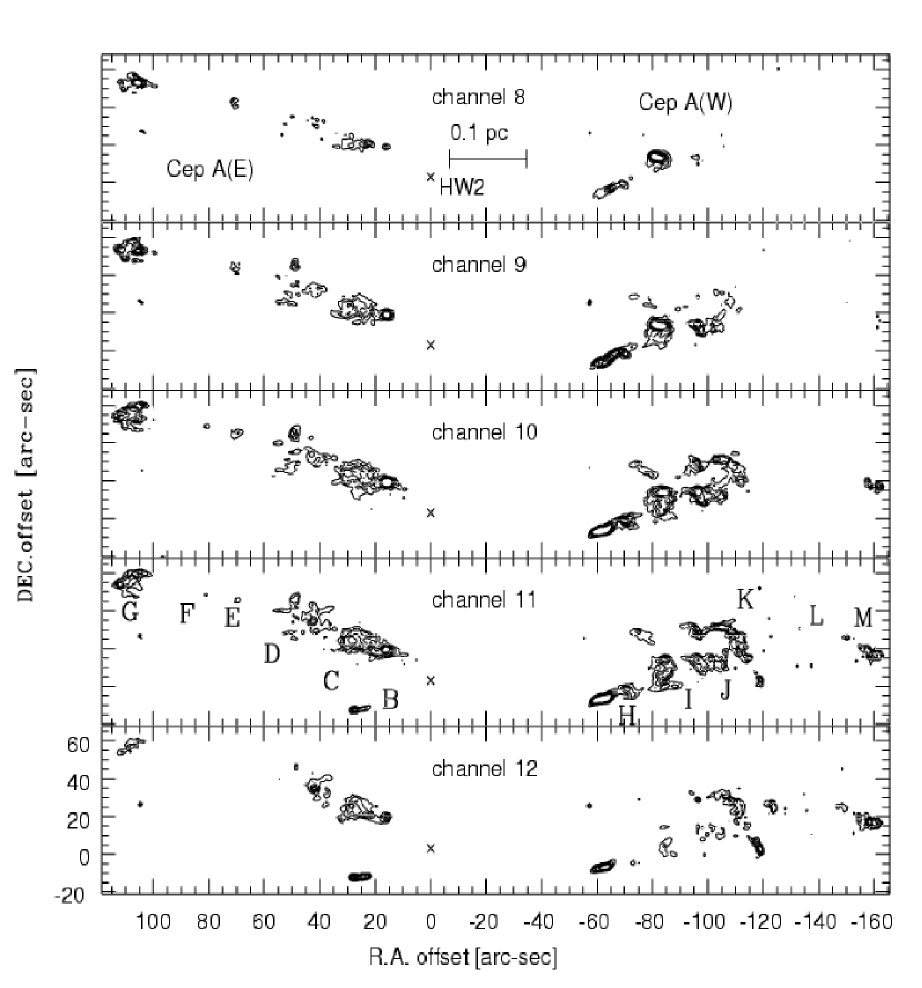
Figure 1: Velocity channel maps of the H₂ $v$=1–0 $S$(1) line emission in Cepheus A, showing the radial velocity structure of the two regions Cep A (E) and Cep A (W). The velocity varies from -42.1 km s^-1 in channel 8 (top) to -2.9 km s^-1 in channel 12 (bottom), the channel width is 9.8 km s^-1. The scale of the region is shown at the top panel. The contour intervals indicate the emission intensity in the range of 0.54 to 1.5 counts/sec and have the same increment values of 0.2 counts/sec. The cross indicates the position of the 6 cm peak of HW2 at R.A. = 22h45m17.9s and DEC. = +62° 01′ 49″  (2000), see Hughes & Wouterloot (1984). Offsets are referred to this reference position.

We created a color coded velocity image from the three channel velocity maps with more copious emission (-32.3, -22.5, and -12.7 km s^-1) as blue, green, and red respectively. Figure 2 presents this color composite map. It should be noted that these velocities are somewhat bluer than the -11.2 km s^-1 systemic velocity found from millimeter wavelength line observations of CO (e.g. Narayanan & Walker (1996)), as had already been noted by Doyon & Nadeau (1988).

The velocity structure in both regions shows a very complex pattern. However, a slightly systematic change from blue to red starting at the center of the image can be appreciated on the western outflow, that is not present in the eastern region. On the other hand, the Ceph A (E) region shows a large amount of small clumps with different velocities lying side by side.

We have calculated the centroid radial velocity for each pixel by taking only 10 velocity channels around the peak intensity. Figure 3 presents histograms of centroid radial velocity for the two H₂ emission regions of the image in Fig. 2. Regardless of the difference in morphology for the two regions, they have similar fractional distribution of pixels for a given radial velocity. However, Cep A (W) has a wing that extends into positive radial velocities and a small peak in the negative velocities.

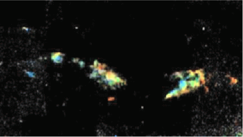
Figure 2: Color composite of the doppler shifted H₂ line emission $v$=1-0 $S$(1) in Cepheus A, showing the two main regions Cep A (E) and Cep A (W). Colors correspond to velocities in the LSR: Blue -32.3 km s^-1, green -22.5 km s^-1, and red -12.7 km s^-1. The region shown is about 5′$\times$3′, North is at the top and East is to the left.

Figure 3: Fraction of pixels with a given value of the centroid radial velocity (LSR) for the Cep A (E) (dashed line) and Cep A (W) (solid line) regions. The size of the bins is 2 km s^-1.

Figure 4 presents the centroid radial velocity as a function of displacement along the right ascension axis for both regions Cep A (E) and Cep A (W). All the channels with detected emission of H₂ from Fig. 2 are shown. The radial velocity of Cep A (E) has an almost constant mean value of $\sim$-18 km s^-1 along the region with a high dispersion around this value. Meanwhile, radial velocity of Cep A (W) increases its value with offset position to the West. We have fitted a line to each position-velocity data for each region and found rms residual values of 8.3 and 10.2 km s^-1 for Cep A(W) and Cep A(E), respectively. The smaller velocity dispersion and the large number of small clumps with different velocities (see Fig 2) in the East region indicate a more turbulent outflow in Cep A(E) compared to Cep A(W).

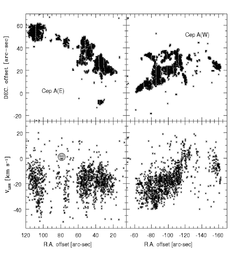
Figure 4: Diagrams of detected H₂ $v$=1–0 $S$(1) line emission in all velocity channels(top) and the velocity-position diagrams (bottom) for Cep A (E) (left) and Cep A (W) (right). Offset values are referred to the position of HW2 (see Fig. 1) considered as position (0,0).

3.2 A Mach disk in CephA(E)

The Cep A (E) outflow culminates in an arc shaped structure (labeled G in Fig. 1) that resembles a bow shock. This region is amplified in Fig. 5a. A bright spot can be seen in the center of the bow. The centroid velocities corresponding to this region are shown in Fig. 5c. The highest blue-shifted velocity of the region (-40 km s^-1) corresponds to a slightly elongated region (in the direction perpendicular to the outflow) that includes the bright spot and decreases toward the bow, as can also be seen in a position-velocity diagram in Fig. 5d. This kinematic behavior is expected if the bright spot corresponds to the Mach disk of the jet, where the jet material interacts with previously swept material accumulating in front of the jet and behind the bow shock.

A few cases are known where a Mach disk is observed in H₂. The case of Kumar et al. (2002) at the N1 outflow in S233IR (Porras et al., 2000), where a flattened structure is seen in high definition H₂ images, although it is not supported spectroscopically. In HH 7 Khanzadyan et al. (2003) detect a flattened [FeII] structure that coincides with a blue-shifted knot in H₂. This case is similar to the present case for Cep A (E). Blue-shifted velocity is expected as the jet material flows in all directions upon interacting at the Mach disk, in particular toward the present direction of the observer, nearly perpendicular to the outflow axis. As noted by Kumar et al. (2002) a detection of a Mach disk has rather interesting implications: 1) the jet would be partially molecular; 2) the velocity of the jet must be small enough to prevent dissociation of H₂ in the Mach disk; and 3) the jet should be heavy. In this case we can estimate the velocity of the molecular jet from the maximum observed velocity (-40 km s^-1) minus the rest velocity of the molecular cloud ($V_{0}$=-11.3 km s^-1) to be around 29 km s^-1. The distance from the Mach disk to the bow-shock apex is 5″  to 8″  ($\sim$0.016 to 0.025 pc at D=725 pc).

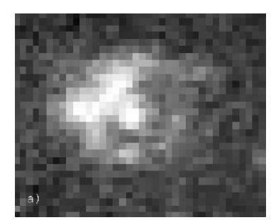
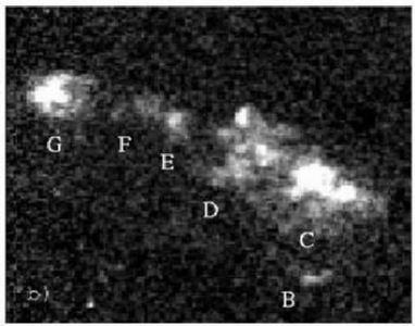
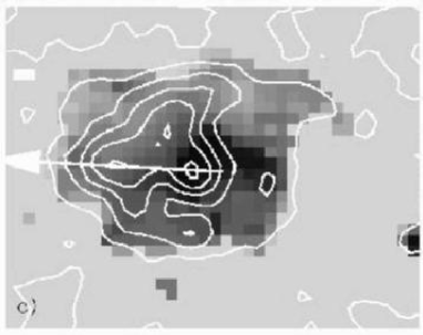
Figure 5: Mach disk in Cep A (E). (a) Amplified H₂ image of region G showing the edge of the outflow presented in panel (b). (c) shows the centroid velocity of the bow-shock region G in gray scale, going from $-40$ km s^-1 (black) to 0 km s^-1 in white. Overlaid contours show the intensity map. (d) shows a position-velocity diagram of a cut shown in (c) in the direction indicated by the arrow. The solid line corresponds to velocity $-(V-V_{0})$, $V_{0}=-11.3$ km s^-1, and the dotted line is intensity.

3.3 Cep A (W) velocity gradients

The western H₂ outflow in Cep A displays a series of wide arcs reminiscent of thin sections of shells. The outflow has been described as a hot bubble (Hartigan, Morse, & Bally, 2000) that drives C-shocks into the surrounding medium. In some shock fronts along this outflow, they observed that H₂ emission leads the optical [SII]$\lambda$6717 which in turn leads H$\alpha$. This is taken as evidence in favor of a C-shock that slowly accelerates and heats the ambient medium ahead of the shock. We find further evidence of this from the H₂ kinematics. A velocity gradient from higher to lower velocities is observed in some of the individual arc structures, as is the case for the one labeled I in Fig. 1. The spatial map of the centroid velocities in Cep A (W) is shown in Fig. 6. A smooth velocity gradient, covering from -36 km s^-1 to -8 km s^-1, is observed in the SW border of the arc, in the direction indicated by the arrow. That is, a velocity gradient going from blue-shifted to closer to the rest velocity of the molecular cloud (-11.2 km s^-1) in a region of 17″, or 0.06 pc at D=725 pc. We regard this as the kinematic evidence of a C-shock, as the slow acceleration of material ahead of the shock is quite evident.

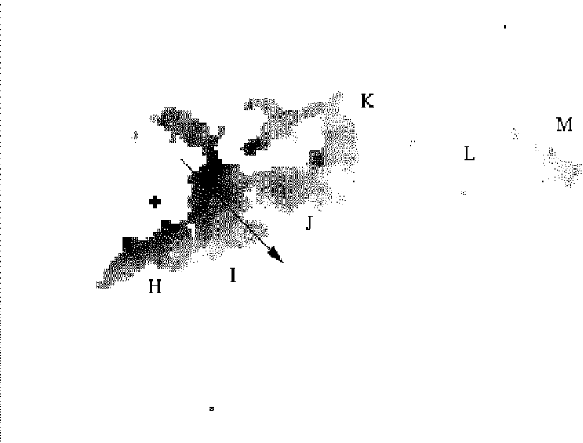
Figure 6: Velocity gradients in Cep A (W). The gray levels show velocity in the range -40 km s^-1 (black) to -4 km s^-1 (white).

3.4 Flux–velocity Relation

We have calculated the flux-velocity diagrams separately for the Cep A (E) and Cep A (W) outflows, as described in Salas & Cruz-González (2002). For every pixel with signal above the detection threshold, we added the fluxes of all the pixels with centroid velocities in bins of observed centroid velocity $\left|v_{obs}\,-\,v_{rest}\right|$, with respect to the rest velocity of the region (-11.2 km s^-1). The flux-velocity diagrams so obtained are shown in Fig. 7 and 8.

As shown by Salas & Cruz-González, this procedure gives similar flux-velocity relations for a variety of outflows, consisting in a flat spectrum for low velocities, followed by a power-law decrease above a certain break-velocity. The power-law index is very similar for different outflows, as is the case for Cep A (E) and Cep A (W) where it is -2.6$\pm$0.3 and -2.7$\pm$0.9 respectively (solid lines in figures 7 and 8). The break velocity however, is a little different. The logarithm of $v_{break}$ (in km s^-1) takes values of 0.95$\pm$0.07 and 1.13$\pm$0.13 respectively, a difference of around 2$\sigma$ which suggests that $v_{break}$ may be larger for Cep A (W). As was discussed in Salas & Cruz-González (2002), outflows of different lengths ($l$) show break-velocities varying as $v_{break}\propto l^{0.4}$, a result that is taken to imply an evolutionary effect, similar to the case of CO outflows (Yu et al., 1999). However, in the case of Cep A (E) and Cep A (W) the outflow length is very similar, as might be the outflow age. Salas & Cruz-González also argue that other causes for a difference in break velocities could be the amount of turbulence in the outflow, which might be the case for Cep A as is mentioned at the end of §3.1. We will next explore this possibility through the use of a wavelet analysis.

Figure 7: Flux-velocity relation of H₂ $v$=1–0 $S$(1) line emission in Cep A (E). The long-dashed line shows the flat low velocity behavior up to a break velocity where the solid line indicates a power law decrease. The dashed lines show the range of possible values of the index (-2.6$\pm$0.3) and of $log(v_{break})$ (0.95$\pm$0.07).

Figure 8: Same as in Fig. 7, but for the region Cep A (W). The range of possible values of the power law index is -2.7$\pm$0.9 and of $log(v_{break})$ is 1.13$\pm$0.13.

4 Wavelet Analysis of the H₂ emission from Cep A

4.1 Description

Both H₂ emission regions in Cep A show a rather complex velocity-position structure (see Fig. 2). We have carried out a wavelet analysis in an attempt to understand the relation between sizes of clumps, velocity, and velocity dispersion as a function of position along the outflows.

The wavelet transform analysis has been used before by Riera et al. (2003) to analyze H$\alpha$ observations using a Fabry-Pérot of the complex outflow in the HH 100 jet. Although, their procedure is equivalent to the one followed by Gill & Henriksen (1996) to study turbulence in molecular clouds, we have followed the analysis by Riera et al. (2003) because it is more relevant to the study of outflows.

The two-dimensional wavelet transform analysis is used to obtain the positions of all H₂ emission clumps as well as their characteristic sizes. The sizes of these clumps are determined from total H₂ flux images created by adding the continuum subtracted intensities of all the channel maps. Once obtained the positions and characteristic sizes of the H₂ structures of Cep A, the spatial averages (over the characteristic sizes of the structures) of the line center velocity and of the line widths are calculated to study the turbulence in the two regions of Cep A.

Our case is similar to Riera et al. (2003) in the sense that Cep A regions have an axial symmetry and that the kinematics properties seem to depend on the offset along this axis. Then, it is reasonable to expect that the characteristic size may be different along and across the regions. To exploit this symmetry, we rotated the H₂ image so the long part of both regions, the main axis, is parallel to the $x$ coordinate defined along the east-west direction. On this rotated images, we carried out an anisotropic wavelet decomposition using two bases of different sizes, one along and one across the main axis.

We adopted a basis of “Mexican hat” wavelets of the form

$$g(r;a_{x},a_{y})=C(2-r^{2})e^{-r^{2}/2}\;,$$ (1)

where $r=[(x/a_{x})^{2}+(y/a_{y})^{2}]^{1/2}$; $a_{x}$ and $a_{y}$ are the scale lengths of the wavelets along the $x$- and $y$-axes, respectively, and $C=(a^{2}_{x}+a^{2}_{y})^{-1/2}$. This is a very common used wavelet, but we also choose to use it because simplifies the detection of intensity peaks, approaches better to the shape of the intensity peaks, and behaves well under FFT calculations.

To compute the wavelet transform we have to calculate the convolutions

$$T_{a_{x},a_{y}}(x,y)=\int\int I(x^{\prime},y^{\prime})g(r^{\prime};a_{x},a_{y})dx^{\prime}dy^{\prime}\;,$$ (2)

for each pair ($a_{x},a_{y}$), where $r^{\prime}=\{[(x^{\prime}-x)/a_{x}]^{2}+[(y^{\prime}-y)/a_{y}]^{2}\}^{1/2}$, $I(x,y)$ is the intensity at pixel position $(x,y)$, and $g(r^{\prime};a_{x},a_{y})$ is give by eq. (1). These convolutions are calculated by using a Fast Fourier Transform (FFT) algorithm (Press et al., 1992).

The wavelet transformed images $T_{a_{x},a_{y}}(x,y)$ correspond to smoothed versions of the intensity of the H₂ image. We use this images to find the sizes of the structures in the H₂ regions of Ceph A. First, on the transformed image with $a_{x}=a_{y}=1$, we fixed the position of $x$ and find all the values of $y$ where $T_{a_{x},a_{y}}(x,y)$ has a local maximum. Several maxima may be found for each position $x$ that correspond to different structures observed across the regions. The maxima found with $a_{x}=a_{y}=1$ will correspond also to the local maxima of $I(x,y)$.

For each pair ($x$,$y$) where $I(x,y)$ has a maximum we determine $(a_{x},a_{y})$, in the $a_{x}$ and $a_{y}$ space, where the wavelet transform has a local maximum. $a_{x}$ and $a_{y}$ will be the characteristic size of the clump with a maximum intensity at ($x$,$y$). The ($a_{x}$,$a_{y}$) space is search in such way that we first identify the size of the smaller clumps and then the bigger ones. This progressive selection allow us avoid to choose clumps that overlap with its neighbors. Naturally, the biggest clumps will have an structure similar to the whole region.

4.2 Size of the H₂ Clumps

The results obtained with the process described above are shown in Fig. 9. This figure shows the two images of molecular hydrogen emission of Cep A, which have been rotated by 19$\arcdeg$ so the longways dimension of the regions are more or less parallel to the $x$-axis. In the case of Cep A (E), the $x$ axis has been also inverted (West is to the right) so the $x$ values in both panels in Fig. 9, although arbitrary in origin, are an estimate of the offset from the central region between the two regions. It has to be clarified that the $x$ coordinates are values from independent images so there is really no correlation between them. However, the span in the vertical and horizontal axis are kept the same in both panels of Fig. 9 to ease the size comparison for each region. Six large structures (B to G) were identified in Cep A (E) and six (H to M) for Cep A (W) (see Fig. 1). The spatial limits of these regions are shown in Table 1.

Table 1: H₂ Emission Regions in Cep A

Region	$x_{min}$	$x_{max}$	$y_{min}$	$y_{max}$	$m$	$\alpha$
B	72	88	102	115	0.612	-0.073:
C	53	91	129	159	0.774	0.140
D	92	119	133	170	0.702	0.169
E	127	140	142	158	0.739	0.155:
F	140	153	144	155	0.394	0.644
G	163	199	132	160	0.768	0.249
H	67	92	129	144	–	0.397:
I	92	110	129	155	0.871	-0.089:
J	113	129	132	147	0.654	0.563
K	130	142	115	162	–	0.379
L	142	187	115	150	0.931	0.439
M	188	206	113	131	0.937	0.376

The H₂ intensity maps have then been convolved with a set of wavelets $g(r;a_{x},a_{y})$ with $1\leq a_{x}\leq 30$ pixels and $1\leq a_{y}\leq 30$ pixels for Cep A (E) and $1\leq a_{x}\leq 35$ pixels and $1\leq a_{y}\leq 35$ pixels for Cep A (W), with a resolution of 0.853 arc-sec per pixel in the $x$-direction and 0.848 arc-sec per pixel in the $y$-direction. The upper limiting values for $a_{x}$ and $a_{y}$ were selected to allow very few overlapping in the size of the regions in adjacent peaks.

The values of the peaks $y_{k}$ of the wavelet transform obtained for each position $x$ along the region are shown in the bottom panel of Fig. 9. Also shown as error bars are the values of $a_{x,k}$ and $a_{y,k}$ corresponding to each peak, which give an estimate of the characteristic sizes along and across the observed structures.

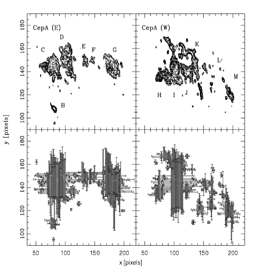
Figure 9: Position and characteristic sizes of the structures (bottom) and contour plots of the H₂ image (top) obtained from the velocity channels for Cep A (E) (left) and Cep A (W) (right). Contour levels shown from 0.0 to 1.5 counts/sec in 0.1 counts/sec increments for both plots. The plus sign shows the positions of the maximal $y_{k}$ of the wavelet transform obtained for the different values $x$ along the region. The characteristic sizes $a_{x,k}$ and $a_{y,k}$ of these maximal are shown as error bars centered on the positions of the maximal. We have separately rotated the map of each region by 19^∘ so they are more or less parallel to the $x$-axis. The distances $y$ (across the regions) and $x$ (along the regions), in pixels units, are with respect to the rotated image and have an arbitrary origin. In the Cep A (E) case the $x$ axis has been inverted (West is to the right) for analysis purpose (see text).

To quantify the observed broadening of the region, for each position $x$ we compute the weighted mean of the $y$-spatial scale perpendicular to the longest axis of the regions:

$$\langle a_{y}\rangle=\frac{\sum_{k}a_{y,k}T_{a_{x,k},a_{y,k}}(x,y_{k})}{\sum_{k}T_{a_{x,k},a_{y,k}(x,y_{k})}}\;.$$ (3)

Figure 10  shows $\langle a_{y}\rangle$ as a function of position $x$ along the two Cepheus A regions. In both outflows we notice the presence of small (2 pixels) and large (25 pixels) structures located with no discernible order along the axial position.

Figure 10: Values of $\langle a_{y}\rangle$ plotted as a function of position $x$ along the Cep A (E), top panel, and Cep A (W) at the bottom one.

The values of $a_{y,k}$ as a function of $a_{x,k}$ are shown in Fig. 11 Cep A (E) and Cep A (W). These graphs represent a measure of the symmetry of the structures. Isotropic structures are expected to attain $a_{y,k}=a_{y,k}$ and should thus be located on a line of unitary slope. The values of the slope $\alpha$ for each region are also given in Table 1. We note that all the values are in general less than one, indicating structures that are longer than wider. The western outflow, however, shows relatively wider structures than Cep A (E), a property which has also been qualitatively observed. It may be possible that the individual structures follow the pattern of each region as a whole, with the eastern region being longer than wider while the western region is the opposite. However, the nature of these anisotropies it is not clear.

Figure 11: Left: Values of $a_{y,k}$ plotted as a function $a_{x,k}$ for the different regions along Cep A (E). The linear fits to the points are drawn as solid lines. The slope $m$ of the linear fit is listed in Table 1. Right: Same but for the region Cep A (W).

4.3 Spatial distributions of the radial velocities and the line widths

In this section we describe the spatial dependence of the kinetic properties of the two main H₂ emission regions of Cep A.

From the cube of position-velocity data, we calculate two moments of the line profiles for each pixel:

$$V_{c}=\frac{\int vI_{v}dv}{\int I_{v}dv}\;,$$ (4)

and

$$W^{2}=\frac{\int(v-V_{c})^{2}I_{v}dv}{\int I_{v}dv}\;.$$ (5)

In these equations, $v$ is the radial velocity, and $I_{v}$ the intensity at a fixed position $(x,y)$ of successive channel maps. The integrals are carried out over all the velocity channel maps. Here $V_{c}$ is the barycenter of the line profile (i.e. the “line center” radial velocity), and $W$ is a second-order moment that reflects the width of the line profile.

With these values of $V_{c}$ and $W$ computed for all positions $(x,y)$ on the plane of the sky, we calculate the following spatial averages (Riera et al., 2003):

$$\langle V_{c}\rangle=\frac{\int_{S_{a_{x},a_{y}}}V_{c}(x^{\prime},y^{\prime})I(x^{\prime},y^{\prime})dx^{\prime}dy^{\prime}}{\int_{S_{a_{x},a_{y}}}I(x^{\prime},y^{\prime})dx^{\prime}dy^{\prime}}\;,$$ (6)

$$\langle W^{2}\rangle=\frac{\int_{S_{a_{x},a_{y}}}W^{2}(x^{\prime},y^{\prime})I(x^{\prime},y^{\prime})dx^{\prime}dy^{\prime}}{\int_{S_{a_{x},a_{y}}}I(x^{\prime},y^{\prime})dx^{\prime}dy^{\prime}}\;,$$ (7)

$$\langle\Delta v^{2}\rangle=\frac{\int_{S_{a_{x},a_{y}}}[V_{c}(x^{\prime},y^{\prime})-\langle V_{c}\rangle]^{2}I(x^{\prime},y^{\prime})dx^{\prime}dy^{\prime}}{\int_{S_{a_{x},a_{y}}}I(x^{\prime},y^{\prime})dx^{\prime}dy^{\prime}}\;,$$ (8)

where $I(x^{\prime},y^{\prime})$ is the H₂ flux obtained from co-adding all the channel maps. These integrals are carried out over areas $S_{a_{x},a_{y}}$ which are ellipses with central positions ($x,y$) and major and minor axes, $a_{x}$ and $a_{y}$, corresponding to all the values that have been identified as peaks of the wavelet transform.

The value of $\langle W^{2}\rangle(x,y)$ corresponds to the line width spatially averaged over the ellipse $S_{a_{x}a_{y}}$ with a weight $I(x^{\prime},y^{\prime})$. The same weight spatial average is calculated for the line center velocities $\langle V_{c}\rangle$ within the ellipse, as well as the standard deviation $\langle\Delta v^{2}\rangle^{1/2}$ of these velocities.

Figure 12 shows the line centers, widths, and standard deviations as a function of position $x$ along the region (all of the points at different positions $y$ across the region and with different $a_{x}$ and $a_{y}$ are plotted). The line center or centroid velocity displayed in the top panels, shows different behaviors for Cep A (E) and Cep A (W). As had been previously noted, Cep A (E) has a constant velocity along the outflow ($\sim$-19 km s^-1) while Cep A (W) shows a velocity gradient from about -21 to -2  km s^-1. A large dispersion in the line centers for Cep A (W) around positions 115 and 162 is probably due to insufficient S/N, since a similar increase in the dispersion velocity (medium panel) is concurrent, but lacks a corresponding increment of the line width (bottom panel). Other features present in these figures seem real. Most remarkably, the velocity dispersion (medium panel) for Cep A (E) increases monotonically with distance from the source, going from around 4 to 10 km s^-1 in 150 pixels or 0.5 pc. No such increase is observed in the western outflow, where we obtain a constant 3$\pm$2 km s^-1 velocity dispersion. The line widths (bottom panel) seem dominated by the width of the instrumental profile of 22 km s^-1.

Hence, we conclude from this analysis that the eastern and western outflows seem intrinsically different. While the eastern outflow shows a constant line center velocity and an increasing velocity dispersion, the western outflow behaves otherwise, showing a velocity gradient and a constant velocity dispersion with a lower value. This had been noticed in our qualitative analysis of the observations. Now, if we take the velocity dispersion within each cell as a measure of turbulence, which seems reasonable, then the region Cep A (E) is more turbulent than Cep A (W), and it is noticeable that the turbulence increases with distance from the “central” source compared to a constant behavior in the western source.

Figure 12: Average line centers (top panels), standard deviations (middle), and line widths (bottom) as a function of position $x$ along the regions Cep A (E) (left column) and Cep A (W) (right column). All points with different positions $y$ across the region and with different $a_{x}$ and $a_{y}$ are plotted.

4.4 Deviations of the line center velocity and the size of the region

Figure 13 shows the deviations of the line center velocity (velocity dispersion), averaged over sizes chosen from the wavelet spectrum, as a function of the size of each region. Such deviations of the line center velocity, averaged over sizes chosen from a wavelet spectrum, have been previously used by Gill & Henriksen (1996) to study turbulence in molecular clouds. In this figure we can appreciate a large dispersion of values. However, points tend to clump together around certain regions of the diagrams.

A closer examination of Fig. 13 for Cep A (E) shows a cluster of points at position (20,9) corresponding to structure labeled G (see Fig. 9), while the points corresponding to structure C lie just below of them. Taken separately, each one of these groups seem to define a line in the diagram, offset vertically from one another, but of comparable slopes. The slope of the lines, in fact, is also similar to the slope of the line that would be obtained by fitting a line to all the data, $m$=0.26 (indicated with a solid line in Fig. 13). The dispersion is large, but there is at least another factor contributing to the amount of velocity dispersion that has already been mentioned: the distance from the components of the structure to the outflow source. We take out this effect by subtracting this systematic linear contribution with the distance. Thus, in Fig. 13, points belonging to the C group, which are closer to the source, would merge together with those points of the farther G group. The dispersion would be lower and the slope would have a similar value. This defines a relation similar to Larson’s law for molecular clouds (Larson, 1981). Larson found that molecular clouds show a suprathermal velocity dispersion that correlates with the size $a$ of the cloud as $\sigma_{v}\propto a^{0.38}$. Although different values of the power index, $\alpha$, have been mentioned in the literature, ranging from 0.33, for pure Kolmogorov turbulence, to 0.5, a more appropriate value in terms of the Virial Theorem (Goodman et al., 1998). In the Cep A (E) case we obtain a slope $\alpha$ of 0.25 which is closer to the Kolmogorov value.

In the western outflow it is more difficult to identify clumps of points, and we were not able to find a relation of velocity dispersion with position either. A least square fit of a line to the data gives a slope of 0.20. However, there appears to be two disperse clumps of points, a lower one and an upper one, each defining a line with a larger slope $\alpha\sim$0.5 and parallel to each other. This latter value would be closer to a case where Virial Theorem applies.

The analysis of the individual H₂ condensations (c.f. Fig. 1) in the Cep A (E) and Cep A (W) is illustrated in Fig. 14 and 15. We show the deviations for the line center velocity, averaged over sizes chosen from the wavelet spectrum for each condensation. For each H₂ condensation the values of the best fit slope $\alpha$ are presented in the last column of Table 1. The Cep A (E) clumps yield a mean $\alpha$ of 0.21$\pm$0.21 while the Cep A (W) yield a slightly higher value of 0.34$\pm$0.20. However, some knots show poor correlations than others (see plots for knots B, E, H and I). Using only knots C, D, F and G for Cep A (E) and knots J, K, L and M for Cep A (W) yields an $\alpha$ of 0.30$\pm$0.20 and 0.44$\pm$0.08, which support a Kolmogorov case in the first and a more virialized region for the western case.

Figure 13: Relation of the deviations of the line center velocity, $\langle\Delta v^{2}\rangle^{1/2}$ (or $\sigma$), averaged over regions chosen from the wavelet spectrum, and the size $a$ of the region, $(a_{x}^{2}+a_{y}^{2})^{1/2}$, for the complete Cep A (E) (left) and Cep A (W)(right) regions. The solid line is the best fit to the points with a slope $\alpha$ of 0.2574 for Cep A (E) and 0.199 for Cep A (W).

Figure 14: Relation of the deviations of the line center velocity, averaged over regions chosen from the wavelet spectrum, $\langle\Delta v^{2}\rangle^{1/2}$, and the size of the region $a_{x}^{2}+a_{y}^{2})^{1/2}$ for regions B to G of Cep A (E). The solid line is the best fit to the points. The values of the slope $\alpha$ of the fits are given in the last column of Table 1.

Figure 15: Relation of the deviations of the line center velocity, averaged over regions chosen from the wavelet spectrum, $\langle\Delta v^{2}\rangle^{1/2}$, and the size of the region $(a_{x}^{2}+a_{y}^{2})^{1/2}$ for regions H to M of Cep A (W). The solid line is the best fits to the points. The values of the slope $\alpha$ of the fits are given in the last column of Table 1.

5 Conclusions

We have presented the velocity structure of the molecular hydrogen outflows from the regions Cep A (E) and Cep A (W) obtained from the H₂ $v$=1–0 $S$(1) doppler shifted line emission at 2.12 $\mu$m. Both the velocity channel maps and the integrated H₂ image show a complex structure of 12 individual clumps along two separated structures oriented roughly in the east-west direction.

Given the complexity of these structures, we have carried out an anisotropic wavelet analysis of the H₂ image, which automatically detects the position and characteristic sizes (along and across the region axis) of the clumps.

1. There is evidence for a Mach disk in Cep A (E). The efflux point is located at the center of a bow shock structure and we measure blue-shifted velocities of 22 to 28 km s^-1. This observation implies that a molecular jet is driving the outflow.

2. Cep A (W) on the other hand, is consistent with a hot bubble in expansion driving C-shocks. We presented the kinematic gradient of one of such shocks as an example.

3. The H₂ flux-velocity relation is present in both outflows. The break velocity of the eastern outflow is lower than that of the western outflow, and we have argued that this is indicative of greater turbulence in Cep A (E).

4. The wavelet analysis has confirmed and quantified trends observed in the centroid velocity measurements: that the eastern outflow shows a constant line center velocity and an increasing velocity dispersion, while the western outflow shows a velocity gradient and a constant velocity dispersion. The larger velocity dispersion and gradient in the eastern outflow is taken as indicative of turbulence, and allows us to conclude also that turbulence increases with distance.

5. Suggestive propositions about the kind of turbulence present in both outflows, are extracted from an analysis of the relation of the velocity dispersion as a function of the size of the structures (cells) identified as unities by the wavelet spectrum. Using only knots with a good correlation yields an $\alpha$ of 0.30$\pm$0.20 for Cep A (E) and 0.44$\pm$0.08 for Cep A (W), which support a Kolmogorov case in the first and a more virialized region for the western case.

References

- Bally & Lane (1982) Bally, J., & Lane, A. P. 1982, ApJ, 257, 612
- Codella et al. (2003) Codella, C., Bachiller, R., Benedettini, M., & Caselli, P. 2003, MNRAS, 341, 707
- Cruz-González et al. (1994) Cruz-González, I., Carrasco, L., Ruiz, E., Salas, L., Skrutskie, M., Meyer, M., Sotelo, P., Barbosa, F., Gutiérrez, L. , Iriarte, A., Cobos, F., Bernal, A., Sánchez, B., Valdéz, J., Argüelles, S., Conconi, P.: 1994, Proc. SPIE 2198, p. 774.
- Doyon & Nadeau (1988) Doyon, R., & Nadeau, D. 1988, ApJ, 334, 883
- Garay et al. (1996) Garay, G., Ramírez, S., Rodríguez, L. F., Curiel, S., & Torrelles, J. M. 1996, ApJ, 459,193
- Gill & Henriksen (1996) Gill, A. G., & Henriksen, R. N. 1990, ApJ, 365, L27
- Goodman et al. (1998) Goodman, A. A., Barranco, J. A., Wilner, D. J. & Heyer, M. H. 1998, ApJ, 504, 223
- Hartigan, Morse, & Bally (2000) Hartigan, P., Morse, J., & Bally, J. 2000, ApJ, 120, 1436
- Hartigan et al. (1996) Hartigan, P., Carpenter, J., Dougados, C., & Skrutskie M. 1996, AJ, 111, 1278
- Hartigan, Raymond, & Hartmann. (1987) Hartigan, P., Raymond, J., & Hartmann, L. 1987, ApJ, 316, 323
- Hartigan et al. (1986) Hartigan, P., Lada, C., Stocke, J., & Tapia, S. 1986, AJ, 92, 1155
- Hartigan & Lada (1985) Hartigan, P., & Lada, C. J. 1985, ApJS, 59, 383
- Hughes & Wouterloot (1984) Hughes, V. A. & Wouterlloot, J. G. A. 1984, ApJ, 276, 204
- Johnson (1957) Johnson, H. L. 1957, ApJ, 126, 121
- Khanzadyan et al. (2003) Khanzadyan, T., Smith, M. D., Davis, C. J., Gredel, R., Stanke, T., & Chrysostomou, A. 2003, MNRAS, 338, 57
- Koppenaal et al. (1979) Koppenaal, K., Sargent, A. I., Nordh, L., van Duinen, R. J., & Aslders, J. W. G. 1979, A&A, 75, L1
- Kumar et al. (2002) Kumar, M.S.N., Bachiller, R., & Davis, C.J. 2002, ApJ, 576, 313
- Larson (1981) Larson, R. B. 1981, MNRAS, 194, 809
- Narayanan & Walker (1996) Narayanan, G., & Walker, C. K. 1996, ApJ, 466, 844
- Porras et al. (2000) Porras, A., Cruz-Gonzalez, I., & Salas, L. 2000, A&A, 361, 660
- Press et al. (1992) Press, W. H., Teukolsky, S. A., Vetterling, W. T., & Flannery, B. P. 1992, “Numerical Recipes in C”. Second Ed. Cambidge University Press
- Raines et al. (2000) Raines, S. N., Watson, D. M., Pipher, J. L.,; Forrest, W. J., Greenhouse, M. A., Satyapal, S., Woodward, C. E., Smith, H. A., Fischer, J., Goetz, J. A., Frank, A. 2000, ApJ, 528, L115
- Riera et al. (2003) Riera, A., Raga, C. A., Reipurth, B., Amram, P., Boulesteix, J., Cantó, J., & Toledano, O. 2003, AJ, 126, 327
- Rodríguez, Ho, & Moran (1980) Rodríguez, L. F., Ho, P. T. P, & Moran, J. M. 1980, ApJ, 240, L149
- Salas et al. (1999) Salas, L. et al. 1999, ApJ, 511, 822
- Salas & Cruz-González (2002) Salas, L., & Cruz-González, I. 2002, ApJ, 572, 227
- Simon & Joyce (1983) Simon, T., & Joyce, R. R. 1983, ApJ, 265, 864
- Sargent (1977) Sargent, A. I. 1977, ApJ, 218, 736
- Torrelles et al. (1993) Torrelles, J. M., Verdes-Montenegro, L., Ho, P. T .P., Rodríguez, L. F., & Cantó, J. 1993, ApJ, 106, 613
- Yu et al. (1999) Yu, K. C., Billawala, Y., & Bally, J. 1999, AJ, 118, 2940