Detecting and interpreting statistical lensing by absorbers

Abstract

We propose a method for detecting gravitational magnification of distant sources, like quasars, due to absorber systems detected in their spectra. We first motivate the use of metal absorption lines rather than Lyman-$\alpha$ lines, then we show how to relate the observed moments of the source magnitude distribution to the mass distribution of absorbers. In order to illustrate the feasibility of the method, we use a simple model to estimate the amplitude of the effect expected for MgII absorption lines, and show that their lensing signal might already be detectable in large surveys like the SDSS. Our model suggests that quasars behind strong MgII absorbers are in average brightened by $-0.05$ to $-0.2$ magnitude due to magnification. One must therefore revisit the claim that, in magnitude limited surveys, quasars with strong absorbers tend to be missed due to extinction effects. In addition to constraining the mass of absorber systems, applying our method will allow for the quantification of this bias.

1 Introduction

During the last decade, gravitational lensing has become an invaluable tool for constraining the mass of many different structures (exoplanets, stars, galaxies, clusters, large scale structure, etc.) and has significantly improved our knowledge of many of these systems. However, there have been very few results for absorption line systems, which is unfortunate because these objects present a number of interesting aspects: low-ionisation metal lines and strong HI lines sample the cold dense gas bound in galactic systems, independent of the galaxy luminosities. Moreover absorption-line measurements are largely insensitive to redshift and give us access to early stages of galaxy formation.
Gravitational lensing by absorbers has been investigated theoretically by a number of authors. So far all studies have focused on hydrogen line absorbers, which offer easier theoretical modeling than metal lines since complications due to gas metallicities can be avoided. For most of these investigations, lensing has been studied for its effects on quasar luminosity functions, i.e. the magnification bias, and on the observed distribution of impact parameters with respect to the center of the lenses (Pei 1995, Bartelmann & Loeb 1996, Smette et al. 1997, Hamana et al. 2000, Le Brun et al. 2000, Maller et al. 2002, Perna et al. 2002). However, only a few authors have used this technique to study the absorber systems themselves. Several studies have used multiple quasar images to probe the extent of gas clouds (Smette et al. 1995, Kobayashi et al. 2002, Ellison et al 2004), but in the context of absorbers, gravitational lensing has rarely been used to constrain the mass properties of the lenses, i.e. the purpose for which it is usually used. As far as we know, only Maller et al. (2002) have proposed a method to investigate the properties of an absorber population using lensing. They suggested analyzing the distribution of Lyman-limit systems as a function of column density, assuming that the corresponding unlensed distribution follows a power law, and they showed how to use the measured deviations to obtain a lower limit for the mass to gas column density ratio of these systems. Unfortunately, their method requires a very large number of quasars and has not been applied so far.

This general lack of observational results for absorber systems might originate in the preferential focus of previous studies on Lyman-$\alpha$ absorbers. Indeed, analytic models can be used more easily than for other absorption lines and strong systems like DLAs are expected to trace the inner part of dark matter halos and therefore favor gravitational magnification effects. However the quantity relevant to obtaining observational results is not simply the amplitude of lensing effects, but the signal-to-noise ratio of the detection that can be achieved. In such a case, strong Lyman-$\alpha$ absorbers might not be optimal candidates because large samples are difficult to build.

Whereas for damped Lyman-$\alpha$ absorbers theoretical studies exist but observational results are lacking, the situation is the opposite for metal absorbers: no theoretical prediction has been made so far but a few authors have attempted to detect magnification effects of metal absorber systems. The first observational approach was to fit lensing models to the redshift evolution of quasar absorbers to disentangle intrinsic evolution from gravitational lensing (Thomas & Webster 1990, Borgeest & Mehlert 1993); however, these studies could not find any signal from lensing. Another approach first suggested by York et al. (1991) was to divide a sample of quasar spectra into bright and faint subsamples in order to determine the incidence of metal absorbers (CIV, SiIV) in each subsample separately. However these authors found no clear evidence of gravitational lensing. Van den Berk et al. (1996) extended the analysis to a larger sample of quasar spectra compiled from the literature. They found an excess of CIV absorbers in luminous quasars but did not find a similar trend in the available MgII sample. More recently, Ménard & Péroux (2003) used the 2dF-Quasar survey to compare the number of quasars with and without absorbers as a function of magnitude. They found a relative excess of bright quasars with absorbers as well as indications of reddening effects. Finally, Ménard, Nestor and Turnshek have performed a more detailed analysis with data from the Sloan Digital Sky Survey (SDSS) and find similar results (Ménard et al., in preparation).
The variety of results obtained in all these analyses turn out to be rather difficult to interpret because the absorber species, redshift and equivalent width ranges differ. Moreover, as emphasized by Ménard & Péroux (2003), such analyses can easily be biased if the selection of the objects is not done carefully enough. For example, since absorption lines are more easily detected in high signal-to-noise ratio spectra and since these tend to correspond to bright quasars, a naive absorption line selection would introduce systematic magnitude shifts. In addition, the lack of theoretical estimates did not allow for any guidance in interpreting the existing observational results.

In this paper we present the first calculation of statistical magnification effects due to metal absorbers and investigate the possible constraints on the absorber mass distribution. In section 2 we first motivate the use of metal absorption lines, which possess a number of properties better suited for statistical analyses than Lyman-$\alpha$ lines. Then we present a method for extracting the signal expected from gravitational magnification and show how to use it to constrain the mass distribution of these systems. In section 3, in order to demonstrate the feasibility of this technique, we use recent data on MgII systems, along with a simple lensing model to estimate the amplitude of the expected effects. Finally, we estimate the corresponding noise level in section 4 and show that the SDSS might provide the necessary data for a detection.

2 Detecting the statistical magnification of quasars

2.1 The choice of absorption lines

Narrow metal absorption lines and damped Lyman-$\alpha$ lines found in quasar spectra are usually believed to indicate the presence of a galaxy along the line-of-sight (Bahcall & Spitzer 1969). In some rare cases, in which the absorbing galaxy is massive enough and the impact parameter is less than a few kpc, such a source-lens-observer configuration can give rise to multiple quasar images (see for example Turnshek et al. 1997). However, most often when absorption lines are detected in a quasar spectrum, such configurations are not encountered and lensing modifies the magnitude of the source without producing additional images. Measuring these lensing effects can then only be done in a statistical sense, because we do not know a priori the intrinsic magnitude of a given background quasar. A large sample of quasars and absorber systems is therefore required in order to detect the magnification due to absorbers.
As mentioned in the Introduction, gravitational lensing by strong Lyman-$\alpha$ absorbers has already been investigated theoretically by a number of authors, motivated by the fact that such absorption features trace the inner part of galactic halos and are therefore expected to favor gravitational lensing effects. Unfortunately, Lyman-$\alpha$ lines can only be seen at redshifts $z\gtrsim 2$ from the ground so that only a small fraction of observed quasars can allow for their detection. It is thus difficult to build a large sample of such absorption lines. Another drawback related to the high redshift ranges comes from the fact that the lensing efficiency drops if both lenses and sources are located at $z\gtrsim 2$.

The statistical nature of the problem and the redshift ranges involved motivate the use of metal lines. Given the large range of possible absorption wavelengths they can be found at various redshifts from the ground, they can therefore be selected in order to maximize the lensing efficiency, and they probe a large range of galactic impact parameters, from a hundred kpc down to a few kpc. Therefore metal lines appear to be more appropriate than Lyman-$\alpha$ lines for the purpose of detecting statistical magnification effects. The method presented below can be applied to absorption lines like MgII, FeII, SiII, CIV, etc. In section 3 we will explore its feasibility by estimating the signal expected in the case of MgII absorption lines. Their 2796,2803 $\mathrm{\AA}$ doublet can be observed from the ground over a very large range of redshifts ($0.2\leq z\leq 2.2$), they are astrophysically abundant, and they have been seen to be very close tracers of optically thick H I gas (Bergeron & Stasinska 1986). We will consider strong MgII absorbers, i.e. with a rest equivalent width $W_{0}\gtrsim 0.3\;\mathrm{\AA}$. Such systems can be detected with the relatively low spectroscopic resolutions $(\mathrm{R}\sim 2000)$ used in current large surveys like 2dF and SDSS.

2.2 Extracting the signal

The presence of a galaxy close to the line-of-sight of a background source can modify its brightness in two ways: first, it can act as a gravitational lens and amplify the flux of the source and second, the presence of dust around the galaxy can extinct and redden the source’s light. This can be described by

$$\mathrm{f}(\lambda)=\mathrm{f}_{\mathrm{ref}}(\lambda)\,e^{-\tau(\frac{\lambda}{1+z_{\mathrm{a}}})}\times\mu\leavevmode\nobreak\ ,\leavevmode\nobreak\ \leavevmode\nobreak\ \leavevmode\nobreak\ \leavevmode\nobreak\ \leavevmode\nobreak\ \leavevmode\nobreak\ \leavevmode\nobreak\ \leavevmode\nobreak\ \leavevmode\nobreak\ \leavevmode\nobreak\ \leavevmode\nobreak\ \leavevmode\nobreak\ \leavevmode\nobreak\ \leavevmode\nobreak\ \leavevmode\nobreak\$$ (1)

where $\mathrm{f}(\lambda)$ is the altered flux of a source behind an galaxy, $\mathrm{f}_{\mathrm{ref}}(\lambda)$ is the flux that would be observed without intervening system, $\tau_{\lambda}$ is the optical depth of the galaxy and $\mu$ its gravitational amplification. The corresponding magnitude change can then be written

$$\delta m = m-m_{\mathrm{ref}}$$ (2)

$$= -2.5\,\log(\mu)+\frac{2.5}{\log e}\,\tau(\frac{\lambda}{1+z_{\mathrm{a}}})\;.$$

Whereas gravitational magnification is achromatic, extinction effects strongly depend on wavelength and usually become small in near infrared bands. In this paper we will focus on magnification only, arguing that observations at appropriate wavelengths can isolate the lensing effects. Below, it will be shown how to get constraints on dust extinction of metal absorbers using the proposed measurements.

Let us consider an area of the sky which is large enough for the mean magnification to be close to unity. In this area, let us consider a population of sources, with a fraction of them being lensed. Let $\mathrm{N_{ref}}(m)$ be the intrinsic magnitude distribution of the the unlensed sources and let $\mathrm{N_{lens}}(m)$ be that of the lensed ones. Let $f$ be the fraction of sources behind a lens and $\mathrm{P}(\delta m)$ be the distribution of magnitude shifts induced by these systems. We then have the following relation between the magnitude number counts:

$$\mathrm{N}_{\mathrm{lens}}(m)=f\times\int\mathrm{N}_{\mathrm{ref}}(m-\delta m)\;\mathrm{P}(\delta m)\;\mathrm{d}(\delta m)\leavevmode\nobreak\ .$$ (3)

If the lenses can be counted independently from the sources, $f$ can then be estimated separately and information on the magnification properties of the lenses, i.e. the distribution $\mathrm{P}(\delta m)$, can be extracted from the observed number of lensed sources at a given magnitude. This information has been the one measured for example in the case of quasar-galaxy correlations induced by lensing. In such a case, the magnification bias changes the number density of background sources angularly close to foreground lenses (see for example Bartelmann & Schneider 2001). However, if lenses cannot be observed independently from their background sources, as is the case for systems seen in absorption, a degeneracy exists between the intrinsic number of lenses and the amplitude of the magnification bias, at a given magnitude. As shown in Eq. 3, increasing the fraction of lenses $f$ or increasing their magnification, i.e. $-\delta m$, produce similar effects at a given magnitude. Therefore, probing lensing effects must be done by measuring changes in the shape of the magnitude distribution of the lensed population, $\mathrm{N_{lens}}(m)$, with respect to that of the reference population $\mathrm{N_{ref}}(m)$. In the following we will estimate this effect in the context of absorption lines detected in quasars spectra.

Let us consider a population of quasars with absorber systems having a rest equivalent width greater than a certain threshold $W_{min}$. Let $\mathrm{N_{lens}}(m)$ be the intrinsic magnitude distribution of this quasar population, and let $\mathrm{N}_{\mathrm{ref}}(m)$ be that of a population of random quasars. It should be noted that lensing effects by absorber systems with equivalent widths smaller than $W_{min}$ also occur. However, they are expected to statistically affect the two distributions $\mathrm{N}_{\mathrm{ref}}(m)$ and $\mathrm{N_{lens}}(m)$ in the same way and will therefore not introduce any change between them.

The convolution introduced in Eq. 3 implies that the distribution of induced magnitude changes $\mathrm{P}(\delta m)$, which contains information on absorber masses, can in principle be recovered via Fourier space or using appropriate deconvolution techniques. However a number of constraints complicate such analyses in practice. The quantities directly accessible to observations are

$$\mathrm{N}_{\mathrm{ref}}^{\mathrm{obs}}(m) = \mathrm{N}_{\mathrm{ref}}(m)\,\mathrm{C}(m)$$

$$\mathrm{N}_{\mathrm{lens}}^{\mathrm{obs}}(m) = \mathrm{N}_{\mathrm{lens}}(m)\,\mathrm{C}(m)\;,$$ (4)

where $\mathrm{C}(m)$ is the completeness of the detection procedure. For a purely flux-limited sample of point sources, we have $\mathrm{C}(m)=1$ if $m<m_{limit}$, where $m_{limit}$ is the survey limiting magnitude, and 0 otherwise. For quasars, however, the situation is different. Their selection depends on both their magnitude and colors. In practice, the corresponding completeness functions usually drop from unity to zero over some magnitude range that is significant compared with the magnitude range of the survey. Recovering the function $\mathrm{N}_{\mathrm{lens}}(m)=\mathrm{N}_{\mathrm{lens}}^{\mathrm{obs}}(m)/\mathrm{C}(m)$ will therefore be very noisy in the range of magnitudes where $\mathrm{C}(m)$ becomes small. Here we propose to extract the lensing signal by using the moments of the observed magnitude number counts, and use them in order to constrain the distribution of induced magnitude changes $\mathrm{P}(\delta m)$. Let us first define the observed mean magnitudes of the two quasar populations:

$$\left\langle{m_{\mathrm{ref}}}\right\rangle=\frac{\int\mathrm{N}_{\mathrm{ref}}^{\mathrm{obs}}(m)\;m\;\mathrm{d}m}{\int\mathrm{N}_{\mathrm{ref}}^{\mathrm{obs}}(m)\;\mathrm{d}m}\leavevmode\nobreak\ \leavevmode\nobreak\ ;\leavevmode\nobreak\ \leavevmode\nobreak\ \left\langle{m_{\mathrm{lens}}}\right\rangle=\frac{\int\mathrm{N}_{\mathrm{lens}}^{\mathrm{obs}}(m)\;m\;\mathrm{d}m}{\int\mathrm{N}_{\mathrm{lens}}^{\mathrm{obs}}(m)\;\mathrm{d}m}\leavevmode\nobreak\ .$$ (5)

These quantities are directly obtained from observations and do not require binning the data. We can now define the observable mean magnitude shift as:

$$\Delta\langle{m_{\mathrm{obs}}}\rangle=\left\langle{m_{\mathrm{lens}}}\right\rangle-\left\langle{m_{\mathrm{ref}}}\right\rangle\leavevmode\nobreak\ .$$ (6)

Similarly, we can introduce higher-order moments:

$$\left\langle m_{\mathrm{ref}}^{i}\right\rangle = \frac{\int\mathrm{N}^{\mathrm{obs}}_{\mathrm{ref}}(m)\;(m-\left\langle{m_{\mathrm{ref}}}\right\rangle)^{i}\;\mathrm{d}m}{\int\mathrm{N}^{\mathrm{obs}}_{\mathrm{ref}}(m)\;\mathrm{d}m}$$

$$\left\langle{m_{\mathrm{lens}}^{i}}\right\rangle = \frac{\int\mathrm{N}^{\mathrm{obs}}_{\mathrm{lens}}(m)\;(m-\left\langle{m_{\mathrm{lens}}}\right\rangle)^{i}\;\mathrm{d}m}{\int\mathrm{N}^{\mathrm{obs}}_{\mathrm{lens}}(m)\;\mathrm{d}m}\leavevmode\nobreak\ ,$$ (7)

and the corresponding observable differences:

$$\Delta\langle m_{\mathrm{obs}}^{i}\rangle=\left\langle{m_{\mathrm{lens}}^{i}}\right\rangle-\left\langle{m_{\mathrm{ref}}^{i}}\right\rangle$$ (8)

As we can see by combining the previous equations, the observable quantities $\Delta\langle{m_{\mathrm{obs}}^{i}}\rangle$ can be used to probe the unknown distribution $\mathrm{P}(\delta m)$. We have for example for the first-order moment:

$$\Delta\langle{m_{\mathrm{obs}}}\rangle = \left\langle{m_{\mathrm{lens}}}\right\rangle-\left\langle{m_{\mathrm{ref}}}\right\rangle$$ (9)

$$= \frac{\int\mathrm{d}m\;\mathrm{C}(m)\;m\;\int\mathrm{d}(\delta m)\;\mathrm{N}_{\mathrm{ref}}(m-\delta m)\;\mathrm{P}(\delta m)}{\int\mathrm{d}m\;\mathrm{C}(m)\;\int\mathrm{d}(\delta m)\;\mathrm{N}_{\mathrm{ref}}(m-\delta m)\;\mathrm{P}(\delta m)}-\frac{\int\mathrm{C}(m)\;m\;\mathrm{N}_{\mathrm{ref}}(m)\;\mathrm{d}m}{\int\mathrm{C}(m)\;\mathrm{N}_{\mathrm{ref}}(m)\;\mathrm{d}m}\leavevmode\nobreak\ .$$

Since $\mathrm{N_{\mathrm{ref}}}(m)$ can be measured from the general distribution of quasars without absorbers and $\mathrm{C}(m)$ can be estimated for a given survey, this equation shows that a model for the distribution of induced magnitude changes $\mathrm{P}(\delta m)$ can be constrained from observations. Eq. 9 can be generalized to higher-order moments. It is then possible to define the likehood ${\cal L}(P)$ of the $n$ measured moments $\Delta\langle m_{\mathrm{obs}}^{i=1,n}\rangle_{\mathrm{data}}$ and minimize it in order to find the optimal parameters for $\mathrm{P}(\delta m)$, i.e. a quantity related to the distribution of absorber masses and impact parameters. A Kolmogorov-Smirnov test can also be used in order to compare the observed and predicted distributions $\mathrm{N}_{\mathrm{lens}}(m)$, and find the optimal parameters for $\mathrm{P}(\delta m)$.

The observed-magnitude changes strongly depend on the slope of the quasar luminosity distribution. Indeed the final effect can either be an increase or a decrease of the mean magnitude of quasars with absorbers relative to those without absorbers. Furthermore, magnification effects cannot be observed if the number of quasars as a function of luminosity follows a power law. Indeed, in this case we would have $\mathrm{N}_{\mathrm{ref}}(m)\propto a^{m}$ and, as can be seen from Eq. 5 and 6:

$$\mathrm{N}_{\mathrm{lens}}(m)\propto\int a^{(m-\delta m)}\;\mathrm{P}(\delta m)\;\mathrm{d}(\delta m)\propto a^{m}\leavevmode\nobreak\ .$$ (10)

Therefore the moments of $\mathrm{N}_{\mathrm{lens}}(m)$ and $\mathrm{N}_{\mathrm{ref}}(m)$ are the same and $\Delta\langle m_{\mathrm{obs}}^{i}\rangle=0$, whatever the value of the induced magnitude shift $\delta m$ and $\mathrm{C}(m)$. This absence of observational lensing effects can be understood in the following way: gravitational magnification makes each source brighter but allows also new sources to be detectable as they become brighter than the limiting magnitude of a given survey. This latter effect increases the number of faint sources and tends to diminish the mean flux of the detected objects. For a power law luminosity distribution, the flux increase due to magnification effects is exactly canceled by the additional faint sources that enter the sample due to magnification, and lensing effects due to absorbers cannot be observed. Therefore, it is possible to detect changes in the magnitude distribution of a population lensed by absorbers only if its unlensed number counts depart from a power law as a function of luminosity.

It is interesting to note that, on the observational side, constraints on dust extinction can be obtained by measuring the moment excess in different bands: the quantities $\Delta\langle{m_{\mathrm{obs}}^{i=1...n}}\rangle_{\lambda}-\Delta\langle{m_{\mathrm{obs}}^{i=1...n}}\rangle_{\lambda^{\prime}}$ where $\lambda$ and $\lambda^{\prime}$ are two different wavelengths, will directly probe dust extinction and will not be sensitive to magnification effects. This will allow us to probe the statistical properties of the reddening curve of absorbers systems as well as the relative optical depth as a function of absorber rest equivalent width (Ménard et al., in preparation).

In the next section we will quantify the detectability of statistical lensing effects of quasars by absorbers. We will first estimate the expected distribution of induced magnitude changes due to a population of MgII absorbers and then compute the expected excess in the moments of the observed magnitude distributions $\Delta\langle{m_{\mathrm{obs}}^{i}}\rangle$.

3 Magnification probability distribution function

3.1 Induced magnitude changes

In the following we estimate the magnification effects of absorber systems by assuming a mass profile and using existing observations of the distribution of absorber impact parameters. Our analysis does not aim at presenting an accurate model for absorber systems but only at giving a rough estimate of their expected magnification effects and at showing how to use them to constrain the mass distribution of absorbing galaxies.

3.1.1 Absorber model

As mentioned in section 2.1, we focus only on MgII absorption lines that can be detected in current large surveys, i.e. with $W_{0}\gtrsim 0.3\leavevmode\nobreak\ \mathrm{\AA}$. Based on the 2dF Quasar Survey, Outram et al (2001) have detected about one hundred such absorbers in the spectra of roughly one thousand quasars with high signal-to-noise ratio and only about one percent of quasars with two strong absorbers in their spectrum. This shows that multiple lensing of a single quasar can safely be neglected in our case.
In the following, we will assume for convenience that the mass distribution of the galaxies responsible for the absorption is described by a singular isothermal sphere profile (more sophisticated magnification calculations are presented in Perrotta et al. 2002). The galactic halos therefore have the following density and surface density:

$$\rho\propto\frac{\sigma_{v}^{2}}{r^{2}}\leavevmode\nobreak\ \leavevmode\nobreak\ \leavevmode\nobreak\ \leavevmode\nobreak\ \mathrm{and}\leavevmode\nobreak\ \leavevmode\nobreak\ \leavevmode\nobreak\ \leavevmode\nobreak\ \leavevmode\nobreak\ \Sigma(r)=\frac{\sigma_{v}^{2}}{2\mathrm{G}r}\;,$$ (11)

and the corresponding magnification effects of a point source can then be computed in a simple way:

$$\mu=\left\{\begin{array}[]{ll}{2/y}&\hbox{if $y\leq 1$}\\ 1+{1/y}&\hbox{if $y\geq 1$}\\ \end{array}\right.$$ (12)

where $y$ is the impact parameter normalized to the Einstein radius of the lens:

$$\zeta_{0}\equiv 4\pi\left(\frac{\sigma_{v}}{c}\right)^{2}\,\frac{D_{\rm d}\,D_{\rm ds}}{D_{\rm s}}\;,$$ (13)

where $\sigma_{v}$ is the velocity dispersion and $D_{\rm d,s,ds}$ are the angular diameter distances from the observer to the lens, to the source, and from the lens to the source.

As can been seen from the above equations, the use of magnification effects to constrain masses requires the knowledge of the relevant halo radii. In the case of MgII systems such quantities have been measured by Steidel et al. (1994) and Steidel (1995). They used deep observations of a sample of 58 MgII absorber systems (with a mean redshift $z=0.6$) in addition to a spectroscopic follow up in order to identify the galaxies responsible for the absorption. From these observations they measured the distribution of absorber rest equivalent widths $W_{0}$ as a function of galactic impact parameter $b$ (see Fig. 1). Below we will present different ways of using this information in order to compute the magnification effects.

Figure 1: Distribution of rest equivalent widths $W_{0}$ as a function of impact parameter between quasars and the center of absorbing galaxies, measured by Steidel et al.(1994).

3.1.2 Characteristic mass and magnification

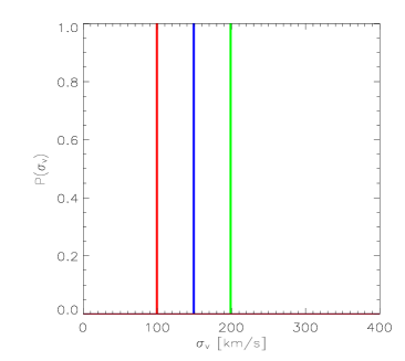
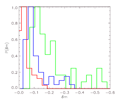
Figure 2: Left panel: velocity dispersions characterizing the MgII absorbing galaxies. Right panel: distributions of quasar magnitude shifts induced by these absorbers, considering the distribution of impact parameters measured by Steidel et al. 

Using the distribution of impact parameters, we can first compute the characteristic magnification expected for a given absorber mass. To do so, we will consider that all absorbing galaxies are identical and we will investigate the effects of isothermal spheres with $\sigma_{v}=100,150$ or $200$ km s^-1. Considering all absorbers to be at redshift $z=0.6$, in order to match the redshifts used by Steidel et al., we can then compute the distribution of induced magnitude shifts $\delta m=-2.5\,\log(\mu)$. The results are shown in Fig. 2. The left panel indicates the different velocity dispersions considered and the right panel shows the corresponding distributions of induced magnitude shifts. As can be seen, if MgII absorbers are typically surrounded by galactic dark matter halos represented by singular isothermal spheres, our calculations show that such a population will change the mean magnitude of their background quasars by $-0.02$ to $-0.2$ typically. Such changes translate into quasar flux increases of about 2 to 20%. However, we recall that these induced magnitude changes are not directly observable. The observed magnitude changes depend on the shape of the luminosity distribution of the sources and will be computed in the section 3.2.

3.1.3 Gas follows dark matter

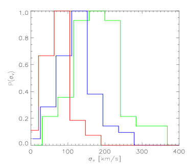
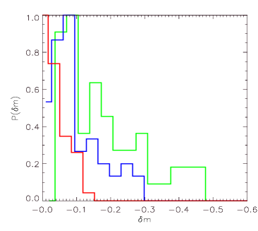
Figure 3: Left panel: distribution of velocity dispersions characterizing the MgII absorbing galaxies obtained by assuming a deterministic relation between gas and mass. Right panel: distributions of quasar magnitude shifts induced by these absorbers, as for Fig. 2

The distribution of absorber rest equivalent widths as a function of impact parameter observed by Steidel et al. (Fig. 1) reveals a correlation at the $3.8\sigma$ level between these two parameters. Such an information can be taken into account in our modelling of the magnification effects. Let us first assume that the gas distribution is proportional to that of the dark matter. In this case we have:

$$\mathrm{N_{MgII}}(b)=\mathrm{f_{MgII}}(b)\times\Sigma(b)$$ (14)

where $\Sigma$ is the total mass surface density, and $\mathrm{f_{MgII}}$ is the MgII to dark matter fraction, i.e. a quantity that depends on the baryon fraction, the metallicity and the ionization background.

It is useful to note that, as infered by Bahcall (1975), the MgII gas distribution within a galactic halo is actually due to a number of individual clouds. This was recently verified by Churchill et al. (1996). Using very high spectroscopic resolution, these authors could detect the absorption lines of individual clouds and they have shown that the overall rest equivalent width $W_{0}$ is proportional to the number of individual velocity components responsible for the global absorption feature. Therefore, assuming that these individual clouds have similar properties we have roughly $W_{0}\propto N_{MgII}$. In this case, the $\mathrm{W_{0}}(b)$ distribution given by Steidel et al. (1994) can then be used to infer a distribution proportional to that of the mass surface densitites:

$$\delta_{\mathrm{D}}\left[\mathrm{W_{0}}(b)\right]\Leftrightarrow\delta_{\mathrm{D}}\left[\Sigma(b)/\Sigma_{0}\right]\Rightarrow\delta_{\mathrm{D}}\left[\sigma_{v}/\sigma_{v,0}\right]\,,$$ (15)

i.e. a given value of rest equivalent width at an impact parameter $b$ maps into a given value of velocity dispersion for which the normalisation $\sigma_{v,0}$ is not known. In this case, the distribution plotted in Fig. 1 provides us with an estimate of the distribution of relative velocity dispersions. For a given normalisation, this distribution can then be used to estimate the expected magnification effects. In order to do so, we convert each data point $\mathrm{W_{0}}(b)$ given by Steidel et al. into as estimate of relative velocity dispersions $\sigma_{v}/\sigma_{v,0}(b)$. We then normalize the distribution of velocity dispersions such that $\langle\sigma_{v}\rangle=100,150$ or $200$ km s^-1. The left panel of Fig. 3 shows the infered distributions of $\sigma_{v}$ and the right panel shows the corresponding distributions of induced magnitude shifts $\mathrm{P}(\delta m)$ for absorbers at redshift $z=0.6$. The changes in the magnitudes of the background quasars are similar to the previous case. They range typically from $-0.02$ to $-0.3$.

3.1.4 Scatter in the gas-dark matter relation

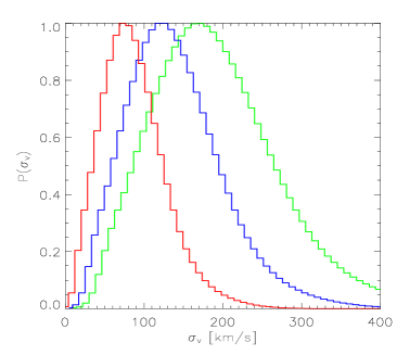
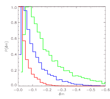
Figure 4: idem as Fig 2 but adding stochasticity in the gas-mass relation using Eq. 16. The width of the distribution $\mathrm{P}(\delta m)$ has increased compared that of Fig 2

In reality, a number of stochastic effects can alter the proportionality between gas and mass distributions, and thus introduce some scatter in the previous relation. For instance, the assumption that all the individual clouds giving rise to the overall absorption feature are similar might not hold, or as it has been argued by Bond et al. (2001), superwinds arising in actively star-forming galaxies can give rise to strong MgII absorption lines seen in some quasar spectra. Therefore it might be more realistic to allow for some scatter in the relation between mass and gas. In order to do so, we can introduce a distribution of velocity dispersions that can give rise to a given gas column density. For example we can use:

$$\delta_{\mathrm{D}}\left[\mathrm{N_{MgII}}\right]\Rightarrow\frac{1}{s\,\sqrt{2\pi}}\;\mathrm{exp}{\left(\frac{-\sigma_{v}^{2}}{2\,s^{2}}\right)}$$ (16)

where $s$ is the scatter in absorber velocity dispersions. Other relations can be used to increase or decrease the scatter of mass with respect to that of the gas. As mentioned previously, observational constraints from higher-order moments will be sensitive to such properties and can allow us to test the validity of a given model. In order to illustrate this idea, we have computed the distribution of induced magnitude changes for the same mean velocity dispersions used in the previous section and we have added a scatter in the absorber velocity dispersion of $\sigma_{v}/4$, where $\sigma_{v}$ is the mean velocity dispersion. A given value $W_{0}$ now maps into a distribution of systems spanning a factor $\sim 3$ in masses. The corresponding magnitude changes are shown in the right panel of Fig. 4. The width of the distribution of induced magnitude changes $\mathrm{P}(\delta m)$ has increased compared to the previous case where an exact proportionality between gas and mass was assumed, and higher magnification values are reached.

3.2 Observable magnitude changes

As shown in section 2, the observable magnitude changes depend on the distribution of induced magnitude shifts $\mathrm{P}(\delta m)$, described in the previous section, as well as the induced quasar magnitude distribution $\mathrm{N_{ref}}(m)$ and the completeness function $\mathrm{C}(m)$ of the relevant survey.
So far, the best estimate of the intrinsic quasar luminosity distribution has been been obtained by Boyle et al. (2000) and Croom et al. (2004) using the 2dF survey. These authors quantified the photometric and spectroscopic imcompleteness of the survey and found that the quasar magnitude distribution is well fitted by a broken power law, as measured by earlier authors. The corresponding fitting formula for the differential number counts reads (Myers et al. 2003):

$$\mathrm{N_{ref}}(m)=\frac{N_{0}}{10^{-\alpha(m-m_{*})}+10^{-\beta(m-m_{*})}}$$ (17)

with $m_{*}=19.1$, $\alpha=0.98$ and $\beta=0.15$. In order to take into account the completeness function, we will consider several forms. First, a completeness corresponding to a purely magnitude limited survey:

$$\mathrm{C_{0}}(m)=\left\{\begin{array}[]{ll}1&\hbox{if $m<m_{limit}$}\\ 0&\hbox{otherwise},\\ \end{array}\right.$$ (18)

where $m_{limit}$ is the limiting magnitude of the survey. For quasars, the color-based selection function introduces a more complicated completeness as a function of magnitude and gives rise to a decrease of $\mathrm{C}(m)$ over some magnitude range. In order to approximate the corresponding behavior we will consider the two following cases:

$$\mathrm{C_{1}}(m)=\left\{\begin{array}[]{ll}1&\hbox{if $m<m_{b}$}\\ \mathrm{e}^{-(m-m_{b})}&\hbox{if $m_{b}<m<m_{limit}$}\\ 0&\hbox{otherwise}\\ \end{array}\right.$$ (19)

$$\mathrm{C_{2}}(m)=\left\{\begin{array}[]{ll}1&\hbox{if $m<m_{b}$}\\ \mathrm{e}^{-(m-m_{b})^{2}}&\hbox{if $m_{b}<m<m_{limit}$}\\ 0&\hbox{otherwise}\\ \end{array}\right.$$ (20)

In order to reproduce realistic observed magnitude distributions for quasars, we will use $m_{limit}=20$ and $m_{b}=17.5$ in our numerical estimates. Note that in this case we have $\mathrm{C}(m)\approx 0$ for $m\approx m_{limit}$. Using $\mathrm{C}_{0}(m)$, $\mathrm{C}_{1}(m)$ and $\mathrm{C}_{2}(m)$ will allow us to estimate how the magnitude changes are sensitive to the shape of the survey completeness.

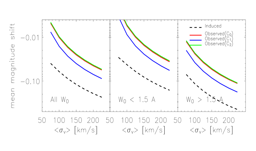
Figure 5: Mean magnitude shifts of quasars due to magnification by intervening MgII absorbers at $z=0.6$, as a function of the mean velocity dispersion of the absorbing galaxies. The dashed curve shows the real mean magnitude shift induced and the colored curves show the mean shift that is observed, as a result of the magnification bias. We have computed the signal expected for the three different completeness functions $\mathrm{C}(m)$ introduced in the text. The left panel shows the effect for absorbers with $0.3<W_{0}<3.3\leavevmode\nobreak\ \mathrm{\AA}$. The middle and right panels show how the signal is expected to vary as a function of rest equivalent width $W_{0}$.

All the elements are now in place to evaluate the observable shifts in the moments of the magnitude distributions, i.e. evaluating Eq. 5 to 8. Fig. 5 shows our computation of the mean magnitude shifts for the fiducial populations of quasars and MgII absorbers, as a function of the mean absorber velocity dispersion. We have plotted here the results obtained using the deterministic relation between gas and mass. However, the values obtained for the other scenarios, i.e. unique absorber mass and stochastic gas-mass relation, are very similar and differ by less than $20\%$. This similarity is due to the fact that the magnification $\mu$ varies roughly linearly with the mass in the weak lensing regime. We have: $\delta m\propto\log(\mu)\propto\mu-1\propto\sigma_{v}^{2}$. Therefore, for the first-order moments, the precise relation between gas and mass does not strongly affect the results, and $\Delta\langle m_{\mathrm{obs}}\rangle$ is primarily a measure of the average mass of absorbers. The left panel of the figure shows the magnitude shifts expected when ones considers the whole range of rest equivalent widths observed by Steidel et al., i.e. $0.3<W_{0}<3.3\leavevmode\nobreak\ \mathrm{\AA}$. The dashed line shows the mean induced magnitude shift $\langle\delta m\rangle$. It ranges from $-0.04$ to $-0.20$ depending of the mean absorber velocity dispersion. The colored lines show the corresponding observable mangnitude shifts $\Delta\langle m_{\mathrm{obs}}\rangle$ for the three completeness functions introduced above. As can be seen, the observable effect is significantly weaker than the real mean magnitude shift induced by the population of absorbers. This is due to the fact that the quasar luminosity distribution departs only weakly from a power law. The observable shift ranges from $-0.005$ to $-0.07$ depending on the completeness function. This signal can be observed as a function of absorber rest equivalent width. In the middle and right panels of Fig 5 we have plotted the same quantities for systems with $W_{0}<1.5\leavevmode\nobreak\ \mathrm{\AA}$ and $W_{0}>1.5\leavevmode\nobreak\ \mathrm{\AA}$. We find that the mean observed magnitude shift $\Delta\langle m_{obs}\rangle$ is roughly three times larger for systems with $W_{0}>1.5\leavevmode\nobreak\ \mathrm{\AA}$ than that of systems with $W_{0}<1.5\leavevmode\nobreak\ \mathrm{\AA}$. Fig 5 provides us with a way of recovering the real magnitude shift $\langle\delta m\rangle$ from the observed one, $\Delta\langle m_{\mathrm{obs}}\rangle$.

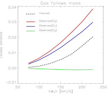
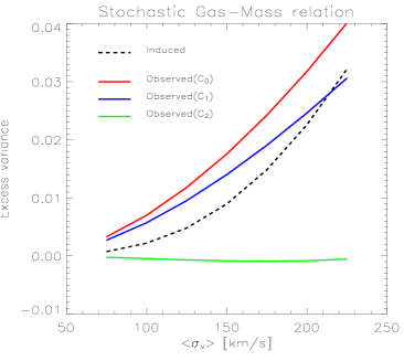
Figure 6: Excess variance of quasars magnitude due to magnification by intervening MgII absorbers. The dashed curve shows the real excess variance induced and the colored curves show the change in the magnitude variance that can be observed. In the left panel we have used a deterministic relation between gas and mass, and in the right panel some stochasticity has been added (see text).

In Fig. 6 we show the results for the second-order moments. The left panel displays the results for the deterministic gas-mass relation. The real excess variance $\langle\delta m^{2}\rangle$ (dashed line) varies from 0.001 to 0.02 depending on the mean absorber velocity dispersion. The colored curves present the corresponding observable magnitude changes $\Delta\langle m_{obs}^{2}\rangle$. Whereas $\langle\delta m^{2}\rangle$ is always a positive quantity, it is interesting to notice that the observable second-order moments changes $\Delta\langle m_{obs}^{2}\rangle$ can be negative in some cases. Indeed, given the existence of a limiting magnitude, shifting the quasar magnitude distribution (Eq. 17) also results in a change of its observed second-order moment. In some cases, depending on the position of the magnitude break $m_{b}$ and the shape of the completeness function, this results in a decrease of the observed magnitude variance. On the other hand, the excess of variance introduced by the existence of a distribution of magnifications tends to increase the observed variance of magnitudes. The net effect can then be either positive or negative. For a given value of $\langle\delta m^{2}\rangle$, $\Delta\langle m_{obs}^{2}\rangle$ is expected to show a strong dependence on the shape of the completeness function $\mathrm{C_{i}}(m)$. The left panel of the figure shows that we expect $\Delta\langle m_{obs}^{2}\rangle$ to lie between $-0.001$ and $0.04$. The right panel of the figure shows the same quantities for the stochastic gas-mass relation, i.e. when a scatter of $\sigma_{v,0}/4$ in the velocity dispersions is added. As expected, the induced magnitude variance is larger than in the previous case. However the changes in the observed second-order moments are rather small compared to the deterministic case: the values of $\Delta\langle m_{obs}^{2}\rangle$ differ only at the $\sim 10^{-3}$ level.

4 Detectability

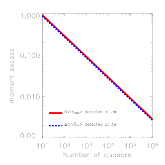
Figure 7: Number of quasars with absorbers required for detecting, at the 3-$\sigma$ level, a change in the magnitude first- (solid line) and second-order (dashed line) moments. For this figure we have considered SDSS quasars observed in the $z$-band.

Whereas our model has provided us with an estimate of the unavoidable magnitude changes $\langle\delta m^{i}\rangle$ due to magnification, it does not allow us to determine, in the general case, the detectability of $\Delta\langle m_{obs}^{i}\rangle$. Including the effects of extinction by dust would be required since they compete against magnification. Unfortunately, the statistical properties of dust extinction of MgII systems are still poorly constrained. The following estimates for the detectability of $\Delta\langle m_{obs}^{i}\rangle$ are therefore valid only if extinction effects can be neglected, as is the case at large wavelengths.

The noise level related to the measurements of the magnitude moments depends on the number of available quasars as well as the shape of the observed magnitude distributions. For a given distribution with centered moments $\langle m^{n}\rangle$ of order $n$ and $N$ objects, the error on the estimation of its mean reads

$$\sigma^{2}(\langle m\rangle)=\frac{\langle m^{2}\rangle}{N}$$ (21)

and the error on the estimation of its variance reads

$$\sigma^{2}(\langle m^{2}\rangle) = \frac{N-1}{N^{3}}\left[(N-1)\langle m^{4}\rangle-(N-3)\langle m^{2}\rangle^{2}\right]$$ (22)

$$\approx \frac{1}{N}(\langle m^{4}\rangle-\langle m^{2}\rangle^{2})$$

In order to estimate these quantities we will use the moments $\langle m^{2}\rangle$ and $\langle m^{4}\rangle$ given by SDSS DR1 quasars (Schneider et al 2003). Using the observed quasar magnitude distribution in $z$-band (where extinction is weaker) we find: $\langle m^{2}\rangle\approx 0.53$ and $\langle m^{4}\rangle\approx 0.75$. Using these values, we show in Fig. 7 the number of quasars required to observe a change in the magnitude first- and second-order moments at the 3$\sigma$ level. Considering that the mean velocity dispersion of MgII absorber systems to be 150 km s^-1, our previous calculations have shown that, $\langle\delta m\rangle\approx-0.15$ and $\langle\delta m^{2}\rangle\approx 0.005$. Using the completeness function $\mathrm{C_{1}}$, the observable changes are $\Delta\langle m_{obs}\rangle\approx-0.1$ and $\Delta\langle m_{obs}^{2}\rangle\approx 0.05$. Figure 7 then shows that $\sim 2000$ systems are required to detect a $3\sigma$ change in the mean magnitude of quasars, and $\sim 10\,000$ for an excess of the magnitude scatter. A detection (or a non-detection) of such mean quasar magnitude shift will provide us with some constraints on the mean mass of the absorbers. This signal can be measured as a function of redshift and rest equivalent width. Our estimate shows that the SDSS survey might already be able to provide us with a detection of the magnitude shift due to gravitational lensing by MgII absorbers. The detection of an excess of variance in the magnitude distributions might be possible. However, the number of quasars required in order to distinguish between a deterministic or stochastic relation between gas and dark matter is several orders of magnitude larger. The corresponding detection level will require next generation surveys.

5 Discussion

Investigating the statistical magnification effects of quasars by intervening absorber systems presents several interests: our calculations have shown that the mean observed magnitude shift $\Delta\langle m_{obs}\rangle$ provides us with an estimate of the mean mass of absorbing galaxies, which turns out to be weakly sensitive to the details of the relation between mass and gas. In addition to probing the mean mass of absorbing galaxies, measuring the mean magnitude shifts $\Delta\langle m_{obs}\rangle$ will also allow us to quantify the real magnitude changes $\langle\delta m\rangle$ that are induced. This will be of direct relevance for estimating the number of quasars missed due extinction by dust or artificially added due to magnification, in magnitude limited surveys. We have shown that quasars behind absorbers are not necessarily dimmed, as is usually mentioned in the literature, but they can actually be brighter if gravitational magnification is more important than extinction effects. By applying our method to MgII lines, we have shown that, if MgII systems trace galactic halos with a mean velocity dispersion $100<\langle\sigma_{v}\rangle<200$ km s^-1, the magnitude of their background quasars will be changed by $-0.03$ to $-0.15$ for systems with $0.3<W_{0}<1.5\leavevmode\nobreak\ \mathrm{\AA}$ and by $-0.1$ to $-0.4$ for systems with $W_{0}>1.5\leavevmode\nobreak\ \mathrm{\AA}$ (see dashed line in Fig 5). In this paper we have considered the absorbing galaxies to be isolated. However, these systems might be correlated to matter overdensities that do not necessarily give rise to absorption lines. For example they might be located in groups of galaxies. In these cases, the lensing effects might be stronger than the ones derived in this paper.
Extinction effects due to high redshift ($z>0.5$) absorbers are currently poorly constrained. As suggested in section 2, their statistical properties can be probed by measuring the quantity $\Delta\langle m_{obs}\rangle_{\lambda}-\Delta\langle m_{obs}\rangle_{\lambda^{\prime}}$ for different wavelengths (Ménard et al., in preparation).

6 Conclusion

We have proposed a method aimed at detecting and interpreting gravitational lensing by absorber systems. Whereas earlier studies focused on strong Lyman-$\alpha$ systems, we suggest to use metal absorbers because they allow for the compilation of larger samples and they can be detected from the ground over favorable redshift ranges for lensing. Due to magnification effects, a given population of absorbers will give rise to a distribution of induced quasar magnitude changes, which is conveniently described by its centered moments $\langle\delta m^{i}\rangle$. The corresponding magnitude changes that can be observed, $\Delta\langle m_{obs}^{i}\rangle=\left\langle{m^{i}_{\mathrm{lens}}}\right\rangle-\left\langle{m^{i}_{\mathrm{ref}}}\right\rangle$, depend on the shape of the quasar luminosity function and the completeness of the survey. We have shown how the observed magnitude changes $\Delta\langle m_{obs}^{i}\rangle$ can be used to recover the induced ones $\langle\delta m^{i}\rangle$ and then constrain the mass distribution of the absorbing galaxies. As a result of the magnification bias, lensing effects can effectively increase or decrease the brightness of the detected sources, depending on their luminosity function. Furthermore if the sources exhibit a power law distribution of luminosities, lensing effects due to absorbers cannot be observed, whatever their amplitude.

Our method can be applied to various absorption lines (MgII, FeII, SiII, CIV, etc.). In order to explore its feasibility, we have computed the expected lensing effects for a population of MgII absorbers. Using the observed distribution of rest equivalent widths as a function of impact parameter measured by Steidel et al.(1994), and assuming that the mass profile of absorber systems is described by that of an isothermal sphere with a mean velocity dispersion $100<\langle\sigma_{v}\rangle<200$ km s^-1, we have shown that:
$\bullet\leavevmode\nobreak\$ Quasars behind MgII absorbers with $0.3<W_{0}<1.5\leavevmode\nobreak\ \mathrm{\AA}$ are in average brighter by $\left\langle\delta m\right\rangle=-0.03$ to $-0.1$ magnitude. For systems with $1.5<W_{0}<3.2\leavevmode\nobreak\ \mathrm{\AA}$ these values reach $-0.1$ to $-0.4$ magnitude.
$\bullet\leavevmode\nobreak\$ The corresponding scatter of magnitude increases by $\left\langle\delta m^{2}\right\rangle=0.01$ to $0.15$ if the gas distribution follows that of the dark matter, and $0.01$ to $0.25$ if we allow for some scatter between these two quantities.
Using the quasar luminosity distribution based on the 2dF Quasar survey (Croom et al. 2004) and realistic completeness functions we have shown that:
$\bullet\leavevmode\nobreak\$ the corresponding magnitude changes that can be observed are $\Delta\langle m_{obs}\rangle=-0.01$ to $-0.04$ for systems with $0.3<W_{0}<1.5\leavevmode\nobreak\ \mathrm{\AA}$, and $-0.03$ to $-0.14$ in the range $1.5<W_{0}<3.2\leavevmode\nobreak\ \mathrm{\AA}$.
$\bullet\leavevmode\nobreak\$ The corresponding variances in observed magnitudes change by $\Delta\langle m_{obs}^{2}\rangle=-0.0005$ to $0.06$. These values turn out to be very sensitive to the shape of the relevant completeness function.

Whereas our model provides us with estimates of the unavoidable magnitude changes $\langle\delta m^{i}\rangle$ due to magnification, it does not allow us to determine, in the general case, the detectability of $\Delta\langle m_{obs}^{i}\rangle$ since effects of extinction by dust need to be included. Observing at sufficiently large wavelengths can however isolate the lensing effects. In this case, we have shown that if MgII absorbers trace galactic halos, about 2000 quasars with such systems will provide us with a detection of the mean magnitude shift due to gravitational lensing. Such a measurement will allow us to constrain the mean mass of absorbing galaxies. Detecting a change in the magnitude distribution variances requires about $10\,000$ quasars with absorbers. However, using our method to probe the stochasticity in the gas-dark matter relation will require next generation surveys.
In this paper we have considered the absorbing galaxies to be isolated. Due to the intrinsic clustering of galaxies, neighoring structures, that do not necessarily give rise to absorption lines, might increase the magnification effects. Quantifying this effect will require further investigations.

In addition to probing the mass distribution of absorber systems, our analysis suggests that quasars behind metal absorbers are not necessarily dimmed, as is usually mentioned in the literature, but they can actually be brighter if extinction effects are smaller than the gravitational magnification effects presented above. The claim that magnitude limited surveys might miss a number of quasars with strong absorbers must therefore be revisited. Applying our method to large surveys will allow us to quantify this effect.

References

- Bahcall (1975) Bahcall, J. N. 1975, ApJ, 200, L1
- Bahcall & Spitzer (1969) Bahcall, J. N. & Spitzer, L. J. 1969, ApJ, 156, L63
- (3) Bartelmann, M. & Loeb, A., 1996, ApJ, 457, 529
- Bartelmann & Schneider (2001) Bartelmann, M. & Schneider, P. 2001, Phys. Rep., 340, 291
- Bergeron & Stasinska (1986) Bergeron, J. & Stasinska, G. 1986, A&A, 169, 1
- Bond, Churchill, Charlton, & Vogt (2001) Bond, N. A., Churchill, C. W., Charlton, J. C., & Vogt, S. S. 2001, ApJ, 562, 641
- Borgeest & Mehlert (1993) Borgeest, U. & Mehlert, D. 1993, A&A, 275, L21
- Boyle et al. (2000) Boyle, B. J., Shanks, T., Croom, S. M., Smith, R. J., Miller, L., Loaring, N., & Heymans, C. 2000, MNRAS, 317,
- Croom et al. (2004) Croom, S. M., Smith, R. J., Boyle, B. J., Shanks, T., Miller, L., Outram, P. J., & Loaring, N. S. 2004, MNRAS, 349, 1397
- Churchill, Steidel, & Vogt (1996) Churchill, C. W., Steidel, C. C., & Vogt, S. S. 1996, ApJ, 471, 164
- Ellison et al. (2004) Ellison, S. L., Ibata, R., Pettini, M., Lewis, G. F., Aracil, B., Petitjean, P., & Srianand, R. 2004, A&A, 414, 79
- (12) Hamana, T., Martel, H., & Futamase, T. 2000, ApJ, 529, 56
- Kobayashi, Terada, Goto, & Tokunaga (2002) Kobayashi, N., Terada, H., Goto, M., & Tokunaga, A. 2002, ApJ, 569, 676
- (14) Le Brun, V., Smette, A., Surdej, J. & Claeskens, J.-F., 2000, A&A 363, 837L
- (15) Maller, A. H., Kolatt, T. S., Bartelmann, M. & Blumenthal, G. R., 2002, ApJ, 569, 72
- Ménard & Péroux (2003) Ménard, B. and Péroux, C., 2003, A&A 410, 43
- (17) Ménard, B., Nestor, D. & Turnshek, D., in preparation
- Myers et al. (2003) Myers, A. D., Outram, P. J., Shanks, T., Boyle, B. J., Croom, S. M., Loaring, N. S., Miller, L., & Smith, R. J. 2003, MNRAS, 342, 467
- (19) Outram, P. J., Smith, R. J., Shanks, T., Boyle, B. J., Croom, S. M., Loaring, N. S. & Miller, L., 2001, MNRAS, 328, 805
- (20) Pei, Y. C., 1995, ApJ, 440, 485
- (21) Perna, R., Loeb, A & Bartelmann, M., 1997, ApJ 448, 550
- Perrotta et al. (2002) Perrotta, F., Baccigalupi, C., Bartelmann, M., De Zotti, G., & Granato, G. L. 2002, MNRAS, 329, 445
- Schneider et al. (2003) Schneider, D. P., et al. 2003, AJ, 126, 2579
- Smette et al. (1995) Smette, A., Robertson, J. G., Shaver, P. A., Reimers, D., Wisotzki, L., & Koehler, T. 1995, A&AS, 113, 199
- (25) Smette, A., Claeskens, J. F. & Surdej, J., 1997, New Astronomy 2, 53
- (26) Steidel, C. C., Dickinson, M. & Persson, S. E., 1994, ApJ, 437, L75
- (27) Steidel, C. C. 1995, astro-ph/9509098
- Thomas & Webster (1990) Thomas, P. A. & Webster, R. L. 1990, ApJ, 349, 437
- Turnshek et al. (1997) Turnshek, D. A., Lupie, O. L., Rao, S. M., Espey, B. R., & Sirola, C. J. 1997, ApJ, 485, 100
- (30) Vanden Berk, D. E., Quashnock, J. M., York, D. G. & Yanny, B., 1996, ApJ 469, 78
- (31) York, D. G., Yanny, B., Crotts, A., Carilli, C., Garrison, E. & Matheson, L., 1991, MNRAS, 250, 24