On the incidence of KHz quasi-periodic oscillations in the neutron star system 4U 1636-53

Abstract

Nearly $1.32\times 10^{6}$ sec of non-zero count rate data were obtained from five years of RXTE observations of the atoll source 4U 1636-53. The data was divided into 10309 segments of 128 sec each. The histogram of the number of segments as a function of count rate shows that the system can naturally be classified into four flux states. For each segment an automated search for kHz QPO was undertaken and the histograms of the maximum Leahy normalised power $P_{max}$ for the four flux states were created. These were fitted by probability distribution functions under the assumption that the intrinsic amplitude of the QPO has a normal distribution. The best fit distribution functions, showed that the fraction $f$ of the time the system exhibits a kHz QPO, decreases from near unity for the lowest flux state ($\approx 1400$ c/s) to zero for the highest one ($>2550$ c/s) while the average amplitude remains nearly constant. Based on the best fit probability distribution functions, a threshold $P_{thre}$ was defined, such that 95% of the segments with $P_{max}>P_{thre}$ correspond to a real QPO signal. For segments selected by this criterion, the frequency versus count rate plot reproduced the earlier known “parallel track” variation with the tracks coinciding roughly with the flux states. It is shown that the gaps between the tracks are not caused by uneven sampling, but rather the QPO phenomenon is absent or weak when the system’s flux level is intermediate between two flux states.

1 Introduction

Rapid (300–1300 Hz), nearly periodic variability in the X-ray light curves of low mass X-ray binary systems (LMXB’s) have been observed by the Rossi X-ray Timing Explorer (RXTE) in over two dozen neutron star bearing LMXB’s (see van der Klis 2000 for a review). These oscillations, referred to as kilohertz QPO (quasi-periodic oscillations), often have high quality factors (Q=FWHM/frequency), and tend to be seen in pairs, with nearly constant frequency separation between the two peaks. The high frequencies of kilohertz QPO strongly suggests that they are related to phenomena taking place in the inner regions of accretion disks surrounding neutron stars, making them potentially valuable probes of strong gravity and the behaviour of matter in such environments.

Several theoretical ideas have been proposed to explain the phenomenology of kilohertz QPO. In these models, one of the frequencies is generally identified as the Keplerian frequency of a characteristic radius of an accretion disk (for e.g. the innermost orbit). In the sonic point model (Miller, Lamb & Psaltis 1998) the second frequency is identified as the beat of the primary QPO with the spin of the neutron star. Stella & Vietri (1999) have proposed a general relativistic precession/apsidal motion model wherein the secondary QPO is due to the relativistic apsidal motion of this characteristic orbit. On the other hand, in the two oscillator model Osherovich & Titarchuk (1999), the secondary frequency is due to the transformation of the primary (Keplerian) frequency in the rotating frame of the neutron star magnetosphere. Recently Lee et al. (2004) have proposed that the QPO occurs at that radius of the disk where local resonance occurs between the Keplerian and epicyclic frequencies. These models are based on their predictions for the variation of the frequency separation with the kilohertz QPO frequency and the variation of the kHz QPO frequency with that of other QPO observed in a source. However a clear consensus regarding which is the viable model has not arisen perhaps because most of these dynamic models generally do not address the direct origin of these oscillations. Using the observed lags in different energy bands, Lee, Misra & Taam (2001), showed that the QPO is driven by a temperature variation in a Comptonizing cloud of size $\approx 10$ km. A unified model for kilohertz QPO, that takes into account both the dynamic and radiative aspects of the phenomenon is still illusive. Such a model should also address how often and under what circumstances does a QPO occur and hence the primary motivation of this work is to quantify the incidence of the kHz QPO phenomenon in the atoll source 4U 1636-53. It is important to know whether the phenomena is a ubiquitous or a transient one, which in turn will provide insight into its cause.

In the next section, we argue that the standard data analysis technique is not adequate to address this question and motivate the need for a modified technique. In that section we highlight the reasons why the atoll source 4U 1636-53 was chosen for the analysis and the need to study the incidence in terms of the long term flux states. In §3 the data analysis technique and the theoretical probability distribution functions which are fitted to the results of the analysis are described. In §4 the results are presented and fitted while in §5 the implications of the results are discussed.

2 Data analysis Technique

The standard technique to analyse the kHz QPO phenomenon is to compute power spectra of segments of the light curve and fit Lorentzian profiles to them. This provides unambiguous measure of the QPO frequency, width and amplitude. Correlation between these quantities and the spectral properties like intensity, hardness ratio can be tested and quantified. However, it is difficult to use this technique to obtain an estimate of the incidence of the QPO phenomenon. To apply this technique, one has to impose a threshold significance level, say $95$% confidence level, that a QPO has been detected for a given segment of data. This means, by definition, that a certain fraction ($5$% in this example) of the segments analysed will have positive but false detections. These detections may be a significant fraction of the real QPO that can be detected in this scheme ( say $10$%). Increasing the threshold level, will decrease the number of QPO detected and biases the result toward high amplitude detections. Another related problem with this analysis technique is the bias in the measure of the amplitude. To illustrate this, consider a long light curve which has a QPO with a constant amplitude $A$, which is less than the threshold significance level of the analysis. The resultant power in each segment due to this QPO will not be a constant but will have statistical fluctuations. Hence, occasionally, the power will be greater than the threshold and this result can be interpreted as being due to a rarer but stronger QPO in the light curve. As noted by Leahy et al. (1983), significance of the presence and amplitude of a detected QPO, should take into account the number of segments and frequency range searched. The results obtained without taking these effects into account maybe biased and should be interpreted with caution.

These deficiencies of the standard data analysis technique are difficult to overcome and hence to make progress, significant trade off in the accuracy and interpretation of the data have to be made. The technique applied in this work, which is described in more detail below, involves finding the Leahy normalised power spectrum for each segment and identifying the maximum power and the frequency at which that occurs. The histogram of the maximum power can then be compared with theoretical probability distributions. The advantage of this method is that there are no thresholds for QPO detections imposed and hence the data is used maximally. However, there are two related drawbacks. First, the peak of the power spectrum is representative of the peak of the Lorentzian fit to the QPO and not the amplitude. To obtain the amplitude one needs to know also the width or Quality factor of the QPO, which is not extracted in this analysis. Second, the theoretical probability distribution, in principle, should also depend on this width or quality factor. Moreover, these probability distributions for Leahy normalised maximum power are computed on the assumption that the the count rate is a constant for different segments, which is not true even when the data is selected for a given intensity state. Taking these effects correctly into account is complicated and hence in this work we make simplistic assumptions when computing the theoretical probability distributions and partially justify our choice by showing that they fit the observed distributions with a reduced $\chi^{2}$ or order unity. This means that more correct but complicated probability distribution functions, perhaps cannot be differentiated by the present data and hence may not be warranted.

The presence and properties of the kHz QPO are expected to be correlated to the source’s spectral parameters (see van der Klis 2000 for a review and references therein). Low mass X-ray binaries containing weakly magnetised neutron stars are divided into two classes based on the Z or atoll like shaped tracks they trace out in colour-colour diagrams. The time-scale to trace out the tracks is typically short ($\mathrel{\mathchoice{\lower 0.5pt\vbox{\halign{$\mathnew\displaystyle\hfil#\hfil$\cr<\crcr\sim\crcr}}}{\lower 0.5pt\vbox{\halign{$\mathnew\textstyle\hfil#\hfil$\cr<\crcr\sim\crcr}}}{\lower 0.5pt\vbox{\halign{$\mathnew\scriptstyle\hfil#\hfil$\cr<\crcr\sim\crcr}}}{\lower 0.5pt\vbox{\halign{$\mathnew\scriptscriptstyle\hfil#\hfil$\cr<\crcr\sim\crcr}}}}$ day), although atoll sources can take longer ($\mathrel{\mathchoice{\lower 0.5pt\vbox{\halign{$\mathnew\displaystyle\hfil#\hfil$\cr<\crcr\sim\crcr}}}{\lower 0.5pt\vbox{\halign{$\mathnew\textstyle\hfil#\hfil$\cr<\crcr\sim\crcr}}}{\lower 0.5pt\vbox{\halign{$\mathnew\scriptstyle\hfil#\hfil$\cr<\crcr\sim\crcr}}}{\lower 0.5pt\vbox{\halign{$\mathnew\scriptscriptstyle\hfil#\hfil$\cr<\crcr\sim\crcr}}}}$ week) to cover the entire curve. The variation in the intensity during such a trace out is typically a factor $\mathrel{\mathchoice{\lower 0.5pt\vbox{\halign{$\mathnew\displaystyle\hfil#\hfil$\cr<\crcr\sim\crcr}}}{\lower 0.5pt\vbox{\halign{$\mathnew\textstyle\hfil#\hfil$\cr<\crcr\sim\crcr}}}{\lower 0.5pt\vbox{\halign{$\mathnew\scriptstyle\hfil#\hfil$\cr<\crcr\sim\crcr}}}{\lower 0.5pt\vbox{\halign{$\mathnew\scriptscriptstyle\hfil#\hfil$\cr<\crcr\sim\crcr}}}}2$, while the changes in the colours (depending on the definition) is typically $\mathrel{\mathchoice{\lower 0.5pt\vbox{\halign{$\mathnew\displaystyle\hfil#\hfil$\cr<\crcr\sim\crcr}}}{\lower 0.5pt\vbox{\halign{$\mathnew\textstyle\hfil#\hfil$\cr<\crcr\sim\crcr}}}{\lower 0.5pt\vbox{\halign{$\mathnew\scriptstyle\hfil#\hfil$\cr<\crcr\sim\crcr}}}{\lower 0.5pt\vbox{\halign{$\mathnew\scriptscriptstyle\hfil#\hfil$\cr<\crcr\sim\crcr}}}}20$%. The kHz QPO properties are known to be correlated to the position of the source in the colour-colour diagram in these timescales. Over longer time-scales the behaviour of the system is more complex. For some of the atoll sources, there are secular variation in the intensity by $\approx 20$% while the response corrected colour-colour track remains nearly invariant (Di Salvo, Mendez & van der Klis 2003). The QPO frequency versus intensity plots show parallel tracks where each track marks the short term correlation between the two (e.g. Mendez et al. 1999 ; Mendez, van der Klis & Ford 2001). This perhaps implies that the properties of the QPO are determined by the spectral shape (i.e. the position in the colour-colour diagram) and not on the long term intensity variations. This is partially supported by the plot of QPO frequency versus position in the colour-colour plot, where the parallel tracks in the intensity plot almost overlap each other (Di Salvo et al., 2003). However, the scatter of the frequencies with respect to colour-colour position is larger than the scatter along each track in the intensity plot. Moreover, for the long term analysis there is no significant correlation between the frequency and colour-colour position (Di Salvo et al., 2003). Evidence that the QPO properties depends on the long term intensity, comes from the frequency-intensity parallel tracks for different sources, where for all of them the low intensity tracks have a wider range of observed frequencies compared to the high intensity tracks. As described in this work, the histogram of the number of detections as a function of intensity shows peaks which nearly coincide with the parallel tracks, which implies that the source has distinguishable intensity (or flux) states. In summary, it is not clear if all of the QPO properties depend only on the spectral shape. The long term intensity may also be an important factor determining some properties especially the incidence.

In this work we quantify the incidence of the QPO phenomenon as a function of different long term intensity states. This source was chosen since a highly coherent kHz ($\approx 800$ Hz) QPO has been observed in its power spectrum Zhang et al. (1996); Wijnands et al. (1997). The second QPO at $\approx 1200$ Hz is weak and in general cannot be detected by the techniques used in this work.

3 Data analysis and Probability distribution functions

Nearly all of the archival RXTE data for the atoll source 4U 1636-52, that had the Event mode data (E_125$\mu$s_64M_0_1s) with $128\mu$sec time resolution, were analysed. The resulting $1.32\times 10^{6}$ sec of non zero count data were divided into $10309$ segments of $128$ sec each. For each segment a power spectrum was obtained at a Nyquist frequency of $4096$ Hz, by averaging $256$ sub-segments of $0.5$ sec each. Thus the power spectra had 2048 frequency bins of width 2 Hz. The power spectrum were Leahy normalised (Leahy et al., 1983) i.e.

$$P(f)=2|a(f)|^{2}/N$$ (1)

where $a(f)$ is the Fast Fourier Transform and $N$ is the total number of counts. For each power spectrum the maximum power $P_{max}$ within the frequency range $200$ to $2000$ Hz and the corresponding frequency $f_{Q}$ were obtained. For each segment we define a normalised count rate $R_{N}\equiv R(5/n_{pon})$ where $R$ is the detected count rate and $n_{pon}$ is the number of proportional counter units (PCU) on during the observation. It should be noted that since in the computation of $R_{N}$, the time dependent detector response is not taken into account, it is at best an approximate representation of the real flux from the source.

In the absence of a signal, the average power at any frequency is $<P>=2$ and the distribution of $P$, $p_{ns}(P)$ is the $\chi^{2}$ distribution with $2M$ degrees of freedom, where $M=256$, is the number of sub-segments Leahy et al. (1983). The probability density of obtaining a $P_{max}$ is

$${\rm P}_{ns}(P_{max},N_{f})=N_{f}\;p_{ns}(P_{max})Q_{ns}(<P_{max})^{N_{f}-1}$$ (2)

where $N_{f}=900$ is the number of frequency bins sampled and

$$Q_{ns}(<P_{max})=\int_{0}^{P_{max}}p_{ns}(P)dP$$ (3)

is the probability that the power in a frequency bin is less than $P_{max}$. In the presence of a signal the computation of the probability density of $P_{max}$, ${\rm P}_{s}(P_{max})$ is more complicated and model dependent. For a pure sinusoidal signal, the average power at the oscillation frequency is Leahy et al. (1983)

$$<P>=2[1+0.19NA^{2}]$$ (4)

where $A$ is the amplitude of the oscillation. It has been assumed here that the oscillation frequency is much smaller than the Nyquist one. The probability distribution $p_{s}(P,N,A)$ can be approximated to be a $\chi^{2}$ distribution of 2M degrees of freedom but rescaled such that the average power is given by eqn (4). The total number of counts $N$ is not a constant even for all segments considered in the same flux state, since the number of PCU that are on during a observation varies. This variation can be taken into account by representing the probability distribution as

$$p_{s}(P,A)=\sum_{i=1}^{5}g_{i}p_{i}(P,N_{i},A)$$ (5)

where $i$ is the number of PCU on, $g(i)$ is the fraction of the time that $i$ PCU were on and $N_{i}$ is the average number of counts when $i$ PCU were on i.e $N_{i}=R_{N}(n_{pon}/5)\times 128$ sec. The above expression assumes that the amplitude of the oscillation is a constant which naturally may not be the case. Moreover, in a defined flux state, the value of $R_{N}$ varies over a range which will affect the predicted average power (eqn 4). Further, the observed QPO is not a pure sinusoidal signal and has a finite width. Taking these effects into account is complicated and hence for simplicity we convolute the probability distribution $p_{s}(P,A)$ with a Gaussian of width $\sigma$ to give a averaged probability distribution $<p_{s}(P,A)>$. The probability density for obtaining $P_{max}$ under these assumption becomes

$${\rm P}_{s}(P_{max},\sigma,A) = {\rm P}_{ns}(P_{max},N_{f}-1)Q_{s}(<P_{max})+$$ (6)

$$<p_{s}(P_{max},A)>Q_{ns}(<P_{max})^{N_{f}-1}$$

where

$$Q_{s}(<P_{max})=\int_{0}^{P_{max}}<p_{s}(P,A)>dP$$ (7)

is the probability that the power in the oscillation frequency bin is less than $P_{max}$. The first term in eqn (6) is the probability density that $P_{max}$ is obtained by chance at any other frequency, while the second term is for the probability of $P_{max}$ to occur at the oscillation frequency. At a given flux state, in general, a signal may exist only for a fraction $f$ of the time. Hence the total probability distribution is

$${\rm P}=f{\rm P}_{s}(P_{max},\sigma,A)+(1-f){\rm P}_{ns}(P_{max},N_{f})$$ (8)

The probability distribution ${\rm P}$ has three unknown parameters $f$, $A$ and $\sigma$ and depends on the known normalised flux $R_{N}$ and PCU on fractions $g_{i}$.

The technique used in this analysis is sensitive only to narrow band, peaked signals. Any broad band component will be spread over all (or a significant fraction of) the 900 frequency bins used. Thus the contribution of a equally strong broad band signal at a given frequency bin would be a large factor ($\approx 100$) less than that of a narrow band signal which is spread over fewer ($\approx 10$) frequency bins. Thus, to effect the analysis a broad band signal would need to have at least $10-100$ time more power than a typical QPO detected ($\approx 5$%). For an average rate of 2000 counts/sec, the Poissonian noise at 500 Hz ( 300 Hz) is 100% (30%) and hence the Poissonian noise is expected to dominate over any underlying broad component which justifies the use of $\chi^{2}$ distribution for $p_{ns}(P)$. However, it should be noted that the effect of any such high frequency broad band noise (e.g. van Straaten et al., 2000) has not been taken into account in this analysis.

4 Results

The histogram of the normalised count rate $R_{N}$ for all the data is shown in Figure 1. $R_{N}$ ranged from $\approx 500$ counts/sec to $\approx 4000$ counts/sec, not including the burst periods. We have classified the data into four flux states which are marked in Figure 1. Data for $R_{N}<1100$ counts/sec have not been shown in the figure, since the low count rate and the relatively small number of detections does not allow for any significant results to be obtained as discussed below. Figure 2 shows the histograms of $P_{max}$ for the four states. The error for each bin was taken to be the square root of the number of detections at that bin. Fitting was done over a continuous range of $P_{max}$ where there were detections. The dotted lines represent the corresponding curves if there were no signals in the data ${\rm P}_{ns}(P_{max})$. Note that there are no free parameters in ${\rm P}_{ns}(P_{max})$ and the good fit to the high state (IV) histogram (reduced $\chi^{2}=0.6$) implies that there are no strong oscillatory signals in this state and the fraction of time a QPO is present during this state is nearly zero. The upper limit on this fraction $f<0.06$ for $A>0.025$ can be inferred. The shape of the histograms for the other three states are clearly different, indicating that there are oscillatory signals at least for some fraction of the time during these states. These histograms were fitted by the probability distribution ${\rm P}$ for different values of fraction $f$, and amplitude $A$ while $\sigma=0.15$ was held constant. The best fit curves (solid lines), the best fit parameter values and the number of degrees of freedom are shown in in Figure 2. Varying $\sigma$ does not change the best fit parameters significantly. For example, for $\sigma=0.25$ the best fit values of $f$ are $0.97$, $0.36$ and $0.15$ for states I,II and III respectively while the corresponding values for $\sigma=0.05$ are $0.8$, $0.30$ and $0.11$. For $R_{N}<1100$ counts/sec, the best fit parameters obtained were $f=1.0^{+0}_{-0.4}$ and $A=.0475\pm 0.005$ which are consistent with the interpretation that $f\approx 1$ for low count rates. The theoretical probability distributions adequately represent the data with reduced $\chi^{2}\approx 1$ for all the fits. Hence more sophisticated probability functions are perhaps not warranted and may lead to over modelling.

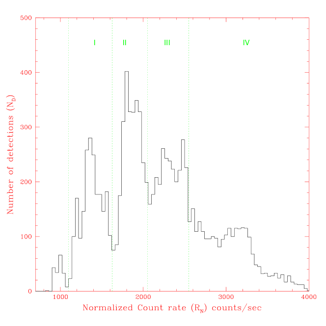
Figure 1: The histogram of normalised count rate $R_{N}$ for all the data sets considered. Four flux states have been identified and marked by roman numerals. I: $1225<R_{N}<1625$ counts/sec, II: $1625<R_{N}<2050$ counts/sec, III: $2050<R_{N}<2550$ counts/sec, IV: $R_{N}>2550$ counts/sec.

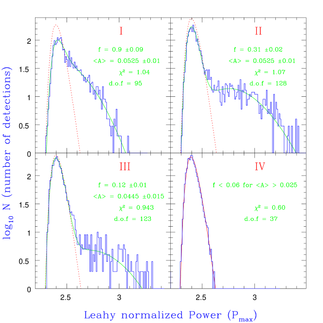
Figure 2: The histograms of the maximum Leahy normalised power $P_{max}$ for four flux states. The dotted line is the expected probability distribution due to statistical fluctuations alone ${\rm P}_{ns}(P_{max})$. The best fit parameters, the reduced $\chi^{2}$ and the number of degrees of freedom, d.o.f, are given. For all probability distributions $\sigma=0.15$.

Based on the best fit probability distribution, We can now define a threshold power $P_{thre}$ such that for 95% of the segments with $P>P_{thre}$, the peak power corresponds to a real signal. The corresponding thresholds for the states, I, II and III turn out to be $2.55$, $2.56$ and $2.60$ respectively. The completeness of this selection criterion i.e. the fraction of the total number of segments with QPO that would be selected turn out to be $0.36$, $0.82$ and $0.69$ for the three states respectively. The corresponding frequencies of the segments with $P>P_{max}$ are shown as a function of the normalised count rate in Figure 3. As expected, the parallel tracks are reproduced. The histogram of the selected segments for different count rates (Figure 4 top panel) shows peaks at the same fluxes as in Figure 1. This may indicate that the gaps in the frequency-flux plot (Figure 3) maybe due to the uneven distribution of fluxes exhibited by this source. However, the ratio of the segments with $P>P_{thre}$ to the total number of segments at a flux level (Figure 4 b) also shows peaks at the same corresponding fluxes. Thus it appears that there are at least three distinct flux levels for this source. The QPO phenomenon appears when the system is in one of these flux level , while in the intermediate flux levels the phenomenon is either weak or absent.

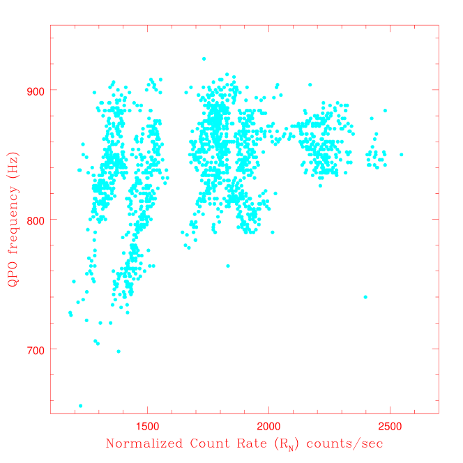
Figure 3: The variation of the QPO frequency for all segments with $P>P_{thre}$ versus the normalised count rate.

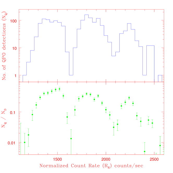
Figure 4: The number of segments with $P>P_{thre}$, $N_{Q}$ (Top panel) and the ratio of $N_{Q}$ to the total number of segments, $N_{D}$ (Bottom panel) as a function of the normalised count rate ($R_{N}$).

The histogram of the number of segments with $P>P_{thre}$ as a function of frequency is shown in figure 5, while figure 6 shows the average peak amplitude $<A_{Q}>$, defined as $A_{Q}\equiv(P-2)/(0.38N)$. Although, $A_{Q}$ is a measure of the peak of the Lorentzian function, rather than the actual amplitude of the QPO, the results obtained here are similar to the result obtained by Mendez et al. (2001); Di Salvo et al. (2003), who found that the amplitude is nearly constant till $f\approx 850$ Hz and then falls off. However, as mentioned earlier these results should be treated with caution since the selection criterion makes the QPO sample incomplete.

For a selection criterion based on flux levels, as has been done in this work, the QPO detected may arise from different parallel tracks. In principle, each track may have a different average amplitude and/or incidence. Such a dichotomy may give rise to a bimodal distribution of QPO powers and should be fitted by two probability distribution functions. This may be particularly true, when the frequency shift between the two tracks is large and the flux range chosen to define a flux level is small. However, the flux range chosen in this work, is sufficiently large such that the corresponding range of frequencies for each track is large with significant overlap. Thus, the distribution of QPO versus frequency (Figure 5) does not show any bimodal structure for states (II) and (III). For state (I) there may be a double peak structure in the distribution. However, for this state the average amplitude does not seem to vary much with frequency (Figure 6) implying perhaps that the average amplitude is nearly same for the two tracks. Fitting the detection distribution versus maximum power (Figure 2; top left panel) with two probability functions, instead of one, does not lead to a reduction in $\chi^{2}$. Instead a degenerate fit where the amplitudes of the two probability distributions are nearly equal and the incidence fractions add up to $\approx 0.9$, is obtained. Any difference between the incidence and average amplitude of the two parallel tracks may be detectable with the use of smaller flux ranges, but this leads poor statistics due to the lower number of detections for each flux level. Alternatively, this may be achieved, by a different selection criteria which uses some other source property that can clearly distinguish and separate out the different parallel tracks. However, it is not clear which source property can be used here, since the QPO frequency has a weak dependence on hardness ratios (Di Salvo et al., 2003).

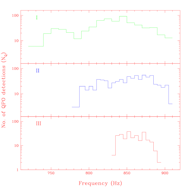
Figure 5: The number of segments with $P>P_{thre}$, $N_{Q}$ versus the QPO frequency for the three lower flux levels (I,II and III).

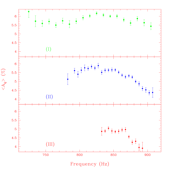
Figure 6: The averaged amplitude $A_{Q}$ for segments with with $P>P_{thre}$, versus the QPO frequency for the three lower flux levels (I,II and III).

5 Summary and Discussion

Based on the histogram of the number of detections as a function of normalised count rate, four distinct flux levels have been defined. It is found that the incidence of kHz QPO, decreases from near unity at low flux levels to nearly zero at high ones. The variation of frequency with count rates reveal roughly three distinct parallel tracks which are coincident with the lower three flux levels. It is however, argued that in the intermediate flux levels, the QPO phenomenon actually disappears or weakens and the parallel tracks are not due to uneven sampling of the source at different intensities.

This analysis suggests that the QPO phenomenon is also related to the long term flux level of the source and in particular occurs more frequently as the flux level decreases. The existence of an inferred threshold accretion rate, beyond which the QPO phenomenon disappears has been suggested earlier (Cui, 2000) based on short term evolution of the source. Here we show that for the long term evolution there exists such a threshold intensity level. Within each long term flux level, it is shown that the QPO weakens and/or disappears as the count rate increases. Thus the phenomenology seems to be more complex than envisioned before. Cui (2000) have proposed that the QPO is produced as a result of the interaction of the magnetosphere with the Keplerian disk, and at high accretion rates, when the magnetosphere radius is smaller than the last stable orbit, the phenomenon disappears. If the magnetosphere radius is the radius at which magnetic pressure equals the ram pressure of freely accreting material, then this model predicts a single accretion rate threshold above which the phenomenon should disappear. Thus this simple model needs to be modified to explain the disappearance or weakening of the QPO phenomenon for each long term flux level. This may not be surprising, because the magnetosphere for this low magnetic field systems, probably depends also on the kind of accretion flow rather than just on the accretion rate and neutron star dipolar field strength.

The presence of parallel tracks in the QPO frequency versus intensity plot, seems to imply that there is more than one parameter that determines the QPO frequency. It is expected that one variable parameter is the accretion rate which should determine the accretion flow and hence QPO properties. It is not clear which is the other varying parameter which gives rise to shifts in the correlation leading to the parallel tracks. van der Klis (2001) showed that this problem can be resolved if the QPO frequency depends on both the prompt and time-averaged value of a single variable parameter. In this scenario, the parallel tracks arise because the time-averaged intensity (or accretion rate) is different for the different tracks. In the simplest version of this model, there is no preferred intensity levels and the distinct tracks are obtained due to observational windowing i.e. the tracks are not connected due to gaps in observations. However, the results obtained in this work suggest that the parallel tracks may correspond to definite flux levels and the gaps in the plot are not due to under sampling. Thus the above model needs to be modified to take into account these observations.

The QPO phenomenon seems to be correlated to long term flux levels on the source in a complex manner, which makes simple theoretical interpretations difficult. The problem is enhanced because as shown in this work the variation of the amplitude of the QPO is affected by the incompleteness arising from the data selection technique. Further, it has been tacitly assumed that in all the flux states, the same QPO is being studied. A clearer idea would arise after a study of the spectral properties of this system. A systematic study of the spectra ( not just the colour which is affected by detector response) of the source at different flux levels and when the QPO is present or not, would shed light into the phenomenon’s origin. It may then be possible, to develop and test theoretical models regarding the nature of these systems.

References

- Cui (2000) Cui W., 2000, ApJ, 534, L31
- Lee et al. (2001) Lee H. C., Misra R., Taam R. E., 2001, ApJ, 549, L229
- Lee et al. (2004) Lee W. H., Abramowicz M. A., Kluzniak W., 2004, ApJ, 603, L93
- Leahy et al. (1983) Leahy D. A. et al. 1983, ApJ, 266. 160
- Mendez et al. (1999) Mendez M., van der Klis M., Ford E. C., Wijnands R., van Paradijs J., 1999, ApJ, 511, L49
- Mendez et al. (2001) Mendez M., van der Klis M., Ford E. C., 2001, ApJ, 561, 1016
- Miller et al. (1998) Miller M.C., Lamb F.K., Psaltis D., 1998, ApJ, 508, 791
- Osherovich & Titarchuk (1999) Osherovich V., Titarchuk L., 1999, ApJ, 522, L113
- Di Salvo et al. (2003) Di Salvo T., Mendez M., van der Klis M., 2003, A & A, 406, 177
- Stella & Vietri (1999) Stella L., Vietri M. 1999, Phys. Rev. Lett., 82, 17
- van Straaten et al. (2000) van Straaten, S., Ford, E. C., van der Klis M., Mendez, M., Kaaret, P. 2000, ApJ, 540, 1049.
- van der Klis (2000) van der Klis M. 2000, ARA&A, 38, 717
- van der Klis (2001) van der Klis M. 2001, ApJ, 561, 943
- Wijnands et al. (1997) Wijnands R. A. D., et al. , 1997, ApJ, 479, L141
- Zhang et al. (1996) Zhang W., Lapidus I., White N. E., Titarchuk L. 1996, ApJ, 473, L135